Exact Nonlinear Model Reduction for a von Kármán beam:
Slow-Fast Decomposition and Spectral Submanifolds

Abstract

We apply two recently formulated mathematical techniques, Slow-Fast Decomposition (SFD) and Spectral Submanifold (SSM) reduction, to a von Kármán beam with geometric nonlinearities and viscoelastic damping. SFD identifies a global slow manifold in the full system which attracts solutions at rates faster than typical rates within the manifold. An SSM, the smoothest nonlinear continuation of a linear modal subspace, is then used to further reduce the beam equations within the slow manifold. This two-stage, mathematically exact procedure results in a drastic reduction of the finite-element beam model to a one-degree-of freedom nonlinear oscillator. We also introduce the technique of spectral quotient analysis, which gives the number of modes relevant for reduction as output rather than input to the reduction process.

1 Introduction

Computer simulations are routinely performed in today’s technological world for modeling and response prediction of almost any physical phenomenon. The ever-increasing demand for realistic simulations leads to a higher level of detail during the modeling phase, which in turn increases the complexity of the models and results in a bigger problem size. Typically, such physical processes are mathematically modeled using partial differential equations (PDEs), which are discretized (e.g. using Finite Elements, Finite differences, Finite volumes methods etc.) to obtain problems with a finite (but usually large) number of unknowns. Despite the tremendous increase in computational power over the past decades, however, the time required to solve high-dimensional discretized models remains a bottleneck towards efficient and optimal design of structures. Model order reduction (MOR) aims to reduce the computational efforts in solving such large problems.

The classical approach to model reduction involves a linear projection of the full system onto a set of basis vectors. This linear projection is characterized by a matrix whose columns span a suitable low-dimensional subspace. Various techniques have been applied to high-dimenisional systems to obain such a reduction basis, including the Proper Orthogonal Decomposition (POD) [9, 10, 11] (also knowns as Singular Value Decomposition (SVD), Karhunen-Loeve Decomposition), Linear Normal Modes (LNM) and Krylov subspace projection [14]. Once a suitable basis is chosen, the reduced-order model (ROM) is then obtained using Galerkin projection. Similar linear projection techniques have been devised for component-mode synthesis (CMS), such as the Craig-Bampton method [13]. An implicit assumption to all linear projection techniques is that the full system dynamics evolves in a lower-dimensional linear invariant subspace of the phase space of the system. While such linear subspaces do exist for linear systems (linear modal subspaces), they are generally non-existent in nonlinear systems. This results in a priori unknown and potentially large errors for linear projection-based reduction methods, necessitating the verification of the accuract of the reduction procedure on a case-by-case basis.

More recent trends in model reduction account for this issue by constructing the reduced solution over nonlinear manifolds [16, 17, 18]. The seminal idea of Shaw and Pierre [24] is to construct assumed nonlinear invariant surfaces (nonlinear normal modes) that act as continuations of linear normal mode families under the addition of nonlinear terms near an equilibrium (see [25] for a recent review). More heuristic reduction procedures in structural dynamics include the static condensation approaches, where the fast or stiff variables in the system are intuitively identified, and statically enslaved to the slow or flexible ones (cf. [19] for a review). Guyan reduction [12] is a classic example of this reduction philosophy at the linear level.

Most classic reduction techniques, coming from a intuive and heuristic standpoint, do not provide an a priori estimate of their accuracy or even validity for a given system. To this effect, Haller and Ponsioen [3] proposed requirements for mathematically justifiable and robust model reduction in a non-linear mechanical system. These requirements ensure not only that the lower dimensional attracting structure (manifold) in the phase space is robust under perturbation, but also that the full system trajectories are attracted to it and synchronize with the reduced model trajectories at rates that are faster than typical rates within the manifold.

Recent advances in nonlinear dynamics enable such an exact model-reduction using the slow-fast decomposition (SFD) [3] and spectral submanifold (SSM) based reduction [4]. SFD is a general procedure to identify if a mechanical system exhibits a global partitioning of degrees of freedom into slow (flexible) and fast (stiff) components such that the fast variables can be enslaved to the slow ones. This results in a global ROM containing only the slow degrees of freedom of the full system. SSMs, on the other hand, are the smoothest nonlinear extensions of the linear modal subspaces near an asymptotically stable equilibrium. Neither SFD nor SSM-based reduction has been applied to problems with high numbers of degrees of freedom. A beam model is often the first step in showing the potential of a new technique for reduction of high dimensional systems (cf. [20, 21, 15]). To this effect, we combine here, for the first time, the application of these techniques on a finite-element discretized nonlinear von Kármán beam model.

We first show that the beam model satisfies the requirements of SFD. The corresponding ROM is subsequently obtained on a slow manifold defined over the transverse degrees of freedom of the beam. This SFD-reduced ROM posseses no clear spectral gaps but a spectral quotient analysis nonetheless enables a further reduction to an SSM using the formulas given by Szalai et. al [6]. Importantly, our spectral quotient analysis returns the number of modes relevant for reduction, instead of postulating or deducing this number from numerical experimentation. In the end, our two-step reduction results in an exact ROM with a drastic reduction in the number of degrees of freedom of the system.

In the next section, we start by reviewing the main steps involved in the derivation of the governing PDEs for the von-Karman beam and the non-dimensionalization we performed upon them. The finite-element disretized equations obtained from the resulting nondimensionalized PDEs are then presented. This system of equations is then first reduced using the SFD in Section 3. The SSM-based reduction applied to the SFD-reduced system in Section 4. The conclusions, along with scope for further work, are presented in Section 5.

Symbol	Meaning (unit)
$L$	Length of beam (m)
$h$	Height of beam (m)
$b$	Width of beam (m)
$A$	Area of cross section (m2) = $bh$
$E$	Young’s Modulus (Pa)
$\kappa$	Viscous damping rate of material (Pa s)
$\rho$	Density (kg/m3)
$\tau$	Non-dimentionalized time

Table 1: Notation

2 Setup

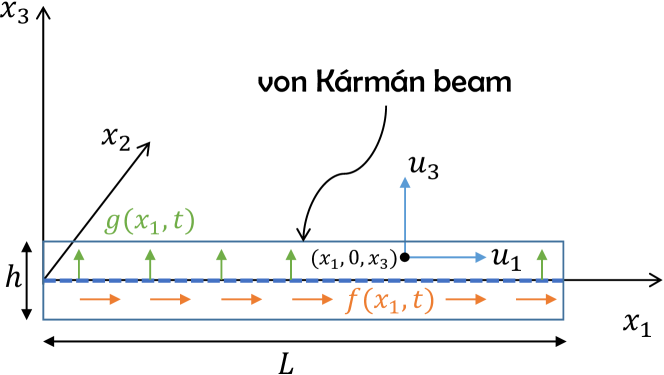
We briefly summarize the main steps leading to the derivation of the governing partial differential equations (PDEs) for the von Kármán beam (see, e.g., Reddy [1] for a detailed derivation). We consider a straight 2D beam aligned initially with the $x_{1}$ axis, as shown in Figure 1. The motion of the beam takes place in the $x_{1}-x_{3}$ plane.

Figure 1: The schematic of a two-dimensional von Kármán beam with height $h$ and length $L$, initially aligned with the $x_{1}$. The $x_{1}$ and $x_{3}$ displacements of a material point with coordinates $(x_{1},0,x_{3})$ are given by $u_{1}$ and $u_{3}$, respectively. The transverse and axial load per unit length applied to the beam are given by $g(x_{1},t)$ and $f(x_{1},t)$, respectively.

Assuming the Euler-Bernoulli hypothesis for the kinematics of bending (i.e., that the lines initially straight and perpendicular to the beam axis remain so after deformation), we obtain the displacement field:

$$u_{1}(x_{1},x_{3}) =u_{0}(x_{1})-x_{3}\partial_{x_{1}}w_{0}(x_{1}),$$

$$u_{2}(x_{1},x_{3}) =0,$$

$$u_{3}(x_{1},x_{3}) =w_{0}\left(x_{1}\right),$$ (1)

where $\left(u_{1},u_{2},u_{3}\right)$ denote the $\left(x_{1},\,x_{2},\,x_{3}\right)$ displacements of a material point with coordinates $(x_{1},0,x_{3})$, and $\left(u_{0}(x_{1}),\,w_{0}(x_{1})\right)$ are the $\left(x_{1},\,x_{3}\right)$ displacements of any material point lying on the reference line given by the $x_{1}$ axis. The von Kármán strain approximation of the Green-Lagrange strain for moderate rotations is given by

$$\varepsilon_{11} =\partial_{x_{1}}u_{0}+\frac{1}{2}(\partial_{x_{1}}w_{0})^{2}-z\partial_{x_{1}}^{2}w_{0}.$$ (2)

Using the virtual work principle, we can formulate the equations of motion in terms of the primary unknowns $u_{0,\,}w_{0}$ as

$$\rho A\mathrm{\partial}_{t}^{2}u_{0}= \,\partial_{x_{1}}\underbrace{\left[\int_{A}\sigma\leavevmode\nobreak\ \mathrm{d}A\right]}_{N}+f(x_{1},t)\,,$$

$$\rho A\mathrm{\partial}_{t}^{2}w_{0}= \,\partial_{x_{1}}^{2}\left[\int_{A}x_{3}\sigma\leavevmode\nobreak\ \mathrm{d}A\right]+\partial_{x_{1}}\left(N\partial_{x_{1}}w_{0}\right)+g(x_{1},t)\,,$$

where $f$ and $g$ are external body forces per unit length of the beam in the $x_{1}$ and $x_{3}$ directions, respectively; $A$ is the area of the cross-section; and $\sigma$ is the $\sigma_{11}$ component of the Cauchy stress. We choose the Kelvin-Voigt model for viscoelasticity as constitutive law to relate the stress $\sigma$ to the von Kármán strain $\varepsilon_{11}$(2) and to the corresponding strain rate as

$$\sigma=E\varepsilon+\kappa\dot{\varepsilon}\,.$$

Here $E$ denotes Young’s modulus and $\kappa$ is the rate of viscous damping for the material. Further assumptions include a uniform rectangular cross section with the reference $x_{1}$ axis passing through the centroid of the cross-section, and a non-dimensionalization of variables as $x=\frac{x_{1}}{L},\,w=\frac{w_{0}}{h},\,u=\frac{u_{0}}{h},\>\tau=\frac{h}{L^{2}}\sqrt{\frac{E}{\rho}}t,\,p(x,\tau)=\frac{\beta L^{4}}{bEh^{4}}f\left(x,\frac{L^{2}}{h}\sqrt{\frac{\rho}{E}}\tau\right),\,q(x,\tau)=\frac{\alpha L^{4}}{bEh^{4}}g\left(x,\frac{L^{2}}{h}\sqrt{\frac{\rho}{E}}\tau\right)$ ($\alpha,\beta$ have been introduced as scaling factors for transverse and axial loading respectively). These lead to the following dimensionless PDEs governing the beam behavior:

$$\ddot{w}+\frac{1}{12}\partial_{x}^{4}w+\frac{\zeta\epsilon}{12}\partial_{x}^{4}\dot{w}-\frac{1}{\epsilon}\partial_{x}\left(\partial_{x}u\,\partial_{x}w\right)-\zeta\partial_{x}(\partial_{x}\dot{u\,}\partial_{x}w)$$

$$-\frac{1}{2}\partial_{x}\left(\partial_{x}w\right)^{3}-\zeta\epsilon\partial_{x}\left(\left(\partial_{x}w\right)^{2}\partial_{x}\dot{w}\right)=\alpha q(x,\tau)\,,$$ (3)

$$\ddot{u}-\frac{1}{\epsilon}\partial_{x}^{2}u-\frac{\zeta}{\epsilon}\partial_{x}^{2}\dot{u}-\frac{1}{2\epsilon}\partial_{x}\left(\partial_{x}w\right)^{2}-\zeta\partial_{x}\left(\partial_{x}w\partial_{x}\dot{w}\right)=\beta p(x,\tau)\,.$$

Here $\dot{(\bullet)}$ denotes $\partial_{\tau}(\bullet)$, $\epsilon=\frac{h}{L}$ is the length to thickness ratio and $\zeta=\frac{\kappa\rho^{1/2}}{E^{3/2}L}$ is a dimensionless constant resulting from non-dimensionalization. We have chosen the displacements to be scaled with respect to the thickness $h$ of the beam, and not the length. Moreover, the applied loading has been nondimensionalized and scaled with respect to a load which leads to transverse displacements in the order of the thickness $h$ of the beam. This is because the von Kármán kinematic approximations are justified for displacements and forces in this range. Furthermore, the time $t$ has been nondimensionalized with respect to a time period that is representatitve of natural frequency of the oscillation of the beam, since the structural response is generally studied at such time scales.

Upon finite-element discretization of the non-dimensional system (3) with cubic shape functions for $w$ and linear shape functions for $u$ (see, e.g., Crisfield [2]), we obtain the finite-dimensional discretized version of (3) as

$$\mathbf{\mathbf{M}}_{1}\ddot{\mathbf{x}}+\zeta\epsilon\left(\mathbf{K}_{1}+\boldsymbol{\mathcal{C}}(\mathbf{x})\right)\dot{\mathbf{x}}+\zeta\boldsymbol{\mathcal{D}}(\mathbf{x})\dot{\mathbf{y}}+\mathbf{K}_{1}\mathbf{x}+\dfrac{1}{\epsilon}\boldsymbol{\mathcal{F}}(\mathbf{x},\mathbf{y})+\boldsymbol{\mathcal{G}}(\mathbf{x})=\mathbf{\alpha q}(\tau)\,,$$

$$\mathbf{\mathbf{M}}_{2}\ddot{\mathbf{y}}+\frac{\zeta}{\epsilon}\mathbf{K}_{2}\dot{\mathbf{y}}+\zeta\boldsymbol{\mathcal{E}}(\mathbf{x})\dot{\mathbf{x}}+\frac{1}{\epsilon^{2}}\mathbf{K}_{2}\mathbf{y}+\dfrac{1}{\epsilon}\boldsymbol{\mathcal{H}}(\mathbf{x})=\beta\mathbf{p}(\tau),$$ (4)

where $\mathbf{x}\in\mathbb{R}^{n_{s}},\mathbf{y}\in\mathbb{R}^{n_{f}}$ are the finite dimensional (discretized) counterparts of the unknowns $w,u$ respectively ($n_{s},\,n_{f}$ being the number of unknowns dependent on the finite-element discretization), and $\mathbf{\mathbf{M}}_{1},\mathbf{\mathbf{K}}_{1}\in\mathbb{R}^{n_{s}\times n_{s}}$ and $\mathbf{\mathbf{M}}_{2},\mathbf{\mathbf{K}}_{2}\in\mathbb{R}^{n_{f}\times n_{f}}$ are the corresponding mass and stiffness matrices. Here, $\boldsymbol{\mathcal{F}}$ (a bilinear function of the form $\left(\boldsymbol{\mathcal{F}}(\mathbf{x},\mathbf{y})\right)_{i}=F_{ijk}x_{j}y_{k},\,i,j\in\{1,\dots,n_{s}\},\,k\in\{1,\dots,n_{f}\}$), $\boldsymbol{\mathcal{G}}$ (a cubic function of the form $\left(\boldsymbol{\mathcal{G}}(\mathbf{x})\right)_{i}=G_{ijkl}x_{j}x_{k}x_{l},\,i,j,k,l\in\{1,\dots,n_{s}\}$) and $\boldsymbol{\mathcal{H}}$ (a quadratic function of the form $\left(\boldsymbol{\mathcal{H}}(\mathbf{x})\right)_{i}=H_{ijk}x_{j}x_{k},\,i\in\{1,\dots,n_{f}\},\,j,k\in\{1,\dots,n_{s}\}$) correspond to the nonlinear elastic forces in the beam; $\boldsymbol{\mathcal{C}}$ (a quadratic function of the form $\left(\boldsymbol{\mathcal{C}}(\mathbf{x})\right)_{ij}=C_{ijkl}x_{k}x_{l},\,i,j,k,l\in\{1,\dots,n_{s}\}$), $\boldsymbol{\mathcal{D}}$ (a linear function of the form $\left(\boldsymbol{\mathcal{D}}(\mathbf{x})\right)_{ij}=D_{ijk}x_{k},\,i,k\in\{1,\dots,n_{s}\},\,j\in\{1,\dots,n_{f}\}$) and $\boldsymbol{\mathcal{E}}$ (a linear function of the form $\left(\boldsymbol{\mathcal{E}}(\mathbf{x})\right)_{ij}=E_{ijk}x_{k},\,j,k\in\{1,\dots,n_{s}\},\,i\in\{1,\dots,n_{f}\}$) correspond to the nonlinear contributions resulting from the viscoelastic material damping.

3 Slow-Fast Decomposition

3.1 Verification of assumptions for the application of SFD

In the finite-element discretized system (4), the $\mathbf{y}$ variables (representing the axial displacement components) are stiffer and hence faster than the $\mathbf{x}$ variables (representing the transverse displacement components). Such a global difference of speeds indicates the possible existence of a lower-dimensional slow manifold, as described in mathematical terms by the geometric singular perturbation theory of Fenichel [5]. If such a slow manifold is robust and attracts nearby solutions, then the dynamics on this manifold provides and exact reduced-order model with which all nearby solutions synchronize exponentially fast.

For general finite-dimensional mechanical systems characterized by such a dicotomy of time scales, Haller and Ponsioen [3] deduced conditions under which positions and velocities in the fast degrees of freedom ($\mathbf{y}$,$\dot{\mathbf{y}}$) can be expressed as a graph over their slow counterparts ($\mathbf{x}$,$\dot{\mathbf{x}}$), resulting in a globally exact model reduction. If these conditions for a Slow-Fast Decomposition (SFD) are satisfied, then all trajectories of the full system (close enough to the slow manifold in the phase space) synchronize with the reduced model trajectories at rates faster than those within the slow manifold. To check these conditions, we take $0<\epsilon\ll 1$, the thickness to length ratio of the beam, as the required non-dimensional small parameter. The system (4) can then be reformulated in terms of $\frac{\mathbf{y}}{\epsilon}$ as

$$\mathbf{\mathbf{M}}_{1}\ddot{\mathbf{x}}+\zeta\epsilon\left(\mathbf{K}_{1}+\boldsymbol{\mathcal{C}}(\mathbf{x})\right)\dot{\mathbf{x}}+\zeta\boldsymbol{\mathcal{D}}(\mathbf{x})\dot{\mathbf{y}}+\mathbf{K}_{1}\mathbf{x}+\boldsymbol{\mathcal{F}}\left(\mathbf{x},\frac{\mathbf{y}}{\epsilon}\right)+\boldsymbol{\mathcal{G}}(\mathbf{x})=\mathbf{\alpha q}(\tau)\,,$$

$$\mathbf{\mathbf{M}}_{2}\ddot{\mathbf{y}}+\frac{\zeta}{\epsilon}\mathbf{K}_{2}\dot{\mathbf{y}}+\zeta\boldsymbol{\mathcal{E}}(\mathbf{x})\dot{\mathbf{x}}+\frac{1}{\epsilon}\mathbf{K}_{2}\frac{\mathbf{y}}{\epsilon}+\dfrac{1}{\epsilon}\boldsymbol{\mathcal{H}}(\mathbf{x})=\mathbf{\beta p}(\tau).$$ (5)

The mass-normalized forcing terms are defined in terms of the new variable $\boldsymbol{\eta}=\frac{\mathbf{y}}{\epsilon}$ as

$$\mathbf{P}_{1}(\mathbf{x},\dot{\mathbf{x}},\boldsymbol{\eta},\dot{\mathbf{y}},\tau;\epsilon) =-\mathbf{\mathbf{M}}_{1}^{-1}\left(\zeta\epsilon\left(\mathbf{K}_{1}+\boldsymbol{\mathcal{C}}(\mathbf{x})\right)\dot{\mathbf{x}}+\zeta\boldsymbol{\mathcal{D}}(\mathbf{x})\dot{\mathbf{y}}+\mathbf{K}_{1}\mathbf{x}+\mathcal{\boldsymbol{F}}\left(\mathbf{x},\boldsymbol{\eta}\right)+\boldsymbol{\mathcal{G}}(\mathbf{x})-\mathbf{\alpha q}(\tau)\right)\,,$$

$$\mathbf{P}_{2}(\mathbf{x},\dot{\mathbf{x}},\boldsymbol{\eta},\dot{\mathbf{y}},\tau;\epsilon) =-\epsilon\mathbf{\mathbf{M}}_{2}^{-1}\left(\frac{\zeta}{\epsilon}\mathbf{K}_{2}\dot{\mathbf{y}}+\zeta\boldsymbol{\mathcal{E}}(\mathbf{x})\dot{\mathbf{x}}+\frac{1}{\epsilon}\mathbf{K}_{2}\boldsymbol{\eta}+\dfrac{1}{\epsilon}\boldsymbol{\mathcal{H}}(\mathbf{x})-\mathbf{\beta p}(\tau)\right)$$ (6)

$$=-\mathbf{M}_{2}^{-1}\left(\zeta\mathbf{K}_{2}\dot{\mathbf{y}}+\epsilon\zeta\boldsymbol{\mathcal{E}}(\mathbf{x})\dot{\mathbf{x}}+\mathbf{K}_{2}\boldsymbol{\eta}+\boldsymbol{\mathcal{H}}(\mathbf{x})-\epsilon\mathbf{\beta p}(\tau)\right).$$

The main conditions of the SFD procedure, as derived by Haller and Ponsioen [3], are the following.

(A1)

Nonsingular extension to $\epsilon=0$: $\mathbf{P}_{1}$ and $\mathbf{P}_{2}$ should possess smooth (in fact $C^{\infty}$) extension to their respective $\epsilon=0$ limits, which is the case here by (6).

(A2)

Existence of a critical manifold: The algebraic equation $\mathbf{P}_{2}(\mathbf{x},\dot{\mathbf{x}},\boldsymbol{\eta},\mathbf{0},\tau;0)\equiv\mathbf{0}$ should be solvable for $\boldsymbol{\eta}$ on an open, bounded domain. Indeed, for any $\mathcal{D}_{0}\subset\mathbb{R}^{n_{s}}\times\mathbb{R}^{n_{s}}\times\mathcal{T}$ open and bounded, the set $\mathcal{M}_{0}(\tau)$ defined by

$$\boldsymbol{\eta}=\mathbf{G}_{0}(\mathbf{x},\dot{\mathbf{x}},\tau):=-\mathbf{K}_{2}^{-1}\boldsymbol{\mathcal{H}}(\mathbf{x})$$

satisfies $\mathbf{P}_{2}(\mathbf{x},\dot{\mathbf{x}},\mathbf{G}_{0}(\mathbf{x},\dot{\mathbf{x}},\tau),\mathbf{0},\tau;0)\equiv\mathbf{0}$ for all $(\mathbf{x},\dot{\mathbf{x}},\tau)\in\mathcal{D}_{0}$, forming a critical manifold $\mathcal{M}_{0}$ in the language of singular perturbation theory. Clearly, the critical manifold is independent of $\tau$ in our current setting. If, however, we assumed that$\beta=\mathcal{O}(\frac{1}{\epsilon})$ (i.e., the beam is excited in the axial direction by forces that are an order of magnitude larger than those in the transverse direction), then we would obtain a time-dependent critical manifold.

Notation:

For clarity, we denote any expression $(\bullet)$ evaluated over the critical manifold $\mathcal{M}_{0}$ by $\overline{(\bullet)}:=(\bullet)|_{\boldsymbol{\eta}=\mathbf{G}_{0}(\mathbf{x},\dot{\mathbf{x}},\tau),\,\dot{\mathbf{y}}=\mathbf{0},\,\epsilon=0}$

(A3)

Asymptotic stability of the critical manifold: With the matrices

$$\mathbf{A}(\mathbf{x},\dot{\mathbf{x}},\tau) =-\partial_{\dot{\mathbf{y}}}\mathbf{P}_{2}(\mathbf{x},\dot{\mathbf{x}},\mathbf{G}_{0}(\mathbf{x},\dot{\mathbf{x}},\tau),\mathbf{0},\tau;0)=-\overline{\partial_{\dot{\mathbf{y}}}\mathbf{P}_{2}}=\zeta\mathbf{M}_{2}^{-1}\mathbf{K}_{2},$$

$$\mathbf{B}(\mathbf{x},\dot{\mathbf{x}},\tau) =-\partial_{\boldsymbol{\eta}}\mathbf{P}_{2}(\mathbf{x},\dot{\mathbf{x}},\mathbf{G}_{0}(\mathbf{x},\dot{\mathbf{x}},\tau),\mathbf{0},\tau;0)=-\overline{\partial_{\boldsymbol{\eta}}\mathbf{P}_{2}}=\mathbf{M}_{2}^{-1}\mathbf{K}_{2},$$ (7)

the equilibrium solution $\boldsymbol{\eta}\equiv\mathbf{0}\in\mathbb{R}^{n_{f}}$ of the unforced, constant-coefficient linear system

$$\boldsymbol{\eta}{}^{\prime\prime}+\mathbf{A}(\mathbf{x},\dot{\mathbf{x}},\tau)\boldsymbol{\eta}^{\prime}+\mathbf{B}(\mathbf{x},\dot{\mathbf{x}},\tau)\boldsymbol{\eta}\Leftrightarrow\mathbf{M}_{2}\boldsymbol{\eta}{}^{\prime\prime}+\zeta\mathbf{K}_{2}\boldsymbol{\eta}^{\prime}+\mathbf{K}_{2}\boldsymbol{\eta} =\mathbf{0}=\mathbf{0}$$ (8)

should be asymptotically stable for all fixed parameter values $(\mathbf{x},\dot{\mathbf{x}},\tau)\in\mathcal{D}_{0}$. This is again satisfied in our setting since $\mathbf{M}_{2},\mathbf{K}_{2}$ are positive definite matrices and $\zeta>0$.

3.2 Global reduced-order model from SFD

As shown by Haller and Ponsioen [3], assumptions (A1)-(A3) guarantee that the critical manifold $\mathcal{M}_{0}(\tau)$ perturbs into a nearby attracting slow manifold $\mathcal{M}_{\epsilon}(\tau)$ for $\epsilon>0$ small enough. On this slow manifold, the discretized beam system (4) admits an exact reduced order model given by

$$\ddot{\mathbf{x}}-\overline{\mathbf{P}_{1}}-\epsilon\left[\overline{\partial_{\boldsymbol{\eta}}\mathbf{P}_{1}}\mathbf{G}_{1}(\mathbf{x},\dot{\mathbf{x}},\tau)+\overline{\partial_{\dot{\mathbf{y}}}\mathbf{P}_{1}}\mathbf{H_{0}}(\mathbf{x},\dot{\mathbf{x}},\tau)+\overline{\partial_{\epsilon}\mathbf{P}_{1}}\right]+\mathcal{O}(\epsilon^{2})=\mathbf{0},$$ (9)

where

$$\mathbf{H}_{0}(\mathbf{x},\dot{\mathbf{x}},\tau) =\left[\partial_{\mathbf{x}}\mathbf{G}_{0}(\mathbf{x},\dot{\mathbf{x}},\tau)\right]\dot{\mathbf{x}}+\left[\partial_{\dot{\mathbf{x}}}\mathbf{G}_{0}(\mathbf{x},\dot{\mathbf{x}},\tau)\right]\overline{\mathbf{P}_{1}}+\partial_{\tau}\mathbf{G}_{0}(\mathbf{x},\dot{\mathbf{x}},\tau)\,,$$

$$\mathbf{G}_{1}(\mathbf{x},\dot{\mathbf{x}},\tau) =\left[\overline{D_{\boldsymbol{\eta}}\mathbf{P}_{2}}\right]^{-1}\overline{D_{\dot{\mathbf{y}}}\mathbf{P}_{2}}\mathbf{H}_{0}(\mathbf{x},\dot{\mathbf{x}},\tau)$$

constitute the higher-order terms in the equations describing the slow manifold $\mathcal{M}_{\epsilon}(\tau)$ as

$$\mathbf{y} =\epsilon\mathbf{G}_{0}(\mathbf{x},\dot{\mathbf{x}},\tau)+\epsilon^{2}\mathbf{G}_{1}(\mathbf{x},\dot{\mathbf{x}},\tau)+\mathcal{O}\left(\epsilon^{3}\right)\,,$$

$$\dot{\mathbf{y}} =\epsilon\mathbf{H}_{0}(\mathbf{x},\dot{\mathbf{x}},\tau)+\mathcal{O}\left(\epsilon^{2}\right)\,.$$ (10)

In the context of the beam example considered here, the exact reduced-order model in (9) can be explicitly written out in the following form:

$$\mathbf{M}_{1}\ddot{\mathbf{x}}+\mathbf{K}_{1}\mathbf{x}+\boldsymbol{\mathcal{F}}\left(\mathbf{x},\mathbf{G}_{0}(\mathbf{x},\dot{\mathbf{x}},\tau)\right)+\boldsymbol{\mathcal{G}}(\mathbf{x})+$$

$$\epsilon\left[\underbrace{\overline{\partial_{\boldsymbol{\eta}}\boldsymbol{\mathcal{F}}\left(\mathbf{x},\boldsymbol{\eta}\right)}\mathbf{G}_{1}(\mathbf{x},\dot{\mathbf{x}},\tau)}_{\mathrm{conservative\,correction}}+\underbrace{\zeta\left(\boldsymbol{\mathcal{D}}(\mathbf{x})\mathbf{H}_{0}(\mathbf{x},\dot{\mathbf{x}},\tau)+\left(\mathbf{K}_{1}+\boldsymbol{\mathcal{C}}(\mathbf{x})\right)\dot{\mathbf{x}}\right)}_{\mathrm{damping\,terms}}\right]+\mathcal{O}\left(\epsilon^{2}\right)=\alpha\mathbf{q}(\tau),$$ (11)

where

$$\mathbf{G}_{0}(\mathbf{x},\dot{\mathbf{x}},\tau) =-\mathbf{K}_{2}^{-1}\boldsymbol{\mathcal{H}}(\mathbf{x})\,,$$

$$\mathbf{H}_{0}(\mathbf{x},\dot{\mathbf{x}},\tau) =-\mathbf{K}_{2}^{-1}\left[\partial_{\mathbf{x}}\boldsymbol{\mathcal{H}}(\mathbf{x})\right]\dot{\mathbf{x}}\,,$$

$$\mathbf{G}_{1}(\mathbf{x},\dot{\mathbf{x}},\tau) =-\zeta\left(\mathbf{H}_{0}(\mathbf{x},\dot{\mathbf{x}},\tau)+\mathbf{K}_{2}^{-1}\boldsymbol{\mathcal{E}}(\mathbf{x})\dot{\mathbf{x}}\right)+\mathbf{\beta K}_{2}^{-1}\mathbf{p}(\tau)\,.$$ (12)

Note that the reduced order model (11) is conservative (contains only inertial and elastic force terms) at leading order, whereas the full system (4) is dissipative due to viscoelastic damping. The $\mathcal{O}(\epsilon)$ terms in the ROM account for these damping contributions and hence cannot be ignored. Apart from the damping contributions, there also exists a conservative correction at the $\mathcal{O}(\epsilon)$ level which includes the static response of the $\mathbf{y}$ variables to the corresponding loading $\beta\mathbf{p}(\tau)$ (cf. the expression for $\mathbf{G}_{1}(\mathbf{x},\dot{\mathbf{x}},\tau)$ in (12)).

3.3 Specific results from SFD

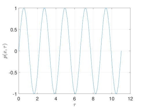
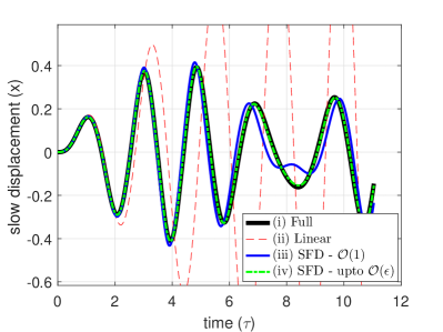
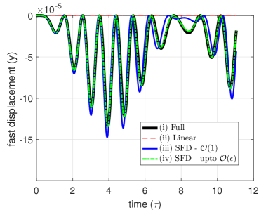
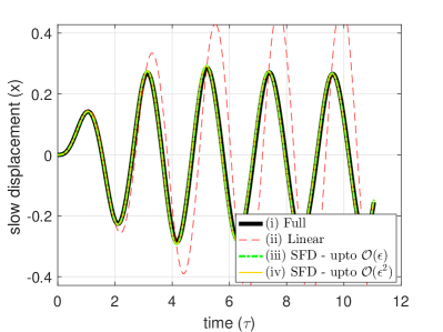
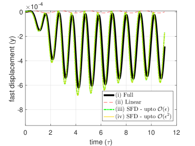
We now consider a specific beam with geometric and material parameters as follows: length $L=1$ m; thickness to length ratio $\epsilon$ in the range from $10^{-4}-10^{-2}$; Young’s modulus $E=70$ GPa; density$\rho=2700$ Kg/m³; material viscous damping rate$\kappa=10^{8}$ Pa s. We use a spatially uniform load on the beam in the axial and in the transverse direction, given by $\alpha=1$ , $\beta=1$, $q(x,\tau)=p(x,\tau)=\sin\left(\Omega T_{0}\tau\right)$. Here $T_{0}=\frac{L}{\epsilon}\sqrt{\frac{\rho}{E}}$ is the constant used to nondimensionalize time and $\Omega$ is the loading frequency (chosen to be the first natural frequency of the beam in this case, cf. Figure 3). Using these parameters, we obtain $\zeta\approx 7.2739$.

Figure 2: The applied loading

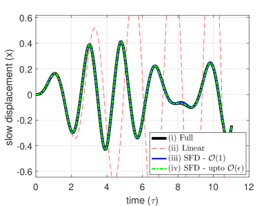
(a) Displacement [-] of the beam at quarter length in the transverse direction (slow $\mathbf{x}$ DOF).

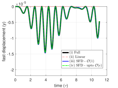
(b) Displacement [-] of the beam at quarter length in the axial direction (fast $\mathbf{y}$ DOF).

Figure 3: Comparison of the slow and fast components of the reduced solution with their full nonlinear and linearized counterparts for $\epsilon=10^{-4}$. Note that for such small values of $\epsilon$, the ROM at the leading order (containing only conservative terms) is a good enough representation of the full system, and is practically identical to ROMs obtained by inclusion of the $\mathcal{O}(\epsilon)$ and $\mathcal{O}\left(\epsilon^{2}\right)$ terms.

(a) Displacement [-] of the beam at quarter length in the transverse direction (slow $\mathbf{x}$ DOF).

(b) Displacement [-] of the beam at quarter length in the axial direction (fast $\mathbf{y}$ DOF).

Figure 4: Comparison of the slow and fast components of the reduced solution with their full nonlinear and linearized counterparts for $\epsilon=10^{-3}$ . For this larger value of $\epsilon$, the leading-order conservative ROM is not accurate enough, and hence $\mathcal{O}(\epsilon)$ terms (which include damping contributions) are required to improve accuracy.

(a) Displacement [-] of the beam at quarter length in the transverse direction (slow $\mathbf{x}$ DOF).

(b) Displacement [-] of the beam at quarter length of beam in the axial direction (fast $\mathbf{y}$ DOF).

Figure 5: Comparison of the slow and fast components of the reduced solution with their full nonlinear and linearized counterparts for $\epsilon=10^{-2}$. The $\mathcal{O}\left(\epsilon^{2}\right)$ terms were added in the ROM to improve accuracy (especially in the slave variables), but only a marginal improvement was observed.

The graphs presented above show the response of a single degree of freedom in time. In order to check the performance of SFD globally, we use the following measure,

$$E=\dfrac{\sqrt{\sum\limits_{\tau\in S}(\mathbf{u}(\tau)-\tilde{\mathbf{u}}(\tau))^{T}(\mathbf{u}(\tau)-\tilde{\mathbf{u}}(\tau))}}{\sqrt{\sum\limits_{\tau\in S}\mathbf{u}(\tau)^{T}\mathbf{u}(\tau)}}\times 100\%\,,$$ (13)

where $\mathbf{u}(\tau)\in\mathbb{R}^{n_{s}+n_{f}}$ is the full vector of generalized displacements at time $\tau$, obtained from the full nonlinear solution; $\tilde{\mathbf{u}}(\tau)\in\mathbb{R}^{n_{s}+n_{f}}$ is the solution based on the reduced model; and $S$ is the set of time instants at which the error is recorded. The error recorded for different cases is shown in Table 2. We observe that for $\epsilon$ of order $10^{-4}$, the ROM at the leading order (which is conservative) provides a close approximation for the full system. The $\mathcal{O}(\epsilon)$ terms, however, become important when $\epsilon$ is of order $10^{-3}$, because they account for damping which becomes more significant in this$\epsilon$-range. We further calculated the $\mathcal{O}\left(\epsilon^{2}\right)$ terms in the ROM to compare changes in accuracy (see A for general calculation of the $\mathcal{O}\left(\epsilon^{2}\right)$ terms). We observe that the $\mathcal{O}\left(\epsilon^{2}\right)$ terms only provide a marginal improvement in terms of accuracy in our case. A further increase in $\epsilon$ values to the order of $10^{-1}$ renders the reduced model highly inaccurate, thus higher-order terms in $\epsilon$ are necessary to achieve the desired accuracy. Note, however, the $\epsilon$ values around $10^{-1}$ are rather unphysical; the parameter $\epsilon$, denoting the thickness-to-length ratio of a beam, is not expected attain such high values.

$\epsilon$	SFD - $\mathcal{O}(1)$	SFD - up to $\mathcal{O}(\epsilon)$	SFD - up to $\mathcal{O}\left(\epsilon^{2}\right)$
$10^{-4}$	3.7078	0.3670	0.3670
$10^{-3}$	29.589	2.9681	2.9681
$10^{-2}$	>100	5.3432	5.3425
$10^{-1}$	>100	>100	>100

Table 2: Relative reduction error $E$ calculated according from formula (13)

4 SSM reduction

Though the SFD reduction is robust and globally valid in the phase space, the reduced system on the slow manifold still contains $n_{s}$ degrees of freedom, which is generally a large number. Specifically, due to the choice of the shape functions for discretization, the reduced model (11) obtained from SFD still contains two-thirds of the total number of unknowns of the full system (4). The following eigenvalue analysis of the linearized reduced system, however, reveals the existence of a further separation in time scales within the slow manifold near the origin, showing potential for a further reduction via spectral submanifolds (cf. Haller and Ponsioen [4])

4.1 Separation in damping: spectral quotient analysis

The eigenvalue problem for the linearization of the reduced system (11) can be formulated as

$$(\lambda_{k}^{2}\mathbf{M}_{1}+\lambda_{k}\zeta\epsilon\mathbf{K}_{1}+\mathbf{K}_{1})\boldsymbol{\phi}_{k}=\mathbf{0}\,,$$ (14)

where $\lambda_{k}\in\mathbb{C}$ and $\boldsymbol{\phi}_{k}\in\mathbb{C}^{n_{s}}$ are the $k^{\mathrm{th}}$ eigenvalue and eigenvector for any $k\in\{1,\dots,n_{s}\}$. The negative real part of the eigenvalue $\lambda_{k}$ represents the exponential rate of decay of trajectories towards the equilibrium position along the corresponding two-dimensional eigenspace of the linearized system. The smoothest local extension of such an invariant subspace is known as the spectral submanifold (SSM), a notion introduced by Haller and Ponsioen [4]. Tangent to a slow subspace (i.e. , the subspace spanned by eigenvectors corresponding to eigenvalues with the lowest-magnitude real parts), such an SSM offers an opportunity for a further, drastic reduction from the SFD-based slow manifold to a two-dimensional invariant manifold.

Estimating the real parts of the eigenvalues arising from (14) is sensitive to the choice of the eigensolver algorithm, especially for large $n_{s}$ values. An accurate first-order approximation to the eigenvalues, however, can be obtained using the undamped eigenvalues from their defining equation

$$(\mathbf{K}_{1}-\omega_{0k}^{2}\mathbf{M}_{1})\boldsymbol{\phi}_{0k}=\mathbf{0}\,.$$

Specifically, for small damping and well-separated eigenvalues, a reliable first-order approximation for the real parts of the eigenvalues of system (14) can be obtained as follows [7]:

$$\lambda_{k}=-\frac{\boldsymbol{\phi}_{0k}^{T}(\zeta\epsilon\mathbf{K}_{1})\boldsymbol{\phi}_{0k}}{2\boldsymbol{\phi}_{0k}^{T}\mathbf{M}_{1}\boldsymbol{\phi}_{0k}}+i\,\omega_{0k}^{2}+\mathcal{O}\left(\epsilon^{2}\right)=-\frac{\zeta\epsilon}{2}\omega_{0k}^{2}+i\,\omega_{0k}^{2}+\mathcal{O}\left(\epsilon^{2}\right)\quad\forall k\in\{1,\dots,n_{s}\}\,.$$ (15)

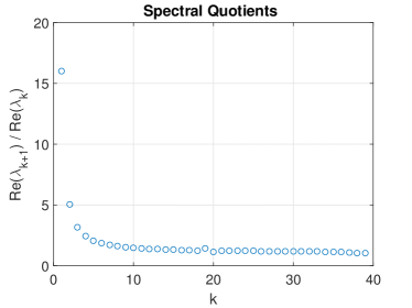
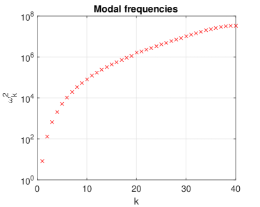
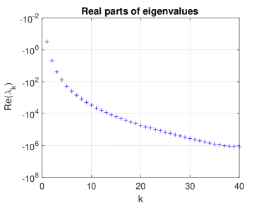
Based on this formula, the modal frequencies, real parts of the eigenvalues, and the ratios of the subsequent real parts are shown as a function of the mode number in Figure 6.

(a)

(b)

(c)

Figure 6: Spectral quotient analysis: the approximate ratio (15) between the real parts of successive eigenvalues of the system (c) reveals the spectral quotient gaps in the system. The first few eigen-modes form a subspace much slower than the rest and hence are relavant for the SSM reduction. No such large spectral gaps can be identified from the plots of the undamped natural frequencies (a) and real parts of the eigenvalues (b).

Note that the first eigenspace is about $16$ times slower in terms of its exponential decay rate than the second slowest eigenspace, which renders the first mode an optimal choice for reduction using its corresponding SSM. We will, therefore, use this mode to perform a single-mode SSM reduction for the beam model, as discussed below.

4.2 SSM-based reduction

In order to perform a further reduction of the reduced system (11) obtained from SFD, we now compute the slowest single-mode SSM, whose reduced dynamics is given by a two-dimensional ODE as a final reduced-order model. Szalai et al. [6] have obtained general formulae for such one-mode SSMs and their associated backbone curves for autonoumous dynamical systems (no external forcing in our setting). The reduced-order model obtained in this fashion is given in terms of an internal parametrization of the SSM, rather than a projection of the SSM on its underlying modal subspace. This construct allows the SSM to be recovered more globally, even if it develops a fold over the underlying modal subspace.

For this general formulation, we require the autonomous counterpart of system (11) to be in the phase space form

$$\underbrace{\left[\begin{array}[]{c}\dot{\mathbf{x}}\\ \ddot{\mathbf{x}}\end{array}\right]}_{\dot{\mathbf{\tilde{z}}}} =\underbrace{\left[\begin{array}[]{cc}\mathbf{0}&\mathbf{I}\\ -\mathbf{M}_{1}^{-1}\mathbf{K}_{1}&-\epsilon\zeta\mathbf{M}_{1}^{-1}\mathbf{K}_{1}\end{array}\right]}_{\mathbf{A}}\underbrace{\left[\begin{array}[]{c}\mathbf{x}\\ \dot{\mathbf{x}}\end{array}\right]}_{\mathbf{\tilde{z}}}+\mathbf{t}(\mathbf{x},\dot{\mathbf{x}})\,,$$ (22)

$$\mathrm{or}\quad\dot{\mathbf{\tilde{z}}} =\mathbf{A}\tilde{\mathbf{z}}+\mathbf{t}(\tilde{\mathbf{z}})\,,$$ (23)

where $\mathbf{t}(\mathbf{x},\dot{\mathbf{x}})$ is a class $C^{r}$ function representing the nonlinear terms in the ROM (11). By inspection of (11), we find that $\mathbf{t}$ is a strictly cubic polynomial in $\mathbf{\tilde{z}}$ and hence belongs to the class $C^{a}$ of analytic functions. The system (23) can be diagonalized as

$$\dot{\mathbf{z}}=\mathbf{\boldsymbol{\Lambda}}\mathbf{z}+\boldsymbol{\mathcal{T}}\left(\mathbf{z}\right),\quad\mathbf{z}\in\mathbb{C}^{2n_{s}},\quad\mathbf{\Lambda}=\mathrm{diag}\left(\lambda_{1},\dots,\,\lambda_{2n_{s}}\right),\,\lambda_{2i-1}=\bar{\lambda}_{2i},\,i\in\{1,\dots,\,n_{s}\},\quad\boldsymbol{\mathcal{T}}(\mathbf{z})=\mathcal{O}\left(|\mathbf{z}|^{3}\right)\,,$$ (24)

where $\lambda_{i}\in\mathbb{C\,}$ are the eigenvalues of the matrix $\mathbf{A}$ ordered such that $\mathrm{Re}\left(\lambda_{n_{s}}\right)\leq\dots\leq\mathrm{Re}\left(\lambda_{1}\right)<0$. The matrix $\mathbf{P}$ of the linear transformation $\mathbf{z}=\mathbf{P}^{-1}\tilde{\mathbf{z}}$ leading to (24), contains the corresponding eigenvectors of $\mathbf{A}$.

The notion of an SSM was introduced by Haller and Ponsioen [4], more formally defined as follows:

Definition 1.

A spectral submanifold (SSM), $W(\mathcal{E})$, corresponding to a spectral subspace $\mathcal{E}$ of $\mathbf{\Lambda}$ is an invariant manifold of the dynamical system (24) such that

(i)

$W(\mathcal{E})$ is tangent to $\mathcal{E}$ at the origin and has the same dimension as $\mathcal{E}$;

(ii)

$W(\mathcal{E})$ is strictly smoother than any other invariant manifold satisfying (i).

When $\boldsymbol{\mathcal{T}}\left(\mathbf{z}\right)$ is a $C^{r}$ function, then under the assumptions

(B1)

the relative spectral quotient $\sigma(\mathcal{E}):=\mathrm{Int}\left[\frac{\min_{j\neq\ell,\ell+1}\mathrm{Re}(\lambda_{j})}{\mathrm{Re}(\lambda_{\ell})}\right]$ satisfies $\sigma(\mathcal{E})\leq r$,

(B2)

there are no resonances up to order $\sigma(\mathcal{E})$ between $\lambda_{\ell},\,\bar{\lambda}_{\ell}$ and the rest of the spectrum of $\mathbf{\Lambda}$,

the existence and uniqueness of a class $C^{r+1}$ SSM is guaranteed by the main theorem of Haller and Ponsioen [4], deduced from the more general results of Cabré et al. [8]. The theorem states that the SSM can be viewed as an embedding of an open set $\mathcal{U}\subset\mathbb{C}^{2}$ into the phase space of system (24), described by a map $\mathbf{W}:\mathcal{U}\subset\mathbb{C}^{2}\mapsto\mathbb{C}^{2n_{s}}$. Furthermore, there exists a quadratic polynomial mapping $\mathbf{R}:\mathcal{U}\mapsto\mathcal{U}$, such that the reduced dynamics on the SSM can be written as

$$\dot{\mathbf{s}}=\mathbf{R\left(s\right)},\qquad\mathbf{R\left(s\right)}=\begin{bmatrix}\lambda_{\ell}z_{\ell}+\beta_{\ell}z_{\ell}^{2}\bar{z}_{\ell}\\ \bar{\lambda}_{\ell}\bar{z}_{\ell}+\bar{\beta}_{\ell}z_{\ell}\bar{z}_{\ell}^{2}\end{bmatrix},$$ (25)

where $\mathbf{s}=(z_{\ell},\bar{z}_{\ell})$ are the coordinates for the mode $\ell$ (for which the SSM construction is performed).

In our beam setting, we obtain $\sigma(\mathcal{E})=\frac{\omega_{0n_{s}}^{2}}{\omega_{0\ell}^{2}}+\mathcal{O}(\epsilon)$ from the eigenvalue approximation in (15). This shows that the relative spectral quotient $\sigma(\mathcal{E})$ depends on the chosen discretization and monotonically increases with the number of discretization variables. This can be expected physically from a proportionally damped mechanical structure in which the damping for the modes is expected to increase monotonically with the corresponding oscillation frequency. Since $\mathbf{g}\in C^{a}$ here, we obtain that (B1) is satisfied. Furthermore, we assume generic parameter values under which the non-resonance requirement (B2) is satisfied by the beam system. The theorem of Haller and Ponsioen [4] then applies to the system (24), and the formulae obtained by Szalai et al. [6] yield the coefficients of $\mathbf{R}$ and the quadratic and cubic Taylor coefficients of $\mathbf{W}$. Specifically, let $\boldsymbol{\mathcal{T}}$ be expanded in indicial notation as

$$\left(\mathbf{\boldsymbol{\mathcal{T}}}(\mathbf{z})\right)_{i}=\sum_{j=1}^{2n_{s}}\sum_{k=1}^{2n_{s}}\sum_{l=1}^{2n_{s}}T_{ijkl}z_{j}z_{k}z_{l}\quad\forall i,j,k,l\in{1,\dots,2n_{s}}\,,$$ (26)

and let $\mathbf{W}(\mathbf{s})$ be of the polynomial form

$$\mathbf{W}(\mathbf{s})=\mathbf{\boldsymbol{\mathcal{W}}}^{(1)}(\mathbf{s})+\mathbf{\boldsymbol{\mathcal{W}}}^{(2)}(\mathbf{s})+\boldsymbol{\mathcal{W}}^{(3)}(\mathbf{s})+\dots,$$ (27)

where $\mathbf{\boldsymbol{\mathcal{W}}}^{(n)}(\mathbf{s})$ denotes the $n^{\mathrm{th}}$order terms of $\mathbf{W}$.

The first-order terms in this expansion are given by

$$\mathbf{\boldsymbol{\mathcal{W}}}^{(1)}(\mathbf{s})=\mathbf{W}^{(1)}\mathbf{s}\,,$$

where $\mathbf{W}^{(1)}\in\mathbb{C}^{2n_{s}\times 2}$ is an all-zero matrix except for two non-zero entries given by $\left(\mathbf{W}^{(1)}\right)_{1,\ell}=\lambda_{\ell},\,\left(\mathbf{W}^{(1)}\right)_{2,\ell+1}=\lambda_{\ell+1}$. The $i^{\mathrm{th}}$ component of the quadratic terms can be written as

$$\left(\mathbf{\boldsymbol{\mathcal{W}}}^{(2)}(\mathbf{s})\right)_{i}=\sum_{j=1}^{2}\sum_{k=1}^{2}W_{ijk}^{(2)}s_{j}s_{k}\equiv 0\,,\quad i\in\{1,\dots,2n_{s}\},\quad j,k\in\{1,2\}\,,$$

where $\mathbf{W}^{(2)}\in\mathbb{C}^{2n_{s}\times 2\times 2}$ is an all-zero 3-tensor since $\boldsymbol{\mathcal{T}}$ has no quadratic components. Finally, using the formulae derived by Szalai et al. [6], we can write the cubic terms as

$$\left(\mathbf{\boldsymbol{\mathcal{W}}}^{(3)}(\mathbf{s})\right)_{i}=\sum_{j=1}^{2}\sum_{k=1}^{2}\sum_{l=1}^{2}W_{ijkl}^{(3)}s_{j}s_{k}s_{l}\,,\quad i\in\{1,\dots,2n_{s}\},\quad j,k,l\in\{1,2\}\,,$$

where $\mathbf{W}^{(3)}\in\mathbb{C}^{2n_{s}\times 2\times 2\times 2}$ is a sparse 4-tensor with nonzero entries given as

$$W_{i111}^{(3)} =\frac{T_{i\ell\ell\ell}}{3\lambda_{\ell}-\lambda_{i}}\,,\quad i\in\{1,\dots,2n_{s}\}\,,$$

$$W_{i222}^{(3)} =\frac{T_{i(\ell+1)(\ell+1)(\ell+1)}}{3\lambda_{\ell+1}-\lambda_{i}}\,,\quad i\in\{1,\dots,2n_{s}\}\,,$$

$$W_{ijkl}^{(3)} =(1-\delta_{i\ell})\frac{T_{ijkl}}{2\lambda_{\ell}+\bar{\lambda}_{\ell}-\lambda_{i}}\,,\quad i\in\{1,\dots,2n_{s}\},\quad(j,k,l)\in\{(\ell,\ell+1,\ell),(\ell,\ell,\ell+1),(\ell+1,\ell,\ell)\}\,,$$

$$W_{ijkl}^{(3)} =(1-\delta_{i(\ell+1)})\frac{T_{ijkl}}{2\lambda_{\ell+1}+\bar{\lambda}_{\ell+1}-\lambda_{i}}\,$$

$$\quad i\in\{1,\dots,2n_{s}\},\quad(j,k,l)\in\{(\ell+1,\ell,\ell+1),(\ell+1,\ell+1,\ell),(\ell,\ell+1,\ell+1)\}\,.$$

Here $T_{ijkl}\in\mathbb{C}$ denotes the components of the 4-tensor in the expansion of $\boldsymbol{\mathcal{T}}$ given in (26), and $\delta_{ij}$ respresents the Kronecker-delta. The expression for $\beta_{\ell}$ used in the expansion of $\mathbf{R}$ as in (25) is given by

$$\beta_{\ell}=T_{\ell\ell\ell(\ell+1)}+T_{\ell\ell(\ell+1)\ell}+T_{\ell(\ell+1)\ell\ell},$$

as obtained from the general formulae of Szalai et al. [6], reproduced in the B. Note that the Einstein summation convention has not been followed in the above expressions. We finally express the reduced dynamics in the polar coordinates $\left(\rho,\theta\right)$ using a transformation $\boldsymbol{\mathcal{R}}:\mathbb{\mathbb{C}}^{2}\mapsto\mathbb{R}\times\mathbb{S}^{1}$ such that $\mathbf{s}=\boldsymbol{\mathcal{R}}^{-1}\left(\rho,\theta\right)=\left(\rho e^{i\theta},\rho e^{-i\theta}\right)$, given by

$$\dot{\rho} =\rho(\mathrm{Re}\lambda_{\ell}+\mathrm{Re}\beta_{\ell}\rho^{2})\,,$$

$$\dot{\theta} =\mathrm{Im}\lambda_{\ell}+\mathrm{Im}\beta_{\ell}\rho^{2}\,.$$ (28)

4.3 Results

We now consider the SFD-reduced beam system (11) with the physically relevant parameter value $\epsilon=10^{-3}$, and further reduce it to its slowest, two-dimensional SSM with $\ell=1$. Let the modal coordinates be partitioned such that $Q_{1}(\mathbf{z}(\tau))=(z_{1}(\tau),\,z_{2}(\tau))$ represents the displacement of master modes, and $Q_{2}(\mathbf{z}(\tau))=(z_{3},\dots,z_{2n_{s}})$ represents the rest of the slow modes obtained previously from the SFD. For the two-dimensional SSM over longer time-scales, free oscillations of the beam are expected to decay towards the origin. To illustrate this over longer time scales, we consider three sets of intial conditions.

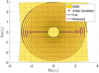
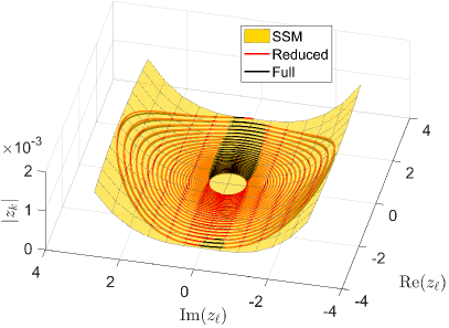
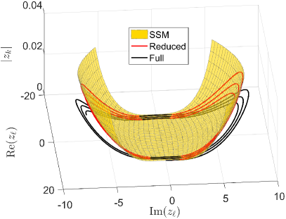
1. Initial condition on the SSM: Starting with an initial condition on the two-dimensional SSM, we observe in Figure 7a that the full solution indeed stays on the SSM, thereby showing that the SSM is indeed invariant. Since the computed $\mathbf{W}$ is only a third-order appoximation of the SSM, an initial condition far enough from the the fixed point may not stay over this approximate surface (cf. Figure 7b). Indeed, a higher-order approximation to $\mathbf{W}$ would be required to verify the invariance of $W(\mathcal{E})$ numerically for larger initial conditions.

   

   (a) Initial condition with polar coordinates $(\rho(0),\theta(0))=(3,0)$

   

   (b) Initial condition with polar coordinates $(\rho(0),\theta(0))=(9.0)$

   Figure 7: The SSM plotted in the modal coordinates $\mathbf{z}$. Full solution trajectory is shown for an initial condition taken on the SSM. Modal amplitude $|z_{k}|$ of the $k^{\mathrm{th}}$ mode ($k=3$) is plotted against the master modal variables ($\mathrm{Re}(z_{\ell}),\,\mathrm{Im}(z_{\ell})$) with $\ell=1$. The full solution trajectory (a) stays approximately on the computed SSM, (b) does not stay exactly on the computed SSM for an initialization far enough from the fixed point.

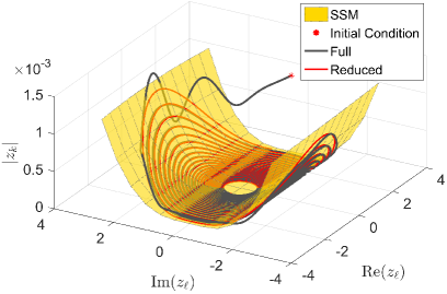
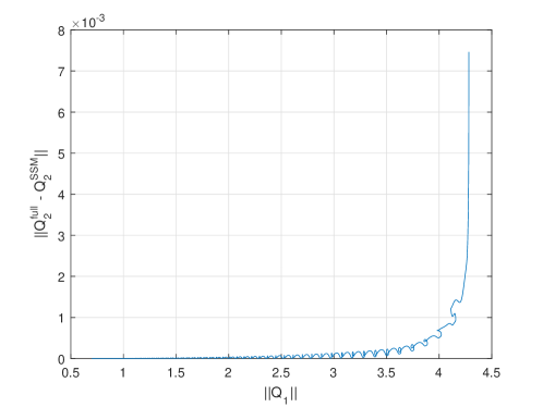
2. Initial condition off the SSM but still on the slow manifold: We illustrate that the SSM is attracting nearby trajectories within the SFD-based slow manifold by launching a trajectory away from the SSM but still inside the slow manifold $\mathcal{M}_{\epsilon}(\tau)$. As shown in Figure 8, a trajectory of the full solution which starts at an arbitrarily chosen point in the phase space of system (23), close enough to the computed SSM, quickly converges towards the SSM and synchronizes with the flow on the SSM. Figure 9 shows that this rate of attraction towards the SSM is indeed faster than the typical decay rate within the SSM.

   

   (a)

   

   (b)

   Figure 8: The SSM plotted in the modal coordinates $\mathbf{z}$. Full solution trajectory is shown for an initial condition taken off the SSM but still inside the slow manifold. Modal amplitude $|z_{k}|$ of the $k^{\mathrm{th}}$ mode ($k=3$) is plotted against the master modal unknows ($\mathrm{Re}(z_{\ell}),\,\mathrm{Im}(z_{\ell})$). The full solution trajectory (a) quickly decays onto the SSM, and (b) synchronises with the dynamics on the SSM.

   

   Figure 9: The exponential decay of trajectories towards the SSM within the slow manifold in the modal phase space: $|Q_{2}(\mathbf{z})-Q_{2}(\mathbf{W}(\mathbf{s}))|$ vs. $|Q_{1}(\mathbf{z}))|$. The decay rate transverse to the SSM is exponentially faster than that the typical rates along the SSM.

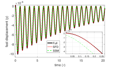
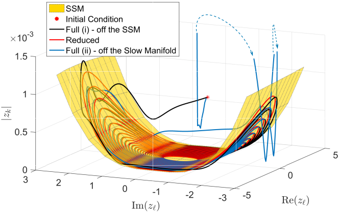
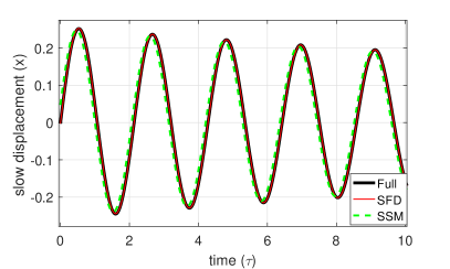
3. Initial condition off the slow manifold: Although the SSM is computed for the SFD-reduced system (11), the reduced dynamics on the SSM also captures the asymptotic behavior of the full system by construction. Indeed, as seen in Figure 10, a trajectory initialized off the slow manifold in the phase space of system (4) (thus off the SSM as well) is also attracted towards the SSM, and synchronizes with the corresponding flow on the SSM. This synchronization can be seen in more detail in Figure 11, where the time histories of slow and fast variables are compared between the slow and full solution. As expected, the response of the fast degree of freedom, in particular, shows that the full solution performs rapid oscilations around, and stabilizes on, the reduced solution obtained from SFD. Finally, the full solution approaches the SSM-reduced solution.

   

   Figure 10: Modal amplitude $|z_{k}|$ of the $k^{\mathrm{th}}$ mode ($k=3$) is plotted against the master modal variables ($\mathrm{Re}(z_{\ell}),\,\mathrm{Im}(z_{\ell})$). The full (ii) solution trajectory (blue) initialized off the slow manifold synchronizes with the reduced dynamics on the SSM. The full (i) soluion trajectory (black) is initialized on the slow manifold by projecting the original initial confition onto the slow manifold. Note that in this plot, the two initial conditions appear to coincide, since the axes feature only the slow (modal) DOFs. The dashed lines are a schematic representation of the trajectory leaving and returning to the plot region.

   

   (a)

   

   (b)

   Figure 11: The comparison of full and different reduced solutions for (a) slow and (b) fast degrees of freedom. Note the two timescales in the zoom-in for the dynamics of the fast DOF. The full solution quickly decays to the slow manifold (with SFD-reduced solutions) after which it decays to the SSM.

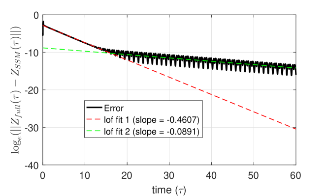
Next, we study the rate of decay of the enslaved variables towards the computed SSM. From Figure 12, we see that the initial decay rate of a trajectory towards the SSM is approximately $e^{-0.4607\tau}$ which is actually dominated by the decay rate suggested by the second slowest eigenvalue, i.e., $\mathrm{Re}(\lambda_{2})\approx-0.4724$. The slow dynamics within the SSM is expected to occur at the rate suggested by the first eigenvalue, i.e., $\mathrm{Re}(\lambda_{1})\approx-0.0295$. The final decay-rate for the full solution is, however, a decay rate of $e^{-0.0891\tau}$ which is between the slowest and second slowest rates, still being an order of magnitude faster than the dynamics within the SSM, as expected from the underlying theory.

Figure 12: The logarithmic plot shows $|\mathbf{z}(\tau)-\mathbf{W}(\mathbf{s}(\tau))|$ vs. time. The two fits suggest initial and final decay rates of $e^{-0.4607\tau}$ and $e^{-0.0891\tau}$ approximately, respectively. The approximate decay rates along and transverse to the SSM near the equilibrium are given by $e^{-0.0295\tau}$ and $e^{-0.4724\tau}$, respectively (based on the eigenvalues of the linearized system).

5 Conclusions

We have demonstrated two exact model reduction techniques, the slow-fast decomposition (SFD) and spectral-submanifold (SSM)-based reduction, on the finite-element model of a von Kármán beam. The SFD enabled us to express the fast axial variables of the beam as a graph over the slow transverse variables, yielding a reduced-order model only in terms of the slow variables. This SFD-reduced model possesses a gap in its spectral quotient disctribution, indicating an opportunity for further reduction using the SSM. Subsequently, we carried out a single-mode SSM-based reduction on the SFD-reduced model. This two-stage, exact reduction procedure resulted in a drastic reduction of the model dimension, and ensured that the full system trajectories synchronized with the reduced model trajectories at rates much faster than typical decay rates within the manifold.

The application of the above mentioned exact reduction techniques to our beam model confirms their potential for truly high-dimensional systems. However, significant work remains to be done to enable application of these techniques to simulations of realistic structures, especially on the computational implementation side. In particular, these techniques, in their present form, require the nonlinear coefficients of the system to be known apriori. For finite-element-based applications, often these nonlinear coefficients are embedded in the software at the element level and their full counterparts are never calculated during a simulation (for reasons of computational efficiency). This is certainly a computational challenge for application of SFD/SSM-based reduction techniques to real-world applications and shall be the focus of our future endeavours.

The current work features a single-mode SSM. This was justified in our beam example, because decay rates in the first mode were exceptionally slower than the rest. For more general damped-mechanical systems, however, we expect higher-dimensional SSMs (i.e., smoothest nonlinear continuations of high-dimensional linear modal subspaces) to be more relevant for reduction. Furthermore, the polynomial expansion of the SSM mapping contains terms only up to the third order in the current work. As also discussed in Section 4.3, higher-order terms would play an important role in capturing trajectories initialized farther from the fixed point. A MATLAB computational toolbox to compute multi-mode SSMs with terms of up to arbitrary order is currently under development (cf. Ponsioen and Haller [22]).

The current work covers the autonomous (non-forced) beam model. Existence and uniqueness results for SSMs are also available for non-autonomous, damped mechanical systems as discussed by Haller and Ponsioen [4]. For (quasiperiodically) forced systems, the SSM appears as a quasiperiodically deforming invariant surface in the phase space, which is again an ideal tool for model reduction. The computation of such non-autonomous SSMs will find useful application in non-autonomous mechanical systems, and is subject to ongoing work (cf. Breunung and Haller [23]).

Appendix A $\mathcal{O}\left(\epsilon^{2}\right)$terms in the slow manifold

As shown by Haller and Ponsioen [3], the enslavement of the fast variables to the slow ones along the slow manifold is given by the functions

$$\mathbf{y} =\epsilon\mathbf{G}_{0}(\mathbf{x},\dot{\mathbf{x}},\tau)+\epsilon^{2}\mathbf{G}_{1}(\mathbf{x},\dot{\mathbf{x}},\tau)+\epsilon^{3}\mathbf{G}_{2}(\mathbf{x},\dot{\mathbf{x}},\tau)+\mathcal{O}\left(\epsilon^{4}\right)\,,$$

$$\dot{\mathbf{y}} =\epsilon\mathbf{H}_{0}(\mathbf{x},\dot{\mathbf{x}},\tau)+\epsilon^{2}\mathbf{H}_{1}(\mathbf{x},\dot{\mathbf{x}},\tau)+\epsilon^{3}\mathbf{H}_{2}(\mathbf{x},\dot{\mathbf{x}},\tau)+\mathcal{O}\left(\epsilon^{4}\right)\,,$$

where $\mathbf{G}_{0},\,\mathbf{G}_{1},\,\mathbf{H}_{0}$ are as shown in (12) and $\mathbf{H}_{1}$ is given by

$$\mathbf{H}_{1}(\mathbf{x},\dot{\mathbf{x}},\tau)=\left[\partial_{\mathbf{x}}\mathbf{G}_{1}\right]\dot{\mathbf{x}}+\left[\partial_{\dot{\mathbf{x}}}\mathbf{G}_{1}\right]\overline{\mathbf{P}_{1}}+\partial_{\tau}\mathbf{G}_{1}+\partial_{\dot{\mathbf{x}}}\mathbf{G}_{0}\left(\overline{\partial_{\boldsymbol{\eta}}\mathbf{P}_{1}}\mathbf{G}_{1}+\overline{\partial_{\dot{\mathbf{y}}}\mathbf{P}_{1}}\mathbf{H}_{0}+\overline{\partial_{\epsilon}\mathbf{P}_{1}}\right).$$ (29)

In order to obtain the $\mathcal{O}\left(\epsilon^{2}\right)$ terms in the reduced model, we have calculated the general expressions for $\mathbf{G}_{2}$ as

$$\mathbf{G}_{2}(\mathbf{x},\dot{\mathbf{x}},\tau) =\left[\overline{\partial_{\boldsymbol{\eta}}\mathbf{P}_{2}}\right]^{-1}\left(\left[\partial_{\mathbf{x}}\mathbf{H}_{0}\right]\dot{\mathbf{x}}+\left[\partial_{\dot{\mathbf{x}}}\mathbf{H}_{0}\right]\overline{\mathbf{P}_{1}}+\partial_{\tau}\mathbf{H}_{0}-\left(\mathbf{J}\mathbf{G}_{1}+\mathbf{L}\mathbf{H}_{0}+\overline{\partial_{\epsilon}^{2}\mathbf{P}_{2}}+\overline{\partial_{\dot{\mathbf{y}}}\mathbf{P}_{2}}\mathbf{H}_{1}\right)\right),$$ (30)

where

$$\mathbf{J} =\frac{1}{2}\left(\overline{\partial_{\boldsymbol{\eta}}^{2}\mathbf{P}_{2}}\mathbf{G}_{1}+\overline{\partial_{\dot{\mathbf{y}}}\partial_{\boldsymbol{\eta}}\mathbf{P}_{2}}\mathbf{H}_{0}+\overline{\partial_{\epsilon}\partial_{\boldsymbol{\eta}}\mathbf{P}_{2}}\right)\,,$$

$$\mathbf{L} =\frac{1}{2}\left(\overline{\partial_{\dot{\mathbf{y}}}^{2}\mathbf{P}_{2}}\mathbf{H}_{0}+\overline{\partial_{\boldsymbol{\eta}}\partial_{\dot{\mathbf{y}}}\mathbf{P}_{2}}\mathbf{G}_{1}+\overline{\partial_{\epsilon}\partial_{\dot{\mathbf{y}}}\mathbf{P}_{2}}\right)\,.$$

The reduced-order model including the $\mathcal{O}\left(\epsilon^{2}\right)$ terms is then given as

$$\ddot{\mathbf{x}}-\overline{\mathbf{P}_{1}}-\epsilon\left[\overline{\partial_{\boldsymbol{\eta}}\mathbf{P}_{1}}\mathbf{G}_{1}+\overline{\partial_{\dot{\mathbf{y}}}\mathbf{P}_{1}}\mathbf{H_{0}}+\overline{\partial_{\epsilon}\mathbf{P}_{1}}\right]-\epsilon^{2}\left[\mathbf{N}\mathbf{G}_{1}+\overline{\partial_{\boldsymbol{\eta}}\mathbf{P}_{1}}\mathbf{G}_{2}+\mathbf{R}\mathbf{H}_{0}+\overline{\partial_{\dot{\mathbf{y}}}\mathbf{P}_{1}}\mathbf{H}_{1}+\overline{\partial_{\epsilon}^{2}\mathbf{P}_{1}}\right]+\mathcal{O}(\epsilon^{3})=\mathbf{0},$$

where

$$\mathbf{N} =\frac{1}{2}\left(\overline{\partial_{\boldsymbol{\eta}}^{2}\mathbf{P}_{1}}\mathbf{G}_{1}+\overline{\partial_{\dot{\mathbf{y}}}\partial_{\boldsymbol{\eta}}\mathbf{P}_{1}}\mathbf{H}_{0}+\overline{\partial_{\epsilon}\partial_{\boldsymbol{\eta}}\mathbf{P}_{1}}\right)\,,$$

$$\mathbf{R} =\frac{1}{2}\left(\overline{\partial_{\dot{\mathbf{y}}}^{2}\mathbf{P}_{1}}\mathbf{H}_{0}+\overline{\partial_{\boldsymbol{\eta}}\partial_{\dot{\mathbf{y}}}\mathbf{P}_{1}}\mathbf{G}_{1}+\overline{\partial_{\epsilon}\partial_{\dot{\mathbf{y}}}\mathbf{P}_{1}}\right)\,.$$

In our beam framework, the general expressions in (29,30) become

$$\mathbf{H}_{1}(\mathbf{x},\dot{\mathbf{x}},\tau) =\mathbf{K}_{2}^{-1}\left(\zeta\left[\partial_{\mathbf{x}}\boldsymbol{\mathcal{H}}(\mathbf{x})-\boldsymbol{\mathcal{E}}(\mathbf{x})\right]\overline{\mathbf{P}_{1}}+\zeta\left[\partial_{\mathbf{x}}^{2}\boldsymbol{\mathcal{H}}(\mathbf{x})-\partial_{\mathbf{x}}\boldsymbol{\mathcal{E}}(\mathbf{x})\right]:(\dot{\mathbf{x}}\otimes\dot{\mathbf{x}})+\beta\dot{\mathbf{p}}\right)\,,$$

$$\mathbf{G}_{2}(\mathbf{x},\dot{\mathbf{x}},\tau) =\left[\mathbf{K}_{2}\mathbf{M}_{2}^{-1}\mathbf{K}_{2}\right]^{-1}\left(\left[\partial_{\mathbf{x}}^{2}\boldsymbol{\mathcal{H}}(\mathbf{x})\right]:(\dot{\mathbf{x}}\otimes\dot{\mathbf{x}})+\left[\partial_{\mathbf{x}}\boldsymbol{\mathcal{H}}(\mathbf{x})\right]\overline{\mathbf{P}_{1}}\right)-\zeta\mathbf{H}_{1}.$$ (31)

For the assumed visco-elastic material damping, the expressions for $\mathbf{G}_{1}(\mathbf{x},\dot{\mathbf{x}},\tau)$ in (12) and $\mathbf{H}_{1}(\mathbf{x},\dot{\mathbf{x}},\tau)$ in (31) can be further simplified to

$$\mathbf{G}_{1}(\mathbf{x},\dot{\mathbf{x}},\tau) =\beta\mathbf{K}_{2}^{-1}\mathbf{p}(\tau)\,,$$

$$\mathbf{H}_{1}(\mathbf{x},\dot{\mathbf{x}},\tau) =\beta\mathbf{K}_{2}^{-1}\dot{\mathbf{p}}(\tau)\,,$$

and the reduced-order model can be simplified as

$$\mathbf{M}_{1}\ddot{\mathbf{x}}+\mathbf{K}_{1}\mathbf{x}+\boldsymbol{\mathcal{F}}\left(\mathbf{x},\mathbf{G}_{0}(\mathbf{x},\dot{\mathbf{x}},\tau)\right)+\boldsymbol{\mathcal{G}}(\mathbf{x})+$$

$$\epsilon\left[\overline{\partial_{\boldsymbol{\eta}}\boldsymbol{\mathcal{F}}\left(\mathbf{x},\boldsymbol{\eta}\right)}\mathbf{G}_{1}(\mathbf{x},\dot{\mathbf{x}},\tau)+\zeta\left(\boldsymbol{\mathcal{D}}(\mathbf{x})\mathbf{H}_{0}(\mathbf{x},\dot{\mathbf{x}},\tau)+\left(\mathbf{K}_{1}+\boldsymbol{\mathcal{C}}(\mathbf{x})\right)\dot{\mathbf{x}}\right)\right]+$$ (32)

$$\epsilon^{2}\left[\overline{\partial_{\boldsymbol{\eta}}\boldsymbol{\mathcal{F}}\left(\mathbf{x},\boldsymbol{\eta}\right)}\mathbf{G}_{2}(\mathbf{x},\dot{\mathbf{x}},\tau)+\zeta\boldsymbol{\mathcal{D}}(\mathbf{x})\mathbf{H}_{1}(\mathbf{x},\dot{\mathbf{x}},\tau)\right]+\mathcal{O}\left(\epsilon^{3}\right)=\alpha\mathbf{q}(\tau).$$

Appendix B Forumulae for single-mode SSMs

We express the general formulae of Szalai et al. [6] for Taylor coefficients of the SSM mapping $\mathbf{W}(\mathbf{s})$ in our present notation. Let $\boldsymbol{\mathcal{T}}(\mathbf{z})$ from (24) be a general polynomial of the form

$$\boldsymbol{\mathcal{T}}(\mathbf{z})=\mathbf{\boldsymbol{\mathcal{T}}}^{(2)}(\mathbf{z})+\mathbf{\boldsymbol{\mathcal{T}}}^{(3)}(\mathbf{z})+\dots,$$ (33)

where $\mathbf{\boldsymbol{\mathcal{T}}}^{(n)}(\mathbf{z})$ denotes the $n^{\mathrm{th}}$order terms of $\boldsymbol{\mathcal{T}}$. The first order terms in the expansion (27) are given by

$$\mathbf{\boldsymbol{\mathcal{W}}}^{(1)}(\mathbf{s})=\mathbf{W}^{(1)}\mathbf{s}\,,$$

where $\mathbf{W}^{(1)}\in\mathbb{C}^{2n_{s}\times 2}$ is an all-zero matrix except for two non-zero entries given by $\left(\mathbf{W}^{(1)}\right)_{1,\ell}=\lambda_{\ell},\,\left(\mathbf{W}^{(1)}\right)_{2,\ell+1}=\lambda_{\ell+1}$. The $i^{\mathrm{th}}$ component of the quadratic terms can be written as

$$\left(\mathbf{\boldsymbol{\mathcal{W}}}^{(2)}(\mathbf{s})\right)_{i}=\sum_{j=1}^{2}\sum_{k=1}^{2}W_{ijk}^{(2)}s_{j}s_{k}\,,\quad i\in\{1,\dots,2n_{s}\},\quad j,k\in\{1,2\}\,,$$

where $\mathbf{W}^{(2)}\in\mathbb{C}^{2n_{s}\times 2\times 2}$ is a sparse 3-tensor with nonzero entries given as

$$W_{i11}^{(2)} =\frac{T_{i\ell\ell}^{(2)}}{2\lambda_{\ell}-\lambda_{i}}\,,\quad i\in\{1,\dots,2n_{s}\}\,,$$

$$W_{i22}^{(2)} =\frac{T_{i(\ell+1)(\ell+1)}^{(2)}}{2\lambda_{\ell+1}-\lambda_{i}}\,,\quad i\in\{1,\dots,2n_{s}\}\,,$$

$$W_{ijk}^{(2)} =\frac{T_{ijk}^{(2)}}{\lambda_{\ell}+\bar{\lambda}_{\ell}-\lambda_{i}}\,,\quad i\in\{1,\dots,2n_{s}\},\quad(j,k)\in\{(\ell,\ell+1),(\ell+1,\ell)\}\,.$$

Finally, the cubic terms can be written as

$$\left(\mathbf{\boldsymbol{\mathcal{W}}}^{(3)}(\mathbf{s})\right)_{i}=\sum_{j=1}^{2}\sum_{k=1}^{2}\sum_{l=1}^{2}W_{ijkl}^{(3)}s_{j}s_{k}s_{l}\,,\quad i\in\{1,\dots,2n_{s}\},\quad j,k,l\in\{1,2\}\,,$$

where $\mathbf{W}^{(3)}\in\mathbb{C}^{2n_{s}\times 2\times 2\times 2}$ is a sparse 4-tensor with nonzero entries given as

$$W_{i111}^{(3)} =\frac{\sum_{j=1}^{2n_{s}}\left[\left(1+\delta_{\ell j}\right)\left(T_{ij\ell}^{(2)}+T_{i\ell j}^{(2)}\right)W_{j11}^{(2)}\right]+T_{i\ell\ell\ell}^{(3)}}{3\lambda_{\ell}-\lambda_{i}}\,,\quad i\in\{1,\dots,2n_{s}\}\,,$$

$$W_{i222}^{(3)} =\frac{\sum_{j=1}^{2n_{s}}\left[\left(1+\delta_{(\ell+1)j}\right)\left(T_{ij(\ell+1)}^{(2)}+T_{i(\ell+1)j}^{(2)}\right)W_{j22}^{(2)}\right]+T_{i(\ell+1)(\ell+1)(\ell+1)}^{(3)}}{3\lambda_{\ell+1}-\lambda_{i}}\,,\quad i\in\{1,\dots,2n_{s}\}\,,$$

$$W_{ijkl}^{(3)} =(1-\delta_{i\ell})\frac{V_{i}+T_{ijkl}^{(3)}}{2\lambda_{\ell}+\bar{\lambda}_{\ell}-\lambda_{i}}\,,\quad i\in\{1,\dots,2n_{s}\},\quad(j,k,l)\in\{(\ell,\ell+1,\ell),(\ell,\ell,\ell+1),(\ell+1,\ell,\ell)\}\,,$$

$$W_{ijkl}^{(3)} =(1-\delta_{i(\ell+1)})\frac{U_{i}+T_{ijkl}^{(3)}}{2\lambda_{\ell+1}+\bar{\lambda}_{\ell+1}-\lambda_{i}}\,$$

$$\quad i\in\{1,\dots,2n_{s}\},\quad(j,k,l)\in\{(\ell+1,\ell,\ell+1),(\ell+1,\ell+1,\ell),(\ell,\ell+1,\ell+1)\}\,,$$

with

$$V_{i} =\sum_{j=1}^{2n_{s}}\left[\left(1+\delta_{\ell j}\right)\left(T_{ij\ell}^{(2)}+T_{i\ell j}^{(2)}\right)\left(W_{j21}^{(2)}+W_{j12}^{(2)}\right)+\left(1+\delta_{(\ell+1)j}\right)\left(T_{ij(\ell+1)}^{(2)}+T_{i(\ell+1)j}^{(2)}\right)W_{j11}^{(2)}\right]\,,\quad i\in\{1,\dots,2n_{s}\},$$

$$U_{i} =\sum_{j=1}^{2n_{s}}\left[\left(1+\delta_{(\ell+1)j}\right)\left(T_{ij(\ell+1)}^{(2)}+T_{i(\ell+1)j}^{(2)}\right)\left(W_{j21}^{(2)}+W_{j12}^{(2)}\right)+\left(1+\delta_{\ell j}\right)\left(T_{ij\ell}^{(2)}+T_{i\ell j}^{(2)}\right)W_{j22}^{(2)}\right]\,,\quad i\in\{1,\dots,2n_{s}\}.$$

Here $T_{ijkl}^{(3)},T_{ijk}^{(2)}\in\mathbb{C}$ denote the components of the 4-tensor and 3-tensor, respectively, in the expansion of $\boldsymbol{\mathcal{T}}$ given in (33), and $\delta_{ij}$ respresents the Kronecker-delta. Furthermore, the general expression for $\beta_{\ell}$ used in the expansion for $\mathbf{R}$ as in (25), as derived by Szalai et al. [6], can be written in our notation as

$$\beta_{\ell}=V_{\ell}+T_{\ell\ell\ell(\ell+1)}+T_{\ell\ell(\ell+1)\ell}+T_{\ell(\ell+1)\ell\ell}.$$

Note that the Einstein summation convention has not been followed in any of the above expressions.

References

• [1] Reddy, J. N., An Introduction to Nonlinear Finite Element Analysis. Oxford Univeristy Press (2010), Print ISBN-13: 9780198525295. DOI:10.1093/acprof:oso/9780198525295.001.0001
• [2] Crisfield, M. A., Non-linear Finite Element Analysis of Solids and Structures - Volume 1, Wiley (1996), ISBN-978-0471970590.
• [3] Haller, G. and Ponsioen, S., Exact Model Reduction by a Slow-Fast Decomposition of Nonlinear Mechanical Systems. Submitted, arXiv:1611.06210 (2016).
• [4] Haller, G. & Ponsioen, S. Nonlinear normal modes and spectral submanifolds: existence, uniqueness and use in model reduction. Nonlinear Dyn (2016) 86: 1493. DOI:10.1007/s11071-016-2974-z.
• [5] Fenichel, N., Geometric singular perturbation theory for ordinary differential equations. J. Diff. Eqs. 31 (1979) 53-98. DOI: 10.1016/0022-0396(79)90152-9
• [6] Szalai R., Ehrhardt, D., Haller, G.,Nonlinear model identification and spectral submanifolds for multi-degree-of-freedom mechanical vibrations. Submitted, arXiv:1610.02252 (2016).
• [7] Géradin, M., and Rixen, D.J., Mechanical Vibrations: Theory and Application to Structural Dynamics, (3rd ed) Wiley (2015), ISBN: 978-1-118-90020-8.
• [8] Cabre, R. de la Llave X., Fontich.,E. The parameterization method for invariant manifolds I: Manifolds associated to non-resonant subspaces. Indiana Univ. Math. J. (2003) 52:283–328.
• [9] Kosambi, D. Statistics in function space, Journal of the Indian Mathematical Society, 7 (1943), pp. 76–78
• [10] Amabili, M., Sarkar, A., Paıdoussis, M.P. Reduced-order models for nonlinear vibrations of cylindrical shells via the proper orthogonal decomposition method. J Fluids Struct 18(2):227–250. DOI: 10.1016/j.jfluidstructs.2003.06.002
• [11] Kerschen, G., Golinval, J.C., Vakakis, A.F., Bergman, L.A. The method of proper orthogonal decomposition for dynamical characterization and order reduction of mechanical systems: an overview. Nonlinear Dyn (2005) 41(1–3):147–169. DOI:10.1007/s11071-005-2803-2
• [12] Guyan, R.J. Reduction of stiffness and mass matrices, AIAA Journal (1965) 3 (2), p. 380 DOI:10.2514/3.2874
• [13] Craig, R., Bampton, M. Coupling of substructures for dynamic analysis, AIAA Journal (1968), 6 (7), pp. 1313–1319. DOI: 10.2514/3.4741
• [14] Zhaojun, B. Krylov subspace techniques for reduced-order modeling of large-scale dynamical systems. Applied Numerical Mathematics (2002) 43(1-2) 9–44. DOI: 10.1016/S0168-9274(02)00116-2
• [15] Pesheck, E., Pierre, C., Shaw, S.W. A new Galerkin-based approach for accurate non-linear normal modes through invariant manifolds. J Sound Vib 249(5) (2002) 971–993. DOI: 10.1006/jsvi.2001.3914
• [16] Jain, S., Tiso, P., Rixen, D.J., Rutzmoser, J.B. A Quadratic Manifold for Model Order Reduction of Nonlinear Structural Dynamics, Submitted arXiv:1610.09902 (2016)
• [17] Rutzmoser, J.B., Rixen, D.J., Tiso, P., Jain, S. Generalization of Quadratic Manifolds for Reduced Order Modeling of Nonlinear Structural Dynamics, Submitted arXiv:1610.09906 (2016)
• [18] Lee, J.A., Verleysen, M. Nonlinear Dimensionality Reduction. Springer Publishing Company, Incorporated, Heidelberg (2007) ISBN: 978-0-387-39350-6 (Print) 978-0-387-39351-3 (Online), DOI 10.1007/978-0-387-39351-3
• [19] Mignolet, M.P., Przekop, A., Rizzi, S.A., Spottswood, S.M. A review of indirect/non-intrusive reduced order modeling of nonlinear geometric structures. J Sound Vib (2013) 332(10), 2437-2460. DOI: 10.1016/j.jsv.2012.10.017
• [20] Ilbeigi S., Chelidze D. Model Order Reduction of Nonlinear Euler-Bernoulli Beam. In: Kerschen G. (eds) Nonlinear Dynamics, Volume 1 (2016). Conference Proceedings of the Society for Experimental Mechanics Series. Springer, Cham. DOI: 10.1007/978-3-319-15221-9_34
• [21] Craig, R.R. and Ni, Z. Component mode synthesis for model order reduction of nonclassicallydamped systems, Journal of Guidance, Control, and Dynamics, (1989)12(4), 577-584. DOI:10.2514/3.20446
• [22] Ponsioen, S., Haller, G. A graphical user interface for computing Spectral Submanifolds in dynamical systems (in preparation)
• [23] Breunung, T., Haller, G. Computation of Spectral Submanifolds for non-autonomous mechanical systems (in preparation)
• [24] Shaw, S.W., Pierre,C. Normal Modes for Non-Linear Vibratory Systems, J Sound Vib (1993) 164(1), 85-124. DOI: 10.1006/jsvi.1993.1198
• [25] Kerschen, G. (ed.), Modal Analysis of Nonlinear Mechanical Systems. Springer, Berlin (2014). ISBN 978-1-84996-924-6. DOI 10.1007/978-1-4471-3827-3