Phase Transitions, Inhomogeneous Horizons and Second-Order Hydrodynamics

Abstract

We use holography to study the spinodal instability of a four-dimensional, strongly-coupled gauge theory with a first-order thermal phase transition. We place the theory on a cylinder in a set of homogeneous, unstable initial states. The dual gravity configurations are black branes afflicted by a Gregory-Laflamme instability. We numerically evolve Einstein’s equations to follow the instability until the system settles down to a stationary, inhomogeneous black brane. The dual gauge theory states have constant temperature but non-constant energy density. We show that the time evolution of the instability and the final states are accurately described by second-order hydrodynamics. In the static limit, the latter reduces to a single, second-order, non-linear differential equation from which the inhomogeneous final states can be derived.

I Introduction

Hydrodynamics is one of the most successful theories in physics, capable of describing the dynamics of very different systems over an enormous range of length scales. Traditionally, it is thought of as an effective theory for the conserved charges of a system, constructed as a derivative expansion around local thermal equilibrium. From this perspective hydrodynamics is only expected to be valid when these gradient corrections are small compared to all the microscopic scales. However, in recent years it has been discovered that the regime of validity is actually much broader.

From an experimental viewpoint, hydrodynamics has been extremely successful at describing the post-collision dynamics of the drops of matter produced in ultra-relativistic collisions of large nuclei at RHIC Ackermann:2000tr ; Adler:2003kt ; Back:2004mh and the LHC ATLAS:2012at ; Chatrchyan:2012ta ; Aamodt:2010pa ; Aamodt:2010pa . Multi-particle correlations in these collisions are well described by hydrodynamics Huovinen:2001cy ; Teaney:2001av ; Hirano:2005xf ; Luzum:2008cw ; Schenke:2010rr ; hiranoLHC ; Shen:2014vra ; Bernhard:2016tnd , provided one assumes that the latter is valid in the presence of large gradients Romatschke:2016hle . Also, the recent finding of similar correlations in even smaller proton-proton collisions Khachatryan:2010gv ; Aad:2015gqa ; Khachatryan:2016txc provides a strong indication that hydrodynamics is applicable even at a baryonic scale Bozek:2011if ; Schenke:2014zha ; Kozlov:2014fqa ; Weller:2017tsr . From a theoretical viewpoint, studies of non-abelian gauge theories have shown that hydrodynamics is valid for systems with large gradients both at strong Chesler:2010bi ; Heller:2011ju ; Casalderrey-Solana:2013aba ; Chesler:2016ceu ; Attems:2016tby and weak coupling Kurkela:2015qoa ; Keegan:2016cpi .

In this paper we use the gauge/string duality to test the validity of hydrodynamics in a theory with a first-order thermal phase transition. We place the theory on a cylinder in a variety of homogeneous, unstable initial states. In the gauge theory the instability is a spinodal instability associated to the presence of a first-order phase transition. On the gravity side the instability is a long-wave length, Gregory-Laflamme-type instability Gregory:1993vy . We use the gravity description to follow the evolution of these states until they settle down to a stationary, inhomogeneous final state. We then compare both the time evolution and the final configurations to the corresponding hydrodynamic predictions. Recent related work includes Janik:2015iry ; Gursoy:2016ggq ; Dias:2017uyv .

To the best of our knowledge, from the boundary theory viewpoint our results provide the first example of a first-principle, non-perturbative, complete dynamical evolution of a spinodal instability in a strongly coupled gauge theory. From the gravity viewpoint, they provide the first example of the full dynamical evolution of a Gregory-Laflamme-type instability in an asymptotically anti-de Sitter space.

II Model

Motivated by simplicity, we study the Einstein-plus-scalar model with action

$$S=\frac{2}{\kappa_{5}^{2}}\int d^{5}x\sqrt{-g}\left[\frac{1}{4}{\mathcal{R}}-\frac{1}{2}\left(\nabla\phi\right)^{2}-V(\phi)\right].$$ (1)

The potential is

$$\ell\,V=-3-\frac{3\phi^{2}}{2}-\frac{\phi^{4}}{3}-\frac{\phi^{6}}{3\phi_{M}^{2}}+\frac{\phi^{6}}{2\phi_{M}^{4}}-\frac{\phi^{8}}{12\phi_{M}^{4}}$$ (2)

with $\ell$ the asymptotic curvature radius and $\phi_{M}=2.3$. The dual gauge theory is a Conformal Field Theory (CFT) deformed with a dimension-three scalar operator with source $\Lambda$, which appears as a boundary condition for the scalar. This is exactly the potential of Attems:2016ugt except for the sign reversal of the fourth term in $V$. This difference has dramatic implications for the thermodynamics of the gauge theory, which we extract from the homogeneous black brane solutions of the gravity model. In particular, the gauge theory possess a first-order phase transition at a critical temperature $T_{c}=0.247\Lambda$, as illustrated by the multivalued plot of the energy density as a function of the temperature in Fig. 1. States on the dashed red curve are locally thermodynamically unstable since the specific heat is negative, $c_{v}=d{\mathcal{E}}/dT<0$. In this region the speed of sound, $c_{s}^{2}=s/c_{v}$, with $s$ the entropy density, becomes imaginary. This leads to a dynamical, spinodal instability (see e.g. Chomaz:2003dz ) whereby the amplitude of small sound excitations grows exponentially with a momentum-dependent growth rate dictated by the sound dispersion relation:

$$\Gamma(k)\simeq\left|c_{s}\right|k-\frac{1}{2T}\left(\frac{4}{3}\frac{\eta}{s}+\frac{\zeta}{s}\right)k^{2}\,,$$ (3)

where $\eta$ and $\zeta$ are the shear and bulk viscosities. In our model $\eta/s=1/4\pi$ Kovtun:2004de and we compute $\zeta$ numerically following Eling:2011ms .

The corresponding statement on the gravity side is that the black branes dual to the states on the dashed red curve are afflicted by a long-wave length instability. Although this is similar to the Gregory-Laflamme instability of Ref. Gregory:1993vy , we will see below that there are also crucial differences between the two.

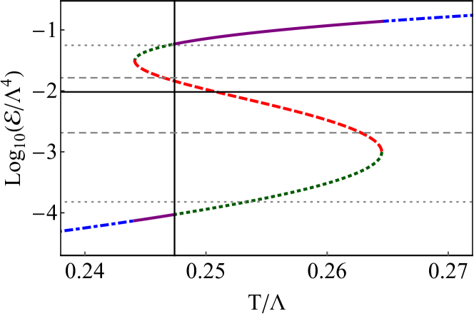
Figure 1: Energy density versus temperature for the gauge theory dual to (1). At high and low $T$ there is only one phase shown in dashed-dotted blue. The preferred phase in the multivalued region is shown in solid purple. The dotted green curve is metastable. The dashed red curve is locally unstable. The black vertical line indicates $T_{c}=0.247\Lambda$. The top (bottom) dashed, grey horizontal line indicates the highest (lowest) average energy density that we have considered. The top (bottom) dotted, grey horizontal line indicates the maximum (minimum) value of the energy in the corresponding final states. The solid, black horizontal line is the state for which we show specific results.

III Inhomogeneous horizon

To investigate the fate of the spinodal instability we compactify the gauge theory direction $z$ on a circle of length $L\simeq 57/\Lambda$. This infrared cut-off reduces the number of unstable sound modes to a finite number. We then consider a set of homogeneous, unstable initial states with energy densities in the range $\mathcal{E}/\Lambda^{4}\simeq(0.002,0.016)$, as indicated by the grey, dashed horizontal lines in Fig. 1. For concreteness we will show results for the state with $\mathcal{E}/\Lambda^{4}\simeq 0.0096$, whose temperature and entropy density are $T_{i}\simeq 0.251\Lambda$ and $s_{i}=0.037\Lambda^{3}$. To trigger the instability, we introduce a small $z$-dependent perturbation in the energy density corresponding to a specific Fourier mode on the circle. For concreteness we will show results for the case with $k=3(2\pi/L)\simeq 1.3T_{i}$. This mode is unstable with positive growth rate $\Gamma=0.0247\,\Lambda$ according to (3). For numerical simplicity we impose homogeneity along the transverse directions.

On the gravity side the sound-mode instability may be viewed Buchel:2005nt ; Emparan:2009cs ; Emparan:2009at as a Gregory-Laflamme instability Gregory:1993vy . We follow it by numerically evolving the Einstein-plus-scalar equations as in Attems:2016tby ; Attems:2017zam until the system settles down to a state with an inhomogeneous Killing horizon with constant temperature $T_{f}=0.250\Lambda$. Note that this is close but not identical to $T_{i}$ or $T_{c}$.

Figure 2: Energy density for the initial state indicated by the solid, black horizontal line in Fig. 1, perturbed by the third Fourier mode. The color coding on the final-time slice is the same as in Fig. 1.

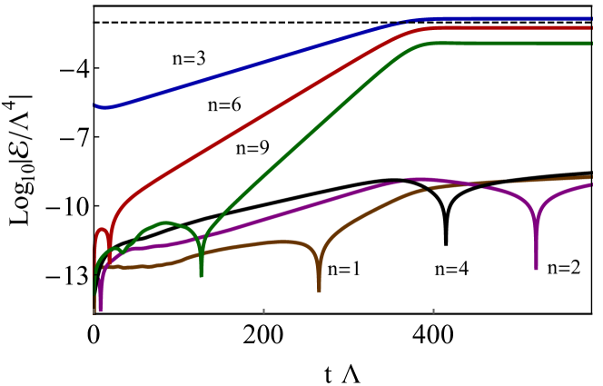
Figure 3: Time evolution of some Fourier modes of the energy density ${\mathcal{E}}$. The dashed horizontal line is the average energy density.

From the dynamical metric we extract the boundary stress tensor. The result for the energy density is shown in Fig. 2. The time dependence of the amplitudes of several modes of the energy density is shown in Fig. 3. The $n=3$ mode grows with a rate that agrees with (3) within 4%. Resonant behavior makes the modes with $n=6,9,\ldots$ grow at a rate that is roughly the corresponding multiple of the $n=3$ rate. Numerical noise makes some non-multiples of the $n=3$ mode (of which only three are shown in the figure) grow too. At late times the non-linear dynamics stops the growth of all these modes and the system settles down to a stationary, inhomogeneous configuration consisting of three identical domains. The fact that their size is comparable to the inverse temperature, $\Delta z=L/3\simeq 0.4/T_{f}$, is our first indication that spatial gradients are large.

In Fig. 4 we show the final entropy density as extracted from the area of the horizon. The fact that $s$ is not constant proves that the horizon itself (not just the boundary energy density) is inhomogeneous. We see in the figure that $s$ is very well estimated by a point-wise application of the equation of state to the final energy density of Fig. 2, suggesting that the evolution is quasi-adiabatic. This is confirmed by the fact the final average entropy density is only $1\%$ larger than the initial one.

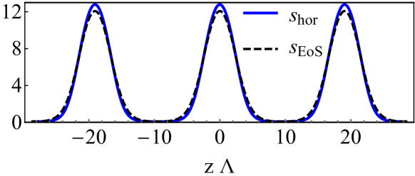
Figure 4: Final entropy density extracted from the area of the horizon (continuous, blue curve) and estimated from the equation of state (dashed, black curve), in units of $\Lambda^{3}/100$.

In the paragraphs above we have been careful to use the term “stationary” as opposed to “static” to refer to the final, time-independent state to which the system settles down. The reason is that the final metric is stationary but not static. The physical reason for this is that the $dtdz$ off-diagonal terms in the final metric do not vanish. As a consequence, the final state is time-independent but not time-reversal invariant (although it is invariant under the simultaneous sign reversal of both $t$ and $z$). The fact that this is a true property of the solution and not just a consequence of our metric ansatz follows from the fact that the timelike Killing vector of our solution is not hypersurface-orthogonal. Interestingly, the $g_{tz}$ component of the final-state metric falls off quickly enough near the AdS boundary so that there is no energy flux in the $z$-direction. In other words, the one-point function of the $T^{t}_{z}$ component of the boundary stress tensor vanishes identically. As a consequence, at the level of one-point functions the final state on the gauge theory side looks not only stationary but static. Since hydrodynamics is an effective theory for one-point functions, in the next section we will speak of a (hydro)static final state. However, it must be kept in mind that the full microscopic state in the gauge theory is only stationary, since $n$-point functions with $n>1$ would be sensitive to the properties of the dual metric deep in the bulk and hence would reveal the lack of staticity.

IV Hydrostatic final state

Previous holographic studies have established that hydrodynamics can describe the evolution of the stress tensor in the presence of large gradients. Here we investigate whether it can also describe the static inhomogeneous configuration at the endpoint of the spinodal instability.

In the hydrodynamic approximation the stress tensor is expanded in spatial gradients in the local fluid rest frame. Up to second order, the constitutive relations are

$$T^{\rm hyd}_{\mu\nu}=T^{\rm ideal}_{\mu\nu}-\eta\,\sigma_{\mu\nu}-\zeta\,\Pi\,\Delta_{\mu\nu}+\Pi_{\mu\nu}^{(2)}$$ (4)

where, in the fluid rest frame, $T_{\mu\nu}^{\rm{ideal}}={\rm Diag}\{{\mathcal{E}},{{P}}_{\rm eq}({\mathcal{E}})\}$, ${{P}}_{\rm eq}({\mathcal{E}})$ is the equilibrium pressure of the homogeneous states shown in Fig. 1, $\sigma_{\mu\nu}$ and $\Pi$ are the shear and bulk stresses, and $\Delta_{\mu\nu}$ is the projector onto the spatial directions. The tensor $\Pi_{\mu\nu}^{(2)}$ contains all the second-order terms. In a non-conformal theory this tensor contains thirteen ${\mathcal{E}}$-dependent second-order transport coefficients and its explicit expression may be found in Romatschke:2009kr . A subset of these coefficients for the model of Attems:2016ugt has been computed in Kleinert:2016nav .

In a static configuration the fluid three-velocity field is identically zero, the stress tensor is diagonal, both $\sigma_{\mu\nu}$ and $\Pi$ vanish, and the leading gradient corrections are those in $\Pi_{\mu\nu}^{(2)}$. This tensor also simplifies since only two independent second-order terms survive in this limit. In the Landau frame, the constitutive relations reduce to

$${{P}}_{L}^{\rm hyd} = {{P}}_{\rm eq}({\mathcal{E}})+c_{\rm L}({\mathcal{E}})(\partial_{z}{\mathcal{E}})^{2}+f_{\rm L}({\mathcal{E}})(\partial^{2}_{z}{\mathcal{E}})\,,$$ (5)

$${{P}}_{T}^{\rm hyd} = {{P}}_{\rm eq}({\mathcal{E}})+c_{\rm T}({\mathcal{E}})(\partial_{z}{\mathcal{E}})^{2}+f_{\rm T}({\mathcal{E}})(\partial^{2}_{z}{\mathcal{E}})\,.$$ (6)

The statement that hydrodynamics describes the final states is the statement that the corresponding pressures are given by these equations with second-order transport coefficients $c_{\rm L,\,T}({\mathcal{E}})$ and $f_{\rm L,\,T}({\mathcal{E}})$ that depend on the local energy density but not on any other details of the final states. We have verified this state independence by varying both the average energy densities within the range shown in Fig. 1 and the length of the circle $L$.

Equivalently, a hydrodynamic description of the final states means that, once $c_{\rm L,\,T}({\mathcal{E}})$ and $f_{\rm L,\,T}({\mathcal{E}})$ have been extracted from a given state (or computed microscopically), they can be used to predict the pressures of a different state given its energy density profile. This is illustrated in Fig. 5, where we compare the true pressures obtained from the gravity side for the end state of Fig. 2 with the hydrodynamic predictions (5) and (6) based on coefficients extracted from a different state. It is remarkable that hydrodynamics works despite the fact that the second-order terms in these equations are as large as the equilibrium pressure, as can be seen in the figure from the difference between the continuous gray curve and the true pressures. This is particularly dramatic for the longitudinal pressure, ${{P}}_{L}$, which must be $z$-independent since, in a static state, conservation of the stress tensor reduces to $\partial_{z}T^{zz}=0$. While the equilibrium contribution to ${{P}}_{L}$ inherits $z$ dependence from the energy density, this modulation is precisely compensated by the second-order contribution. We conclude that the second-order gradients sustain the inhomogeneous state.

Figure 5: (Top) Pressures of the end state of Fig. 2. The true pressures deviate significantly from the ${{P}}_{\rm eq}$ but are in excellent agreement with the hydrodynamic predictions (5)-(6). (Bottom) Zoom-in plot of ${{P}}_{L}$ and difference between the true pressures and the hydrodynamic predictions. Note the different scales in the top and bottom plots.

Taking the applicability of hydrodynamics one step further, we can use it to predict all other static, inhomogeneous configurations. Time independence implies that $P_{L}$ must be constant, which in the hydrodynamic approximation reduces to a second-order, non-linear differential equation for ${\mathcal{E}}(z)$ via Eq. (5). This depends on two integration constants that can be traded for the length of the circle (more precisely, the size of the domains) and the average energy density. Once ${\mathcal{E}}(z)$ is known $P_{T}$ is predicted by Eq. (6).

V Hydrodynamic evolution

The second-order coefficients that we have extracted also control the dynamical evolution of the instability. However, unlike in the stationary final configuration, during the dynamical evolution there are non-zero momentum fluxes, leading to a small but non-vanishing three-velocity field. To approximate the full time evolution by hydrodynamics it is thus necessary to include the first-order shear and bulk tensor contributions in Eq. (4). Similarly, while the systems evolves there are additional second-order gradients beyond those considered in Eqs. (5) and (6). However, these additional second-order terms are quadratic in the velocity field and can be consistently neglected.

In Fig. 6 we show the time evolution of the pressures at $z\,\Lambda=0$. The very early time behavior is the exponential decay of the quasi-normal modes (QNM) that are excited by the perturbation that we introduce to trigger the instability. After this short time, the predictions of second-order hydrodynamics match the true pressures. Second-order terms become increasingly important as the instability saturates, where the first-order approximation, let alone the equilibrium pressure, fails to predict the true pressures while the second-order approximation continues to do so accurately. We conclude that hydrodynamics with large second-order gradients describes the evolution and the saturation of the spinodal instability.

Figure 6: Time evolution of the pressures at $\Lambda z=0$, in units of $\Lambda^{4}/10^{4}$. $P^{\rm{hyd}(1)}$ denotes the hydrodynamic pressure with only first-order terms included, whereas $P^{\rm{hyd}}$ includes these plus the second-order terms of Eqs. (5) and Eq. (6).

VI Discussion

We have uncovered a new example of the applicability of hydrodynamics to systems with large gradients. As in other known examples, part of the reason behind this success is the relaxation of the non-hydrodynamic QNMs at the relevant time scales of the evolution, as in the early transient behaviour observed in Fig. 6. The analysis of the exponential decay of these modes reveals that this process occurs over a time $\Gamma_{\rm QNM}\sim c\,\pi T$ with $c\simeq 3.4$, consistent with Buchel:2015saa . In contrast, for the unstable hydrodynamic mode, assuming $\zeta/\eta\sim 1$ and $\eta/s=1/4\pi$, Eq. (3) yields the typical growth rate $\Gamma\sim\left|c_{s}\right|^{2}\pi T$, which in our case is suppressed with respect to $\Gamma_{\rm QNM}$ by the small value of $\left|c_{s}\right|^{2}\simeq 0.03$. Although this argument may explain why hydrodynamics provides a good description at intermediate times, once the QNMs have decayed, it remains surprising that it also describes the late-time evolution and the final state, where the spatial gradients are large. Moreover, it suggests that it would be interesting to explore other values of the parameter $\phi_{M}$ for which the first-order transition becomes stronger and $\left|c_{s}\right|$ can become of order unity.

Our static inhomogeneous configurations do not describe the separation of the system into two stable phases. For example, the maxima of the end state of Fig. 2 do not lie on the green stable branch but on the red unstable branch of Fig. 1. Presumably the reason is that, if the available average energy density is small, the cost of the necessary gradients for the peaks to reach the green stable branch makes the corresponding configuration disfavored. Similar considerations seem to be responsible for the fact that the final state of Fig. 2 exhibits three identical domains. We have found another static configuration with five peaks which is also well described by hydrodynamics but whose entropy is smaller than that of the three-peak state. Moreover, we have studied the dynamics of the system when perturbed by an $n=1$ mode instead of by an $n=3$ mode. Despite the fact that we have followed the evolution for very long times we have found that this configuration does not seem to settle down to a stationary state; nevertheless, we have observed that throughout its non-linear evolution it develops a second peak. This suggest that a phase separated configuration that naively one would expect to reach by starting with the $n=1$ mode may simply not exist for the average energy density and the box size that we have considered. A logical possibility compatible with all the above is therefore that, under these conditions, the three-peak configuration that we have presented is the thermodynamically preferred state. We emphasize, however, that establishing this definitively would require comparing the entropies of all possible inhomogeneous states of the system with the same average energy density and box size, which is certainly beyond the scope of this paper.

We suspect that the reason why the phase-separated configuration is seemingly not allowed for the box size that we have considered is the fact that the two stable phases in our phase diagram in Fig. 1 differ by several orders of magnitude. This suggests that, in order to realise the phase-separated configuration, one may need a much larger box.

As pointed out above, from the gravity viewpoint the gauge theory spinodal instability translates into an instability of the dual black brane. This is similar to the Gregory-Laflamme instability of a black string in five-dimensional flat space Gregory:1993vy in that it is a long wavelength instability associated to the sound mode of the system that appears below a certain mass or energy density. However, there is also one crucial dissimilarity that makes the time evolution and the final state of our system and those of a black string Lehner:2010pn completely different. This is the fact that the black string is unstable for any mass density below a certain critical value, whereas in our case the black brane is only unstable in a certain energy band (the red dashed curve in Fig. 1). In the case of the black string, at intermediate stages in the evolution the horizon can be described as a sequence of three-dimensional spherical black holes joined by black string segments. Since these segments are themselves subject to a Gregory-Laflamme instability, the evolution results in a self-similar cascade, where ever-smaller satellite black holes form connected by ever-thinner string segments. In contrast, in our case this evolution stops (roughly speaking) once the energy density at a certain point is low enough to lie in the stable region of the phase diagram, i.e. below the dashed red curve in Fig. 1.

- (1) K. H. Ackermann et al. [STAR Collaboration], “Elliptic flow in Au + Au collisions at (S(NN))**(1/2) = 130 GeV,” Phys. Rev. Lett. 86, 402 (2001) [nucl-ex/0009011].
- (2) S. S. Adler et al. [PHENIX Collaboration], “Elliptic flow of identified hadrons in Au+Au collisions at s(NN)**(1/2) = 200-GeV,” Phys. Rev. Lett. 91, 182301 (2003) [nucl-ex/0305013].
- (3) B. B. Back et al. [PHOBOS Collaboration], “Centrality and pseudorapidity dependence of elliptic flow for charged hadrons in Au+Au collisions at s(NN)**(1/2) = 200-GeV,” Phys. Rev. C 72, 051901 (2005) [nucl-ex/0407012].
- (4) G. Aad et al. [ATLAS Collaboration], “Measurement of the azimuthal anisotropy for charged particle production in TeV lead-lead collisions with the ATLAS detector,” Phys. Rev. C 86, 014907 (2012) [arXiv:1203.3087 [hep-ex]].
- (5) S. Chatrchyan et al. [CMS Collaboration], “Measurement of the elliptic anisotropy of charged particles produced in PbPb collisions at =2.76 TeV,” Phys. Rev. C 87, no. 1, 014902 (2013) [arXiv:1204.1409 [nucl-ex]].
- (6) K. Aamodt et al. [ALICE Collaboration], “Elliptic flow of charged particles in Pb-Pb collisions at 2.76 TeV,” Phys. Rev. Lett. 105, 252302 (2010) [arXiv:1011.3914 [nucl-ex]].
- (7) P. Huovinen, P. F. Kolb, U. W. Heinz, P. V. Ruuskanen and S. A. Voloshin, Phys. Lett. B 503, 58 (2001) [hep-ph/0101136].
- (8) D. Teaney, J. Lauret and E. V. Shuryak, nucl-th/0110037.
- (9) T. Hirano, U. W. Heinz, D. Kharzeev, R. Lacey and Y. Nara, Phys. Lett. B 636, 299 (2006) [nucl-th/0511046].
- (10) M. Luzum and P. Romatschke, Phys. Rev. C 78, 034915 (2008); Erratum: [Phys. Rev. C 79, 039903 (2009)] [arXiv:0804.4015 [nucl-th]].
- (11) B. Schenke, S. Jeon and C. Gale, Phys. Rev. Lett. 106, 042301 (2011) [arXiv:1009.3244 [hep-ph]].
- (12) T. Hirano, P. Huovinen and Y. Nara, Phys. Rev. C 84, 011901 (2011) [arXiv:1012.3955 [nucl-th]].
- (13) C. Shen, Z. Qiu, H. Song, J. Bernhard, S. Bass and U. Heinz, arXiv:1409.8164 [nucl-th].
- (14) J. E. Bernhard, J. S. Moreland, S. A. Bass, J. Liu and U. Heinz, arXiv:1605.03954 [nucl-th].
- (15) P. Romatschke, “Do nuclear collisions create a locally equilibrated quark-gluon plasma?,” Eur. Phys. J. C 77, no. 1, 21 (2017) [arXiv:1609.02820 [nucl-th]].
- (16) V. Khachatryan et al. [CMS Collaboration], JHEP 1009, 091 (2010) [arXiv:1009.4122 [hep-ex]].
- (17) G. Aad et al. [ATLAS Collaboration], arXiv:1509.04776 [hep-ex].
- (18) V. Khachatryan et al. [CMS Collaboration], “Evidence for collectivity in collisions at the LHC,” arXiv:1606.06198 [nucl-ex].
- (19) P. Bozek, “Collective flow in p-Pb and d-Pd collisions at TeV energies,” Phys. Rev. C 85, 014911 (2012) [arXiv:1112.0915 [hep-ph]].
- (20) B. Schenke and R. Venugopalan, “Eccentric protons? Sensitivity of flow to system size and shape in p+p, p+Pb and Pb+Pb collisions,” Phys. Rev. Lett. 113, 102301 (2014) [arXiv:1405.3605 [nucl-th]].
- (21) I. Kozlov, M. Luzum, G. Denicol, S. Jeon and C. Gale, “Transverse momentum structure of pair correlations as a signature of collective behavior in small collision systems,” arXiv:1405.3976 [nucl-th].
- (22) R. D. Weller and P. Romatschke, “One fluid to rule them all: viscous hydrodynamic description of event-by-event central p+p, p+Pb and Pb+Pb collisions at TeV,” arXiv:1701.07145 [nucl-th].
- (23) P. M. Chesler and L. G. Yaffe, “Holography and colliding gravitational shock waves in asymptotically AdS5 spacetime,” Phys. Rev. Lett. 106, 021601 (2011) [arXiv:1011.3562 [hep-th]].
- (24) M. P. Heller, R. A. Janik and P. Witaszczyk, “The characteristics of thermalization of boost-invariant plasma from holography,” Phys. Rev. Lett. 108, 201602 (2012) [arXiv:1103.3452 [hep-th]].
- (25) J. Casalderrey-Solana, M. P. Heller, D. Mateos and W. van der Schee, “From full stopping to transparency in a holographic model of heavy ion collisions,” Phys. Rev. Lett. 111, 181601 (2013) [arXiv:1305.4919 [hep-th]].
- (26) P. M. Chesler, “How big are the smallest drops of quark-gluon plasma?,” JHEP 1603, 146 (2016) [arXiv:1601.01583 [hep-th]].
- (27) M. Attems, J. Casalderrey-Solana, D. Mateos, D. Santos-Oliván, C. F. Sopuerta, M. Triana and M. Zilhão, “Holographic collisions in non-conformal theories,” JHEP 1701, 026 (2017) [arXiv:1604.06439 [hep-th]].
- (28) A. Kurkela and Y. Zhu, “Isotropization and hydrodynamization in weakly coupled heavy-ion collisions,” Phys. Rev. Lett. 115 (2015) no.18, 182301 [arXiv:1506.06647 [hep-ph]].
- (29) L. Keegan, A. Kurkela, A. Mazeliauskas and D. Teaney, “Initial conditions for hydrodynamics from weakly coupled pre-equilibrium evolution,” JHEP 1608, 171 (2016) [arXiv:1605.04287 [hep-ph]].
- (30) R. Gregory and R. Laflamme, “Black strings and p-branes are unstable,” Phys. Rev. Lett. 70, 2837 (1993) [hep-th/9301052].
- (31) R. A. Janik, J. Jankowski and H. Soltanpanahi, “Nonequilibrium Dynamics and Phase Transitions in Holographic Models,” Phys. Rev. Lett. 117, no. 9, 091603 (2016) [arXiv:1512.06871 [hep-th]].
- (32) U. Gürsoy, A. Jansen and W. van der Schee, “New dynamical instability in asymptotically anti-de Sitter spacetime,” Phys. Rev. D 94, no. 6, 061901 (2016) [arXiv:1603.07724 [hep-th]].
- (33) O. J. C. Dias, J. E. Santos and B. Way, “Localised and nonuniform thermal states of super-Yang-Mills on a circle,” arXiv:1702.07718 [hep-th].
- (34) M. Attems, J. Casalderrey-Solana, D. Mateos, I. Papadimitriou, D. Santos-Oliván, C. F. Sopuerta, M. Triana and M. Zilhão, “Thermodynamics, transport and relaxation in non-conformal theories,” JHEP 1610, 155 (2016) [arXiv:1603.01254 [hep-th]].
- (35) P. Chomaz, M. Colonna and J. Randrup, “Nuclear spinodal fragmentation,” Phys. Rept. 389, 263 (2004).
- (36) P. Kovtun, D. T. Son and A. O. Starinets, “Viscosity in strongly interacting quantum field theories from black hole physics,” Phys. Rev. Lett. 94, 111601 (2005) [hep-th/0405231].
- (37) C. Eling and Y. Oz, “A Novel Formula for Bulk Viscosity from the Null Horizon Focusing Equation,” JHEP 1106, 007 (2011) [arXiv:1103.1657 [hep-th]].
- (38) M. Attems, J. Casalderrey-Solana, D. Mateos, D. Santos-Oliván, C. F. Sopuerta, M. Triana and M. Zilhão, “Paths to equilibrium in non-conformal collisions,” JHEP 1706, 154 (2017) [arXiv:1703.09681 [hep-th]].
- (39) A. Buchel, “A Holographic perspective on Gubser-Mitra conjecture,” Nucl. Phys. B 731, 109 (2005) [hep-th/0507275].
- (40) R. Emparan, T. Harmark, V. Niarchos and N. A. Obers, “World-Volume Effective Theory for Higher-Dimensional Black Holes,” Phys. Rev. Lett. 102, 191301 (2009) [arXiv:0902.0427 [hep-th]].
- (41) R. Emparan, T. Harmark, V. Niarchos and N. A. Obers, “Essentials of Blackfold Dynamics,” JHEP 1003, 063 (2010) [arXiv:0910.1601 [hep-th]].
- (42) P. Romatschke, “Relativistic Viscous Fluid Dynamics and Non-Equilibrium Entropy,” Class. Quant. Grav. 27, 025006 (2010) [arXiv:0906.4787 [hep-th]].
- (43) P. Kleinert and J. Probst, “Second-Order Hydrodynamics and Universality in Non-Conformal Holographic Fluids,” JHEP 1612, 091 (2016) [arXiv:1610.01081 [hep-th]].
- (44) A. Buchel, M. P. Heller and R. C. Myers, “Equilibration rates in a strongly coupled nonconformal quark-gluon plasma,” Phys. Rev. Lett. 114, no. 25, 251601 (2015) [arXiv:1503.07114 [hep-th]].
- (45) L. Lehner and F. Pretorius, “Black Strings, Low Viscosity Fluids, and Violation of Cosmic Censorship,” Phys. Rev. Lett. 105, 101102 (2010) [arXiv:1006.5960 [hep-th]].