The origin of dust polarization in molecular outflows

Abstract

Aims. Polarization measurements of dust grains aligned with the magnetic field direction are a established technique to trace large-scale field structures. In this paper we present a case study to investigate conditions necessary to detect a characteristic magnetic field substructure embedded in such a large-scale field. A helical magnetic field with a surrounding hourglass shaped field is expected from theoretical predictions and self-consistent magnetohydrodynamical (MHD) simulations to be present in the specific case of protostellar outflows. Hence, such a outflow environment is the perfect environment for our study.

Methods. We present synthetic polarisation maps in the infrared and millimeter regime of simulations of protostellar outflows performed with the newly developed radiative transfer and polarisation code POLARIS. The code, as the first, includes a self-consistent description of various alignement mechanism like the imperfect Davis-Greenstein (IDG) and the radiative torque (RAT) alignment. We investigate for which effects the grain size distribution, inclination, and applied alignement mechanism have.

Results. We find that the IDG mechanism cannot produce any measurable polarization degree ($\geq 1\ \%$) whereas RAT alignment produced polarization degrees of a few $1\ \%$. Furthermore, we developed a method to identify the origin of the polarization. We show that the helical magnetic field in the outflow can only be observed close to the outflow axis and at its tip, whereas in the surrounding regions the hourglass field in the foreground dominates the polarization. Furthermore, the polarization degree in the outflow lobe is lower than in the surroundings in agreement with observations. We also find that the orientation of the polarization vector flips around a few $100\ \rm{\mu m}$ due to the transition from dichroic extinction to thermal re-emission. Hence, in order to avoid ambiguities when interpreting polarization data, we suggest to observed in the far-infrared and mm regime. The actual grain size distribution has only little effect on the emerging polarization maps. Finally, we show that with ALMA it is possible to observe the polarized radiation emerging from protostellar outflows.

1 Introduction

Magnetic fields are responsible for protosteller outflows one of the most prominent signs of star-formation (Pudritz & Norman 1983). Such outflows are more easily to detect than the embedded protostellar disks, from where they are expected to be launched. Hence, the observation of an outflow is a strong indicator for the presence of a rotating disk. Moreover, the launching mechanism of the outflow is closely linked to the disk rotation since the magnetic field lines are frozen at the disk scale and dragged along the direction of rotation. The magnetic field morphology in this scenario is expected to have a strong toroidal component (e.g. Blandford & Payne 1982; Pudritz & Norman 1983; Shibata & Uchida 1985; Tomisaka 1998; Banerjee et al. 2006) forming a helical field morphology together with the large-scale poloidal field of the surrounding medium. Hence, a detection of a helical field component in an outflow would be an additional indicator for the presence of a rotating disk embedded in the center.
From an observational point of view it needs to be verified by proper modeling if the helical field morphological would actually be detectable in the interior of outflow lobes or whether the surrounding hourglass-field dominates light polarization. While recent observations of CO polarization measurements seem to confirm the hypothesis of a helical field (Ching et al. 2016), the interpretation of such data remains still unclear since the magnetic field morphology in the ambient environment represents a possible source of ambiguity. The large-scale magnetic field is expected to be hourglass shaped and is therefore orientated perpendicular to the toroidal component along the line-of-sight (LOS) hiding the embedded helical field morphology (e.g. Girart et al. 2006, 2009).
Focusing on the aspect of the magnetic morphology this can be probed by dust polarization measurements. Historically, the alignment of non-spherical dust grains has long been suggested as a explanation for the observed polarization of stellar radiation (Hiltner 1949; Hall 1949; Martin 1971).
Different theories of grain alignment agree that rotating non-spherical dust grains tend to align with the magnetic field direction (see Lazarian 2007). Unpolarized light will gain polarization by dichroic extinction in the mid-infrared (mid-IR) and thermal dust re-emission from far-infrared (far-IR) to sub-millimeter (sub-mm) and millimeter (mm) wavelength (e.g. Frau et al. 2011) making it possible to infer the projected magnetic field morphology. Hence, polarization measurements provide a promising tool to determine the morphology and subsequently to investigate of the role of magnetic fields in the evolution (Hildebrand et al. 2000; Crutcher 2004; Girart et al. 2012) of star-forming systems. The difficulty is that the reliability of polarization measurements and their interpretation depends on a wide range of physical parameters that are still discussed (see Andersson et al. 2015, for review).
With the dedicated instruments such as the Atacama Large Millimeter Array (ALMA, Brown et al. 2004), and the high-resolution Airborne Wideband Camera-plus instrument of the airborne Stratospheric Observatory For Infrared Astronomy (HAWC+/SOFIA, Dowell et al. 2013), the measurement of dust polarization of cloud cores and disks potentially becomes feasible. Hence, questions about the potential of multi-wavelength polarization measurements to identify specific components of larger structures with complex magnetic field morphology.
Indeed, there are already a number of observations measuring the magnetic field of molecular outflows and the magnetic field in the center of molecular cloud cores. The results, however, seem to contradict each other. Whereas Davidson et al. (2011) and Chapman et al. (2013) report magnetic fields which are preferentially aligned with outflows, Hull et al. (2013, 2014) find magnetic fields to be strongly misaligned with respect to the outflow axis. Hence, simulations of synthetic observations are essential to asses to what accuracy the structure of magnetic fields in star forming cores can be inferred from actual observations. Even for a well-defined field structure as present in Reissl et al. (2014) the resulting polarization pattern is extremely complex and thus not easy to interpret. This holds even more in case that turbulent motions are involved. Hence, we argue that possible conclusions drawn from such observations have to be considered with great care.
The problems tied to the correct interpretation of dust polarization observations that need to be addressed are:

• The measured polarization will naturally only be a projection of the underlying magnetic field morphology since it is averaged along a particular LOS. The question remains to what extend - if at all - the 3D structure of the underlying magnetic field can be deduced by dust polarization measurements.

• It is not clear a priori whether the polarization is observed in dichroic extinction or re-emission since both competing mechanisms are at work simultaneously. This ambiguity whether the projected magnetic field is perpendicular or parallel to the measured polarization vector is often neglected in the literature.

• The observed degree of polarization strongly depends on the composition and size of the dust grains. Hence, uncertainties emerge from unconstrained dust properties, in particular in dense star forming regions.

• There are different theories which can account for the alignment of dust grains under certain conditions. Each dust alignment theory comes with its characteristic polarization pattern making the analysis of polarization measurements highly dependent on the choice of the considered theory.

In order to claim a correlation between the observed orientation of linear polarization and a particular magnetic field structure, it requires careful RT modeling to ensure that the observed wavelengths are actually suitable to probe the regions of interest with aligned dust grains in the first place. However, for RT simulation modeling dust polarization maps often just the density weighted-magnetic field is added up along the LOS (e.g. Soler et al. 2013) or the degree of polarization is adjusted to match observational data (Padovani et al. 2012). Thus, these attempts are of limited predictive capability since they oversimplify the complex physics of radiation-dust interaction and dust grain alignment physics.
For this reason it is required to perform fully self-consistent radiative transfer simulations on linear polarization of radiation incorporating dust grain composition and a well-motivated grain alignment efficiency. In order to do so, we make use of the newly developed 3D RT code POLARIS (Reissl et al. 2016), the only code that is currently available capable of polarization calculations on non-spherical partially aligned dust grains. We study the polarization of mid-IR to mm radiation due to aligned dust grains. Here, we will present a first analysis of synthetic polarization observations obtained from a post-processed MHD simulation (see Seifried et al. 2011, 2012). The simulation models the self-consistent formation of a protostellar disk and its associated molecular outflow driven in the Class 0 stage.
The structure of the paper is as follows: First, we present the properties of the chosen MHD simulation in Sect. 2. We then show details of the applied dust model in Sect. 3. In Sect. 4 the considered theories of dust grain alignment are introduced followed by the description of the RT techniques in Sect. 5. We show the synthetic intensity and polarization maps as a function of different RT simulation parameters in Sect. 6. In Sect. 7 we present a method to determine the origin of polarization by means of tracing distinct rays in RT calculations. We deal with the influence of dust grain size on polarization in Sect. 8 and simulate actual $ALMA$ polarization observations in Sect. 9. Finally, we discuss and summarize the results in Sects. 10 and 11, respectively.

2 MHD - Outflow Simulation

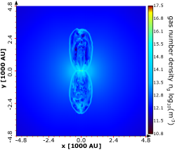
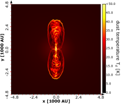
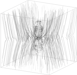
Figure 1: Left panel: Gas number density $n_{\rm{g}}$ of the considered MHD simulation in the mid-plane parallel to the symmetry axis of the outflow lobes. Middle panel: Corresponding dust temperature $T_{\rm{g}}$. The dust temperature was post-processed to account for the stellar contribution of the protostars to dust heating (see Sect. 4 for details). Right panel: 3D magnetic field distribution. The characteristic helical component is in the interior of the outflow lobes embedded within a large scale hourglass shaped field. The box has an edge lengths of $9200\ \rm{AU}$.

The MHD simulation considered in this paper results in the formation of protostars, their surrounding disk, and the protostaller outflow following the collapse of the parental protostellar core. These simulations are performed with the astrophysical code FLASH (Fryxell et al. 2000) using a robust MHD solver developed by Bouchut et al. (2007). To follow the long-term evolution of the protostellar disk and its associated outflow we make use of sink particles (Federrath et al. 2010). For more details on the numerical methods applied we refer the reader to Seifried et al. (2011, 2012).
In this paper we analyze the results of a particular simulation considering the collapse of a 100 $M_{\sun}$ molecular cloud core without initial turbulence, which is $0.25\ \rm{pc}$ in diameter and initially rotating rigidly around the $z$-axis with a rotation frequency of $3.16\cdot 10^{-13}$ s^-1. The ratio of rotational to gravitational energy is $\beta_{\mathrm{rot}}=4\cdot 10^{-2}$. The magnetic field is initially aligned with the rotation axis, i.e. parallel to the $z$-axis and has a strength chosen such that the normalized mass-to-flux ratio is (Spitzer 1978)

$$\mu=\left(\frac{M_{\textrm{core}}}{\Phi_{\textrm{core}}}\right)/\left(\frac{M}{\Phi}\right)_{\textrm{crit}}=\left(\frac{M_{\textrm{core}}}{\int B_{z}\mathrm{d}A}\right)/\left(\frac{0.13}{\sqrt{G}}\right)=26\,.$$ (1)

This corresponds to a initial central magnetic field strength of $132\ \rm{\mu G}$. Hence, the core is magnetically super-critical and the magnetic field can not significantly counteract the initial gravitational collapse of the core. Again, we refer to (Seifried et al. 2011, 2012, - the simulation is called $26-4$ within these papers) for more details on the initial conditions.
During the collapse of the core, a rotationally supported disk builds up around the first protostar. The disk starts to fragment after $\sim 2600\ \rm{yr}$ forming a small cluster of altogether six protostars. A magneto-centrifugally driven protostellar outflow is launched after the formation of the first sink particle, which is well-collimated with a collimation factor of $\sim 4$ by the end of the simulation. The outflow continues expanding in a roughly self-similar fashion keeping the overall morphological properties.
In this work we analyze this outflow at an age of $5000\ \rm{yr}$. By this time the outflow lobe has a height of $3200\ \rm{AU}$ above and below the disk midplane and a maximum outflow speed of about $19\ \rm{km\ s}^{-1}$, which is well above the escape velocity. Note, that this maximal value is attained close to the disk and that most of the gas in the outflow is a few $\rm{km\ s}^{-1}$ slower. The six protostars cover a range of luminosities between $0.22\ L_{\rm{\odot}}$ and $81.4\ L_{\rm{\odot}}$. We model the luminosities taking also the accretion onto the surface of the protostars into account which provides a significant part to the total luminosity in this stage of star formation (see Offner et al. 2009, for details).
The mid-plane gas number density $n_{\rm{g}}$, dust temperature $T_{\rm{d}}$, as well as the 3D magnetic field morphology of the considered snapshot are shown in Fig. 1. Investigating the magnetic field structure within the outflow lobes, we find that the toroidal magnetic field component clearly dominates over the poloidal component while the field outside the outflow lobe is hourglass shaped. Furthermore, we observed the occurrence of several shocks within the outflow locally leading to rather unordered gas motions and magnetic field orientations.

3 Constraints to dust modeling

The interpretation of observational polarization data strongly depends on the parameter of the considered dust grain model. While we know for sure that grains in the interstellar medium (ISM) are not spherically symmetric, their actual shape, composition and size distribution is uncertain.
A satisfactory model, the so called MRN model (Mathis et al. 1977), reproducing the galactic extinction curve, is a three parameter model with a power-law size distribution $n(a)\propto a^{-q}$ and a dust grain size range of $a\in[a_{\rm{min}}:a_{\rm{max}}]$ with values of $q=-3.5$, $a_{\rm{min}}=5\ \rm{nm}$, and $a_{\rm{max}}=250\ \rm{nm}$. In subsequent studies, the upper limit was extended to be of $\rm{\mu m}$ - size (e.g. Clayton et al. 2003; Draine & Li 2007). To account for characteristic extinction and absorption features, an ensemble of dust materials is used consisting of a mixture of carbonaceous (graphite) and silicate (olivene) materials (e.g. Zubko 1995; Zhukovska et al. 2016). Additionally, in the case of IDG alignment we considered ferromagnetic particles encapsulated in the dust grains enhancing paramagnetic alignment by a factor of $10^{2}$ (Jones & Spitzer 1967; Djouadi et al. 2007; Belley et al. 2009). An oblate dust grain with an fixed aspect ratio represents a particularly promising approach for simulating the interstellar polarization and extinction data (Lee & Draine 1985; Kim & Martin 1995; Hildebrand & Dragovan 1995) so, here we use an average value of $0.5$.
Since, the different grain materials have unique dielectric and paramagnetic properties this also results in a unique alignment behavior. Analyzing the linear polarization and circular polarization shows that a higher alignment efficiency is to be expected for silicate grain while carbonaceous grains seem to remain unaffected by the presence of a magnetic field (e.g Martin & Angel 1976; Mathis 1986). Hence, we consider carbonaceous grains to be randomized, while silicate grains are partially aligned in our model (Clayton et al. 2003; Draine & Li 2007).
The dust properties required for the self-consistent dust grain heating calculations and polarization simulations are the efficiencies $Q$ of light polarization parallel ($Q_{\rm{||}}$) and perpendicular ($Q_{\rm{\bot}}$) to the grain symmetry axis (see e.g. Martin 1971). The efficiencies can be pre-calculated by a numerical method representing the dust grains shape as an array of material specific discrete dipoles (Draine & Flatau 2000). In order to remain consistent with the constraints of interstellar dust parameter we used the DDSCAT 7.2 code (see Draine & Flatau 2013) to calculate values of $Q$ for an aspect ratio of $0.5$ in a regime of wavelength $\lambda\in[0.9\ \rm{\mu m}:3\ \rm{mm}]$ and grain sizes limits of $a_{\rm{min}}=5\ \rm{nm}$ and $a_{\rm{max}}=2\ \rm{\mu m}$. Here, the number of dipoles in our calculations ranges from $N=171\,500-296\,352$ to remain in the numerical limit ($a<0.05\lambda\sqrt[3]{N}/|m|$) of the DDSCAT code, where $|m|$ is the complex refractive index. For the input to DDSCAT we use the refractory indices of (Draine & Lee 1984; Laor & Draine 1993; Weingartner & Draine 2000). Dust grain with sizes with radii larger than $a>2\mu m$ are outside the reach of DDSCAT. In order to overcome the numerical limit we combined existing data from DDSCAT with data obtained by the MIEX code (Wolf & Voshchinnikov 2004) using mie-scattering to smoothly extrapolate our dust model up to an upper cut-off radius of $a_{\rm{max}}=200\rm{\mu m}$. We consider the upper radius in our outflow environment to be larger than in the ISM and make the model with $a_{\rm{max}}=2\ \rm{\mu m}$ as our default mode.
The POLARIS RT simulations are performed with the cross-sections for a dust grain of average size with

$$\overline{C}_{\rm{X}}=\sum_{i}{\kappa_{i}\cdot\int_{a_{\rm{min}}}^{a_{\rm{max}}}\pi a^{2}(Q_{\rm{X,i,||}}+Q_{\rm{X,i,\bot}})n(a)R(a)da},$$ (2)

where $\pi a^{2}$ is the geometrical cross-section, $\kappa_{i}$ is the fraction of distinct dust grain materials, and $\overline{C}_{\rm{X}}$ stands for the cross sections of extinction ($C_{\rm{e}}$), absorption ($C_{\rm{a}}$) and scattering ($C_{s}$), respectively. The same averaging is applied for the cross sections $\Delta C_{\rm{e}}$ for dichroic extinction, for thermal re-emission $\Delta C_{\rm{a}}$, and circular polarization $\Delta C_{\rm{c}}$ with

$$\Delta\overline{C}_{\rm{X}}=\sum_{i}{\kappa_{i}\cdot\int_{a_{\rm{min}}}^{a_{\rm{max}}}\pi a^{2}(Q_{\rm{X,i,||}}-Q_{\rm{X,i,\bot}})\sin^{2}(\vartheta)n(a)R(a)da}.$$ (3)

Here, the cross sections are weighted by the Rayleigh reduction factor $R(a)$ (see e.g. Greenberg 1968; Lazarian 2007, for details), to account for imperfect grain alignment. $R(a)=1$ corresponds to perfect alignment along the direction of the magnetic field and $R(a)=0$ to randomly orientated dust grains, respectively. The angle $\vartheta$ is defined by the direction of the incident light and the magnetic field direction. Consequently, no linear polarization emerges along a LOS parallel to the magnetic field direction since the dust grain would appear to be spherical (see Reissl et al. 2014, for details).

4 Dust grain alignment

The alignment of the rotation axis of a dust grain parallel to the direction of the magnetic field lines is due to paramagnetic effects within the grain material itself (e.g. Davis & Greenstein 1951; Barnett 1917). However, in the ISM perfect alignment is suppressed by gas-dust collisions and the interaction with the local radiation field.
Here, we go beyond previous approaches in this field (e.g. Kim & Martin 1995; Draine & Fraisse 2009; Padovani et al. 2012) and include the the classical imperfect Davis-Greenstein (IDG) alignment due to paramagnetic relaxation (Davis & Greenstein 1951; Jones & Spitzer 1967; Purcell 1979) with as well as the radiative torque alignment (RAT) due to radiation-dust interaction (Dolginov & Mitrofanov 1976; Draine & Weingartner 1996, 1997; Hoang & Lazarian 2007a, 2009) in the MC RT simulations. Additionally, we consider the randomization of dust grains caused by thermal fluctuations in the dust grain material for the grain alignment efficiency (see Lazarian & Roberge 1997).
The IDG alignment is mainly determined by the parameter

$$\delta_{\textit{0}}=2.07\cdot 10^{20}\frac{\textbf{B}^{2}}{n_{\textit{g}}T_{\textit{d}}\sqrt{T_{\textit{g}}}},$$ (4)

that represents an upper threshold for the dust grain alignment. The IDG accounts for the alignment of small dust grains because grains with an effective radius above $\delta_{\textit{0}}$ do no longer significantly contribute to the net polarization (see Jones & Spitzer 1967, for details). Ferromagnetic inclusions can enhance the grain alignment efficiency by several orders of magnitude (see e.g. Andersson et al. 2015, for review).
Irregular dust grains are expected to scatter left handed and right handed circular light differently (Dolginov & Mitrofanov 1976; Weingartner & Draine 2003). This additional radiative torque (RAT) increases the aliment efficiency (Hoang & Lazarian 2007a, b). The RAT alignment assumes dust grains to align efficiently when the angular velocity $\omega_{\rm{rad}}$ resulting from RATs becomes dominant over the angular velocity $\omega_{\rm{gas}}$ caused by random gas bombardment so that $\omega_{\rm{rad}}\geq 3\times\omega_{\rm{gas}}$. Consequently, RAT alignment is determined by the ratio of angular velocities. The minimum grain radius $a_{\rm{alg}}$ at which dust grains start to align is determined by:

$$\left(\frac{\omega_{\rm{rad}}}{\omega_{\rm{gas}}}\right)^{2}=\frac{a_{\rm{alg}}\rho_{\rm{d}}}{\delta m_{\rm{H}}}\left(\frac{t_{\rm{gas}}}{(t_{\rm{gas}}+t_{\rm{rad}})n_{\rm{g}}k_{B}T_{\rm{g}}}\int Q_{\Gamma}(\epsilon)\lambda\gamma_{\rm{\lambda}}\overline{u}_{\rm{\lambda}}d\lambda\right)^{2}.$$ (5)

Here, $\rho_{\rm{d}}$ is the density of the dust grain material and $\overline{u}_{\rm{\lambda}}$ is the local mean energy density of the radiation field. The wavelength specific anisotropy factor $\gamma_{\rm{\lambda}}$ varies between $\gamma_{\rm{\lambda}}=1$ for unidirectional radiation and $\gamma_{\rm{\lambda}}=0$ for an isotropic radiation field. For details about the constant $\delta$ and the characteristic gas drag time $t_{\rm{gas}}$ and thermal emission drag time $t_{\rm{rad}}$, respectively, we refer to Draine & Weingartner (1997). The radiative torque efficiency depends $Q_{\Gamma}(\epsilon)$ on the angle $\epsilon$ between the predominant direction of radiation and the magnetic field direction and allows to calculate the characteristic dust grain size $a_{\rm{alg}}$ at which dust grains start to align. For further details see Reissl et al. (2016).

5 Radiative transfer calculations

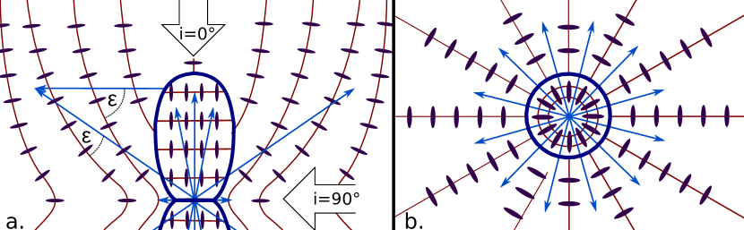
Figure 2: Schematic illustration of the expected dust grain (dark blue ellipses) alignment behavior according to IDG and RAT alignment in the center plane perpendicular (panel a.) and parallel (panel b.) to the symmetry axis of the outflow lobes (blue). The angle $\epsilon$ is defined to be between the predominant direction of the radiation (light blue arrows) and the magnetic field lines (red). The white arrows indicate the definition of the inclination angle.

To create synthetic polarization maps we postprocess the data resulting from the MHD simulations discussed in Sect. 2 in a three step approach. At first, we update the initial MHD dust temperature in a Monte-Carlo (MC) simulation (see Lucy 1999; Bjorkman & Wood 2001; Reissl et al. 2016, for details) using the luminositis and position of the emerged cluster of protostars (see Sect. 2).
Secondly, the anisotropy parameter $\gamma_{\rm{\lambda}}$ as well as the local energy density required by the RAT alignment is calculated in a second MC process. Here, we make again use of the method proposed in Lucy (1999) using the path lengths and direction of all photons crossing a cell to obtain:

$$\textbf{u}_{\rm{\lambda}}d\lambda=\frac{\epsilon_{\rm{0}}}{c\Delta tV_{\rm{cell}}}\sum_{d\lambda}\frac{l\cdot\textbf{k}}{\left|\textbf{k}\right|}.$$ (6)

With that, we can finally calculate the polarization maps. The wavelength regime considered in this paper covers the mid-IR to the far-IR, sub-mm and mm ($\approx 20\ \rm{\mu m}-3000\ \rm{\mu m}$).
A polarization pattern can also emerge because of scattering on dust grains. The quantity that quantifies the influence of scattering to the net polarization is the albedo $\alpha=C_{\rm{sca}}/C_{\rm{ext}}\in[0;1]$ where $\alpha=1$ means that the polarization is completely dominated by scattering and $\alpha=0$ stands for no scattering at all. Indeed, for the considered dust grain models with an upper cut-off radii of $a_{max}=2\ \rm{mm}$ the albedo $\alpha\approx 0.25$ at a wavelength of $\lambda=20\ \rm{\mu m}$. Hence, scattering can influence the polarization pattern especially near the disc region under such conditions. However, we start our investigation with an upper cut of radius of $a_{max}=250\ \rm{nm}$ where $\alpha\approx 0.01$ at $\lambda=20\ \rm{\mu m}$. Larger dust grains are just applied for synthetic polarization maps in the $mm$ regime of wavelength where $\alpha<<10^{-3}$ for all dust models. Hence, we neglect the influence of scattering within the scope of this paper.
The method of choice to represent the resulting polarization are the Stokes parameter $(I,Q,U,V)$. Here, $I$ stands for intensity, $Q$ and $U$ for linear polarization and $V$ for circular polarization. The radiative transfer in the Stokes formalism leads to a set of equations (see Martin 1974, for details) considering the dust grains as black body radiators that can be solved analytically. This allows to calculate the contribution $(I^{\prime},Q^{\prime},U^{\prime},V^{\prime})$ of each cell (see Whitney & Wolff 2002) with the Planck function $B_{\rm{\lambda}}(T_{\rm{d}})$ along each path element $dl$ with

$$I^{\prime}=\left(I+Q\right)e^{-n_{\rm{d}}l\left(C_{\rm{e}}+\Delta C_{\rm{e}}\right)}+n_{\rm{d}}lB_{\rm{\lambda}}(T_{\rm{d}})\left[C_{\rm{a}}+\Delta C_{\rm{a}}\cos(2\phi)\right],$$ (7)

$$Q^{\prime}=\left(I-Q\right)e^{n_{\rm{d}}l\left(\Delta C_{\rm{e}}-C_{\rm{e}}\right)}-n_{\rm{d}}lB_{\rm{\lambda}}(T_{\rm{d}})\left[C_{\rm{a}}+\Delta C_{\rm{a}}\cos(2\phi)\right],$$ (8)

$$U^{\prime}=e^{-n_{\rm{d}}lC_{\rm{e}}}\left[U\cos(n_{\rm{d}}l\Delta C_{\rm{c}})-V\sin(n_{\rm{d}}l\Delta C_{\rm{c}})\right]+n_{\rm{d}}l\Delta C_{\rm{a}}B_{\rm{\lambda}}(T_{\rm{d}})$$ (9)

and

$$V^{\prime}=e^{-n_{\rm{d}}lC_{\rm{e}}}\left[U\sin(n_{\rm{d}}l\Delta C_{\rm{c}})-V\cos(n_{\rm{d}}l\Delta C_{\rm{c}})\right].$$ (10)

Here, $n_{\rm{d}}$ is the number density of the dust. The angle $\phi$ is between the direction of light polarization and the magnetic field lines. Note that because of the $\phi$ dependency circular polarization can only emerge in regions where each following magnetic field line and subsequently the preferential axis of grain alignment is non-parallel to the previous one along the LOS (see e.g. Martin 1974). The hourglass component in the outside region is such a magnetic field with rather parallel field lines along the LOS. As a result of this we get most of the circular polarization from within the outflow lobes in our RT calculations. Here, the maximum of the degree of circular polarization can amount up to $\pm 0.4\ \%$. As shown in Reissl et al. (2014) the pattern of circular polarization provides additional information to distinguish between different well ordered magnetic field morphologies. However, due to the chaotic nature of the helical field the results are inconclusive and do not allow to identify the helical component by any characteristic circular polarization pattern. Hence, we focus only on linear polarization in this paper. However, circular polarization still needs to be considered in the RT calculation because a permanent transfer from circular polarization ($V$ - parameter) to linear polarization ($U$ - parameter) and vise versa occurs.
The degree and orientation of linear polarization $P_{\rm{l}}$ is determined by

$$P_{\rm{l}}=\frac{I_{\rm{p}}}{I}=\frac{\sqrt{Q^{2}+U^{2}}}{I},$$ (11)

where $I_{\rm{p}}$ is the polarized intensity. Its position $\chi_{\rm{Pl}}$ angle on the plane of the sky is defined by

$$\chi_{\rm{Pl}}=\frac{1}{2}\arctan\left(\frac{U}{Q}\right).$$ (12)

For a more detailed description we refer to Reissl et al. (2014, 2016).

6 Synthetic polarization maps

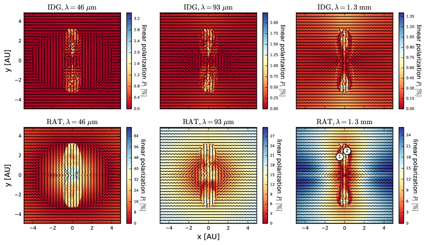
Figure 3: Maps showing the degree of linear polarization $P_{\rm{l}}$ (color coded) overlaid with normalized orientation vectors for the three distinct wavelengths of $\lambda=46\ \rm{\mu m}$ (left column), $\lambda=93\ \rm{\mu m}$ (middle column), and $\lambda=1.3\ \rm{mm}$ (right column), respectively, at an inclination angle of $90^{\circ}$. The top row shows the maps considering IDG alignment while the bottom row shows the results considering RAT alignment. The numbers in the right bottom panel correspond to the LOS shown in Figs. 6 and 6. Note, that only the panels for $\lambda=93\ \rm{\mu m}$ trace the helical magnetic field.

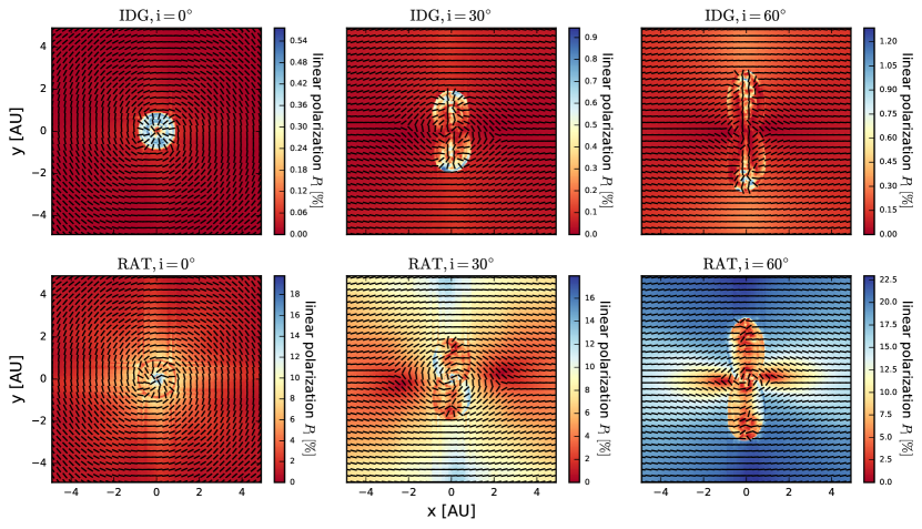
Figure 4: Maps showing the degree of linear polarization $P_{\rm{l}}$ (color coded) overlaid with normalized orientation vectors for a wavelength of $\lambda=1.3\ \rm{mm}$ at the three distinct inclination angles $i=0^{\circ}$ (left column), $i=30^{\circ}$, $i=0^{\circ}$ (middle column), and $i=60^{\circ}$ (right column), respectively. The top row shows the maps considering IDG alignment while the bottom row shows the results considering RAT alignment. Note also that the polarization degree varies strongly strongly between the two alignment theories and for different wavelength.

6.1 Linear polarization by RAT and IDG alignment

In this section we investigate how the polarization pattern depends on grain alignment theory, inclination angle, and wavelength. Here, it is essential to estimate the expected contributions of different grain alignment theories to the net polarization separately. For the physical conditions present in the MHD simulation, both IDG and RAT alignment theory predict a similar behavior with regard to the preferential axis of grain alignment. However, the alignment efficiency and consequently the detectability of a polarization signal may differ significantly for different alignment theories. Furthermore, the two competing polarization mechanisms of dichroic extinction and thermal re-emission contribute both to linear polarization. Dichroic extinction dominates polarization in the UV, optical, and near-IR regime and leads to polarization parallel to the magnetic field direction. In contrast to dichroic extinction, thermal re-emission results in light polarization perpendicular to the magnetic field for a wavelength from the mid-IR to the mm. It is expected that in an intermediate regime of wavelengths both effects cancel each other out and that therefore the polarization vectors flip their orientation by $90^{\circ}$ in the transition. Hence, in order to determine the intermediate regime of wavelengths where dichroic extinction transitions to thermal re-emission we simulated synthetic polarization maps. The maps are calculated with an upper cut-off radius of $a_{\rm{max}}=2\ \rm{\mu m}$ and cover a wavelength regime of $20\ \rm{\mu m}-3\ \rm{mm}$. The disk is seen edge-on.
In Fig. 2 an illustration of the expected grain alignment is shown for a better interpretation of the following polarization maps. For an inclination of $90^{\circ}$ the resulting maps of linear polarization calculated with IDG and RAT alignment theory are shown in Fig. 3. Although the IDG and RAT alignment theories are based on different physical principles, the resulting overall orientation of polarization vectors over wavelength are comparable.However, we note that the degree of linear polarization varies significantly between the two alignment theories with RAT leading to mach larger polarization values.
With increasing wavelength, the contribution of thermal re-emission to polarization becomes increasingly dominant over dichroic extinction. Since both competing polarization effects contribute in directions perpendicular to each other, it is possible that the net polarization vector flips by $90^{\circ}$ or is even canceled out.
The wavelength at which thermal re-emission starts to appear in the polarization maps for both IDG and RAT alignment is at $\lambda\simeq 40\ \rm{\mu m}$. The outer most regions of the polarization maps are less dense than the center and hence less affected by dichroic extinction. Therefore, polarization by thermal re-emission appears first in the outer part of the polarization maps an moves towards the center for longer wavelength. For a wavelength of $\lambda\simeq 46\ \rm{\mu m}$ the outflow lobe is still unaffected by the effect of flipping polarization vectors (Figs. 3 left column). Here, the outer regions of the polarization maps are dominated by thermal re-emission while the center regions are still polarized due to dichroic extinction. In the case of RAT alignment (Figs. 3 left bottom panel) this leads to a characteristic ring-shaped gap with a minimum degree of linear polarization where the contributions of dichroic extinction and thermal re-emission cancel out each other. For the IDG alignment (Figs. 3 left top panel) this effect is less pronounced and hardly detectable because of the overall low degree of linear polarization in that area.The IDG alignment is highly suppressed in high density and temperature regions (see Eq. 4) and would thus allow no conclusion about the underlying magnetic field morphology near the disk region.
At a wavelength of about $\lambda\simeq 93\ \rm{\mu m}$ (see Fig. 3 middle column) the outflow lobes are completely enclosed by the region of thermal re-emission while the polarization in the lobes itself results from dichroic extinction. This is due to the dust temperature of $T_{\rm{d}}\approx 30\ \rm{K}-40\ \rm{K}$ at the surface of the outflow lobes (see Fig. 1 middle panel) corresponding to a pack emission at $\lambda\approx 70\ \rm{\mu m}-97\ \rm{\mu m}$. The outside regions with $T_{\rm{d}}\approx 10\ \rm{K}$ contributes a neglectable amount of radiation at that wavelength regime. Consequently, the dust grains in front of the outflow lobes are illuminated by a strong background radiation emitted by the surface of the outflows and dichroic extinction dominates the polarization.
Going to even longer wavelength for both RAT and IDG, thermal dust re-emission dominates the entire map at $\lambda\simeq 600\ \rm{\mu m}$ resulting to a polarization pattern comparable to that shown in Fig. 3 in the right columns. For larger wavelength on the polarization vectors are perpendicular to the projected magnetic field and their orientation remains rather constant up to the $\rm{mm}$ regime of wavelength.
As shown by detailed analysis (see Sect. 7) even in the inner disk region linear polarization is completely due to thermal remission. Hence, in the maps considering IDG and RAT alignment the orientation of the polarization vectors represent the projected magnetic field morphology. In contrast to RAT alignment the helical component remains slightly more apparent at the tops and near the symmetry axis of the outflow lobes for IDG.

6.2 Impact of inclination angle

So far, we examined the polarization orientation and degree dependence on grain alignment theory and wavelength for a fixed inclination angle of $90^{\circ}$ between the outflow axis and the LOS. However, interpretation of polarization measurements are also influenced by projections effects. In this section we to investigate how the linear polarization pattern changes as a function of the inclination towards the observer. Due to the ambiguities in the mid-IR and sub-mm discussed in Sect. 6.1 and with regards to the simulation of synthetic observations with the $ALMA$ telescope array we focus here on a wavelength of $\lambda=1.3\ \rm{mm}$, where the polarization is purely due to thermal re-emission, i.e. the polarization vector is perpendicular to the field.
Fig. 4 shows polarization maps considering IDG alignment in comparison to RAT alignment for the three different inclination angles $i$ of $0^{\circ}$ (disk is face on), $45^{\circ}$, and $90^{\circ}$, respectively. Again, note that the polarization degree differs by more than one order of magnitude. For IDG alignment and an inclination angle of $i=0^{\circ}$ (Fig. 4 top left panel), the LOS towards the center of the maps is parallel to the hourglass magnetic field (see Fig. 2). Since no linear polarization can occur in the case of a LOS parallel to the magnetic field (see Sect. 3), the linear polarization emerges completely in the interior of the outflow lobes and the disk component. With increasing inclination angle the contributions from the hourglass field start to dominate the overall orientation of linear polarization. For an inclination of $i=45^{\circ}$ (see middle top panel of Figs. 4) the polarization pattern begins to resemble the projected hourglass morphology. The helical component of the magnetic field, however, remains apparent close to the symmetry axis and at the tips of the outflows, e.g. the orientation of the polarization vectors is predominantly vertical.
In the bottom row of Fig. 4 we show the linear polarization maps considering RAT alignment. For an inclination angle of $i=0^{\circ}$ the results are qualitatively the same as the ones for IDG alignment. However, with increasing inclination angle the contributions of the surrounding hourglass shaped magnetic field becomes even earlier dominant than for IDG alignment. Here, just the regions close to tips of the outflow lobes match the helical magnetic field component, i.e. the polarization vectors are vertically orientated.
When the subsequent magnetic field lines cross each other along the LOS, the polarized emissions of a given dust grain is canceled out by the emission of another one leading to an area of reduced linear polarization. This projection effect of crossing field lines along the LOS becomes apparent in the maps with RAT alignment (Fig. 4 bottom row) where two polarization holes (bottom middle panel) and two extra lobes of minimum of linear polarization (bottom right panel), respectively, become visible perpendicular to the symmetry axis of the outflow lobes. Here, these extra lobes are not a result of reduced dust density or temperature fluctuations, but are simply a projection effect and an indicator of the underlying hourglass-shaped field morphology (see also Reissl et al. 2014).
The same effect can be observed for the polarization maps with IDG alignment in the top middle panel and top right panel of Figs. 4. However, the already low degree of linear polarization due to inefficient grain alignment outside the outflow lobes makes these projection effects less relevant.
Despite the additional ferromagnetic inclusions considered for the IDG alignment calculations, the maximum degree of linear polarization is of the order of a few per cent. This makes RAT alignment the relevant alignment process for observations in the presented outflow environment. Hence, recent efforts of Hoang & Lazarian (2016) showed that it is possible to combine IDG and RAT alignment. However, we conclude that IDG is neglectable in the considered outflow environment and focus on RAT alignment alone in the following sections.

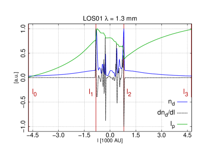
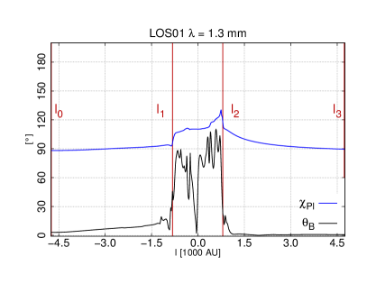
Figure 5: Physical quantities along the a exemplary LOS $\#1$ in the bottom right of Fig. 3. The vertical red lines indicate the borders between the first outer region ($l_{\rm{0}}-l_{\rm{1}}$), the interior of the outflow lobes ($l_{\rm{1}}-l_{\rm{2}}$), and the second outer region ($l_{\rm{2}}-l_{\rm{3}}$), respectively. Left panel: Normalized values of polarized intensity $I_{\rm{p}}$ (green), dust number density $n_{\rm{d}}$ (blue), and its first derivative $dn_{\rm{d}}(l)/dl$ (dotted black). Note, that the polarized intensity $I_{\rm{p}}$ is plotted as a cumulative value. Right panel: Orientation angles of linear polarization $\chi_{\rm{P_{l}}}$ (blue) and magnetic field direction $\theta_{\rm{B}}$ (black). An orientation angle of $0^{\circ}$ corresponds to vertical polarization vectors in all figures shown in this paper.

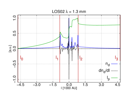
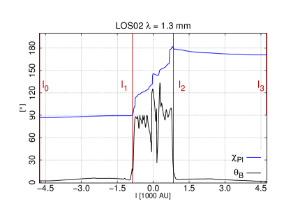
Figure 6: Same as Fig. 6 along the LOS $\#2$ in the bottom right panel of Fig. 3.

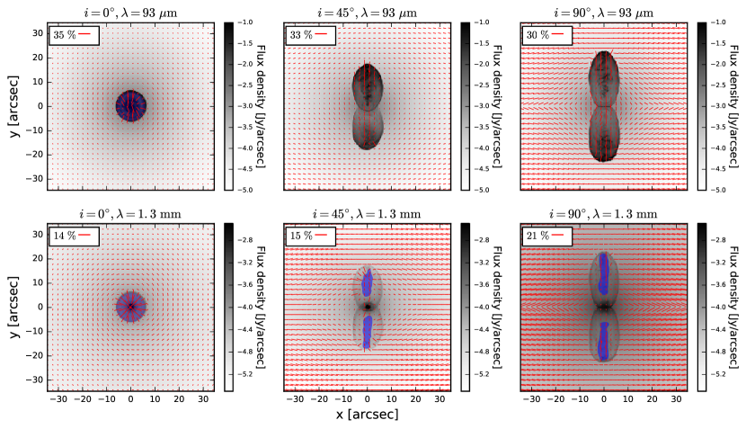
Figure 7: Synthetic flux density maps (grey coded) with a wavelength of $\lambda=93\ \rm{\mu m}$ (top row) and $\lambda=1.3\ \rm{mm}$ (bottom row) and a distance of $140\ \rm{pc}$ overlaid with vectors of linear polarization considering RAT alignment for inclination angles of $i=0^{\circ}$ (left column), $i=45^{\circ}$ (middle column), and $i=90^{\circ}$ (right column) and a maximal dust grain radius of $a_{\rm{max}}=2\ \rm{\mu m}$. The length of the vectors depends on the degree of linear polarization. For better comparison the colorbar is fixed in each row. The blue colored areas indicate where the polarization vectors represent the helical magnetic field structure of the outflow according to LOS analysis.

7 Origin of linear polarization

In the previous sections we discussed maps of linear polarization on the basis of physically well motivated dust grain alignment theories and dust modeling. In these efforts it remained unclear to what extend the outflow lobes and the surrounding medium contribute to the synthetic maps of net polarization. Consequently, the synthetic polarization maps of Figs. 3 and 4 remain still ambiguous regarding the question of what component of the magnetic field is actually traced (hourglass in front of the outflow lobes or in the helical field).
This problem is even more severe for actual observations. Here, the spatial information of density and temperature as well as the magnetic field morphology in any observed astrophysical system gets lost due to the projection along a particular LOS. In contrast to observations, synthetic data by RT calculations allows to trace different LOS through the 3D MHD simulation and subsequently to determine the actual origin of polarization. In the following we focus on the origin and the actual detectability of polarization pattern characteristic for helical and hourglass magnetic field structures. Hence, we implemented an heuristic algorithm to analyze the polarization state of radiation along a distinct LOS $l$.
This automatized heuristic approach works in three steps:

1. Identification of the distinct regions inside and outside the outflow lobes. Here, we detect the bow shock of the outflow lobes by analyzing the first derivative of the gas number density $dn_{\rm{g}}/dl$ (Figs. 6 and 6 left panels in black dotted lines). This allows to distinguish between three regions along the LOS. The first outside region expands from $l_{\rm{0}}$ to $l_{\rm{1}}$, the outflows itself from $l_{\rm{1}}$ to $l_{\rm{2}}$, and the second outside region from $l_{\rm{2}}$ to $l_{\rm{3}}$ (indicated in Figs. 6 and 6 as red vertical lines).

2. Ray-tracing through the MHD simulation data in order to keep track of the accumulated polarized intensity $I_{\rm{p}}$ (Figs. 6 and 6 left panels in green lines), the orientation angle of linear polarization $\chi_{\rm{Pl}}$ (Figs. 6 and 6 right panels in blue lines) and the orientation angle $\theta_{\rm{B}}$ (Figs. 6 and 6 right panels in black lines) of the magnetic field with respect to the symmetry axis of the outflow lobes.

3. Determining origin of polarization by analyzing the largest increase in $I_{\rm{p}}$ as well as the relative orientation between magnetic field lines and linear polarization.

With this simple but effective scheme, the actual origin of linear polarization can be determined. The first criterion is the increase or decrease, respectively, of polarized intensity $I_{\rm{p}}$ along each LOS. Here, it is sufficient to compare the accumulated polarized intensity at the points $I_{p}(l_{\rm{0}})$, $I_{p}(l_{\rm{1}})$, $I_{p}(l_{\rm{2}})$, and $I_{p}(l_{3})$ to determine the area with the largest increase.
The second criterion is the resulting polarization angle with respect to the local magnetic field direction. Although the magnetic field direction in the outflow lobes is not well ordered it appears indeed rather regular in projection and can therefore be assumed to be perpendicular to the projected magnetic field direction in both outside regions.
We assume that the linear polarization originates from the interior of the outflow lobes when the largest increase in polarized intensity is inside the outflow lobe, and the orientation vector of linear polarization deviates from the projected helical field direction by less than $\pm 20^{\circ}$.
Here it needs to be emphasized, that this heuristic method is fine tuned to probe the outflow lobes in just this particular MHD simulation. The parameters of this heuristic approach are optimized by proper testing by minimizing the the false positive results. A manual evaluation of $75$ randomly chosen LOSs for each of the different inclination angles and wavelengths revealed that the accuracy of the correct detection of the origin of linear polarization is larger than $85\ \rm{\%}$. Consequently, the areas in the polarization maps where linear polarization originates from the inside of the outflow lobes can be identified with high precision. However, the number of LOSs probing the helical field might actually be larger because of possible false negative detections.
Figs. 6 and 6 show the resulting plots of two exemplary LOSs corresponding to the positions in the right bottom panel of Fig. 3 at a wavelength of $\lambda=1.3\ \rm{mm}$. In the left panel of Fig. 6 the polarized intensity $I_{\rm{p}}$ emerges in the first outer region ($l_{\rm{0}}-l_{\rm{1}}$) and jumps to a maximum near the edge at $l_{\rm{1}}$ of the outflow lobe, decreases in the interior ($l_{\rm{1}}-l_{\rm{2}}$) with a strong correlation to jumps in dust number density $n_{\rm{d}}$ and reaches its absolute maximum at the border of the grid at position $l_{\rm{3}}$.
In the first outside region ($l_{\rm{0}}-l_{\rm{1}}$) the orientation angle $\chi_{\rm{Pl}}$ (see 12) remains at an almost constant value of roughly $90^{\circ}$ with respect to the magnetic field orientation $\theta_{B}$ and increases slightly near the first edge ($l_{\rm{1}}$) of the outflow lobe as it is shown in the right panel of Fig. 6. In the interior ($l_{\rm{1}}-l_{\rm{2}}$) the polarization angle remains again almost constant and trends back to $90^{\circ}$ as the radiation propagates towards the border ($l_{\rm{3}}$) of the model space. In this case the interior of the outflow lobe is of minor influence to linear polarization with respect to degree and orientation. Clearly, the $LOS01$ does not probe the helical component of the magnetic field morphology but only the hourglass foreground.
Along the second LOS shown in Fig. 6, the polarized intensity $I_{\rm{p}}$ shows the same trend as in Fig. 6 and the orientation angle $\chi_{\rm{Pl}}$ remains at around $90^{\circ}$ up to the point of $l_{\rm{1}}$ in the first outside region. However, in the center of the outflow lobe the accumulated amount of $I_{\rm{p}}$ rises to a global maximum an remains almost constant throughout the second outer region ($l_{\rm{2}}-l_{\rm{3}}$). In contrast to $LOS01$, the orientation of linear polarization rotates by $90^{\circ}$ between $l_{\rm{1}}$ and $l_{\rm{2}}$. Here, the linear polarization matches the helical field component. In this case the resulting linear polarization probes the interior of the outflows and hence the helical magnetic field component.
The different polarization behavior between $LOS01$ and $LOS02$ may possibly attributed to a more unordered, and hence, less pronounced helical field component close to the borders of the outflow lobes. Furthermore, the gas temperature $T_{\rm{g}}$ is higher at the border. RAT alignment efficiency is inversely proportional $T_{\rm{g}}$ (see Eq. 5). This may also contribute the difference along $LOS01$ and $LOS02$.
Fig. 7 shows maps of intensity overlaid with vectors of linear polarization and different inclination angles for $\lambda=93\ \rm{\mu m}$ in comparison with maps for $\lambda=1.3\ \rm{mm}$. Here, we assumed only RAT alignment and a typical distance of a nearby star-forming region $140\ \rm{pc}$ (e.g. Preibisch & Smith 1997; Torres et al. 2007; Mamajek 2008). Hence, the maps have a field of view of $69.1\ \rm{arcmin}$ with a resolution of $1024\times 1024\ \rm{px}$ corresponding to $0.068\times 0.068\ \rm{arcsec}$. Areas with a positive detection of the helical magnetic field component according to the LOS analysis presented in this section are marked in blue.
For the maps with $\lambda=93\ \rm{\mu m}$ (Fig. 7 top row) the linear polarization traces the helical field component only for an inclination angle of $i=0^{\circ}$. This is due the fact that linear polarization cannot emerge when the LOS is parallel to the magnetic field direction (see Sect. 3). Hence, the flip of the polarization vectors by $90^{\circ}$ for an inclination of $i=45^{\circ}$ and $i=90^{\circ}$ is not due to the fact that we probe the inner helical field. We rather observe the outer hourglass field in extinction whereas in the surrounding it is probed in re-emission. Consequently, nor areas marked blue inn these panels.
In contrast to the maps with $\lambda=93\ \rm{\mu m}$, the synthetic observations at $\lambda=1.3\ \rm{mm}$ (Fig. 7 bottom row) the polarization pattern here is due to thermal re-emission. Thus, any polarization vector flip by $90^{\circ}$ is an indicator only of a different magnetic field morphology. Indeed, the LOS analysis confirms, that the helical magnetic field morphology of the outflow can be well traced in the outflow center quite independent of inclination angle.
The contribution of the disk region to the maps shown in Fig. 7 is minuscule. For an inclination of $i=90^{\circ}$ the height of the disk is beneath the assumed resolution. With decreasing inclination the projected area of the disk increases. However, as the LOS analysis reveals, the polarization is completely dominated by the outflows or the outside regions but not for the disk. Hence, probing the magnetic field morphology in the disk itself seems to be impossible for the chosen MHD simulation and within the selected set of parameter presented in this paper.

8 Grain size dependency

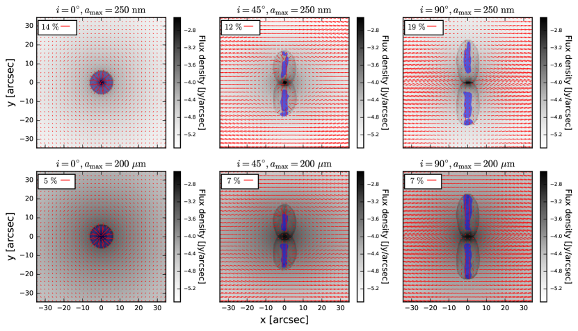
Figure 8: Synthetic flux density maps (grey coded) with a wavelength of $\lambda=1.3\ \rm{mm}$ and a distance of $140\ \rm{pc}$ overlaid with vectors of linear polarization considering RAT alignment for inclination angles of $i=0^{\circ}$ (left column), $i=45^{\circ}$ (middle column), and $i=90^{\circ}$ (right column) and maximal dust grain radii of $a_{\rm{max}}=250\ nm$ (top row) and $a_{\rm{max}}=200\ {\rm{\mu m}}$ (bottom row). The length of the vectors depends on the degree of linear polarization. For better comparison the colorbar is fixed between $F_{\rm{min}}=-4.0\ \log_{10}(\rm{Jy/arcsec})$ and $F_{\rm{max}}=-2.0\ \log_{10}(\rm{Jy/arcsec})$ in all plots. The blue colored areas indicate where the polarization vectors represent the helical magnetic field morphology of the outflow itself according to LOS analysis.

Dust grains in the ISM are very likely to be of submicron size (see Sect. 3). In contrast to this, grains inside protoplanetary disks and outflows can differ significantly in size from grains in the diffuse ISM. Grain growth in the disk is expected to enrich the surrounding environment with dust grains of sizes up to $\lesssim 1\ \rm{mm}$ (e.g. Sahai et al. 2006; Hirashita & Li 2013). The choice of upper dust grain size may significantly affect the resulting synthetic intensity and polarization maps and subsequently the predictions for future observational missions. Hence, in this section we investigate the impact of the inclination angle together with how the upper dust grain size effects intensity and linear polarization.
The sizes of dust grains are most probably not evenly distributed in all regions. Larger dust grains coagulating in the disk are expected to get blown out along the outflow lobes. Near the tip of the outflow lobes, the dust grain sizes are re-processed towards smaller radii because of high temperature and pressure in this area. This complexity is beyond the scope of the current analysis and so we here follow a simpler approach with a constant upper cut-off radius of $a_{\rm{max}}$ throughout the model space. We pre-calculated dust cross sections for two additional dust models with distinct cut-off radii of $a_{\rm{max}}=250\ \rm{nm}$ in accordance to the standard MRN model (see Sect. 3) and an extreme case with $a_{\rm{max}}=200\ \rm{\mu m}$. We repeated the postprocessing of the MHD data for the RT pipeline as described in Sect. 5.
Fig 8 shows the resulting map of intensity at a wavelength of $1.3\ \rm{mm}$ overlaid with the vectors of linear polarization dependent on inclination and the different dust grain models. As for Fig. 7, we assume a distance of $140\ \rm{pc}$ to the outflow system. Areas with a positive detection of the helical magnetic field component according to the LOS analysis presented in the previous section are marked in blue. These findings agree independently of the applied dust grain model or inclination due to the fact that only the regions close to the symmetry axis of the outflow lobes are accessible by observations. The same applies for the orientation of linear polarization. The pattern of the polarization vectors shown in Fig. 8 (see Fig. 7 bottom row) is in good agreement with the results presented in Sect. 6.2. The overall polarization pattern calculated with an upper dust grain size of $a_{\rm{max}}=250\ \rm{nm}$ (Fig. 8 top row) and $a_{\rm{max}}=200\ \rm{\mu m}$ (Fig. 8 bottom row) are rather similar to each other. There are differences regarding intensity and degree of linear polarization. In contrast to the other maps with $a_{\rm{max}}=250\ \rm{nm}$ synthetic images with an upper dust grain size of $a_{\rm{max}}=200\ \rm{\mu m}$ (Fig. 8 right column) show a higher intensity with an reduced degree of linear polarization. However, the finding that the helical magnetic field component within the outflow lobes should in principle be detectable for an wavelength of $\lambda=1.3\ \rm{\mu m}$ holds independent of applied dust grain model (see also Fig. 7).

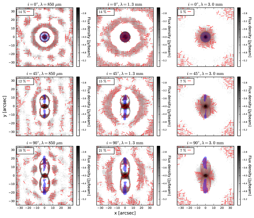
Figure 9: Synthetic $ALMA$ flux density maps (grey coded) for a wavelength of $\lambda=850\ \rm{\mu m}$ (left column), $\lambda=1.3\ \rm{mm}$ (middle column), and $\lambda=3.0\ \rm{mm}$ (right column) at a distance of $140\ \rm{pc}$ overlaid with vectors of linear polarization considering RAT alignment for inclination angles of $i=0^{\circ}$ (top row), $i=30^{\circ}$ (middle row), and $i=60^{\circ}$ (bottom row). The length of the vectors depends on the degree of linear polarization. For better comparison the colorbar is fixed between $F_{\rm{min}}=-4.0\ \log_{10}(\rm{Jy/beam})$ and $F_{\rm{max}}=-2.0\ \log_{10}(\rm{Jy/beam})$ in all plots. The blue colored areas indicate where the helical magnetic field morphology is potentially be detectable accord LOS analysis.

9 Synthetic observations

In contrast to the ideal scenarios of the prevision sections, realistic observing conditions considering instrumental and atmospheric effects may further complicate the interpretation of polarization data. In this section we translate our synthetic intensity and polarization data into observational maps. Here the focus is on determining whether the areas where the helical field is dominating linear polarization presented in Sect’s. 7 and 8 would still be detectable by actual observations.
With regard to the limitations of wavelength without a flip of polarization vectors (see Sect. 6.1) as well the expected field of view (see Fig. 7 bottom row) of the post-processed MHD outflow simulation the $ALMA$ (Brown et al. 2004) observatory provides the necessary equipment to constrain the observable parameter of linear polarization, and subsequently, that of the underlying magnetic field morphology. We calculate polarization and intensity data for three typical wavelength of $850\ \rm{\mu m}$, $1.3\ \rm{mm}$, and $3.0\ \rm{mm}$ for dust grains with an upper cut-off of radius of $a_{\rm{max}}=2\ \rm{\mu m}$ of the size distribution. We assume a mosaic observation with an object-observer distance of $140\ \rm{pc}$. The Stokes $I$, $Q$, and $U$ maps were separately processed, making use of the standard $ALMA$ reduction software $CASA$ (McMullin et al. 2007) with the simobserve and clean task. Here, we apply a resolution of $1\ \rm{arcsec}$, an observation time of five hours, and we included thermal noise as well as precipitable water vapor of $0.5\ \rm{mm}$ mimicking the atmosphere.
Initially, the observability of the outflow lobes in the resulting $I$, $Q$, and $U$ maps was heavily disturbed by the very bright inner disk regions due to the dominating influence of the overall PSF. Since these regions are very compact, most of the emission is in the longest baseline. Hence, we limit the visibility (in the uv-plane) in order to take care of these bright disk regions. Finally, we combined the $I$, $Q$, and $U$ maps to create synthetic maps of intensity and linear polarization with Eq’s. 11 and 12.
Fig. 9 shows the resulting flux density maps overlaid with the scaled vectors of linear polarization for our simulated $ALMA$ data. In the synthetic observations with a wavelength of $\lambda=850\ \rm{\mu m}$ (Fig. 9 left column), the detectable intensity covers just the disk region and the very edges of the outflow lobes. This is related to the point spread function (PSF), dominated by the brightest contributions located in the inner disk and the followup cleaning process (see McMullin et al. 2007). However, these detectable regions still coincide with the regions determined with the LOS analysis (see Sect. 7). Although the $ALMA$ instrument seems to be barely suitable to detect a polarization signal emerging from our post-processed MHD simulation at $\lambda=850\ \rm{\mu m}$, it is in principle possible to detect a polarization signal from within the outflow lobe since the detectability increases even further for even longer wavelength. At a wavelength of $\lambda=1.3\ \rm{mm}$ (Fig. 9 middle column) the interior of the outflow lobe and subsequently the helical magnetic field morphology is partially observable for low inclination angles. Even with an increase in inclination angle up to $90^{\circ}$ the helical field would still be partly accessible by polarization measurements with $ALMA$. For $\lambda=3.0\ \rm{mm}$ (see Fig. 9 right column) the observable intensity completely covers the outflow lobes. The only exception is an inclination angle of $90^{\circ}$. Here, the blue area of the LOS analysis is is marginally larger then the intensity observable with $ALMA$. However, as Fig. 9 shows in the right bottom panel a wavelength of $3.0\ \rm{mm}$ provides the optimal configuration to discriminate the helical magnetic field morphology embedded in the outflow lobes from the surrounding hourglass field. This is due to the largest area found with the LOS analysis coinciding with intensity and the polarization pattern minimally influenced by the PSF in the outflow lobes.

10 Discussion

10.1 Dichroic extinction versus thermal re-emission

The examination of multi-wavelength polarization measurements highlights one of the major obstacles for the interpretation from dust polarization measurements. The polarization effects of dichroic extinction and thermal re-emission contribute simultaneously to linear polarization with the preferential polarization axes perpendicular to each other. Both contributions to polarization can be calculated exactly (see Sect. 5). Here, the most relevant parameters are the cross section of dichroic extinction $\Delta C_{\rm{e}}$ and absorption $\Delta C_{\rm{a}}$. In the applied dust model of Sect. 3 the cross $\Delta C_{\rm{e}}$ dominates toward shorter wavelength while for absorption $\Delta C_{\rm{a}}$ increase with wavelength. Hence, one can expect an flip of $90^{\circ}$ towards longer wavelength.
Dust temperature and number density also vary along the LOS and different regions of the system dominate the overall polarization calculation as a function of wavelength resulting in an additional offset of the projected magnetic field direction. As a result of this, a characteristic area where both effects cancel each other out manifests as a eminently obvious ring structure of minimal polarization shown in the left column of Fig. 3. Polarization maps of that type are prone to misinterpretation. Several physical effects such as regions with a reduced dust density, a large amount of crossing magnetic field lines along the LOS, or a randomization of dust grain orientation by a high velocity stream (e.g. Rao et al. 1998), may also account for a reduction in the degree of linear polarization.
An even more ambiguous polarization pattern represents the result shown in the middle column of Figs. 3 and 7. A helical magnetic field morphology in the interior of the outflow lobe is expected from theoretical predictions. Hence, by comparing the alignment behavior shown in Fig. 2 with the orientation vectors of linear polarization in the middle panels of Figs. 3 one might easily conclude to probe the distinct helical field of the overall magnetic field morphology. However, the LOS analysis introduced in Sect. 7 reveals a different picture. The particular polarization map at a wavelength of $\lambda=93\ \mu m$ matches just the hourglass component of the magnetic field morphology throughout the polarization map as a result of two different polarization effects. In the outer parts it is thermal reemission while close to the outflow lobes the polarization vectors switch by $90^{\circ}$ due to dichroic extinction. The helical magnetic field morphology can not be traced up to a wavelength of about $\lambda\gtrapprox 600\ \rm{\mu m}$.
These ambiguities become irrelevant with decreasing inclination angles. A polarization signal does not emerge from aligned dust grains when the LOS and the magnetic field direction are parallel (see Eq. 3). Consequently, the hourglass field cannot contribute to linear polarization with a LOS along the outflow direction (compare Fig. 2 a.). Hence, for low inclination angles the helical morphology of the magnetic field is not hidden by the hourglass component and can be identified unambiguously.
In Chapman et al. (2013), they investigate the correlation between the direction of the magnetic field lines in low-mass cores and the bipolar outflows and not detectable of differently shaped magnetic fields. The direction and degree of linear polarization observed is in good agreement with that in presented in Sect. 6.1. Especially, the decreasing degree of linear polarization towards the outflow (see Figs. 7 and 8) is consistent with our result. This confirms the validity of the approach of creating synthetic polarization maps by combining dust combining dust continuum RT with dust grain alignment theory to create synthetic polarization maps.

10.2 Alignment-specific polarization pattern

The RT simulations reveal a marginal contribution of IDG alignment to the net polarization, making RAT clearly the dominant alignment mechanism in this outflow scenario. Since RAT alignment depends also on the alignment efficiency $Q_{\Gamma}(\epsilon)$ (see Eq. 5), where $\epsilon$ is the angle between radiation field and magnetic field, one could also expect to detect this characteristic in the resulting polarization pattern (see Andersson et al. 2011; Reissl et al. 2016). However, in the post-processing of the MHD simulation such an angle-dependent effect is not noticeable because of the local dust temperature distribution and its contribution to the overall radiation field. In contrast to a point-like source, the heated and dense surface of the outflow lobes acts like a light bulb that illuminates the model space from more than one direction (compare Fig. 2 left panel) and the radiation field is more diffuse as it would be for a point-like source. Hence the angle-dependency of $Q_{\Gamma}(\epsilon)$ becomes less relevant.

10.3 The role of dust grain size

For the maps in Fig. 8 (upper row) we used the standard MRN model with an cut off of $a_{\rm{max}}=250\ \rm{nm}$. In this model RT calculations showed that the maximum size of RAT alignment (see Sect. 5) exceeded the upper cut of radius in a considerable amount of regions in the outflow simulation ($a_{\rm{alg}}\geq a_{\rm{max}}$). One could thus expect a lower degree of linear polarization. However, due to the lack of larger dust grains the model with $a_{\rm{max}}=250\ \rm{nm}$ (8 top row) is optically thinner compared to other models with larger cut off radii. This results in less extinction and consequently flux and polarization remains similar to the model with $a_{\rm{max}}=2\ \rm{\mu m}$ shown in Fig. 7 (bottom row). The model with $a_{\rm{max}}=200\ \rm{\mu m}$ is shown in Fig 8 (bottom row). Dust grains of maximal size are quite rare in the dust mixture because of the standard MRN power-law size distribution (see Sect. 3). However, the higher re-emission cross section $C_{\rm{a}}$ of larger dust grains at mm wavelengths compensates their lower abundance. This results in a higher flux for the model with $a_{\rm{max}}=200\ \rm{\mu m}$ compared to the other models by a factor of $\approx 2$. Additionally, with increasing cut-off radii the polarization along the LOS becomes also rapidly dominated by larger dust grains. However, in the range of wavelength where $\lambda\approx a$ the cross section of re-emitted polarization has its minimum. Consequently, the peak value of linear polarization is reduced for a model with $a_{\rm{max}}=200\ \rm{\mu m}$ by a factor between $2$ and $3$.

10.4 Constraints to observational equipment

The synthetic polarization maps show that the helical field morphology in the interior of the outflow lobes is not easily accessible by polarization measurements with aligned dust grains (see Figs. 7 and 8). This holds even more reconsidering the limitations of actual observational equipment. The instrument $HAWC+$ mounted on the airborne telescope $SOFIA$ (Dowell et al. 2013) is capable of linear polarization measurements. However, its field of view (between $2.7\times 1.7\ \rm{arcmin}$ and $8.0\times 6.1\ \arcmin{arcmin}$) and spectral coverage ($53\ \rm{\mu m}-214\ \rm{\mu m}$) makes it not suitable to observe the particular outflow scenario presented in this paper (see also Sect. 10). Additionally, the instruments limit of polarized intensity does not allow to probe the interior of the outflow. In order to utilize the full field of view in the available $HAWC+$ bands, our protostellar outflow object should also be in a distance between $10\ \rm{pc}$ and $40\ \rm{pc}$. However, there is no star forming region within such a distance (Preibisch & Smith 1997). Furthermore, as shown in Sect. 6.1, the regime of wavelengths, where the transition of dominant polarization mechanism from dichroic extinction to thermalre-emission takes place, coincide with the $HAWC+$ bands. Consequently, the measurements with the $HAWC+$ instrument would be inconclusive with regard to the actually traced magnetic field direction. We performed an additional LOS analysis for all $HAWC+$ bands which reveal that the observed polarization pattern would completely represent the projected outside hourglass magnetic field morphology. The helical field inside the outflow lobe can not be detected within the $HAWC+$ bands. The detectability of the helical magnetic field morphology is just given in the far-IR, sub-mm and mm regime of wavelength (see Sect.7).
In contrast to $SOPHIA/HAWC+$, the $ALMA$ telescope can actually probe the interior of the outflow lobes especially in the sub-mm and mm regime. Here, the limitations lie in the influence of the brightest regions in the disk regions and their influence to the observability of the outflow lobes. While the outside regions can not completely be covered even at a wavelength of $\lambda=3.0\ \rm{mm}$ the polarization of the outflow lobe, especially that emerging from the helical magnetic field component is accessible by $ALMA$ for that wavelength. However, we used an ideal non-turbulent MHD simulation for the RT calculations. Although ALMA observations can probe the interior of the outflow lobes this task may be challenged in more realistic environments with additional blending by turbulent motions.

11 Summary and conclusions

We presented synthetic polarization maps from the mid-IR to the mm wavelength regime of a post-processed MHD protostellar outflow simulation. The post-processing was performed with the RT code POLARIS (Reissl et al. 2016). Here, we considered different grain alignment theories, inclination angles, and dust models in order to constrain the parameters that allow to detect the helical magnetic field component in the outflow lobes embedded in a larger hourglass shaped field of the surrounding medium.
The conclusions of this study are as follows:

1. With increasing wavelength the transition between dichroic extinction and thermal re-emission manifests itself in a flip of the orientation angles of $90^{\circ}$ in linear polarization. Additionally, areas where these transition takes place are depolarized and the magnetic field morphology is no longer accessible by observations. The polarization maps are completely dominated by thermal re-emission at $\lambda\simeq 600\ \rm{\mu m}$ and the orientation in polarization pattern stays fixed. The low polarization degree in the outflows is in accordance with the findings of Tomisaka (2011) and Chapman et al. (2013).

2. We developed a heuristic method to identify the origin of the polarisation. We show that the helical magnetic field structure inside the outflow lobe is observable only close to the symmetry axis of the lobe and at the tip of the outflow. Outside these regions the polarisation emerges from the hourglass magnetic field structure in the foreground of the outflow.

3. The alignment of dust grains does not result in polarization when the LOS is parallel to the magnetic field direction. This effect is independent of considered dust grain alignment theory and wavelength. However, this fact is of advantage in the particular case of the post-processed molecular outflows MHD simulation because it allows us to probe the interior of the outflow lobes for low inclination angles.

4. Synthetic polarization maps have been calculated considering different grain alignment theories. The polarization is dominated by RAT alignment that produces polarization degrees of a few $1\%$ to $\sim 10\%$ in agreement with observation. In contrast, the IDG alignment does not produce measurable polarization degrees.

5. Probing the interior of the outflow lobes depends on the maximum size of the dust grain distribution. We simulated polarization map with a power law size distribution considering different upper grain sizes. A composition with larger grains leads to higher intensity but also a lower polarization and vise versa. However, the overall pattern of linear polarization seems to be independent of the cut-off radius. We expect the best observability for an upper cut-off in the order of $\approx 1\ \rm{\mu m}$.

6. From the observational point of view the best conditions to probe the interior of the outflow lobes is under inclination angles close to $0^{\circ}$ or $90^{\circ}$ for a wavelengths from the far-IR ($\lambda\gtrapprox 600\mu m$) to the mm regime.

7. The interior of the outflow, i.e. the helical field structure, cannot be probed with $SOPHIA/HAWC+$, since in the available bands the polarisation is dominated by the hourglass field in the foreground of the outflows.

8. In contrast, ALMA observations should potentially allow to probe even the interior of the outflow lobes and subsequently to distinguish between the helical magnetic field in the outflow and the larger hourglass shaped field structure in the surrounding medium.

As shown in this paper, the origin of the polarization remains ambiguous at best and cannot be easily inferred from observations alone. However, progress is possible by creating physically well motivated synthetic polarization maps and designing methods of analysis allows to constrain the parameter of possible helical field detection for future observations.