Sine-Gordon soliton as a model for Hawking radiation of moving black holes and quantum soliton evaporation

Abstract

The intriguing connection between black holes’ evaporation and physics of solitons is opening novel roads to finding observable phenomena. It is known from the inverse scattering transform that velocity is a fundamental parameter in solitons theory. Taking this into account, the study of Hawking radiation by a moving soliton gets a growing relevance. However, a theoretical context for the description of this phenomenon is still lacking. Here, we adopt a soliton geometrization technique to study the quantum emission of a moving soliton in a one-dimensional model. Representing a black hole by the one soliton solution of the sine-Gordon equation, we consider Hawking emission spectra of a quantized massless scalar field on the soliton-induced metric. We study the relation between the soliton velocity and the black hole temperature. Our results address a new scenario in the detection of new physics in the quantum gravity panorama.

I Introduction

During the last ten years, analogue gravity systems have attracted major interest in the scientific community Visser et al. (2005). These models aim at providing valuable scenarios to test inaccessible features of quantum gravity, as the Hawking radiation emission by black holes (BHs) Hawking (1987). Furthermore, the recent observation of gravitational waves (GWs) emitted by colliding BHs Abbott et al. (2016a, b) shaded new light and opened unexplored roads towards the search for quantum effects in gravity Mukhanov and Winitzky (2007), as the Hawking’s BH evaporation Sakalli and Ovgun (2016a); *sakalli2015; *sakalli2015bis; *sakalli2016bis. Indeed, quantum BH emission might be observed by the concomitant monitoring of the BH collisions by gravitational and electromagnetic antennas. However, the collision process changes the original Hawking’s framework.

Originally, Hawking considered quantum fields in a stationary BH background, the Schwarzschild metric, and discovered that BHs emit thermal radiation and evaporate. His paper appeared exactly one year after a trailblazing article by Ablowitz, Kaup, Newell and Segur (AKNS), that cast new light on nonlinear waves by establishing the general method to solve classes of nonlinear field equations Ablowitz et al. (1973a, b). Surprisingly, AKNS classes generate a metric and define an event horizon (EH). Indeed, it is known in the field of the nonlinear waves that integrable systems, which can be solved exactly by the inverse scattering transform (IST), describe a Riemannian surface with constant negative curvature Bullough and Caudrey (1980); Sasaki (1979).

Recently, Hawking radiation analogues from solitons were considered in a huge variety of physical contexts, including light Leonhardt and Philbin (2008); Steinhauer (2014); Bermudez and Leonhardt (2016); Tettamanti et al. (2106); Di Mauro Villari et al. (2016), ultracold gases Garay et al. (2000); Garay (2002); Becker et al. (2008); Volkoff and Fischer (2016), water and sound waves Unruh (1981); Gerace and Carusotto (2012). Here, we study the geometrization of soliton equation by considering a canonical field quantization in the classical background of the Sine-Gordon (SG) soliton metric. Indeed, the $1+1$ dimensional Sine-Gordon (SG) equation

$$\phi_{tt}-\phi_{xx}+m^{2}\sin(\phi)=0$$ (1)

is a nonlinear model that exhibits a Riemannian surface with constant negative curvature.

In this frame, the SG equation can be considered the AKNS counterpart of a two dimensional gravitational theory. Two dimensional theories of gravity are useful models to understand the quantum properties of higher-dimensional gravity. These theories capture essential features of higher-dimensional counterparts, and in particular have black hole solutions and Hawking radiation Giddings and Strominger (1993); Mandal et al. (1991); Witten (1991); Callan et al. (1992). The link between the 1+1 dimensional gravity and the SG model introduces further simplifications since the quantum properties of this equation have been largely studied Faddeev and Korepin (1977); Zamolodchikov and Zamolodchikov (1979). As we shall recall in the next section, the integrability condition of SG equation determines a metric, with a coordinate singularity, which defines an EH. In particular 1+1 dimensional BHs can be realized as solitons of the SG equation Gegenberg and Kunstatter (1997) and it has been shown with a one loop perturbative computation that this BH emits thermal radiation Vaz and Witten (1995); Kim and Won (1995).

In this paper, we show that SG soliton emits thermal particles with a specific Hawking temperature, finding the way the temperature changes with the velocity of the SG-BH. Afterward, we perform two different kinds of quantization, one for a massless scalar field and another for the soliton itself, and obtain their Hawking emission spectra. In both cases, we discover that an observer on the soliton tail detects a thermal radiation with a temperature directly proportional to the soliton speed. Furthermore, we analyze the temperature detected by an observer at rest by adding a Doppler effect.

Our paper is organized as follows: in sec. II we review the geometrization of the SG model; we show the connection between a soliton solution of an AKNS system and a metric on a two dimensional surface. In sec. III we study the BH metric induced by the SG equation and introduce suitable coordinate systems for the field quantization. In section IV we quantize massless scalar fields on the soliton background. In section V we quantize the SG soliton following the Faddeev semiclassical quantization Faddeev and Korepin (1977), and show that the sine-gordon BH evaporates. Conclusions are drawn in section VI. A short appendix furnishes a minimal mathematical background to forms and curvature.

II Sine-Gordon geometrization

We start reviewing the way integrable nonlinear equations generates surfaces with constant negative curvature Bullough and Caudrey (1980). By considering the SG equation defined in Eq. (1), we perform the coordinate transformation

$$\chi=\frac{m}{2}(x+t),\;\;\theta=\frac{m}{2}(x-t)$$ (2)

and get

$$\phi_{\chi\theta}=\sin\phi.$$ (3)

As originally stated by Ablowitz, Kaup, Newel and Segur Ablowitz et al. (1973b), for Eq. (3) the following system defines the scattering problem

$$\begin{cases}\mathbb{V}_{\chi}=\hat{L}\mathbb{V}\\ \mathbb{V}_{\theta}=\hat{M}\mathbb{V}\end{cases},$$ (4)

where $\hat{L}$ and $\hat{M}$ are $2\times 2$ matrices, defining the Lax pair for Eq. (3). $\mathbb{V}$ is a vector. This system corresponds to the integrable Pfaffian system Flanders (1963) (see appendix for an introduction to forms and surfaces)

$$\,\mathrm{d}\mathbb{V}=\hat{\Omega}\mathbb{V},\quad\mathbb{V}=\left(\begin{array}[]{c}V_{1}\\ V_{2}\end{array}\right),$$ (5)

where $\hat{\Omega}$ is a traceless matrix

$$\hat{\Omega}=\hat{L}\,\mathrm{d}\chi+\hat{M}\,\mathrm{d}\theta=\left(\begin{array}[]{cc}\omega_{1}&\omega_{2}\\ \omega_{3}&-\omega_{1}\end{array}\right),$$ (6)

with the matrix elements $\omega_{i}$ given by Bullough and Caudrey (1980)

$$\omega_{1} =-\frac{1}{2}\lambda\,\mathrm{d}\chi-\frac{1}{2\lambda}\cos(\phi)\,\mathrm{d}\theta,$$ (7)

$$\omega_{2} =-\frac{1}{2}\phi_{\chi}\,\mathrm{d}\chi-\frac{1}{2\lambda}\sin(\phi)\,\mathrm{d}\theta,$$

$$\omega_{3} =\frac{1}{2}\phi_{\chi}\,\mathrm{d}\chi-\frac{1}{2\lambda}\sin(\phi)\,\mathrm{d}\theta,$$

where $\lambda$ is the spectral parameter of the SG scattering problem Ablowitz et al. (1973b). Following Sasaki (1979), the arclength of the induced Riemannian surface is written in terms of the matrix elements $\omega_{i}$ as follows Flanders (1963); Bullough and Caudrey (1980)

$$\,\mathrm{d}s^{2}=(\omega_{2}+\omega_{3})^{2}+(2\omega_{1})^{2}=$$ (8)

$$=\lambda^{2}\,\mathrm{d}\chi^{2}+2\cos(\phi)\,\mathrm{d}\chi\,\mathrm{d}\theta+\frac{1}{\lambda^{2}}\,\mathrm{d}\theta^{2}.$$

Eq. (8) defines the constant negative curvature metric induced by the ISM associated to the SG equation (3). By changing the coordinates set as in the following, we write the first fundamental form $\,\mathrm{d}s^{2}$ as Bullough and Caudrey (1980)

$$\,\mathrm{d}s^{2}=\sin^{2}\Bigl{(}\frac{\phi}{2}\Bigl{)}\,\mathrm{d}\tau^{2}+\cos^{2}\Bigl{(}\frac{\phi}{2}\Bigl{)}\,\mathrm{d}\xi^{2},$$ (9)

which results to be associated with a SG equation of the form

$$\phi_{\xi\xi}-\phi_{\tau\tau}=\sin(\phi),$$ (10)

where

$$\left\{\begin{array}[]{c}\xi=\lambda\chi+\lambda^{-1}\theta\\ \tau=\lambda\chi-\lambda^{-1}\theta\end{array}\right..$$ (11)

Thus the metric tensor is

$$\hat{g}=\left(\begin{array}[]{cc}g_{\tau\tau}&g_{\xi\tau}\\ g_{\tau\xi}&g_{\xi\xi}\end{array}\right)=\left(\begin{array}[]{cc}\sin^{2}\frac{\phi}{2}&0\\ 0&\cos^{2}\frac{\phi}{2}\end{array}\right).$$ (12)

However, $\,\mathrm{d}s^{2}$ in Eq. (9) is not Lorentz invariant and it does not lead to a Schwarzschild-like metric. Following Gegenberg and Kunstatter (1997), in order to obtain a Minkowski-like metric, we perform a Wick rotation $\tau\rightarrow i\tau$ and obtain the elliptic SG (ESG) equation:

$$\phi_{\xi\xi}+\phi_{\tau\tau}=\sin(\phi),$$ (13)

whose corresponding metric is

$$\,\mathrm{d}s^{2}=-\sin^{2}\Bigl{(}\frac{\phi}{2}\Bigl{)}\,\mathrm{d}\tau^{2}+\cos^{2}\Bigl{(}\frac{\phi}{2}\Bigl{)}\,\mathrm{d}\xi^{2}.$$ (14)

III The Sine-Gordon soliton black hole

We show that the one-soliton solution of the ESG equation determines a BH metric.

The well known forward-propagating one-soliton solution of the Eq. (10) is

$$\phi(\xi,\tau)=4\arctan\left\{\exp\left[\gamma\left(\xi-\beta_{s}\tau\right)\right]\right\},$$ (15)

with $\gamma=(1-\beta_{s}^{2})^{-1/2}$ and $0<\beta_{s}<1$ the soliton velocity Ablowitz et al. (1973c). The backward-propagating one-soliton solution gives the same treatise with $-1<\beta_{s}<0$, by substituting $\beta_{s}$ in $-\beta_{s}$ in what follows. For this reason, we can choose solution (15) without loss of generality. Eq. (15) is also solution of Eq. (13) with

$$\gamma=(1+\beta_{s}^{2})^{-1/2}.$$ (16)

We adopt Eq. (16) hereafter. Substituting Eq. (15) in Eq. (14), we have

$$ds^{2}=ds^{2}_{1sol}=-\operatorname{sech}^{2}(\rho)d\tau^{2}+\tanh^{2}(\rho)d\xi^{2},$$ (17)

with $\rho=\gamma(\xi-\beta_{s}\tau)$. Following Gegenberg and Kunstatter (1997), we adopt various coordinate transformations: first from $(\tau,\xi)$ to $(\mathcal{T},\rho)$, with $\rho$ as defined above and

$$\mathcal{T}=\tau-\frac{1}{\beta_{s}}\{\tanh^{-1}[\gamma^{-1}\tanh(\rho)]-\gamma^{-1}\rho\}.$$ (18)

Next, we transform $(\mathcal{T},\rho)$ to $(\mathcal{T},r)$ by

$$r=\frac{1}{\gamma}\operatorname{sech}(\rho).$$ (19)

The result of the transformation is the line element

$$ds^{2}=(\beta_{s}^{2}-r^{2})d\mathcal{T}^{2}-(\beta_{s}^{2}-r^{2})^{-1}dr^{2}.$$ (20)

Eq. (20) is the metric of a 1+1 dimensional BH with EH at $r_{g}:=\beta_{s}$. Figures 1 and 2 show the EH positions
$\rho_{g}=\operatorname{arcsech}(\gamma r_{g})$ on the soliton profiles and energy densities $\mathcal{E}$, respectively for different velocities $\beta_{s}$. The energy density, at fixed $t$, is defined as follows Faddeev and Korepin (1977):

$$\mathcal{E}=\frac{1}{2}(\partial_{\xi}\phi_{s})^{2}+[1-cos(\phi_{s})].$$

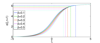
Figure 1: (Color online) The sine-Gordon soliton at fixed time $\tau=1$, varying the velocity $\beta_{s}$. The positions of the EHs $\rho_{g}=m\gamma(\xi_{g}-\beta_{s}\tau)$ are in dashed lines.

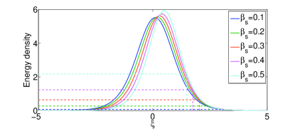
Figure 2: (Color online) The soliton energy density at various velocities $\beta_{s}$, at fixed time $\tau=1$. The positions of the EHs $\rho_{g}=m\gamma(\xi_{g}-\beta_{s}\tau)$ are in dashed lines.

It is now convenient to introduce two new sets of coordinates: the modified Regge-Wheeler coordinate, that we call the slug coordinate in analogy with the tortoise coordinate, as usually reported Hawking (1987); Mukhanov and Winitzky (2007), and the Kruskal-Szekeres coordinates.
We get the slug coordinate $r^{*}(r)$ according to

$$dr^{*}=(\beta_{s}^{2}-r^{2})^{-1}dr,$$ (21)

so that

$$r^{*}(r)=\frac{1}{\beta_{s}}\tanh^{-1}\left(\frac{r}{\beta_{s}}\right)=\frac{1}{2\beta_{s}}\ln\left(\frac{\beta_{s}+r}{\beta_{s}-r}\right).$$ (22)

Eq. (20) then becomes

$$ds^{2}=[\beta_{s}^{2}-r^{2}(r^{*})][d\mathcal{T}^{2}-(dr^{*})^{2}].$$ (23)

The slug coordinate is singular at $r=\beta_{s}$ and it is defined on the exterior of the BH when $\rho\to\pm\infty$ and $r\to 0$. In fact, as $r$ approaches $\beta_{s}$, $r^{*}$ goes to $+\infty$, while far away from the BH $r^{*}\to 0$ as $r\to 0$.
Introducing the slug lightcone coordinates

$$\tilde{u}=\mathcal{T}-r^{*},\quad\tilde{v}=\mathcal{T}+r^{*},$$ (24)

we write Eq. (20) as

$$ds^{2}=[\beta_{s}^{2}-r^{2}(\tilde{u},\tilde{v})]d\tilde{u}d\tilde{v}.$$ (25)

The slug lightcone coordinates are singular and they span only the exterior of the black hole. To describe the entire spacetime, we need another coordinate system. In order to be consistent with literature, we refer to them as the Kruskal-Szekeres (KS) coordinates . From Eq. (22) and Eq. (24) it follows that

$$\beta_{s}^{2}-r^{2}=(\beta_{s}+r)^{2}\exp[\beta_{s}(\tilde{u}-\tilde{v})].$$ (26)

The BH metric thus becomes

$$ds^{2}=[\beta_{s}+r(\tilde{u},\tilde{v})]^{2}e^{\beta_{s}(\tilde{u}-\tilde{v})}d\tilde{u}d\tilde{v}.$$ (27)

In the KS lightcone coordinates, defined as

$$u=\frac{e^{\beta_{s}\tilde{u}}}{\beta_{s}}\text{,}\quad v=-\frac{e^{-\beta_{s}\tilde{v}}}{\beta_{s}},$$ (28)

Eq. (27) takes the form

$$ds^{2}=[\beta_{s}+r(\tilde{u},\tilde{v})]^{2}dudv,$$ (29)

and it is regular at $r=\beta_{s}$. The singularity occurring in the ESG-soliton metric is, as the Schwarzschild one, a coordinate singularity, which can be removed by a coordinate transformation. The KS coordinates, indeed, span the entire spacetime.

IV Massless scalar field quantization

We consider a field quantization on the classical soliton background metric. We first analyze a massless scalar field with the action

$$S[\phi]=\frac{1}{2}\int g^{\mu\nu}\partial_{\mu}\phi\partial_{\nu}\phi\sqrt{-g}\,d^{2}\underline{x},$$ (30)

where $g^{\mu\nu}$ represents the inverse of a general metric tensor $g_{\mu\nu}$, $g$ is the determinant of $g_{\mu\nu}$ and $\underline{x}=(x^{0},x^{1})$. The action in Eq. (30) is conformally invariant, and in terms of lightcone slug coordinates and lightcone KS coordinates (29) it reads

$$S[\phi]=\int\partial_{\tilde{u}}\phi\partial_{\tilde{v}}\phi\,d\tilde{u}d\tilde{v},$$ (31)

$$S[\phi]=\int\partial_{u}\phi\partial_{v}\phi\,dudv.$$

We write the solution of the scalar field equation in terms of the lightcone slug coordinates

$$\phi=\tilde{A}(\tilde{u})+\tilde{B}(\tilde{v}),$$ (32)

and in the lightcone KS coordinate as

$$\phi=A(u)+B(v),$$ (33)

where $A$, $\tilde{A}$ and $B$, $\tilde{B}$ are arbitrary smooth functions. In correspondance of the tail of the soliton, i.e., far away from the EH, the mode expansion of the field is

$$\hat{\phi}=\int_{0}^{\infty}\frac{d\Omega}{2\sqrt{\pi\Omega}}\bigl{[}e^{-i\Omega\tilde{u}}\hat{b}^{-}_{\Omega}+e^{+i\Omega\tilde{u}}\hat{b}^{+}_{\Omega}\bigl{]}+\text{left moving}.$$ (34)

In Eq. (34) the left moving part is given by the terms weighted by $e^{\pm i\Omega\tilde{v}}$ in the mode expansion. The vacuum state $\ket{0_{B}}$, defined by $\hat{b}^{-}_{\Omega}\ket{0_{B}}=0$, is the Boulware vacuum (BV) and does not contain particles for an observer located far from the EH. However, as the slug coordinate is singular at horizon, the BV is also singular at the EH.

To obtain a vacuum state defined over the entire spacetime, we expand the field operator in terms of the KS lightcone coordinates

$$\hat{\phi}=\int_{0}^{\infty}\frac{d\omega}{2\sqrt{\pi\omega}}\bigl{[}e^{-i\omega u}\hat{a}^{-}_{\omega}+e^{i\omega u}\hat{a}^{+}_{\omega}\bigl{]}+\text{left moving}.$$ (35)

The creation and annihilation operators $\hat{a}^{\pm}_{\omega}$ determine the Kruskal vacuum (KV) state $\hat{a}^{-}_{\omega}\ket{0_{K}}=0$. The KV is regular on the horizon and corresponds to true physical vacuum in the presence of the BH.
For a remote observer the KV contains particles. To determine their number density, we follow the original calculations of Hawking and Unruh with the only difference in the definition of the KS coordinates (see chapters 8 and 9 of Mukhanov and Winitzky (2007) for details).
We find that the remote observer moving with the soliton tail sees particles with the thermal spectrum

$$\braket{\hat{N}_{\Omega}}=\bra{0_{K}}\hat{b}^{+}_{\Omega}\hat{b}^{-}_{\Omega}\ket{0_{K}}=\left[\exp\left(\frac{2\pi\Omega}{\beta_{s}}\right)-1\right]^{-1}\delta(0).$$ (36)

If we consider a finite volume quantization we can put $V=\delta(0)$ Mukhanov and Winitzky (2007) and we obtain the number density

$$n_{\Omega}=\left[\exp\left(\frac{2\pi\Omega}{\beta_{s}}\right)-1\right]^{-1},$$ (37)

corresponding to the temperature

$$T_{H}=\frac{\beta_{s}}{2\pi}.$$ (38)

In Fig. 3, we show the radiance $B(\Omega)=\Omega^{3}n_{\Omega}$. We observe that for a static soliton ($\beta_{s}=0$) we get $T_{H}=0$. This result may appear in contradiction with the Hawking original work, where he considered the emission from a static BH. However the result in eq. (38) is coherent with the structure of the metric induced by the SG equation, where the singularity occurs for $r=r_{g}=\beta_{s}$ and no emission can be observable for $r_{g}=0$. This dependence of the Hawking radiations on the translation velocity is peculiar of soliton dynamics Martina et al. (1998) and it is related to the structure of the spectral parameter in the IST Ablowitz et al. (1973a, b).

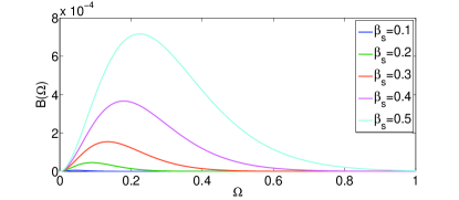
Figure 3: (Color online) Spectral radiance for massless fields varying $\beta_{s}$.

IV.1 Hawking temperature in the laboratory frame

Unlike the Schwarzschild BH, the ESG soliton is not static, but translates with velocity $\beta_{s}$. The frequency $\Omega$ seen by an observer at rest with respect to the soliton contains a Doppler shift. Letting $\Omega_{s}$ be the frequency emitted by the soliton in (36), the frequency measured by an observed moving with velocity $-\beta_{s}$ with respect to the soliton, and located at an angle $\theta_{s}$ with respect to the soliton direction is

$$\Omega_{o}=\frac{1-\beta_{s}\cos\theta_{s}}{\sqrt{1-\beta_{s}^{2}}}\Omega_{s}.$$ (39)

In the collinear case $\theta_{s}=0$, and we have

$$\frac{\Omega_{o}}{\Omega_{s}}=\sqrt{\frac{1-\beta_{s}}{1+\beta_{s}}}.$$ (40)

The corresponding Hawking temperature is (for small $\beta_{s}$)

$$T_{H}=\frac{\beta_{s}}{2\pi}\sqrt{\frac{1-\beta_{s}}{1+\beta_{s}}}\simeq\frac{\beta_{s}}{2\pi}(1-\beta_{s}).$$ (41)

This calculation also applies to a massive bosonic field, as the number density spectrum depends only on the statistics Crispino et al. (2008). In the case of a fermionic field the theory is similar, but the number density spectrum follows the Fermi-Dirac statistics Hawking (1987).

V Soliton Quantization

Previously we studied the BH evaporation following the works of Hawking and Unruh in Hawking (1987); Unruh (1976). Now, we analyze a quantum perturbation of the BH metric given by the classical soliton solution of the ESG equation, and we obtain a BH evaporation without the interaction with a massless scalar field. We start from

$$\phi\simeq\phi_{s}+\phi_{1},$$ (42)

where $\phi_{s}$ is the classical solution in Eq. (15) and $\phi_{1}$ represents a weak field perturbation. We consider the conformally invariant action

$$S[\phi]=\int\,\left[\frac{1}{2}g^{\mu\nu}\partial_{\mu}\partial_{\nu}\phi+cos(\phi)\right]\sqrt{-g}\,d^{2}x,$$ (43)

which leads to a field equation

$$g^{\mu\nu}\partial_{\mu}\partial_{\nu}\phi+\sin(\phi)=0.$$ (44)

The solutions of Eqs. (10,13) differ for a Wick rotation. In other words, one passes from the SG soliton to the ESG one by the transformation

$$\tau\rightarrow i\tau,\;\;\beta_{s}\rightarrow-i\beta_{s}.$$ (45)

We perform the inverse Wick rotation, i.e., $\tau\rightarrow-i\tau$,
$\beta_{s}\rightarrow i\beta_{s}$, passing from the ESG to the SG, and substitute Eq. (42) into Eq. (44), hence we obtain

$$g^{\mu\nu}\partial_{\mu}\partial_{\nu}\phi_{1}+\cos(\phi_{s})\phi_{1}=0,$$ (46)

where we neglect terms $O(\phi_{1}^{2})$. This equation expresses the interaction between a massive particle and the gravitational field, because the weak quantum field $\phi_{1}$ obeys a generalized Klein-Gordon equation with squared mass $\cos(\phi_{s})$ depending on the soliton, and thus on the metric. Recalling Eq. (15), we have

$$g^{\mu\nu}\partial_{\mu}\partial_{\nu}\phi_{1}+\cos\{4\arctan[\exp(\rho)]\}\phi_{1}=0.$$ (47)

For an observer located on the tail of the soliton
($\rho\to\infty$), the field equation reduces to

$$g^{\mu\nu}\partial_{\mu}\partial_{\nu}\phi_{1}+\phi_{1}=0,$$ (48)

while for an observer on the horizon ($\rho\to\rho_{g}$), we have

$$g^{\mu\nu}\partial_{\mu}\partial_{\nu}\phi_{1}+F(\rho)\phi_{1}=0,$$ (49)

with $F(\rho)$ given by

$$F(\rho)|_{\rho\sim\rho_{g}}\simeq 1+\frac{5}{2}\gamma^{2}\beta_{s}^{2}-5\gamma^{2}\beta_{s}^{2}\sqrt{1-\gamma^{2}v^{2}}(\rho-\rho_{g}).$$ (50)

Eq. (50) truncated at the order zero in $\rho-\rho_{g}$, i.e., exactly on the horizon, leads to

$$F\simeq 1+\frac{5}{2}\gamma^{2}\beta_{s}^{2}.$$ (51)

Due to the inverse Wick rotation, even if the action is conformally invariant, the quantization is not straightforward. We need to adapt both the slug and the KS lightcone coordinates in Eqs. (24,28) to the rotated system. We obtain

$$r^{*}(r) =\int_{0}^{r}\frac{dr^{\prime}}{\beta_{s}^{2}+r^{\prime 2}}=\frac{i}{2\beta_{s}}\ln{\Biggl{(}\frac{i\beta_{s}+r}{i\beta_{s}-r}\Biggl{)}},$$ (52)

$$\tilde{u} =\mathcal{T}-ir^{*},\quad\tilde{v}=\mathcal{T}+ir^{*},$$

$$u =-\frac{e^{-\beta_{s}\tilde{u}}}{\beta_{s}},\quad v=\frac{e^{\beta_{s}\tilde{v}}}{\beta_{s}}.$$

Since the action (43) is conformally invariant, we thus write the field equation as follows

$$\partial_{\tilde{u}}\partial_{\tilde{v}}\phi_{1}+\phi_{1}=0\,\,\,\text{slug lightcone},$$ (53)

$$\partial_{u}\partial_{v}\phi_{1}+F\phi_{1}=0\,\,\,\text{ K-S lightcone},$$

Eqs. (53) have exponential solution

$$\phi_{1}\propto e^{i(K-\Omega_{K})\tilde{u}-i(K+\Omega_{K})\tilde{v}},$$ (54)

$$\phi_{1}\propto e^{i(k-\omega_{k})u-i(k+\omega_{k})v},$$

with the following dispersion relations,

$$\Omega_{K} =\sqrt{K^{2}+1},$$ (55)

$$\omega_{k} =\sqrt{k^{2}+F^{2}}.$$

From now on, we omit the $K$ and $k$ indices. We write the quantum fields as follows

$$\hat{\phi}_{0} =\frac{1}{2\pi}\int_{0}^{\infty}\frac{d\Omega}{\sqrt{\Omega}}\,[\hat{b}^{-}_{\Omega}e^{i(K-\Omega)\tilde{u}-i(k+\Omega)\tilde{v}}+\hat{b}^{+}_{\Omega}e^{-i(K-\Omega)\tilde{u}+i(K-\Omega)\tilde{v}}]=$$ (56)

$$=\frac{1}{2\pi}\int_{0}^{\infty}\frac{d\omega}{\sqrt{\omega}}\,[\hat{a}^{-}_{\omega}e^{i(k-\omega)u-i(k+\omega)v}+\hat{a}^{+}_{\omega}e^{-i(k-\omega)u+i(k+\omega)v}],$$

where, as in the non interacting case, the annihilation operators $\hat{b}^{-}_{\Omega}$ and $\hat{a}^{-}_{\omega}$ define the Boulware vacuum $\ket{0_{B}}$ and the Kruskal vacuum $\ket{0_{K}}$, respectively. The operators $\hat{a}_{\omega}^{\pm}$ and $\hat{b}_{\Omega}^{\pm}$ are related by the Bogolyubov transformations

$$\hat{b}^{-}_{\Omega}=\int_{0}^{\infty}d\omega\,(\alpha_{\Omega\omega}\hat{a}^{-}_{\omega}-\beta_{\Omega\omega}\hat{a}^{+}_{\omega}).$$ (57)

By substituting this in Eq. (56), we find

$$\frac{1}{\sqrt{\omega}}\int_{-\infty}^{\infty}d\tilde{u}d\tilde{v}\,e^{i[\Omega(\tilde{u}+\tilde{v})-K(\tilde{u}-\tilde{v})}e^{-i[\omega(u+v)+k(u-v)]}=\int_{0}^{\infty}\frac{d\Omega^{\prime}}{\sqrt{\Omega^{\prime}}}\,\alpha_{\Omega^{\prime}\omega}[2\pi\delta(\Omega-\Omega^{\prime})]^{2},$$ (58)

hence we obtain

$$\alpha_{\omega\Omega}=\frac{1}{2\pi V}\sqrt{\frac{\Omega}{\omega}}\int d\tilde{u}d\tilde{v}e^{iu(k-\omega)-iv(k+\omega)}e^{-i\tilde{u}(K-\Omega)+iv(k+\Omega)}.$$ (59)

Seemingly for $\beta_{\Omega\omega}$, we have

$$\beta_{\omega\Omega}=-\frac{1}{2\pi V}\sqrt{\frac{\Omega}{\omega}}\int d\tilde{u}d\tilde{v}e^{-iu(k-\omega)+iv(k+\omega)}e^{-i\tilde{u}(K-\Omega)+iv(k+\Omega)}.$$ (60)

Using now the KS coordinate (52), after lengthy but straightforward calculations, we find

$$\alpha_{\Omega\omega} =\frac{1}{2\pi V}\frac{\Omega}{\omega}e^{\pi\Omega/\beta_{s}}e^{iF(\Omega,K,\omega,k)}\Gamma\Bigl{[}i\frac{\Omega+K}{\beta_{s}}\Bigl{]}\Gamma\Bigl{[}i\frac{\Omega-k}{\beta_{s}}\Bigl{]},$$ (61)

$$\beta_{\Omega\omega} =\frac{1}{2\pi V}\frac{\Omega}{\omega}e^{-\pi\Omega/\beta_{s}}e^{iG(\Omega,K,\omega,k)}\Gamma\Bigl{[}i\frac{\Omega+K}{\beta_{s}}\Bigl{]}\Gamma\Bigl{[}i\frac{\Omega-k}{\beta_{s}}\Bigl{]}.$$

It follows that $\alpha_{\Omega\omega}$ and $\beta_{\Omega\omega}$ obey the useful relation

$$|\alpha_{\Omega\omega}|^{2}=e^{4\pi\Omega/\beta_{s}}|\beta_{\Omega\omega}|^{2}.$$ (62)

Therefore we can compute the expectation value of the $b$-particle number operator $\hat{N}_{\Omega}=\hat{b}^{+}_{\Omega}\hat{b}^{-}_{\Omega}$ in the Kruskal vacuum Mukhanov and Winitzky (2007), and obtain the number density

$$n_{\Omega}=\Bigl{[}\exp\Bigl{(}\frac{2\Omega}{T_{H}}\Bigr{)}-1\Bigl{]}^{-1}.$$ (63)

This corresponds to an emitted radiation with twice the frequency with respect to the simple massless case, of which spectral radiance $B(\Omega)=\Omega^{3}n_{\Omega}$ is reported in figure 4. We observe that the Hawking temperature is equal to Eq. (38) for the massless scalar field. This is expected since the surface gravity is the same. For a moving observer with respect to the soliton the Hawking temperature, for small $\beta_{s}$, reads

$$T_{H}=\frac{\beta_{s}}{2\pi}\sqrt{\frac{1-\beta_{s}}{1+\beta_{s}}}\simeq\frac{\beta_{s}}{2\pi}(1-\beta_{s}).$$ (64)

Eq. (64) provides the Hawking temperature of soliton evaporation in this toy model.

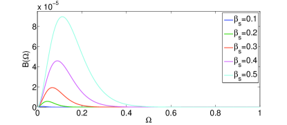
Figure 4: (Color online) Spectral radiance for massive fields varying the soliton velocity.

VI Conclusions

We adopted the geometrization of the ESG model and reported on the connection between the one-soliton solution of the 1+1-dimensional elliptic sine-Gordon equation and a metric with a Schwarzschild-like coordinate singularity. We determined the BH metric and, by suitable coordinate systems, we eliminated the singularity and obtained a regular metric on the EH. We quantized a massless scalar field and found the thermal radiation detected by an observer far away on the BH exterior. We obtained that the temperature is proportional to the soliton velocity. We analyzed the temperature detected by an observer in the laboratory frame, by a Doppler effect. We studied also the quantum soliton evaporation, and found the corresponding spectrum.

Our analysis allows to predict the Hawking radiation for a moving 1+1 dimensional BH and shows that the velocity affects the temperature and the corresponding emitted thermal spectrum. In a BH collisional process one can hence expect a frequency shift of the emitted photon concomitant with the variation of spiraling velocity of the BHs. The resulting chirp of the emitted photons may have a clear and detectable signature in the electromagnetic spectrum. Analogues of these processes may be eventually simulated in the long-range interactions between optical solitons pairs recently observed over astronomical distances Jang et al. (2013), or similar optical experiments Bekenstein et al. (2015); Roger et al. (2016).

Our results may be extended to any metric induced by AKNS systems, hence to many different physical models to conceive experimentally realizable analogues for studying Hawking evaporation of moving black holes.

Appendix: minimal introduction to forms, Pfaff problems and curvature

A 1-form $\Omega=X\,\mathrm{d}x+T\,\mathrm{d}t$ is a combination of the differentials $\,\mathrm{d}x$ and $\,\mathrm{d}t$, which have to be retained as elements of a basis. $X$ and $T$ can be matrices with the same size, or also operators. A 2-form is a combination of the symbols (“exterior products”) $\,\mathrm{d}x\wedge\,\mathrm{d}t$ and
$\,\mathrm{d}t\wedge\,\mathrm{d}x=-\,\mathrm{d}x\wedge\,\mathrm{d}t$. One can obtain a 2-form from a 1-form by the differential operator $\,\mathrm{d}$:

$$\,\mathrm{d}\Omega=\frac{\partial X}{\partial t}\,\mathrm{d}t\wedge\,\mathrm{d}x+\frac{\partial T}{\partial x}\,\mathrm{d}x\wedge\,\mathrm{d}t=\left(-\frac{\partial X}{\partial t}+\frac{\partial T}{\partial x}\right)\,\mathrm{d}x\wedge\,\mathrm{d}t\text{,}$$ (65)

which can be kept in mind by letting
$\,\mathrm{d}x\wedge\,\mathrm{d}x=\,\mathrm{d}t\wedge\,\mathrm{d}t=0$, so that terms like $\partial_{x}X$ and $\partial_{t}T$ do not appear in $\,\mathrm{d}\Omega$.
One can also obtain a 2-form by the exterior product $\Omega\wedge\Omega$ again by $\,\mathrm{d}x\wedge\,\mathrm{d}x=\,\mathrm{d}t\wedge\,\mathrm{d}t=0$

$$\Omega\wedge\Omega=XT\,\mathrm{d}x\wedge\,\mathrm{d}t+TX\,\mathrm{d}t\wedge\,\mathrm{d}x=[X,T]\,\mathrm{d}x\wedge\,\mathrm{d}t$$ (66)

with $[X,T]$ the commutator.
By using forms, the AKNS integrability condition

$$\frac{\partial X}{\partial t}-\frac{\partial T}{\partial x}+[X,T]=0\text{,}$$ (67)

reads as

$$\,\mathrm{d}\Omega-\Omega\wedge\Omega=0.$$ (68)

For some authors, using forms has the advantage of a more compact notation as the explicit coordinates $x$ and $t$ do not appear in (68). Eq. (68) is referred to a Pfaffian integrability condition, or Pfaff problem.

Forms are directly connected to the curvature of surfaces. If one considers a surface, and a local point vector ${\bf P}$ on the surface, let ${\bf e}_{1}$ and ${\bf e}_{2}$ the orthogonal tangent vectors. For infinitesimal motion on the surface $\,\mathrm{d}{\bf P}$

$$\,\mathrm{d}{\bf P}=\sigma^{1}{\bf e}_{1}+\sigma^{2}{\bf e}_{2}\text{,}$$ (69)

where $\sigma^{1}$ and $\sigma^{2}$ contain the differentials of the adopted coordinates and are hence 1-form. $\sigma^{1}\wedge\sigma^{2}$ is the elemental area on the surface. When one moves of an amount $\,\mathrm{d}{\bf P}$, ${\bf e}_{1,2}$ changes of amounts $\,\mathrm{d}{\bf e}_{1,2}$. One considers a surface such that $\,\mathrm{d}{\bf e}_{1}=\omega{\bf e}_{2}$ and $\,\mathrm{d}{\bf e}_{2}=-\omega{\bf e}_{1}$ where $\omega$ depends on the shape of the surface, contains the differentials of the coordinate systems, and is a 1-form named the connection one form. One finds the following equation

$$\,\mathrm{d}\omega=-K\sigma^{1}\wedge\sigma^{2}$$ (70)

where $K$ is the Gaussian curvature. $\omega$, $\sigma^{1}$ and $\sigma^{2}$ are one forms that fix all the properties of the surface. In the particular case $K=-1$, one has from (70)

$$\,\mathrm{d}\omega=\sigma^{1}\wedge\sigma^{2}.$$ (71)

By using (71) and considering the matrix 1-form Sasaki (1979)

$$\Omega=\left(\begin{array}[]{cc}-\frac{1}{2}\sigma^{2}&\frac{1}{2}(\omega+\sigma^{1})\\ \frac{1}{2}(-\omega+\sigma^{1})&\frac{1}{2}\sigma^{2}\end{array}\right),$$ (72)

one finds the Pfaff system in Eq. (68). In other words, considering the integrability condition (68), and retaining the element of $\Omega$ as the forms of a two-dimensional surface, Eq. (68) implies that the surface has a constant negative curvature $K=-1$. Hence integrability produces pseudospherical surfaces, i.e., surfaces of constant negative curvature.

References

- Visser et al. (2005) M. Visser, C. Barceló, and S. Liberati, Living Rev. Rel. 8, 12 (2005).
- Hawking (1987) S. W. Hawking, Nature 248, 1038 (1987).
- Abbott et al. (2016a) B. P. Abbott et al. (LIGO Scientific Collaboration and Virgo Collaboration), Phys. Rev. Lett. 116, 061102 (2016a).
- Abbott et al. (2016b) B. P. Abbott et al. (LIGO Scientific Collaboration and Virgo Collaboration), Phys. Rev. Lett. 116, 241103 (2016b).
- Mukhanov and Winitzky (2007) V. F. Mukhanov and S. Winitzky, Introduction to Quantum Effects in Gravity (Cambridge University Press, 2007).
- Sakalli and Ovgun (2016a) I. Sakalli and A. Ovgun, Gen. Rel. Grav. 48 (2016a).
- Sakalli and Ovgun (2015a) I. Sakalli and A. Ovgun, EPL 110, 10008 (2015a).
- Sakalli and Ovgun (2015b) I. Sakalli and A. Ovgun, Eur. Phys. J. Plus 130 (2015b).
- Sakalli and Ovgun (2016b) I. Sakalli and A. Ovgun, Eur. Phys. J. Plus 131 (2016b).
- Ablowitz et al. (1973a) M. Ablowitz, D. Kaup, A. Newell, and H. Segur, Phys. Rev. Lett. 31, 125 (1973a).
- Ablowitz et al. (1973b) M. Ablowitz, D. Kaup, A. Newell, and H. Segur, Phys. Rev. Lett. 30, 1262 (1973b).
- Bullough and Caudrey (1980) R. Bullough and P. Caudrey, Solitons (Spriger-Verlag, 1980).
- Sasaki (1979) R. Sasaki, Phys. Lett. 71A, 390 (1979).
- Leonhardt and Philbin (2008) U. Leonhardt and T. Philbin, ArXiv:0803.0669 (2008).
- Steinhauer (2014) J. Steinhauer, Nat. Phys. 10, 864 (2014).
- Bermudez and Leonhardt (2016) D. Bermudez and U. Leonhardt, Phys. Rev. A 93, 053820 (2016).
- Tettamanti et al. (2106) M. Tettamanti, S. Cacciatori, A. Parola, and I. Carusotto, ArXiv:1603.04702 (2106).
- Di Mauro Villari et al. (2016) L. Di Mauro Villari, E. M. Wright, F. Biancalana, and C. Conti, ArXiv:1608.04905 (2016).
- Garay et al. (2000) L. J. Garay, J. R. Anglin, J. I. Cirac, and P. Zoller, Phys. Rev. Lett. 85, 4643 (2000).
- Garay (2002) L. J. Garay, Int. J. Theor. Phys. 41, 2073 (2002).
- Becker et al. (2008) C. Becker, S. Stellmer, P. Soltan-Panahi, S. Dorscher, M. Baumert, E. Richter, J. Kronjager, K. Bongs, and K. Sengstock, Nat. Phys. 4, 496 (2008).
- Volkoff and Fischer (2016) T. J. Volkoff and U. R. Fischer, Phys. Rev. D 94, 024051 (2016).
- Unruh (1981) W. G. Unruh, Phys. Rev. Lett. 46, 1351 (1981).
- Gerace and Carusotto (2012) D. Gerace and I. Carusotto, Phys. Rev. B 86, 144505 (2012).
- Giddings and Strominger (1993) S. Giddings and A. Strominger, Phys. Rev. D 47, 2454 (1993).
- Mandal et al. (1991) G. Mandal, A. M. Sengupta, and S. R. Wadia, Mod. Phys. Lett. A 06, 1685 (1991).
- Witten (1991) E. Witten, Phys. Rev. D 44, 314 (1991).
- Callan et al. (1992) C. G. Callan, S. B. Giddings, J. A. Harvey, and A. Strominger, Phys. Rev. D 45, R1005 (1992).
- Faddeev and Korepin (1977) L. D. Faddeev and V. Korepin, Phys. Rep. 42, 3 (1977).
- Zamolodchikov and Zamolodchikov (1979) A. B. Zamolodchikov and A. B. Zamolodchikov, Ann. of Phys. 120, 253 (1979).
- Gegenberg and Kunstatter (1997) J. Gegenberg and G. Kunstatter, Phys. Lett. B 43, 274 (1997).
- Vaz and Witten (1995) C. Vaz and L. Witten, Cl. and Quant. Grav. 12, 2607 (1995).
- Kim and Won (1995) S. Kim and T. K. Won, Phys. Lett. B 361, 38 (1995).
- Flanders (1963) H. Flanders, Differential forms (Academic Press, 1963).
- Ablowitz et al. (1973c) M. Ablowitz, D. Kaup, A. Newell, and H. Segur, The Inverse Scattering Transform-Fourier Analysis for Nonlinear Problems (Massachusetts Institute of Technology, 1973).
- Martina et al. (1998) L. Martina, O. K. Pashaev, and G. Soliani, Phys. Rev. D 58, 084025 (1998).
- Crispino et al. (2008) L. C. B. Crispino, A. Higuchi, and G. E. A. Matsas, arXiv:0710.5373 (2008).
- Unruh (1976) W. G. Unruh, Phys. Rev. D 14, 870 (1976).
- Jang et al. (2013) J. K. Jang, M. Erkintalo, S. G. Murdoch, and S. Coen, Nat. Photon. 7 (2013).
- Bekenstein et al. (2015) R. Bekenstein, R. Schley, M. Mutzafi, C. Rotschild, and M. Segev, Nat. Phys. 11, 872 (2015).
- Roger et al. (2016) T. Roger, C. Maitland, K. Wilson, N. Westerberg, D. Vocke, E. Wright, and D. Faccio, Nat. Commun. 7, 13492 (2016).