Mott metal-insulator transition in the Doped Hubbard-Holstein model

Abstract

Motivated by the current interest in the understanding of the Mott insulators away from half filling, observed in many perovskite oxides, we study the Mott metal-insulator transition (MIT) in the doped Hubbard-Holstein model using the Hatree-Fock mean field theory. The Hubbard-Holstein model is the simplest model containing both the Coulomb and the electron-lattice interactions, which are important ingredients in the physics of the perovskite oxides. In contrast to the half-filled Hubbard model, which always results in a single phase (either metallic or insulating), our results show that away from half-filling, a mixed phase of metallic and insulating regions occur. As the dopant concentration is increased, the metallic part progressively grows in volume, until it exceeds the percolation threshold, leading to percolative conduction. This happens above a critical dopant concentration $\delta_{c}$, which, depending on the strength of the electron-lattice interaction, can be a significant fraction of unity. This means that the material could be insulating even for a substantial amount of doping, in contrast to the expectation that doped holes would destroy the insulating behavior of the half-filled Hubbard model. Our theory provides a framework for the understanding of the density-driven metal-insulator transition observed in many complex oxides.

I Introduction

It is well known that the half filled Hubbard model is a Mott insulatorMott when the strength of the on-site Coulomb interaction $U$ exceeds a critical value. Within the Hubbard model, the Mott insulating state can exist only at half filling, and just a single hole is supposed to destroy the antiferromagnetic insulating ground state, turning it into a ferromagnetic metal as suggested by the Nagaoka TheoremNagaoka , strictly true in the infinite $U$ limit.

Quite early on, the Mott insulator LaTiO₃ was thought to be a prototypical example of the Nagaoka Theorem, where the undoped LaTiO₃ is an antiferromagnetic insulator, as predicted for the half-filled Hubbard model, but both the antiferromagnetism as well as the insulating behavior are quickly destroyed with the introduction of a small number of holes via the addition of extra oxygenTaguchi or via $Sr$ substitution (with as little as $x\approx 0.05$ for La_1-xSr_xTiO₃)Tokura . Indeed, a large number of perovskite oxides have since been found to turn into metals upon hole doping, but only after a substantial amount of hole concentration has been introduced into the system. At the same time, scanning tunneling microscopy images of these doped oxides show mixed phases in the nanoscale, meaning that there is no clear phase separation with a single boundary separating the two phases, but rather that the two phases break into intermixed nanoscale puddles. In addition, transport measurements follow percolative scaling laws with doping and temperature, further confirming the existence of the mixed phaseSWCheong ; Schneider ; Mydosh .

From a theoretical point of view, there have been many studies of the doped Mott insulators Kotliar96 ; XGWen ; Kotliar86 ; Onoda ; Tremblay2009 ; Dagotto2 ; Becca ; Gang ; Cosentini ; Arrigoni ; Zitzler ; Aichhorn ; Visscher ; Andriotis ; Emery ; Hellberg ; Gimm ; Luchini ; Shih ; Igoshev ; Balents , largely for models in two dimensions (2D), because numerical methods such as Quantum Monte Carlo are more feasible there. However, the results vary depending on the methods used. In the 2D Hubbard model, results from quantum Monte Carlo calculationsDagotto2 ; Becca found no evidence for phase separation, consistent with the “somewhat” exact results of SuGang . However, other authors using the fixed-node quantum Monte Carlo methodCosentini or the Hartree-Fock mean-field approximationArrigoni have suggested phase separation in large regions of the parameter space. Phase separation at small doping levels was also found in the dynamical mean field calculationZitzler and the variational cluster perturbation theory works Aichhorn . There are much fewer studies of the phase separation for the Hubbard model in 3D, although the existence of the phase separation there was suggested by the early works of VisscherVisscher in the 1970s. The recent Hartree-Fock calculations in 3DIgoshev and the dynamical mean-field theory (DMFT) workMillis , strictly valid for infinite dimensions, have found phase separation in a large region of parameter space, as did the work of Andriotis et al.Andriotis , who used the coherent-potential approximation and the Bethe lattice.

Phase separation in the closely related $t$-$J$ model has also been investigated because of its relevance to the cuprate superconductors. The phase separation has been reported for all values of $J/t$ by several authorsEmery ; Hellberg ; Gimm , while some authors find it only for larger values of $J/t$ Luchini ; Shih . There is thus a general consensus for the phase separation in the $t$-$J$ model with a large $J/t$ and the non-half-filled band, where the system separates into two regions, viz., an undoped antiferromagnetic region and a carrier-rich ferromagnetic region.

All these theoretical works do not include the coupling of lattice to the electrons, which is an important ingredient in the physics of many perovskite oxides, where a strong Jahn-Teller coupling plays a critical role in the behavior of the material. In this paper, we study the Hubbard-Holstein model with the Hartree-Fock method, which includes both the Coulomb interaction as well as the electron-lattice coupling. We study the energetics of the various magnetic phases including the paramagnetic and the spiral phase (which incorporates the AFM and FM phases as special cases) and compute the phase stability in the doped system near half filling. For small number of dopants (electrons or holes), the system phase separates into an undoped antiferromagnetic insulator and a carrier-rich, ferro or spiral magnetic, metallic phase. As the dopant concentration is increased, the metallic part grown in volume, and eventually at a critical dopant concentration, the percolation threshold is reached and the system becomes a conductor. The critical concentration for this percolative Mott metal-insulator (MIT) transition is studied for varying interaction parameters, and the theoretical results are connected with the existing experiments in the literature.

II Model

We consider the Hubbard-Holstein model for a cubic lattice

$${\cal H} = \sum_{\langle ij\rangle\sigma}t_{ij}(c_{i\sigma}^{\dagger}c_{j\sigma}+H.c.)+U\sum_{i}{n}_{i\uparrow}{n}_{i\downarrow}$$ (1)

$$+ \sum_{i}(\frac{1}{2}KQ^{2}_{i}-gQ_{i}n_{i})-\mu\sum_{i\sigma}n_{i\sigma},$$

which contains both the Coulomb interaction and the electron-lattice coupling terms. Here $c_{i\sigma}^{\dagger}$ is the electron creation operator at site $i$ with spin $\sigma$, $n_{i\sigma}=c^{\dagger}_{i\sigma}c_{i\sigma}$ is the number operator, $t_{ij}$ is the hopping amplitude between nearest-neighbor sites denoted by $\langle ij\rangle$, $U$ is the onsite Coulomb repulsion, $Q_{i}$ is the lattice distortion at site $i$, $K$ and $g$ are, respectively, the stiffness and the electron-lattice coupling constants, and $\mu$ is the chemical potential that controls the carrier concentration. Taking the nearest-neighbor hopping integral as $t_{ij}=-t$, there are two parameters in the Hamiltonian, viz., $U/t$ and $\lambda\equiv g^{2}/(KW)$, where $W=12|t|$ is the band width and $\lambda$ is the effective electron-lattice coupling strength. Note that we have considered the static Holstein modelHolstein , which contains a simpler version of the local lattice interaction such as the Jahn-Teller interaction, and, in addition, it does not contain any phonon momentum dependence.

The key problem to study is the energy of the ground state and the stability of the various phases as a function of the carrier concentration away from the half filling. Both magnetic (ferro, antiferro, or spiral) as well as non-magnetic phases are considered. In fact, all these solutions are special cases of the spiral phase, which is conveniently described in terms of a site-dependent local spin basis set described by the unitary transformationArrigoni

$$d^{\dagger}_{i\sigma}=\sum_{\sigma^{\prime}}(e^{-i\vec{\sigma}\cdot\vec{\alpha_{i}}/2})_{\sigma\sigma^{\prime}}\ c^{\dagger}_{i\sigma^{\prime}},$$ (2)

where $\vec{\alpha_{i}}$ is the site dependent spin rotation angle. The spiral phase is described by $\vec{\alpha_{i}}=(\vec{q}\cdot\vec{R_{i}})~{}\hat{x}$, where $\hat{x}$ is the spin rotation axis, $\vec{R}_{i}$ is the site position, and $\vec{q}\equiv(q_{x},q_{y},q_{z})$ is the modulation wave vector of the spiral state. The ferro, para, as well as the antiferromagnetic states, considered in this work, are all special cases of the spiral state. Explicitly, $\vec{q}=0$ for the ferro or paramagnetic state, while it is $\pi(1,1,1)$ for the Néel antiferromagnetic state.

In the new basis, the Hamiltonian (1) remains unchanged except for the first term, which becomes ${\cal H}_{ke}=\sum_{\langle ij\rangle,\sigma\sigma^{\prime}}(t^{\sigma\sigma^{\prime}}_{ij}d^{\dagger}_{i\sigma}d_{j\sigma^{\prime}}+H.c.)$, where the hopping is now spin-dependent

$$t^{\sigma\sigma^{\prime}}_{ij}=(e^{i\vec{q}\cdot(\vec{R_{i}}-\vec{R_{j}})\sigma_{x}/2})_{\sigma\sigma^{\prime}}t_{ij},$$ (3)

and in the remaining terms in (1), the number operators are redefined to mean $n_{i\sigma}=d^{\dagger}_{i\sigma}d_{i\sigma}$. Making the Bloch transformation into momentum space

$$d^{\dagger}_{\vec{k}\sigma}=\frac{1}{\sqrt{N}}\sum_{i}e^{i\vec{k}.\vec{R_{i}}}d^{\dagger}_{i\sigma},$$ (4)

and using the Hartree-Fock approximation: $n_{1}n_{2}=\langle n_{1}\rangle n_{2}+\langle n_{2}\rangle n_{1}-\langle d_{1}^{\dagger}d_{2}\rangle d_{2}^{\dagger}d_{1}-\langle d_{2}^{\dagger}d_{1}\rangle d_{1}^{\dagger}d_{2}-\langle n_{1}\rangle\langle n_{2}\rangle+\langle d_{1}^{\dagger}d_{2}\rangle\langle d_{2}^{\dagger}d_{1}\rangle$, we get the quasi-particle Hamiltonian

$${\cal H}(\vec{k})=\left[{\begin{array}[]{*{20}c}T_{1}(\vec{k})+U\langle n_{\downarrow}\rangle-\mu&\ -T_{2}(\vec{k})-U\langle d_{\downarrow}^{\dagger}d_{\uparrow}\rangle\\ -T_{2}(\vec{k})-U\langle d_{\uparrow}^{\dagger}d_{\downarrow}\rangle&\ \ \ T_{1}(\vec{k})+U\langle n_{\uparrow}\rangle-\mu\\ \end{array}}\right],$$ (5)

where $T_{1}(\vec{k})=-2t[\cos(k_{x}a)\cos(q_{x}a/2)+\cos(k_{y}a)\cos(q_{y}a/2)+\cos(k_{z}a)\cos(q_{z}a/2)]$, $T_{2}(\vec{k})$ is the same as $T_{1}(\vec{k})$ except that all cosine functions are replaced by sines, only the nearest-neighbor hopping $t_{ij}=-t$ has been kept in the original Hamiltonian (the unit of energy is set by $t=1$), and the expectation values $\langle d^{\dagger}_{\sigma}d_{\sigma^{\prime}}\rangle$ are to be determined self-consistently. Note that the exact form of ${\cal H}_{k}$ would depend on the spin rotation axis $\vec{\alpha}$ in the spiral phase (here chosen along $\hat{x}$). However, the final results should not depend on this choice as there is no coupling between the space and the spin coordinates. We also find from direct calculations that the exchange terms $U\langle d_{\sigma}^{\dagger}d_{-\sigma}\rangle$ appearing in Eq. (5) contribute very little to the total energy. This contribution would be exactly zero, if the spins don’t mix, so that the density matrices $\rho_{\sigma\sigma^{\prime}}\equiv\langle d_{\sigma}^{\dagger}d_{\sigma^{\prime}}\rangle$ are diagonal in the spin space.

The total energy per site is given by

$$E(\vec{q})=\frac{1}{N}\sum^{\mu}_{\vec{k}\sigma}\varepsilon_{\vec{k}\sigma}-U\langle n_{\uparrow}\rangle\langle n_{\downarrow}\rangle+U\langle d_{\uparrow}^{\dagger}d_{\downarrow}\rangle\langle d_{\downarrow}^{\dagger}d_{\uparrow}\rangle-\frac{g^{2}n^{2}}{2K},$$ (6)

where $\varepsilon_{\vec{k}\sigma}$ are the eigenvalues of the Hamiltonian in Eq. (5), the second and the third terms correct for the double counting of the Coulomb energy, and the last term is the lattice energy gain at each site, obtained from minimizing the lattice energy $\partial E/\partial Q=0$ from Eq. (1). The chemical potential is related to the number of electrons by the expression $N^{-1}\sum_{\vec{k}\sigma}\theta(\mu-\varepsilon_{\vec{k}\sigma})=n$, $N$ being the number of lattice sites. For a fixed value of doping $\delta=1-n$, where $n$ is the total number of electrons per lattice site, we have minimized the total energy $E(\vec{q})$ numerically as a function of the spiral vector $\vec{q}$ by varying each component between $0$ and $2\pi$. The minimum yields the ground state. All Brillouin zone integrations were performed with 1000 $k$-points. We restrict ourselves to the hole doping region $n\leq 1$ without loss of generality, since we have the electron-hole symmetry in the problem.

Figure 1: Ground-state energy as a function of the hole concentration $\delta$ for $U/W=1.25$ and $\lambda=0$. The lines show results for a single-site unit cell, while the crosses show the results for a double-site unit cell, which allowed for charge and spin disproportionation, but no such disproportionation was found, and the double-site results converged to the single-site results. Note that the double-site calculations allowed for the ferro or the anti-ferro phase, but not the spiral phase.

III Results

To determine the phase diagram, we calculated the ground-state energy of the system according to Eq.(6) for the given input parameters $n$, $U$, and $\lambda$. Figure (1) shows a typical plot of the ground-state energy per lattice site as a function of the hole concentration $\delta$ for different magnetic phases. As seen from the figure, the ground state is antiferromagnetic (AF) at half-filling ($\delta=0$), in agreement with the standard result for the Hubbard model. With increasing hole concentration $\delta$, the system first turns into a spiral (S) state, then into a ferromagnetic (F) state, and eventually into the paramagnetic (P) state.

Note that we have considered the spiral state in Eq. (2), which is a spin density wave (SDW) state, with the modulation wave vector $\vec{q}$, but not the charge density wave (CDW) state, which is a higher energy state and is not expected to occur in the parameter regime we are working. The CDW state is difficult to incorporate within our calculation as it requires a supercell of arbitrary size depending on the modulation wave vector of the CDW. However, we can study the CDW in a special case, viz., where the modulation $\vec{q}=(\pi,\pi,\pi)$, in which case we have two sites in the unit cell of the crystal, and we can allow for both charge and spin disproportionation between the two sublattices. Results of this calculation are also shown in Fig. (1) as crosses and they go over to the single-site results indicating the absence of any CDW for this wave vector.

We note further that the CDW state could be favored when the electron-lattice interaction is strong. We can estimate the condition for this by considering the energy of the charge-disproportionated state (a special case of the CDW) for the half-filled Hubbard-Holstein model and comparing it with the energy of the state without any charge disproportionation. In the former case, the charges on the two sublattices are $1\pm\eta$ ($\eta\leq 1$ is the charge disproportionation amplitude), and the total energy would be $E=-(g^{2}/2K)[(1+\eta)^{2}+(1-\eta^{2})]+U\eta$. The first term here is the energy gain due to lattice interaction, the second term is due to the fact that $\eta$ electrons are forced to occupy the upper Hubbard band, and we have neglected the kinetic energy difference in order to get a simple estimate. It immediately follows from this expression that such a CDW state would be favorable if $U/(W\lambda)\leq 1$. For the parameter regime relevant for the oxides, this condition is not satisfied, so that it is reasonable to omit the CDW state, which we have not considered in our work.

Figure 2: Ground-state phase diagram for the Hubbard model for the simple cubic lattice. The red dashed line separates the stable and unstable single phase regions, while the black dashed line indicates the MIT (these two lines were calculated from the total energy curve $E(\delta)$ for each $U/W$ as illustrated in Fig. (4) below). The hatched region indicates existence of the mixed phase. The dash dotted line shows the Stoner criterion result, Eq. (9), for a sinusoidal model density-of-states.

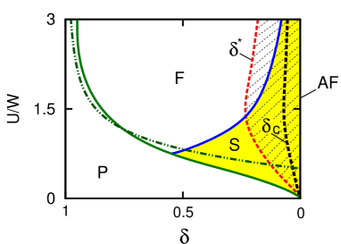
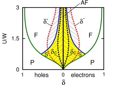
Fig. (2) shows the calculated phase diagram. For the half-filled case, there is perfect Fermi surface nesting [$\varepsilon(\vec{k}_{F})=\varepsilon(\vec{k}_{F}+\vec{q}_{n}$) = 0, $\vec{q}_{n}=\pi(1,1,1)$ is the nesting vector], which leads to an anti-ferromagnetic insulator for any value of $U$. As we move away from half filling, perfect nesting is lost and a critical value $U_{c}$ is needed for the onset of magnetic order. Below a certain hole doping $\delta$, the system goes from the paramagnetic state to a spiral state, and eventually to the ferromagnetic state, as $U$ is increased, while for a larger value of $\delta$, the system goes directly from the paramagnetic to the ferromagnetic state.

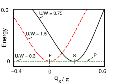
Fig. (3) shows the calculated energy as a function of the spiral wave vector for three different parameters. Note that for the paramagnetic solution corresponding to $U/W=0.3$, the energy is independent of the spiral wave vector, since the magnetic moment is zero.

Figure 3: Energy as a function of the spiral wave vector $\vec{q}=(q_{x},\pi,\pi)$ for the Hubbard model with three different Coulomb parameters, indicating the paramagnetic (P), ferromagnetic (F), or the spiral (S) ground state, depending on the strength of the Coulomb U. Here, the hole concentration is $\delta=0.6$ and the zero of the energy has been shifted to correspond to the minimum in each case.

Para-Ferro phase boundary – The boundary between the paramagnetic and the ferromagnetic phases in the Hubbard model (Fig. 2) can be understood by taking a model density of states and applying the Stoner criterion for ferromagnetic instability. We consider the sinusoidal density-of-states for each spin

$$\rho(\varepsilon)=\begin{cases}\frac{\pi}{2W}\sin\ (\varepsilon\pi/W)\hskip 8.53581pt\text{ if $0<\varepsilon<W$},\\ 0\hskip 71.13188pt\text{ else},\end{cases}$$ (7)

of bandwidth $W$. The total energy $E$ is a sum of the band energy, the Coulomb energy, and the lattice energy, which is immediately obtained from a direct integration to yield

$$E(n,m) = \frac{W}{2\pi}\big{[}\sqrt{1-x^{2}}-x\cos^{-1}x$$

$$+\sqrt{1-y^{2}} - y\cos^{-1}y\big{]}+\frac{U}{4}(n^{2}-m^{2})-\lambda n^{2},$$ (8)

where $x=1-n-m$, $y=1-n+m$, $n=n_{\uparrow}+n_{\downarrow}$ is the number of electrons, and $m=n_{\uparrow}-n_{\downarrow}$ is the spin polarization. The Fermi energies for the up and down spins are, respectively, $\varepsilon_{F\uparrow}=\pi^{-1}W\cos^{-1}x$ and $\varepsilon_{F\downarrow}=\pi^{-1}W\cos^{-1}y$. The onset of ferromegetism is determined from the Stoner criterion $U\rho(\varepsilon_{F})\geq 1$, where $\varepsilon_{F}=\pi^{-1}W\cos^{-1}(1-n)$ is the Fermi energy of the paramagnetic phase, while the spin polarization is determined by the minimization of the energy, Eq. (7), as a function of the polarization $m$. The Stoner criterion leads to the equation of the para-ferro transition line:

$$\delta=1-n=\sqrt{1-(\frac{2W}{\pi U})^{2}},$$ (9)

which is plotted as a dotted line in Fig. (2) and reproduces the trend found from the full solution of the Hubbard model for the cubic lattice. It is readily seen from Eq. (9) that for the Coulomb interaction below the critical value $U_{c}=2/\pi$, the system is paramagnetic for all values of the hole concentration $\delta$.

Figure 4: Ground-state energy as a function of the hole concentration $\delta$, indicating phase instability near half filling ($\delta=0$), and the Maxwell construction that yields the upper concentration $\delta^{*}$ for the existence of the mixed phase. The system remains an insulator for $\delta<\delta_{c}$, the percolation threshold, beyond which the metallic fraction forms a percolation network making the system a conductor. Parameters used are: $U/W=2.0$ and $\lambda=0$.

Figure 5: Phase diagram indicating the various phases as a function of carrier (electron or hole) doping $\delta$. As $\delta$ is increased starting from the AF insulator state at half-filling ($\delta=0$), the system continues to be a mixed-phase insulator, turning into a percolative metal beyond $\delta=\delta_{c}$, and eventually becoming a single-phase metal beyond $\delta^{*}$ as discussed in the text.

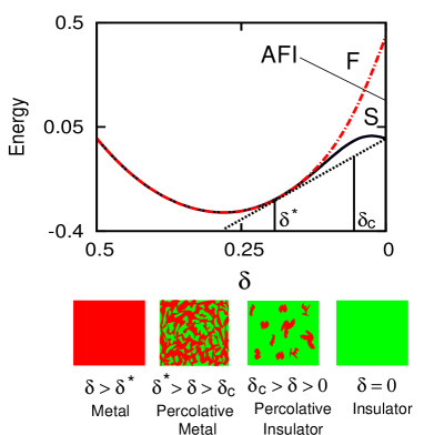
Percolative metal-insulator transition – Returning to our original Hubbard-Holstein model, as seen from Fig. (1), the ground-state energy is not everywhere convex, which indicates a phase separation, which is seen for small doping near half filling. At half filling, we have an antiferromagnetic insulator. As holes are introduced, the system phase separates into two regions, one is the anti-ferro insulating state with hole concentration zero, and the second is a spiral or ferro phase (depending on the strength of $U$) with hole concentration $\delta^{*}$. As $\delta$ is increased, so does the volume of the metallic fraction. When it exceeds a certain threshold $\delta_{c}$, given by the percolation theory, the metallic regions form a percolative network and the system conducts.

The fraction of the two phases can be obtained from the standard Maxwell construction, which is illustrated for the case of $U/W=2$ in Fig. (4). If $v_{m}(v_{i})$ is the volume fraction of the substance in the metallic (insulating) phase in the mixed phase region ($\delta^{*}<\delta<0$), then we have the two equations: $v_{m}+v_{i}=1$ and $v_{m}\delta^{*}=\delta$, which means that the metallic volume fraction linearly increases with the hole concentration, i.e., $v_{m}=\delta/\delta^{*}$. The hole concentration $\delta^{*}$ separates the mixed phase region from the single phase region and depends on the Hamiltonian parameters as seen, e.g., from Fig. (2), and it must be calculated from the total energy curve for each set of parameters from a Maxwell construction.

The Maxwell construction indicates phase separation into two separate regions consisting of single phases, separated by a single boundary. However, in the actual solids, one does not encounter such clear phase separation, but rather a mixed phase usually results, where the two phases are intermixed on the nanoscale. There are many reasons why a mixed phase could be more favorable. For example, the presence of a small amount of charged impurities because of unintentional doping could cause a deviation from charge neutrality of the two components and would impede the formation of the phase separation due to the large cost in Coulomb energy. Thus one would encounter a nanoscale inhomogeneous phase (or mixed phase) with intermixed metallic and insulating components (Coulomb frustrated phase separation)HRK . It has also been suggested that the mixed phase could even originate due to kinetic reasons, i.e., self-organized inhomogeneities resulting from a strong coupling between electronic and elastic degrees of freedom KHAHN . A large number of experiments point to the existence of the mixed phases in the oxide materials, including transport results and scanning tunneling microscopy images.Loa ; Baldini ; Ramos

The percolation threshold $v_{c}$, beyond which the metallic regions touch and the percolative conduction begins, depends on the specific model used in the percolation theory, but is typically about $v_{c}\approx 0.30$. For example, in the percolation model, where the metallic region consists of randomly-packed, overlapping spheres of radius $r$ in an insulating matrix, the critical volume fraction of the spheres for the onset of percolation is $v_{c}\approx 0.29$ and is independent of $r$ Pike . On the other hand, for the site percolation problem in the cubic lattice, the percolation threshold is about $v_{c}\approx 0.31$. The site percolation thresholds are long well known,Efros but are summarized in Table I for ready reference. We have used the value $v_{c}=0.3$ in our calculations, which is similar to the site percolation result for the cubic lattice.

	cubic	diamond	bcc	fcc	square	triangular	honeycomb
$v_{c}$	0.31	0.43	0.25	0.20	0.59	0.5	0.7

Table 1: Site percolation threshold $v_{c}$ for various lattices

Percolative conduction occurs, when the metallic volume fraction exceeds $v_{c}$, i.e., $\delta/\delta^{*}=v_{m}>v_{c}$, or

$$\delta>\delta_{c}=v_{c}\delta^{*},$$ (10)

where $\delta^{*}$ is the critical concentration, beyond which the system turns into a single-phase metal, which is either ferromagnetic or in the spin spiral state depending on the strength of $U/W$ (see Fig. (2)). For the specific parameters used in Fig. (4), the full metallic phase for $\delta>\delta^{*}$ is ferromagnetic; for intermediate values of $\delta$ between $0$ and $\delta^{*}$, the phase separation occurs between the AFI half-filled ($\delta=0$) phase and the FM metallic phase with carrier concentration $\delta^{*}$. Fig. (5) summarizes the phase diagram showing the MIT boundary. The system continues to remain an AF insulator until dopant concentration (electrons or holes) exceeds the critical value $\delta_{c}$.

Effect of electron-lattice coupling – A finite value of the electron-lattice coupling in the Hubbard-Holstein model does not change the relative energies of the various phases for a fixed concentration $n$ as already noted, since it alters the energy of each phase equally (see Eqs. (6) and (8)). The presence of charge disproportionation or a CDW ($n$ varies from site to site) would change the phase diagram; However, as we have already argued at the beginning of this Section, for parameters relevant to the oxides, the CDW phase is unlikely to occur, which we have not considered in this work. Thus the various phase regions (AF, F, P, or S) in the phase diagram, Fig. (2), remain unchanged. However, the curvatures of the ground-state total energy as a function of $n$ or $\delta$, as in Fig. (1), change, leading to the phase separation regions which now change with $\lambda$, and therefore so do the quantities $\delta_{c}$ and $\delta^{*}$. This is clearly seen from Fig. 6, where $\delta^{*}$ increases as the electron-lattice coupling strength $\lambda$ is increased.

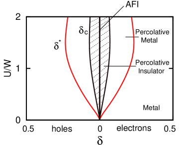
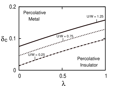
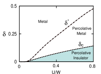
Fig. (7) shows the critical doping $\delta_{c}$ as a function of the electron-lattice coupling strength $\lambda$ for several values of $U/W$. As seen from the figure, the larger the value of $\lambda$, the higher is the dopant concentration $\delta$ needed for the transition into the metallic state. Finally, Fig. (8) shows the phase diagram in the Hubbard-Holstein model for a specific value of $\lambda$.

Figure 6: Energy vs. doping $\delta$ for different strengths of the electron-lattice coupling $\lambda=0,0.25$, and 0.6 with $U/W=1.25$. A linear term const. $\times n$ has been subtracted from the energy and the zero of the energy has been redefined to more clearly show the Maxwell construction.

Figure 7: The critical dopant concentration $\delta_{c}$ for the MIT as a function of the electron-lattice coupling strength $\lambda$. $\delta_{c}$ was obtained from the Maxwell construction (Fig. (6)) and Eq. (10).

Figure 8: Ground state phase diagram for the Hubbard-Holstein model for the simple cubic lattice for $\lambda$ = 0.6, with $\delta_{c}$ indicating the critical carrier concentration for percolative MIT, where $\delta>\delta_{c}$ is the metallic region.

perovskite oxide	critical hole	Ref.
	doping ($\delta_{c}$)
SmNiO3	0.1	SmCaNiO3
LaTiO3	0.05	Tokura
PrTiO3	0.14	RCaTiO3
NdTiO3	0.2	RCaTiO3
SmTiO3	0.24	RCaTiO3
YTiO3	0.35	YCaTiO3
LaMnO3	0.17 - 0.2	LaCaMnO3 ; LaSrMnO3
PrMnO3	0.3 - 0.5	1PrCaMnO3 ; 2PrCaMnO3 ; NdSrMnO3
NdMnO3	0.5	NdSrMnO3
LaVO3	0.176	LaSrVO32006
YVO3	0.5	YcaVO31993 ; YCdVO3

Table 2: Summary of the experimental results for the critical hole doping in the perovskite oxides for transition to the metallic state.

To make connections with the experiments, we summarize the measured critical carrier density for the MIT in several perovskite oxides from the existing literature in Table II. As these results indicate, the critical carrier concentration $\delta_{c}$ needed to transform the insulating phase into the metallic phase is a significant fraction of unity, starting from 0.05 for LaTiO₃ to as high as 0.5 for YVO₃. However, other than a few systems, where $\delta_{c}$ is as high as 0.5, for most compounds shown in Table II, it is between 0.05 and 0.2, which is the typical value of $\delta_{c}$ predicted by our theory.

Fig. (9) shows the experimental conductivity behaviorRCaTiO3 of the doped titanates RTiO₃ plotted against the bandwidth of the material as well as the same calculated from our theory. Although inclusion of the detail interactions in the Hamiltonian may be necessary for a quantitative description of a specific compound, the general trend for the onset of the MIT is well described within the Hubbard-Holstein model. As seen from Fig. (9), for a large bandwidth ($U/W$ less than a critical value), the system is a metal for all doping levels, and as $U/W$ is increased beyond a critical value, the critical carrier concentration for MIT increases, roughly linearly. This agrees with the experimental data, where Katsufuji et al.RCaTiO3 have plotted the inverse bandwidth vs. the conduction behavior for a large number of samples with different carrier concentrations in the titanates. As was argued in Ref. RCaTiO3 , the magnitude of the Coulomb $U$ may be expected to be relatively unchanged for the R_1-xCa_xTiO_3+y/2 series, allowing a direct comparison of the trends seen in theory vs. experiments.

One point to note is that Eq. (10) puts an upper limit on the critical doping $\delta_{c}\approx 0.3$, since $\delta^{*}$ can not exceed one and $v_{c}\approx 0.3$, which is what is observed for most of the samples in Table I. For carrier concentration $\delta$ as high as 0.5, as is the case for some of the samples, the crystal and electronic structures are likely changed significantly, making the model less applicable for such systems. In our theory, we have assumed that the percolative conduction occurs in the mixed phase, where the two components (metallic and insulating) occur randomly, so that the percolation theory applies. If the two components do not occur randomly, but rather that there is a tendency towards coalescing of the components, this would increase the critical value $\delta_{c}$, as more volume fraction of the metallic component will be needed before a percolation path for conduction forms.

Note that the Hartree-Fock approximation due to its mean-field nature does omit the effect of fluctuations on the phase separation. It has been shown that such quantum fluctuations can indeed modify the magnetic phase boundary within the Hubbard modelfluctu1 ; fluctu2 . However, the qualitative similarity of our theoretical results with the experiments (as seen from Fig. (9)) suggests that the Hartree-Fock results should contain the qualitative physics of the problem, while the fluctuation effects will likely alter the predicted critical doping quantitatively. The effect of the fluctuations on the phase separation remains an open question for future study.

Figure 9: Experimental conductivity data, taken from Katsufuji et al.RCaTiO3 , for the hole-doped RTiO₃ system, with the x-axis showing the renormalized bandwidth $\tilde{W}$ (ratio of the bandwidth of each RTiO₃ to that of LaTiO₃) (top) and the theoretical phase diagram from the present calculations, with the electron-lattice coupling strength $\lambda=0.6$ (bottom).

IV Summary

In summary, we studied the phase diagram and energetics of the Hubbard-Holstein model using the Hartree-Fock method. For a wide range of the Hamiltonian parameters, we found the existence of a mixed phase, consisting of an undoped component which is an anti-ferro insulator and a carrier-rich metallic phase, which is either ferromagnetic or spiral magnetic. As the carrier concentration (electrons or holes) increases with doping, the metallic portion slowly grows forming isolated islands in an insulating matrix. As the volume fraction of the metallic islands increases with carrier doping, eventually they form a percolative conducting network and the material conducts beyond the critical dopant concentration $\delta_{c}$. This happens for $\delta_{c}$ which is typically between zero and 0.2 or so, in general agreement with the experimental results. We furthermore showed that the electron-lattice interaction favors the insulating phase with respect to the metallic phase and the critical doping value increases along with the strength of the electron-lattice coupling. The general trends for the critical doping concentration for MIT predicted by our theory agrees with the existing experimental results for the hole doped perovskite oxides.

This research was supported by the U.S. Department of Energy, Office of Basic Energy Sciences, Division of Materials Sciences and Engineering under Grant No. DE-FG02-00ER45818.

References

- [1] N. F. Mott, The Basis of the Electron Theory of Metals, with Special Reference to the Transition Metals, Proc. R. Soc. London Ser. A 62, 416 (1949).
- [2] Y. Nagaoka, Ferromagnetism in a Narrow, Almost Half-Filled Band, Phys. Rev. 147, 392 (1966).
- [3] Y. Taguchi, T. Okuda, M. Ohashi, C. Murayama, N. Mori, Y. Iye, and Y. Tokura, Critical behavior in in the vicinity of antiferromagnetic instability, Phys. Rev. B 59, 7917 (1999).
- [4] Y. Tokura, Y. Taguchi, Y. Okada, Y. Fujishima, T. Arima, K. Kumagai, and Y. Iye, Filling dependence of electronic properties on the verge of metal Mott-insulator transition in , Phys. Rev. Lett. 70, 2126 (1993).
- [5] M. Uehara, S. Mori, C. H. Chen and S.-W. Cheong, Percolative phase separation underlies colossal magnetoresistance in mixed-valent manganites, Nature 399, 560 (1996).
- [6] S. Schintke and W.-D. Schneider, Insulators at the ultrathin limit: electronic structure studied by scanning tunnelling microscopy and scanning tunnelling spectroscopy, J. Phys. Condens. Matter. 16 R49–R81 (2004).
- [7] M. Fath, S. Freisem, A. A. Menovsky, Y. Tomioka, J. Aarts and J. A. Mydosh, Spatially Inhomogeneous metal-insulator transition in Doped Manganites, Science 285, 1540 (1999).
- [8] H. Kajueter, G. Kotliar, and G. Moeller, Doped Mott insulator: Results from mean-field theory, Phys. Rev. B 53, 16214 (1996).
- [9] P. A. Lee, N. Nagaosa, and X.-G. Wen, Doping a Mott insulator: Physics of high-temperature superconductivity, Rev. Mod. Phys. 78, 17 (2006).
- [10] G. Kotliar and A. E. Ruckenstein, New Functional Integral Approach to Strongly Correlated Fermi Systems: The Gutzwiller Approximation as a Saddle Point, Phys. Rev. Lett. 57, 1362 (1986).
- [11] S. Onoda and M. Imada, Filling-Control metal-insulator transition in the Hubbard Model Studied by the Operator Projection Method, J. Phys. Soc. Jpn. 70, 3398 (2001).
- [12] M. Balzer, B. Kyung, D. Sénéchal, A.-M. S. Tremblay, and M. Potthoff, First-order Mott transition at zero temperature in two dimensions: Variational plaquette study, Europhys. Lett. 85, 17002 (2009).
- [13] A. Moreo, D. Scalapino, and E. Dagotto, Phase separation in the Hubbard model, Phys. Rev. B 43, 11442 (1991).
- [14] F. Becca, M. Capone and S. Sorella, Spatially homogeneous ground state of the two-dimensional Hubbard model, Phys. Rev. B 62, 12700 (2000).
- [15] G. Su, Phase separation in the two-dimensional Hubbard model, Phys. Rev. B 54, R8281 (1996).
- [16] A. C. Cosentini, M. Capone, L. Guido and G. B. Bachelet, Phase separation in the two-dimensional Hubbard model: A fixed-node quantum Monte Carlo study, Phys. Rev. B 58, R14685 (1998).
- [17] E. Arrigoni and G. C. Strinati, Doping-induced incommensurate antiferromagnetism in a Mott-Hubbard insulator, Phys. Rev. B 44, 7455 (1991).
- [18] R. Zitzler, Th. Pruschke, and R. Bulla, Magnetism and phase separation in the ground state of the Hubbard model, Eur. Phys. J. B 27, 473 (2002).
- [19] M. Aichhorn, E. Arrigoni, M. Potthoff, and W. Hanke, Antiferromagnetic to superconducting phase transition in the hole- and electron-doped Hubbard model at zero temperature, Phys. Rev. B 74, 024508 (2006).
- [20] P. Visscher, High-Temperature thermodynamics of the Hubbard model: An exact numerical solution, Phys. Rev. B 10, 932 (1974); Phase separation instability in the Hubbard model, ibid, 943 (1974).
- [21] A. N. Andriotis, E. N. Economou, Qiming Li, and C. M. Soukoulis, Phase separation in the Hubbard model, Phys. Rev. B 47, 9208 (1993).
- [22] V. Emery, S. Kivelson, and H. Lin, Phase separation in the model, Phys. Rev. Lett. 64, 475 (1990).
- [23] C. S. Hellberg and E. Manousakis, Phase Separation at all Interaction Strengths in the Model, Phys. Rev. Lett. 78, 4609 (1997); J. H. Han, Q.-H. Wang, and D.-H. Lee, Antiferromagnetism, Stripes and Superconductivity in the model with coulomb interaction, Int. J. Mod. Phys. B 15, 1117 (2001).
- [24] T.-H. Gimm and S.-H. Suck Salk, Phase separation based on a U(1) slave-boson functional integral, Phys. Rev. B 62, 13930 (2000).
- [25] W. O. Putikka and M. U. Luchini, Limits on phase separation for two-dimensional strongly correlated electrons, Phys. Rev. B 62, 1684 (2000).
- [26] C. T. Shih, Y. C. Chen and T. K. Lee, Phase separation of the two-dimensional model, Phys. Rev. B 57, 627 (1998).
- [27] P. A. Igoshev, M. A. Timirgazin, V. F. Gilmutdinov, A. K. Arzhnikov, and V. Yu. Irkhin, Spiral magnetism in the single-band Hubbard model: the Hartree-Fock and slave-boson approaches, J. Phys.: Condens. Matter 27, 446002 (2015).
- [28] C.Hou Yee and L. Balents, Phase Separation in Doped Mott Insulators, Phys. Rev. X 5, 021007 (2015).
- [29] T. Holstein, Studies of polaron motion, Ann. Phys. 8, 325 (1959).
- [30] P. Werner and A. Millis, Doping-driven Mott transition in the one-band Hubbard model, Phys. Rev. B 75, 085108 (2007).
- [31] R. Raimondi, C. Castellani, M. Grilli, Y. Bang, and G. Kotliar, Charge collective modes and dynamic pairing in the three band Hubbard model. II. Strong-coupling limit, Phys. Rev. B 47, 3331 (1993).
- [32] E.L. Nagaev, Phase separation in high-temperature superconductors and related magnetic systems, Phys.-Usp. 38, 497 (1995).
- [33] E. Dagotto, Complexity in Strongly Correlated Electronic Systems, Science 309, 257 (2005).
- [34] D. H. Jeon, J. H. Nam, C.-J. Kim, Microstructural Optimization of Anode-Supported Solid Oxide Fuel Cells by a Comprehensive Microscale Model, J. Electrochem. Soc. 153 (2) A406–A417 (2006).
- [35] P. Costamagna, M. Panizza, G. Cerisola, A. Barbucci, Effect of composition on the performance of cermet electrodes. Experimental and theoretical approach, Electrochimica. Acta 47 1079–1089 (2002).
- [36] S. Sunde, Monte Carlo Simulations of Polarization Resistance of Composite Electrodes for Solid Oxide Fuel Cells, J. Electrochem. Soc. 143 1930–1939 (1996).
- [37] G. Kotliar, S. Murthy, and M. J. Rozenberg, Compressibility Divergence and the Finite Temperature Mott Transition, Phys. Rev. Lett. 89, 046401 (2002).
- [38] M. Capone, G. Sangiovanni, C. Castellani, C. Di Castro, and M. Grilli, Phase Separation Close to the Density-Driven Mott Transition in the Hubbard-Holstein Model, Phys. Rev. Lett. 92, 106401 (2004).
- [39] V. B. Shenoy, T. Gupta, H. R. Krishnamurthy, and T. V. Ramakrishnan, Coulomb Interactions and Nanoscale Electronic Inhomogeneities in Manganites, Phys. Rev. Lett. 98, 097201 (2007).
- [40] K. H. Ahn, T. Lookman, and A. R. Bishop, Strain-induced metal-insulator phase coexistence in perovskite manganites, Nature (London) 428, 401 (2004).
- [41] I. Loa, P. Adler, A. Grzechnik, K. Syassen, U. Schwarz, M. Hanfland, G. Kh. Rozenberg, P. Gorodetsky, and M. P. Pasternak, Pressure-Induced Quenching of the Jahn-Teller Distortion and Insulator-to-Metal Transition in , Phys. Rev. Lett. 87, 125501 (2001).
- [42] M. Baldini, V. V. Struzhkin, A. F. Goncharov, P. Postorino, and W. L. Mao, Persistence of Jahn-Teller Distortion up to the Insulator to Metal Transition in , Phys. Rev. Lett. 106, 066402 (2011).
- [43] A. Y. Ramos, N. M. Souza-Neto, H. C. N. Tolentino, O. Bunau, Y. Joly, S. Grenier, J.-P. Itíe, A.-M. Flank, P. Lagarde, and A. Caneiro, Bandwidth-driven nature of the pressure-induced metal state of , Europhys. Lett. 96, 36002 (2011).
- [44] See, e.g., G. E. Pike and C. H. Seager, Percolation and conductivity: A computer study, Phys. Rev. B 10, 1421 (1974).
- [45] See, for example, A. L. Efros, Physics and Geometry of Percolation Theory, (MIR publications, Moscow, 1982), p. 128 and references therein.
- [46] M. Kasuya, Y. Tokura, T. Arima, H. Eisaki, and S. Uchida, Optical spectra of : Change of electronic structures with hole doping in Mott-Hubbard insulators, Phys. Rev. B 47, 6197 (1993).
- [47] J. Fujioka, S. Miyasaka and Y. Tokura, Doping Variation of Orbitally Induced Anisotropy in the Electronic Structure of , Phys. Rev. Lett. 97, 196401 (2006).
- [48] A. A. Belik, R. V. Shpanchenko, and E. Takayama-Muromachi, Carrier-doping metal-insulator transition in solid solutions of -, J. Magn. Magn. Mater. 310, e240 (2007).
- [49] P.-H. Xiang, S. Asanuma, H. Yamada, I. H. Inoue, H. Akoh, and A. Sawa, Room temperature Mott metal-insulator transition and its systematic control in thin films, Appl. Phys. Lett. 97, 032114 (2010).
- [50] T. Katsufuji, Y. Taguchi, and Y. Tokura, Transport and magnetic properties of a Mott-Hubbard system whose bandwidth and band filling are both controllable: , Phys. Rev. B 56, 10145 (1997).
- [51] Y. Taguchi, Y. Tokura, T. Arima, and F. Inaba, Change of electronic structures with carrier doping in the highly correlated electron system , Phys. Rev. B 48, 511 (1993).
- [52] B. B. Van Aken, O. D. Jurchescu, A. Meetsma, Y. Tomioka, Y. Tokura, and T. T. M. Palstra, Orbital-Order-Induced metal-insulator transition in , Phys. Rev. Lett. 90, 066403 (2003).
- [53] A. Urushibara, Y. Moritomo, T. Arima, A. Asamitsu, G. Kido, and Y. Tokura, Insulator-metal transition and giant magnetoresistance in , Phys. Rev. B 51, 14103 (1995).
- [54] M. R. Lees, J. Barratt, G. Balakrishnan, D. McK. Paul, and M. Yethiraj, Influence of charge and magnetic ordering on the insulator-metal transition in , Phys. Rev. B 52, R14303(R) (1995).
- [55] Y. Tomioka, A. Asamitsu, H. Kuwahara, Y. Moritomo, and Y. Tokura, Magnetic-field-induced metal-insulator phenomena in with controlled charge-ordering instability, Phys. Rev. B 53, R1689(R) (1996).
- [56] H. Kawano, R. Kajimoto, H. Yoshizawa, Y. Tomioka, H. Kuwahara, and Y. Tokura, Magnetic Ordering and Relation to the metal-insulator transition in and with , Phys. Rev. Lett. 78, 4253 (1997).
- [57] P. G. J. van Dongen, Thermodynamics of the extended Hubbard model in high dimensions, Phys. Rev. Letts. 67, 757 (1991).
- [58] A. N. Tahvildar-Zadeh, J. K. Freericks, and M. Jarrell, Magnetic phase diagram of the Hubbard model in three dimensions: The second-order local approximation, Phys. Rev. B 55, 942 (1997).