Fisher Waves: an individual based stochastic model.

Abstract

The propagation of a beneficial mutation in a spatially extended population is usually studied using the phenomenological stochastic Fisher-Kolmogorov (SFKPP) equation. We derive here an individual based, stochastic model founded on the spatial Moran process where fluctuations are treated exactly. At high selection pressure, the results of this model are different from the classical FKPP. At small selection pressure, the front behavior can be mapped into a Brownian motion with drift, the properties of which can be derived from microscopic parameters of the Moran model. Finally, we show that the diffusion coefficient and the noise amplitude of SFKPP are not independent parameters but are both determined by the dispersal kernel of individuals.

I Introduction.

One of the most fundamental questions in evolutionary biology is the spread of a mutant with fitness $1+s$ into a wild type population with fitness $1$. In a non-structured population (i.e., for a population at dimension $d=0$), the answer to this question was found by KimuraKimura1962 nearly 50 years ago as a good approximate solution of the Fisher-Wright or the Moran model of population genetics, and better solutions of the Moran model have been proposed recentlyHouchmandzadeh2010 . For geographically structured populations however, the question is far from settled and only some specific information, such as the fixation probability, has received partial answers in a field that is now called evolutionary graph dynamicsLieberman2005 ; Houchmandzadeh2011b . For geographically structured populations where the main ingredients of the competing populations, i.e., the fitness, the carrying capacity and the diffusion of individuals, are independent of the space, the evolutionary dynamics has been mostly investigated through the stochastic Fisher Kolmogorov Petrovsky, Piscounov (SFKPP) equation

$$\frac{\partial u}{\partial t}=D\nabla^{2}u+au(1-u)+\sqrt{bu(1-u)}\eta(x,t)$$ (1)

where $u(x,t)$ is the local relative density of the mutant with respect to the local carrying capacity, $D$ is the diffusion coefficient of individuals, $a$ is proportional to the relative excess fitness of mutants; the last term is a noise term that captures the local genetic drift, where $b$ is related to the local carrying capacity and $\eta$ is a white noise. The problem that has attracted most attention is that of the front propagation : if at the initial time, one half of space is filled only with the mutant type and the other half only with the wild type, then the dynamics of the problem can be reduced to the dynamics of the front separating the two types.

The deterministic part of the equation (FKPP) was proposed by FisherFisher1937 and Kolmogorov, Petrovsky, PiscounovKolmogorov ; it has found applications in many areas of science ranging from ecology and epidemiologyMurray2007 to chemical kineticsBeuer1995 and particle physicsMunier2003 . The properties of the FKPP equation have been widely investigatedVansaarloos2003 . Specifically, this equation allows for traveling wave solutions and it is known that a stable solution of the FKPP is a wave front connecting the two regions $u=1$ and $u=0$ with velocity $c=(d/dt)\int_{\mathbb{R}}udx=2\sqrt{aD}$ and width $B=\int_{\mathbb{R}}u(1-u)dx=2\sqrt{D/a}$.

The FKPP equation however is not well adapted to evolutionary population dynamics at small selection pressure, which is one of the relevant limits of population geneticsKingsolver2001 ; Nei2005 . The FKPP equation describes quantities (individuals, molecules,…) that at the fundamental level are discrete; the noise associated with this discreteness can play an important role in the dynamics of the front, specifically at small selection pressures. This problem was tackled phenomenologically by adding either a cutoff Brunet1997 or alternatively a noise term to the equation. The form of the noise in the SFKPP was proposed by Doering et al.Doering2003 . The SFKPP proposed by Doering et al. has now become a major mathematical tool for the investigation of Fisher Waves. It has specifically been used by Hallatschek and KorolevHallatschek2009 to investigate the properties of the front at small selection pressure, where they revealed the marked difference of the solutions with respect to the deterministic equation.

The SFKPP equation however is phenomenological and cannot be derived rigorously from a microscopic, individual based model of population genetics. Firstly, individual based models such as the Moran model are governed by discrete master equations and can be approximated by a Fokker-Planck equation, or their equivalent stochastic differential equation, only in the limit of large system size, i.e., large local carrying capacityEthier1977 ; Houchmandzadeh2010 . The local carrying capacity however does not appear explicitly in the SFKPP equation and it is difficult to assess the precision of the Focker-Planck approximation solely from this equation. Secondly, and more importantly, the noise term $\sqrt{bu(1-u)}\eta(x,t)$ in SFKPP is purely local. This noise term is rigorous only for a 0 dimensional system, where the equivalence between the Fokker-Planck approximation and the stochastic differential equation can be shown. For a spatially extended system, the noise term should also include fluctuations arising from adjacent lattice cells. To our knowledge, however, a rigorous derivation has not yet been achieved (see Mathematical Details V.1). The problem of noise arising from adjacent cells was also noted by Korolev et al.Korolev2010 . Finally, in an evolutionary model, both the diffusion coefficient and the noise amplitude are the result of the same phenomenon of individuals replacing each other randomly and they should be linked through an Einstein like relation.

The aim of the present article is to study the dynamics of the front between mutant and wild type individuals directly from the individual based, stochastic Moran model of population genetics. For this model, the Master equation can be stated without ambiguity or approximation. We show that the mean field approximation of the Master equation gives rise to a partial differential equation that differs from the FKPP equation and its predictions at high selection pressure. Going beyond mean field, we then derive the exact equations for the evolution of the various moments of the front for a one dimensional system and solve it at small selection pressure. In this approach, the noise term is not restricted to be only local. We show, in agreement with Hallatschek2009 that even for a neutral model (i.e., $s=0$), the front is well defined and the displacement of the front can be mapped into a Brownian motion at large times, the convergence time to this state is shown to be in $1/\sqrt{t}$. The front drift and its velocity can then be derived at small selection pressure by a perturbatiion approach where we can show, in contrast to the FKPP predictions, that the speed of the front is linear in the excess relative fitness $s$. Finally, we show that the effective local population size which controls the noise amplitude, and the diffusion coefficient are both determined by the dispersal kernel of individuals and cannot be chosen as independent parameters.

This article is organized as follow. Section II is devoted to the generalization of the Moran model to population geographically structured into demes/islands, where the dynamics of the front can be deduced from the internal population dynamics of the islands and their exchanges. We demonstrate in subsection II.1 how an FKPP-like equation emerges from the mean field approximation of the Master equation and show how it differs from the classical FKPP equation. The following subsections of section II are devoted to full stochastic treatments of the dynamics of the front. Section III goes beyond the island model and considers general migration kernels between individuals that are no longer grouped into demes. Solving the Master equation of the model shows how the island size and migration number between neighboring islands of section II are related through the dispersal kernel. The approach allows for the determination of the effective population size and therefore the noise amplitude. The final section is devoted to discussion and conclusions.

II The island model and mutants propagation in 1 dimension.

The fundamental model of population genetics for non structured populationsEwens2004 was formulated by Fisher and WrightFisher1999 . A continuous time version, which is also more mathematically tractable, was proposed by MoranMoran1962 . The extension of the Moran model to geographically extended populations was formulated by KimuraKimura1964a and MaruyamaMaruyama1974 and in more recent terminology is referred to as evolutionary dynamics on graphs Lieberman2005 . The model is also widely used in ecology, specifically in the framework of the neutral theory of biodiversityHubbel2001 ; Houchmandzadeh2003 ; Vallade2003 .

In this model, populations, formed of wild type individuals with fitness 1 and mutants with fitness $1+s$ are structured into cells (or demes or islands) each containing $N$ individuals. When an individual dies in one island, it is immediately replaced by the progeny of another, therefore keeping the number of individuals in each island always equal to $N$. The replacement probability is weighted by the fitness of the individuals; moreover, the progeny stems from a local parent with probability $(1-m)$ or a parent from a neighboring island with probability $m$ (figure 1). These three parameters, $N$, $s$ and $m$ are the only ingredients of this generic model.

Figure 1: The spatial Moran model for geographically extended populations.

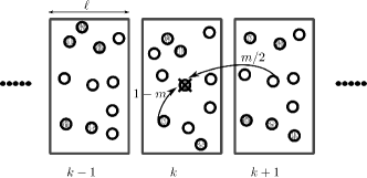
Let us consider an infinitely extended one-dimensional collection of islands and call $n_{i}$ the number of mutant individuals on island $i$. We use the vector $\mathbf{n}$ as a shorthand notation for the collection of these numbers $\mathbf{n}=\{...,n_{i},...\}$. The transition probability densities for the number of mutants on island $i$ to increase/decrease by one individual isHouchmandzadeh2011b :

$$W_{i}^{+}(\mathbf{n}) = \frac{\mu(1+s)}{N}(N-n_{i})\left[n_{i}+\frac{m}{2}n^{\prime\prime}_{i}\right]$$ (2)

$$W_{i}^{-}(\mathbf{n}) = \frac{\mu}{N}n_{i}\left[(N-n_{i})-\frac{m}{2}n^{\prime\prime}_{i}\right]$$ (3)

where $\mu$ is the death rate of individuals and

$$n^{\prime\prime}_{i}=(n_{i-1}+n_{i+1}-2n_{i}).$$ (4)

The rate of increase (2) for example is the probability density per unit of time that one wild type individual dies ($\mu(N-n_{i})$ ) multiplied by the probability that it is replaced by a mutant, either from a local parent ($(1-m)n_{i}/N$) or a neighboring parent ($(m/2N)(n_{i-1}+n_{i+1})$ ), and multiplied by the fitness of the mutant $(1+s)$. The fitness can be seen as an increase in the death rate of the wild type individuals, or a higher replacement probability/decreased death rate for the mutants. The probability $P(\mathbf{n},t)$ of observing the state $\mathbf{n}$ at time $t$ obeys the Master equation

$$\frac{dP(\mathbf{n})}{dt} = \sum_{i}\left(W_{i}^{+}(a_{i}\mathbf{n})P(a_{i}\mathbf{n})-W_{i}^{+}(\mathbf{n})P(\mathbf{n})\right)$$ (5)

$$+ \left(W_{i}^{-}(a_{i}^{\dagger}\mathbf{n})P(a_{i}^{\dagger}\mathbf{n})-W_{i}^{-}(\mathbf{n})P(\mathbf{n})\right)$$

where $a_{i}^{\dagger}\mathbf{n}$ and $a_{i}\mathbf{n}$ are shorthand notations for states $\{...,n_{i}\pm 1,...\}$. Without loss of generality (see Mathematical Details V.4), the initial condition we use throughout this article is that of an initial sharp front

$$n_{i}=N\,\,\,\mbox{if}\,\,i\leq 0;\,\,=0\,\,\mbox{otherwise}$$ (6)

II.1 Mean field approximation.

The mean field approximation for $\left\langle n_{i}\right\rangle$, the average number of individuals on island $i$, is obtained by neglecting fluctuations (i.e., by setting $\left\langle n_{i}n_{k}\right\rangle=\left\langle n_{i}\right\rangle\left\langle n_{k}\right\rangle$ )

$$\frac{d\left\langle n_{i}\right\rangle}{dt} = \left\langle W_{i}^{+}(\mathbf{n})-W_{i}^{-}(\mathbf{n})\right\rangle$$

$$= \frac{\mu m}{2}\left\langle n^{\prime\prime}_{i}\right\rangle+\frac{s\mu}{N}\left(N-\left\langle n_{i}\right\rangle\right)\left(\left\langle n_{i}\right\rangle+\frac{m}{2}\left\langle n^{\prime\prime}_{i}\right\rangle\right)$$

Taking the space continuum limit by setting $x=\ell i$, $u(x)=n_{i}/N$, we obtain the partial differential equation

$$\frac{\partial u}{\partial t}=D\left[1+s(1-u)\right]\frac{\partial^{2}u}{\partial x^{2}}+\mu su(1-u)$$ (7)

where the length $\ell$ is the spatial extension of an island and $D=\mu m\ell^{2}/2$ is the diffusion coefficient. We observe that the mean field equation of the spatial Moran model is different from the FKPP equation in the diffusion term. Fisher himself, in his original articleFisher1937 , had stressed that using a simple diffusion term is an oversimplification of basic population genetics processes. The modification of the diffusion term has important consequences both on the speed of the propagation front and on its width. The minimum speed of the propagating wave in the equation (7) is now (see Mathematical details V.3)

$$c_{min}=2\sqrt{\mu Ds(1+s)}$$ (8)

which scales as $s$ for high value of the excess fitness, in contrast to the scaling in $\sqrt{s}$ in the FKPP equation. Numerical resolutions of eq.(7) (Figure 2) show that $v_{min}$ computed above is an excellent estimator of the speed of the front.

Figure 2: The FKPP (black circle) and the spatial Moran mean field (equation 7) (red squares) are solved numerically for $\mu=1,$ $D=0.04$ and the front speed is extracted for various values of the excess relative fitness $s$. Solid curves represent the theoretical values: FKPP $c=2\sqrt{\mu Ds}$; Moran $c=2\sqrt{\mu Ds(1+s)}$. Inset : Width of the front as a function of $s$. Black circle: FKPP; red square: Moran. Solid curves represent, for FKPP (black) $B=2\sqrt{D/\mu s}$; for Moran (red) $B=2\sqrt{D(1+s)/\mu s}\,\kappa(s)$ (eq. 51).

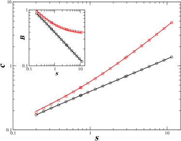
Furthermore, the width of the front does not scale as $\sqrt{D/\mu s}$ as in the case of the FKPP equation, but is well approximated by

$$2\sqrt{D(1+s)/\mu s}\,\kappa(s)$$ (9)

where $\kappa(s)$ is a small correction (see Mathematical details V.3). Specifically, for large $s$, the width converges to a constant $(15/8)\sqrt{D/\mu}$.

A phenomenological argument can be used to understand these modifications to the FKPP equation. It is well knownPanja2003 that the dynamics of a pulled front is governed by the behavior at small $u$. In these regions, the mean field equation (7) can indeed be approximated by an FKPP equation, with the effective diffusion coefficient $D_{eff}=D(1+s)$.

We observe that the spatial Moran model differs significantly from the prediction of FKPP equation at high fitness $s$. We will show below that the same is true at low fitness. This difference was first noted by Hallatschek and KorolevHallatschek2009 in their study of the SFKPP equation.

II.2 Stochastic characterization of the front.

Let us now come back to the full stochastic treatment of the propagating front. The temporal evolution of local population moments can be extracted from the Master equation (5) (see Appendix V.2):

$$\frac{d\left\langle n_{i}\right\rangle}{dt} = \left\langle W_{i}^{+}-W_{i}^{-}\right\rangle$$

$$\frac{d\left\langle n_{i}n_{j}\right\rangle}{dt} = \left\langle n_{i}\left(W_{j}^{+}-W_{j}^{-}\right)+n_{j}\left(W_{i}^{+}-W_{i}^{-}\right)\right\rangle$$

$$+ \delta_{i,j}\left\langle W_{i}^{+}+W_{i}^{-}\right\rangle.$$

The most important global quantities are the front displacement $U(t)$ and its width $B(t)$. These global quantities can be measured in terms of local populations by

$$U(t) = \frac{1}{N}\sum_{i=-\infty}^{+\infty}\left[n_{i}(t)-n_{i}(0)\right]$$ (10)

$$B(t) = \frac{1}{N^{2}}\sum_{i=-\infty}^{+\infty}n_{i}(t)\left[N-n_{i}(t)\right]$$ (11)

The width $B(t)$ weights the region where the mutant population is different from either $0$ or $N$, and in the continuous limit, can be expressed as $B=\int_{I}u(1-u)dx$ where $u(x)=n_{i}/N$. Note that these quantities are always finite, as the sums involve only a finite number of non-zero terms. We restrict this paper to the computation of the first moments of these quantities, namely $\left\langle U(t)\right\rangle$, $\mbox{Var}(U(t))$ and $\left\langle B(t)\right\rangle$, where $\left\langle\right\rangle$ stands for ensemble average. The computation of these quantities implies the computation of the second moments

$$Z_{p}(t)=\frac{1}{N^{2}}\sum_{i}\left\{\left\langle n_{i}(t)n_{i+p}(t)\right\rangle-n_{i}(0)n_{i+p}(0)\right\}$$ (12)

The width of the front is then

$$\left\langle B(t)\right\rangle=-Z_{0}(t)+\left\langle U(t)\right\rangle+B(0)$$ (13)

and the variance of its displacement is

$$V(t) = \left\langle U^{2}(t)\right\rangle-\left\langle U(t)\right\rangle^{2}$$ (14)

$$= \frac{1}{N^{2}}\sum_{i,j}\left\langle n_{i}n_{j}\right\rangle-\left\langle n_{i}\right\rangle\left\langle n_{j}\right\rangle$$

For the neutral front ($s=0$), self consistent, exact equations without any moment closure approximation can be derived directly for the global quantities. At small selection pressures $Ns\ll 1$, they can be recovered through a first order perturbation analysis.

II.3 Behavior of the neutral front $s=0$.

For a one dimensional system where mutants and wild type have the same fitness ($s=0$), we will show that the front separating these two populations can be envisioned as a well defined object that performs a Brownian motion and whose width fluctuates around an equilibrium value: $\left\langle U(t)\right\rangle=0$ and for large times, $V(t)=mt$ and $\left\langle B(t)\right\rangle=m(N-1)/2$.

To obtain the above quantities, we sum over local fluctuations

$$\frac{1}{\mu}\frac{d\left\langle n_{i}\right\rangle}{dt} = \frac{m}{2}\left\langle n^{\prime\prime}_{i}\right\rangle$$

$$\frac{1}{\mu}\frac{d\left\langle n_{i}n_{j}\right\rangle}{dt} = \frac{m}{2}\left(\left\langle n^{\prime\prime}_{i}n_{j}\right\rangle+\left\langle n_{i}n^{\prime\prime}_{j}\right\rangle\right)$$

$$+ \delta_{i,j}\left\{\frac{2}{N}\left\langle n_{i}(N-n_{i})\right\rangle+\frac{m}{2}\left\langle n^{\prime\prime}_{i}\right\rangle-\frac{m}{N}\left\langle n_{i}n^{\prime\prime}_{i}\right\rangle\right\}$$

There are different contributions to $d\left\langle n_{i}n_{i}\right\rangle/dt$ : one is the local demographic noise $2\left\langle n_{i}(N-n_{i})\right\rangle/N$, which appears in the SFKPP equation ; the other term, $m\left\langle n_{i}n^{\prime\prime}_{i}\right\rangle/N$, is the demographic noise due to adjacent cells and cannot a priori be neglected. In the extreme case where $N=1$ and therefore $m=1$, the local demographic noise is exactly zero, but the stochasticity of the system remains the same, as we will see below.

From now on, we will measure time in generation time units, i.e., set $t\leftarrow\mu t$. By summing over the first moments, we find trivially that the mean front position stays at its initial value

$$\frac{d}{dt}\left\langle U(t)\right\rangle=\frac{m}{2}\sum_{i}\left\langle n^{\prime\prime}_{i}\right\rangle=0$$

The second moments on the other hand obey a set of linear differential equations

$$\frac{1}{m}\frac{dZ_{0}}{dt} = -2(1+\alpha)Z_{0}+2(1-\beta)Z_{1}+(1-\beta)C_{0}$$ (15)

$$\frac{1}{m}\frac{dZ_{p}}{dt} = -2Z_{p}+Z_{p+1}+Z_{p-1}+C_{p}\,\,\,\,\,\,p>0$$ (16)

where $\alpha=(1-m)/(Nm)$, $\beta=1/N$ and the coefficients $C_{p}$ depend on the initial conditions :

$$C_{p}=\frac{1}{N^{2}}\sum_{i}n_{i}(0)n^{\prime\prime}_{p+i}(0)$$

The parameters $\alpha$ and $\beta$ measure the relative contribution to the demographic noise of local versus adjacent cells . The parameter $\beta$ can be neglected with respect to $\alpha$ only in the limit of small migration probability $m\ll 1$.

For an initially sharp front (eq. 6), $C_{p}=-\delta_{p,0}$. We stress that we can assume this condition without loss of generality (see Appendix V.4)

The above system (15,16) can be solvedHouchmandzadeh2003 exactly. In the Laplace space where $\hat{Z}_{p}(\omega)=\int_{\mathbb{R}^{+}}\exp(-\omega t)Z_{p}(t)dt$, the solution is particularly simple,

$$\hat{Z}_{p}(\omega)=\frac{(1-\beta)C_{0}}{\omega}\frac{z}{z^{2}+2\alpha z+2\beta-1}\frac{1}{z^{p}}$$

where $\omega=(z+1/z)-2$. By taking the inverse Laplace transform the exact solution of $Z_{p}(t)$ can be found as a combination of modified Bessel functionsHouchmandzadeh2003 . In this article, we are mostly concerned with the large time limit, which can be deduced from the expansion of $\hat{Z}_{p}(\omega)$ around $\omega=0$ :

$$\hat{Z}_{p}(\omega) = -\frac{m(N-1)}{2}\left(\frac{1}{\omega}+\frac{p-K}{\sqrt{\omega}}\right)+\mathcal{O}(1)$$

$$Z_{p}(t) = -\frac{m(N-1)}{2}\left(1+\frac{p-K}{\sqrt{\pi mt}}\right)+o(t^{-1/2})$$ (17)

where $K=m(N-1)+2$. The above approximation is valid for $t\gg p^{2}$; a uniform large time approximation for all $p$ can also be found in terms of combinations of erf functionsHouchmandzadeh2003 , but is not needed here.

As $B(0)=0$ and $\left\langle U(t)\right\rangle=0$, eq.(13) implies that

$$\left\langle B(t)\right\rangle=-Z_{0}(t).$$

The front therefore reaches a finite width

$$B_{\mbox{eq}}=m(N-1)/2$$ (18)

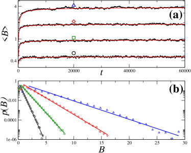
and the equilibrium value is reached as $1/\sqrt{mt}$. Figure 3a shows the perfect agreement of these results with numerical simulations. The above equilibrium value of the width is also in agreement with the value found from the SFKPP equationHallatschek2009 $4Db^{-1}$ if the amplitude of the noise term is interpreted as $b=4\mu\ell/N$. As noted by Hallatschek and KorolevHallatschek2009 , genetic drift alone can maintain a finite front width at $s=0$ in one dimension. Moreover, numerical simulations of the discrete model show that the width distribution probability of the front has an exponential tail (figure 3b)

Figure 3: Front’s width (eq. 11) computed from numerical simulations of the master equation (5) by a Gillespie algorithm comprising $M=2000$ sites (islands) for four sets of parameters $(N,m)$: Black circles $(20,0.05)$ ($B_{\mbox{eq}}=0.475$); green squares $(40,0.05)$ ($B_{\mbox{eq}}=0.975$); red diamonds $(20,0.2)$ ($B_{\mbox{eq}}=1.9$); blue triangles $(40,0.2)$ ($B_{\mbox{eq}}=3.9$). (a) average front $\left\langle B(t)\right\rangle$ computed over $10^{3}$ stochastically generated $B(t)$, for $t\in[0,10^{5}]$. Dotted black curves : numerical simulations ; solid red curves : theoretical prediction $B(t)=-Z_{0}(t)$ (eq17). (b) probability distribution of the width $B$ after equilibrium has been reached ($t\in[1,100]\times 10^{5}$, sampling time$10^{2}$ ) for the same parameters as in panel a. Symbols: numerical simulations ; solid curves : exponential fits of the data $p(B)=A\,\exp(-aB)$ after the peak of the distribution has been reached

Note that the width $B$ defined above as

$$\left\langle B\right\rangle=\sum_{i}\left\langle b_{i}\right\rangle=\frac{1}{N^{2}}\sum_{i}\left\langle n_{i}(N-n_{i})\right\rangle$$

weights the regions with populations $0<n_{i}<N$, but contains no information about their spatial distribution. A spatially wide front composed for example of alternating $n=0$ and $n=N$ islands will have $B=0$.

The shape of the front can be characterized more precisely by using the moving frame of the front as the reference frame and computing the mean relative mutant number $\nu_{i}$ and their weight $\beta_{i}$ in this frame

$$\nu_{i} = \frac{1}{N}\left\langle n_{i+[U]}\right\rangle$$ (19)

$$\beta_{i} = \nu_{i}(1-\nu_{i})$$ (20)

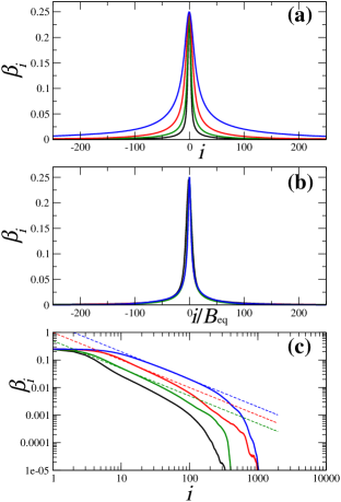
where $[U]$ is the integer part of the front displacement given by the relation (10). These quantities are difficult analytically but are readily computed by numerical simulation, as shown in Figure 4. As it can be observed, the mean front shape $\beta_{i}$ , which is a function of $N$ and $m$ (Figure 4a) is spatially extended and decreases slowly as a function of $i$, the distance to the center of the front (Fig. 4c). The width $B_{\mbox{eq}}$ computed above remains however a good indicator of the mean front shape, and all $\beta_{i}$ curves can be superimposed when the normalized index $i/B_{\mbox{eq}}$ is used(Fig. 4b).

Figure 4: Mean front shape $\beta_{i}$ (eq. 20) as a function of distance to the center of the front $i$, in the moving reference frame. Numerical simulations schemes are the same as in figure 3, with $M=6000$. In each sampled stochastic realization, the displacement is computed from the relation (10) and the mutant population numbers in each site $i$ in a window of 1000-2000 sites around this position are recorded. The mean front shape $\nu_{i}$ (eq.19) is computed on approximately $10^{7}$ samples. (a) $\beta_{i}$ as a function of $i$ for various $(N,m$) parameters : $(20,0.05)$ black, $(40,0.05)$ green, $(20,0.2)$ red, (40,0.2) blue. (b) Same as in panel (a), but the $x$ axis for each curved is normalized by the corresponding equilibrium width $B_{\mbox{eq}}=(N-1)m/2$. (c) The long tail of the front $\beta_{i}$ (solid curves), where the parameters are the same as in panel (a). The dashed lines represent the function $y=B_{\mbox{eq}}/2i$ as visual guides.

The variance of the position of the front $V(t)=\left\langle U^{2}(t)\right\rangle-\left\langle U(t)\right\rangle^{2}$ can be extracted by similar methods from equation (14) :

$$\frac{dV}{dt} = \frac{2}{N^{3}}\sum_{i}\left\{\left\langle n_{i}(N-n_{i})\right\rangle-\frac{m}{2}\left\langle n_{i}n^{\prime\prime}_{i}\right\rangle\right\}$$

$$= \frac{2}{N}\left\{\left\langle B(t)\right\rangle-m\left(Z_{1}(t)-Z_{0}(t)\right)-\frac{m}{2}C_{0}\right\}.$$

As $Z_{p}(t)$ can be computed exactly, the temporal evolution of the variance can also be computed exactly. The result is particularly simple for large times $t\gg 1$

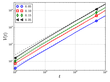
$$V(t)=mt+\mathcal{O}(\sqrt{mt})$$ (21)

The surprising result is that for large times, the diffusion of the front is independent of its width. The figure 5 shows the agreement of this expression with numerical solutions.

Figure 5: Solid curves: Variance of the position of the neutral front as a function of time, computed from numerical simulations of the master equation (5) by a Gillespie algorithm, for various values of the migration parameter $m$=0.05,0.1,0.15,0.25 and $N=10$. Dashed lines: the theoretical values of $V(t)=mt$ (eq. 21) for corresponding $m$. The numerical simulations comprised $M=2000$ sites and the variance was computed over $6.4\times 10^{3}$ stochastically generated $U(t)$, for $t\in[0,10^{5}]$.

II.4 Behavior of the front at small $s$.

For a non-zero excess relative fitness, the moment closure does not hold and the front characteristics can no longer be derived exactly. It is however possible to derive the front speed to the first order of the perturbation $s$.

For $s>0$ the position of the front is given by

$$\frac{d\left\langle U\right\rangle}{dt} = \frac{1}{N}\sum_{i}\left\langle W_{i}^{+}(\mathbf{n})-W_{i}^{-}(\mathbf{n})\right\rangle$$

$$= s\left\{B(t)-m\left(Z_{1}(t)-Z_{0}(t)\right)-\frac{m}{2}C_{0}\right\}$$

At small selection pressures $Ns\ll 1$, on expanding the above expression to the first order of perturbation, we find, in the limit of large time

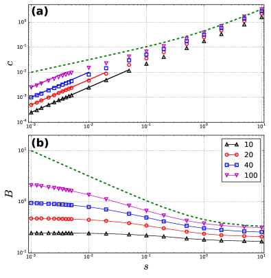
$$\frac{d\left\langle U\right\rangle}{dt}=\frac{mNs}{2}+{\cal O}(1/\sqrt{t})$$ (22)

Note that at small $s$, the front speed scales as the selection pressure $Ns$. Even for $N=1$ when the front width $B_{eq}=0$, the front acquires a non-zero speed (figure 6).

The above computation of the position of the front at $s>0$, which is a first order moment, requires the knowledge of second order moments $Z_{i}$ at $s=0$. The same line of argument shows that computing the variance of the position and width of the front for $s>0$ , which are second order moments, necessitates the computation of third order statistical quantities. Even though computation of higher momenta is theoretically possible in the neutral case $s=0$, their effective computation remains extremely tedious.

Figure 6 shows the result of stochastic based numerical simulations for a wide range of $s$ and the agreement with expression (22) at small selection pressure. It can be observed that the mean field approximation becomes correct only at very high excess relative fitness $s$ and local population size $N$. Fluctuations modify significantly the prediction of the FKPP model.

Figure 6: Speed $c$ (panel (a) ) and width $B$ (panel B) of the front as a function of excess relative fitness $s$ for $m=0.05$ and $N=10$, $20$,$40$, and $100$. Solid lines in panel (a) represent the first order theoretical expression $c=Nms/2$ for $Ns\lesssim 0.5$. Dashed green lines represent the mean field values $c_{\mbox{m.f}}=\sqrt{2ms(s+1)}$ and $B_{\mbox{m.f}}=\sqrt{2m(s+1)/s}$.

III Microscopic model and general migration kernel.

In the SFKPP description of the mutant wave (eq.1) the diffusion coefficient $D$ and the amplitude of the noise $b$ are considered independent parameters. The same is true for the island model of the preceding section where the population size of the island $N$ and the migration probability $m$ between neighboring islands were considered independent. However, at the individual level of evolution, both migration and genetic drift are the result of the same phenomenon of individuals replacing each other. These two parameters must therefore be linked through an Einstein-like relation and cannot be independent.

There is a level of arbitrariness in the island model in the manner in which individuals are grouped together and deme size $N$ is chosen. As the amount of fluctuations is critically controlled by $N$, the grouping process is crucial. This arbitrariness also impacts on the migration probability. The very existence of a unique migration rate between nearest neighbor islands can be brought into question. Consider for example the low migration limit ($m\ll 1$) of the island model: two individuals physically far apart from each other but grouped into the same island will have a higher probability of replacing each other than two close individuals belonging to neighboring islands.

Figure 7: Neutral spatial Moran model with general migration kernel. (a) Individuals are uniformly distributed in space ; when an individual at site $i$ dies, it is replaced by the progeny of its $k-$th neighbor with probability $m(k)$. (b) Individuals are grouped into demes of population size $N^{\star}$. In the classical scheme of SFKPP (figure 1), the detailed migration kernel $m(k)$ is replaced by a single number $m^{\star}$ of migration between neighboring demes.

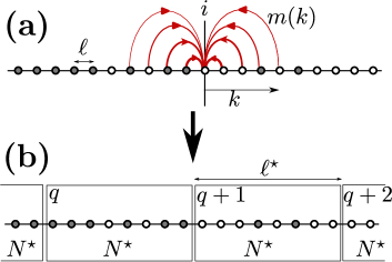
A more rigorous approach to this problem would be to consider a “microscopic” model where individuals are uniformly distributed in space and not arbitrarily grouped into demes/islands. In this microscopic model, migration/replacement is not restricted to nearest neighbors (figure 7a): when an individual dies at site $i$, it has a probability $m_{i}^{j}$ of being replaced by the progeny of an individual at site $j$. Solving exactly this strictly individual model then leads us to choose the effective population size of each deme, which is used in the stepping stone approach (figure 7b) and derive the exact relation between the diffusion coefficient and the noise amplitude, both of which are a function of the dispersal kernel $m_{i}^{j}$.

In this evolutionary graph approach, each site contains exactly one individual (either wild type or mutant) $n_{i}=0,1$ ; the transition probability densities for the number of mutants on site $i$ to increase/decrease by one individual is a simple generalization of equations (2,3) . Thus:

$$W_{i}^{+}(\mathbf{n}) = (1+s)\mu(1-n_{i})\sum_{j}m_{i}^{j}n_{j}$$ (23)

$$W_{i}^{-}(\mathbf{n}) = \mu n_{i}\sum_{j}m_{i}^{j}(1-n_{j})$$ (24)

where $m_{i}^{j}$ is the probability that the progeny of an individual at site $j$ replaces an individual at site $i$. In the literature of plants, the migration probability $m_{i}^{j}$ is known as the dispersal kernel and can be measured precisely in the fieldNathan2000 . In the following, we will consider dispersal kernels that depend only on the distance between two sites, $i.e.$, $m_{i}^{j}=m(|j-i|)$.

III.1 Mean field approximation.

Following the same steps as in subsection II.1, it is straightforward to deduce the mean field approximation of the corresponding master equation. For a migration probability that depends only on the distance between two sites, the mean field approximation is exactly the same as expression (7), where $\ell$ here is the inter-individual distance (lattice size), $\mu$ the death rate and the diffusion coefficient

$$D=\frac{\mu\ell^{2}}{2}\sum_{k}k^{2}m(k)$$ (25)

is given in terms of mean dispersal distance.

From now on and to avoid confusion, we will refer to all quantities derived in the island approximation (the macroscopic view) of section II by the super script ^⋆ . The diffusion coefficient of the mean field approximation derived in subsection II.1 (relation 7), for example, is

$$D^{\star}=\frac{\mu\ell^{\star 2}}{2}m^{\star}$$ (26)

For a 1d system, the patch extension $\ell^{\star}=N^{\star}\ell$ (figure 7b) ; comparing expression (25) and (26) therefore leads to

$$N^{\star 2}m^{\star}=\sum_{k}k^{2}m(k)$$ (27)

We observe here that the deme size $N^{\star}$ and the migration probability between demes $m^{\star}$ are indeed linked through equation (27).

III.2 Stochastic characterization of the neutral front at $s=0$.

The relation (27) is not sufficient to determine the effective population size $N^{\star}$ of islands. To address this issue, we need to solve exactly the full stochastic model. We restrict the computation here to the neutral case $s=0$, the derivations for $s\neq 0$ following precisely the steps developed previously.

The computational approach is similar to subsection II.2. As before, the displacement of the front is defined as

$$U(t)=\sum_{i=-\infty}^{+\infty}\left[n_{i}(t)-n_{i}(0)\right]$$ (28)

and

$$\frac{d}{dt}\left\langle U(t)\right\rangle=\sum_{i}\left\langle W_{i}^{+}(\mathbf{n})-W_{i}^{-}(\mathbf{n})\right\rangle$$

Therefore, for the neutral front $s=0$, $d_{t}\left\langle U\right\rangle=0$ and $\left\langle U(t)\right\rangle=0$.

The second order moments are also defined as before

$$Z_{p}(t)=\sum_{i}\left\langle n_{i}(t)n_{i+p}(t)\right\rangle-n_{i}(0)n_{i+p}(0)$$ (29)

and we note that $Z_{p}=Z_{-p}.$ The equations governing $Z_{p}$ for the rescaled time $t\leftarrow\mu t$ are

$$\frac{d}{dt}Z_{0} = -2Z_{0}$$ (30)

$$\frac{d}{dt}Z_{p} = 2\sum_{k=-\infty}^{\infty}m(k)\left(Z_{p+k}-Z_{p}\right)+C_{p}\,\,\,\,p\neq 0$$ (31)

where the $C_{p}$ are defined by the initial condition

$$C_{p}=2\sum_{k}m(k)\sum_{i}n_{i}(0)\left(n_{i+p+k}(0)-n_{i+p}(0)\right)$$

Note that equation (30) implies that $Z_{0}(t)=0.$ This is due to the fact that $n_{i}^{2}=n_{i}$ and therefore $Z_{0}(t)=\left\langle U(t)\right\rangle$.

For an initially sharp front

$$n_{i}=1\,\,\,\mbox{if}\,\,i\leq 0;\,\,=0\,\,\mbox{otherwise}$$ (32)

which will be used here,

$$C_{p}=2\sum_{k>\left|p\right|}m(k)\left(\left|p\right|-k\right)$$ (33)

For simplicity, we further restrict the solution of equations (30-31) to the generic geometric dispersal kernel

$$m(k)=(1-\delta_{k,0})\frac{1-\lambda}{2\lambda}\lambda^{\left|k\right|}$$ (34)

where the parameter $\lambda$ controls the dispersal length $\kappa$:

$$\kappa^{2}=2\sum_{k>0}k^{2}m(k)=\frac{1+\lambda}{(1-\lambda)^{2}}$$ (35)

The case $N^{\star}=1$, $m^{\star}=1$ of the preceding section is obtained when $\lambda\rightarrow 0$. Note that in the framework of the Moran model used here, a dead individual cannot replace itself, hence $m(0)=0$. Moreover, for the geometric dispersal kernel, relation (33) becomes

$$C_{p}=\frac{-1}{1-\lambda}\lambda^{\left|p\right|}$$

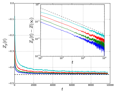
It is straightforward to check that again all $Z_{p}$ converge as $\propto 1/\sqrt{t}$ to the same value

$$Z_{p}(\infty)=-\frac{\lambda}{(1-\lambda)^{2}}=\theta^{2}-\kappa^{2}$$ (36)

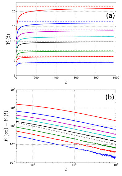
where $\kappa^{2}$ is defined in (35) and $\theta=2\sum_{k>0}k\,m(k)$$=1/(1-\lambda)$. We observe that the stationary value of $-Z_{p}$ is given by a quantity similar to the variance of the dispersal kernel. Figure 8 shows the agreement between these results and individual based numerical simulation of the same system.

Figure 8: Numerical simulation of the second moment $Z_{p}$ (eq. 29) in the neutral Moran model with geometric seed dispersal kernel (eq. 34) for $p=1,2,4,8$. (Inset) Same data but convergence to the limiting value $Z(\infty)$ is shown ; the gray dashed line is $\propto 1/\sqrt{t}$. Time is measured in units of generation time ($1/\mu)$. For the numerical simulation, a lattice of 4096 individuals is used and the result is averaged over $8\times 10^{5}$ trials.

The width of the front can no longer be measured as in relation (11) by $B=\sum_{i}n_{i}(1-n_{i})$ which is always $0$. Other analog metrics such as

$$Y_{p}=\sum_{i}(n_{i}-n_{i+p})^{2}$$ (37)

can be used to characterize the front. It is straightforward to show that

$$Y_{p}=p-2Z_{p}$$ (38)

Figure 9 shows the excellent agreement between the theoretical results and the numerical simulations.

Figure 9: (a) Numerical simulation of the front width $Y_{1}(t)$ (eq. 37) in the neutral Moran model with geometric seed dispersal kernel (eq. 34) for increasing value of $\lambda=$0.25,0.33,0.4,0.5,0.55,0.6,0.66 and 0.75. (b) Same data but convergence to the limiting value $Y_{1}(\infty)$ is shown ; the gray dashed line is $\propto 1/\sqrt{t}$. Time is measured in units of generation time ($1/\mu)$. The numerical simulation parameters are identical to figure 8.

The variance of the front displacement $V=\left\langle U^{2}\right\rangle-\left\langle U\right\rangle^{2}$ can be computed by methods analogous to the previous section:

$$\frac{dV}{dt} = \sum_{i}\left(W_{i}^{+}+W_{i}^{-}\right)$$

$$= -2\sum_{k}m(k)Z_{k}-C_{0}$$

where the $W_{i}^{\pm}$ are the transition rates (23,24) and $C_{0}$ is defined by relation 33). For the geometric kernel $m(k)$ (eq. 34), using the long term solution (36) leads to

$$V(t)=\kappa^{2}t+{\cal O}(\sqrt{t})$$ (39)

III.3 Grouping into islands.

We now group individuals virtually into islands of size $N^{\star}$ and establish the condition under which the results obtained by the SFKPP/islands model are valid.

A patch of population size $N^{\star}$ is a virtual packing of individuals into a deme, which we refer to by its index $q$ (Figure 7b). The number of mutants in patch $q$ is

$$n_{q}^{\star}=\sum_{a_{q}}^{b_{q}}n_{i}$$ (40)

where $b_{q}=a_{q}+N^{\star}-1$ and $a_{q+1}=b_{q}+1$. Note that we have $N^{\star}$ possible choices for grouping individuals, as we can set $a_{q}=N^{\star}q+r$, where $r=0$, 1, …,$N^{\star}-1$. We define the displacement and the width of the (macroscopic) front as in subsection II.2 (definitions 10,11)

$$U^{\star}(t) = \frac{1}{N^{\star}}\sum_{q=-\infty}^{+\infty}\left[n_{q}^{\star}(t)-n_{q}^{\star}(0)\right]$$ (41)

$$B^{\star}(t) = \frac{1}{N^{\star 2}}\sum_{q=-\infty}^{+\infty}n_{q}^{\star}(t)\left[N^{\star}-n_{q}^{\star}(t)\right]$$ (42)

We compute the statistical properties of these quantities by taking into account the detailed migration kernel (subsection III.2) and compare them to the results obtained in subsection II.2 where migrations were approximated by a single migration probability $m^{\star}$ between neighboring demes.

The macroscopic displacement $U^{\star}$ (relation 41) is easily related to the microscopic displacement $U$ (relation 28) :

$$U^{\star} = \frac{1}{N^{\star}}\sum_{q=-\infty}^{+\infty}\sum_{a_{q}}^{b_{q}}\left[n_{i}(t)-n_{i}(0)\right]$$

$$= \frac{1}{N^{\star}}\sum_{i=-\infty}^{\infty}\left[n_{i}(t)-n_{i}(0)\right]$$

$$= \frac{1}{N^{\star}}U$$

and therefore $V^{\star}=\text{Var}(U^{\star})=\text{Var}(U)/N^{\star 2}$. The variance of the microscopic displacement $V$ is given by relation (39), and hence, for long times,

$$V^{*}=\frac{\kappa^{2}}{N^{\star 2}}t$$ (43)

Comparing this expression to the relation $V^{\star}=m^{\star}t$ of the island model (section II) where $m^{\star}$ is the migration probability between demes, we see that we must have

$$m^{\star}=\kappa^{2}/N^{\star 2}$$ (44)

The above relation is a confirmation of relation (27), which we obtained by a mean field approximation. We can also compute, at small selection pressure $Ns$, the speed of the front that we find to be $c=s\kappa^{2}/2$. Comparing this result to the speed $c^{\star}=c/N^{\star}=sN^{\star}m^{\star}/2$ (eq. 22) of the island model leads again to the same relation between $m^{\star}$ and $N^{\star}$ as relation (44).

The macroscopic width of the front (relation 42) can also be computed in terms of microscopic quantities (see Appendix V.5)

$$B^{\star}=\frac{1}{N^{\star 3}}\sum_{p=1}^{N-1}(N^{\star}-p)Y_{p}$$

where $Y_{p}$ are the microscopic front width (defined by relation 37). For large times, relations (38) and (36) lead to

$$B^{\star}=\frac{N^{\star}-1}{N^{\star 2}}\left[\kappa^{2}-\theta^{2}+\frac{1}{6}(N^{\star}+1)\right]$$ (45)

The above relation is in perfect agreement with numerical simulations. Comparing the above relation to the width of the front $B^{\star}=m^{\star}(N^{\star}-1)/2$ of the island model (relation 18) and using relation (44) for $m^{\star}$, we find that we must have

$$N^{\star}=3\theta-1$$ (46)

The above result determines the effective population size in terms of the dispersal kernel. More precisely,

$$N^{\star} = \frac{2+\lambda}{1-\lambda}$$

$$m^{*} = \frac{1+\lambda}{(2+\lambda)^{2}}$$

We note that $m^{\star}$ is weakly dependent on $\lambda$ over its whole range of variation [0, 1], whereas $N^{\star}$ diverges as the dispersion characteristic length when $\lambda\rightarrow 1$.

IV Discussion and conclusion.

In this article, we have used the formalism of the spatial Moran model to study the propagation of mutants in a one dimensional geographically extended population. The propagation of the mutant wave has usually been studied in the framework of the SFKPP equation (1). The SFKPP equation however is a phenomenological approach and its derivation from the fundamental models of population genetics such as Wright-Fisher or Moran is not obvious. The deterministic Fisher equation for the dynamics of the proportion $u(t)$ of a mutant in a non-structured population is $d_{t}u=su(1-u)$. For geographically structured populations, it seemed naturalFisher1937 to add a spatial diffusion term and generalize simply this equation to $\partial_{t}u=D\Delta u+su(1-u)$, where $u(x,t)$ is the local proportion of the mutant. On the other hand, since the time of Fisher and Wright, it was obvious that genetic drift is an important factor at small selection pressure. For large non-structured ($d=0)$ populations, Kimura tackled this problem by using a Fokker-Planck approximation of the Master equations governing the WF or Moran models. The stochastic differential equation associated with the Kimura equation is $d_{t}u=su(1-u)+\sqrt{u(1-u)/N}\eta(t)$. It then seemed natural to unite the two approaches and propose the SFKPP equation (1).

We see here that many assumptions were made in this process : (i) the form of the diffusion term may be different ; (ii) $u(x,t)$ is a local relative density and the noise term of SFKPP would be a good approximation only if the number of individuals in each patch where $u$ has been computed is large enough ; (iii) the noise term $\sqrt{u(1-u)/N}$ itself was obtained for a non-structured population and it is far from obvious that it should be the same for an extended population and not involve the spatial derivative of $u$.

The individual based approached that we develop in this article is intended to overcome these problems and to ground the SFKPP approach on a firmer basis. Using an explicit spatial island model, we have shown first that the diffusion term is indeed different from the FKPP equation (relation 7) and this difference has important consequences on the speed and width of the front for large selection pressures (relation 8,9).

For small selection pressures, we derive the parameters of the front (speed, diffusion coefficient and width) without any assumption on the size of the local population and without neglecting the non-local noise. These results are in agreement with the predictions of SFKPP equation at small selection pressure as developed by Hallatschek2011 .

Finally, by taking into account the explicit migration kernel, we establish the relation between the amplitude of the diffusion and that of the noise ; this approach also allows us to define the effective size of the local population $N$, which is the crucial parameter controlling the noise as a function of the dispersal length.

Individual based models have the same level of complexity as their equivalent stochastic differential equation approach. We believe that the formalism developed in this article is a step forward in the search for a better understanding of natural populations and the dynamics of mutant waves.

V Mathematical details.

V.1 The noise term in SFKPP

The argument for the phenomenological noise term used by Doering et al. can be rephrased as follows in the framework of population genetics. For a non-structured population (a population at $d=0)$, in an ecosystem with carrying capacity of $N$ individuals formed of wild type individuals with fitness $1$ and mutants with fitness $1+s$, the transition rates for the one-step Moran process is Houchmandzadeh2010

$$W(n\rightarrow m)=\delta_{|m-n|,1}\frac{\mu}{N}(N-n)n(1+\delta_{m-n,1}s)$$

where $n$ is the number of mutants. The probability $P(n,t)$ of observing $n$ mutants at time $t$ is governed by the Master equation associated with these rates

$$\frac{\partial P(n,t)}{\partial t}=\sum_{m}W(m\rightarrow n)P(m,t)-W(n\rightarrow m)P(n,t)$$

For a large ecosystem ($N\gg 1$) at small selection pressure $(Ns\ll 1$), the above Master equation can be approximated by a Fokker-Plank equation called the Kimura equationKimura1962 ; Ewens2004 ; Houchmandzadeh2010

$$\frac{\partial P(u,t)}{\partial t}=-s\frac{\partial\left[u(1-u)P\right]}{\partial u}+\frac{1}{N}\frac{\partial^{2}\left[u(1-u)P\right]}{\partial u^{2}}$$

where $u=n/N$ and time is measured in units of $1/\mu$. The above diffusion equation is equivalent to a stochastic differential equation for the density $u$Gardiner2004 :

$$\frac{du}{dt}=su(1-u)+\sqrt{u(1-u)/N}\eta(x,t)$$ (47)

The origin of the noise is the genetic drift due to the size of the system.

For a spatially extended system, the Doering et al. phenomenological approach to derive the SFKPP consists in adding a (spatial) diffusion term $D\nabla^{2}u$ to the stochastic equation 47, but conserving the same local noise term, and neglecting fluctuations from adjacent cells.

V.2 Moment computation algebra.

The rules of moment computations are fairly standard (see for example Pechenik1999 ), but we give them here for self-consistency. Various moments can be extracted directly from the Master Equation

$$\frac{\partial P(\mathbf{n},t)}{\partial t} = \sum_{k}\left\{W^{+}(a_{k}\mathbf{n})P(a_{k}\mathbf{n})-W^{+}(\mathbf{n})P(\mathbf{n})\right\}$$ (48)

$$+ \sum_{k}\left\{W^{-}(a_{k}^{\dagger}\mathbf{n})P(a_{k}^{\dagger}\mathbf{n})-W^{-}(\mathbf{n})P(\mathbf{n})\right\}$$

by multiplying it by some operator and then making the change of variable $\mathbf{n}\rightarrow a_{k}\mathbf{n}$ or $a_{k}^{\dagger}\mathbf{n}$. Consider for example

$$\frac{d\left\langle n_{i}n_{j}\right\rangle}{dt}=\frac{\partial}{\partial t}\sum_{\left\{\mathbf{n}\right\}}n_{i}n_{j}P(\mathbf{n},t)$$

After replacing $\partial_{t}P$ by its value from equation 48, the first term on the r.h.s. of the above equation reads:

$$I_{1}=\sum_{\mathbf{n}}\sum_{k}n_{i}n_{j}W_{k}^{+}(a_{k}\mathbf{n})P(a_{k}\mathbf{n})-(...)$$

Changing the variable $\mathbf{n}\rightarrow a_{k}^{\dagger}\mathbf{n}$ implies $n_{i}\rightarrow n_{i}+\delta_{i,k}$ and $n_{j}\rightarrow n_{j}+\delta_{j,k}$and

$$I_{1} = \sum_{\mathbf{n}}\sum_{k}\left(n_{i}+\delta_{i,k}\right)\left(n_{j}+\delta_{j,k}\right)W_{k}^{+}(\mathbf{n})P(\mathbf{n})-(...)$$

$$= \left\langle n_{i}W_{j}^{+}+n_{j}W_{i}^{+}+\delta_{i,j}W_{i}^{+}\right\rangle$$

Computing now the second term and grouping all the terms, we get

$$\frac{d\left\langle n_{i}n_{j}\right\rangle}{dt}=\left\langle n_{i}\left(W_{j}^{+}-W_{j}^{-}\right)\right\rangle+\left\langle n_{j}\left(W_{i}^{+}-W_{i}^{-}\right)\right\rangle+\delta_{i,j}\left\langle W_{i}^{+}+W_{i}^{-}\right\rangle$$

For the neutral case $s=0$ we have

$$W_{i}^{+}-W_{i}^{-}=\frac{m}{2}n^{\prime\prime}_{i}$$

and

$$W_{i}^{+}+W_{i}^{-}=\frac{2}{N}n_{i}(N-n_{i})+\frac{m}{2}n^{\prime\prime}_{i}-\frac{m}{N}n_{i}n^{\prime\prime}_{i}$$

So finally

$$\frac{d\left\langle n_{i}n_{j}\right\rangle}{dt} = \frac{m}{2}\left\langle n_{i}n^{\prime\prime}_{j}+n_{j}n^{\prime\prime}_{i}\right\rangle$$

$$+ \delta_{i,j}\left\{\frac{2}{N}\left\langle n_{i}(N-n_{i})\right\rangle+\frac{m}{2}\left\langle n^{\prime\prime}_{i}\right\rangle-\frac{m}{N}\left\langle n_{i}n^{\prime\prime}_{i}\right\rangle\right\}$$

V.3 Front speed and width in the mean field approximation.

The minimum speed of propagating front of the equation

$$\frac{\partial u}{\partial t}=D\left[1+s(1-u)\right]\frac{\partial^{2}u}{\partial x^{2}}+\mu su(1-u)$$ (49)

is obtained by following the original FisherFisher1937 approach. For a propagating front, on setting $\partial_{t}u=-v\partial_{x}u$ and then setting $g=-du/dx$, we get the equation for $g(u)$ :

$$D\left[1+s(1-u)\right]g\frac{dg}{du}-vg+\mu su(1-u)=0.$$ (50)

Setting $p=dg/du|_{u=0}$ as the slope of the curve at the origin $u=0$, the equation for $p$ is

$$D(1+s)p^{2}-vp+\mu s=0$$

which has a solution only for

$$v\geq v_{min}=2\sqrt{\mu Ds(1+s)}$$

The width $B=\int_{\mathbb{R}}u(1-u)dx$ of the front can be computed following the same approach. Setting $v=\partial_{t}\int_{\mathbb{R}}udx$, exchanging the derivation on $t$ and integration on $x$, and performing integration by parts on the propagating front, we get

$$v = \mu sB+Ds\int_{\mathbb{R}}\left(\frac{du}{dx}\right)^{2}dx$$

$$= \mu sB+Ds\int_{0}^{1}gdu$$

The shape of the front $g(u)$ is not known. However, $g(u)$ is a smooth function, $g(0)=g(1)=0$ and its slope at both ends, $p=dg/du|_{u=0}$ and $q=dg/du|_{u=1}$ are known and determined from equation (50). Approximating then $g(u)$ by a third order polynomial that respects these constraints

$$g(u)=u(1-u)(p-(p+q)u)$$

leads to:

$$B=2\sqrt{\frac{D(1+s)}{\mu s}}\kappa(s)$$ (51)

where

$$\kappa(s) = 1-\frac{s}{24(1+s)}\left(\left(\sqrt{\frac{2+s}{1+s}}-1\right)(s+1)+1\right)$$

$$= \frac{15}{16}+\frac{13}{192s}+{\cal O}(s^{-2})\,\,\,\,\mbox{for}\,\,s\gg 1$$

V.4 Choice of initial conditions.

The definition of various moments we use in this article such as relations (10-12) ensures that the infinite sums over sites contain only a finite number of non-zero terms; it avoids the problem of spurious effects due to manipulation of divergent series. However, the initial front may not need to be sharp, but only finite.

Consider the discrete function

$$f_{i}=N\,\,\,\mbox{if}\,\,i\leq 0;\,\,=0\,\,\mbox{otherwise}$$

where the position $0$ corresponds the to middle of the initial front. We can redefine the moments as

$$U = \sum_{i}n_{i}(t)-f_{i}$$

$$Z_{p} = \frac{1}{N^{2}}\sum_{i}\left\{\left\langle n_{i}(t)n_{i+p}(t)\right\rangle-f_{i}f_{i+p}\right\}$$

The differential equations we derived throughout this article remain invariant under this definition of the moments, the only difference being that the initial values of these moments are non-zero.

V.5 Relation between microscopic and macroscopic front width.

By definition,

$$N^{\star 2}B^{\star} = \sum_{q}n_{q}^{\star}(N^{\star}-n_{q}^{\star})$$

$$= \sum_{q}\sum_{i,j=a_{q}}^{b_{q}}n_{i}(1-n_{j})$$

$$= \sum_{q}\left\{\sum_{i=a_{q}}^{b_{q}}n_{i}(1-n_{i})+\sum_{i=a_{q}}^{b_{q}-1}\sum_{j=i+1}^{b_{q}}(n_{i}+n_{j}-2n_{i}n_{j})\right\}$$

where $n^{\star}$is defined by relation (40), $b_{q}=a_{q}+N^{\star}-1$ and $a_{q+1}=b_{q}+1$. Note that we have $N^{\star}$ possible choices for grouping individuals, as we can set $a_{q}=N^{\star}q+r$, where $r=0$, 1, …,$N^{\star}-1$. As $n_{i}=0,1,$ the first term in the above sum is zero and $n_{i}^{2}=n_{i}$. Rearranging the indices in the second term, we have

$$N^{\star 2}B^{\star}=\sum_{q}\sum_{k=1}^{N^{\star}-1}\sum_{i=a_{q}}^{b_{q}-k}(n_{i}+n_{i+k}-2n_{i}n_{i+k})$$ (52)

Note that for an unrestricted sum

$$\sum_{i=-\infty}^{\infty}n_{i}+n_{i+p}-2n_{i}n_{i+p}=Y_{p}$$

However, the problem with expression (52) is that we are missing the terms $n_{i}n_{i+k}$ , where $i$ is in one cell and $i+k$ in another one. In fact, for each cell, we are missing $k$ terms of the form $n_{i}n_{i+k}$ connecting two neighboring cells. We now use our freedom to choose the grouping $r$: we use $N^{\star}$ different choices of $r$ and sum all of them. A term missing in one choice of $r$ will be recovered in another. As the result must not depend on the choice of $r$, we have

$$N^{\star}(N^{\star 2}B^{\star}) = \sum_{p=1}^{N^{\star}-1}(N^{\star}-p)Y_{p}$$

The index manipulation is clearer when performed manually on a few simple examples such as $N^{\star}=2$ or 3.

V.6 Numerical simulations.

All numerical simulations are written in C++, and data analysis is performed by the high level language JuliaBezanson2014 . Numerical simulation of the island model (section II) is performed by a Gillespie algorithm by computing the jump probabilities from the transition rates (2,3). For the generalized migration kernel of section III, the Gillespie approach is too cumbersome and a direct approach has been used: the index of an individual is chosen at random and it is replaced by the value of another individual chosen according to the kernel $m(k)$.

References

- [1] M Kimura. On the probability of fixation of mutant genes in a population. Genetics, 47:713–719, 1962.
- [2] B Houchmandzadeh and M Vallade. Alternative to the diffusion equation in population genetics. Phys Rev E Stat Nonlin Soft Matter Phys, 82(5 Pt 1):51913, 2010.
- [3] Erez Lieberman, Christoph Hauert, and Martin A Nowak. Evolutionary dynamics on graphs. Nature, 433(7023):312–316, 2005.
- [4] Bahram Houchmandzadeh and Marcel Vallade. The fixation probability of a beneficial mutation in a geographically structured population. New Journal of Physics, 13(7):073020, jul 2011.
- [5] R.A. Fisher. The wave of advance of advantageous genes. Annals of Eugenics, 7:355–369, 1937.
- [6] A. N. Kolmogorov. A study of diffusion equation with increase in the amount of substance. In Selected work of N.A. Kolmogorov, chapter 38, pages 242–271. Kluwer Academic Publishers, 1991.
- [7] James D. Murray. Mathematical Biology: I. An Introduction (Interdisciplinary Applied Mathematics) (Pt. 1). Springer, 2007.
- [8] H.P. Beuer, W. Huber, and F. Petruccione. The Macroscopic Limit in a Stochastic Reaction-Diffusion Process. Europhysics Letter, 30(April):69–74, 1995.
- [9] S. Munier and R. Peschanski. Geometric Scaling as Traveling Waves. Physical Review Letters, 91(23):232001, dec 2003.
- [10] W Vansaarloos. Front propagation into unstable states. Physics Reports, 386(2-6):29–222, nov 2003.
- [11] J G Kingsolver, H E Hoekstra, J M Hoekstra, D Berrigan, S N Vignieri, C E Hill, a Hoang, P Gibert, and P Beerli. The strength of phenotypic selection in natural populations. The American naturalist, 157(3):245–61, mar 2001.
- [12] Masatoshi Nei. Selectionism and neutralism in molecular evolution. Molecular biology and evolution, 22(12):2318–42, dec 2005.
- [13] Eric Brunet and Bernard Derrida. Shift in the velocity of a front due to a cutoff. Physical Review E, 56(3):2597–2604, sep 1997.
- [14] Charles R. Doering, Carl Mueller, and Peter Smereka. Interacting particles, the stochastic Fisher-Kolmogorov-Petrovsky-Piscounov equation, and duality. Physica A: Statistical Mechanics and its Applications, 325(1-2):243–259, jul 2003.
- [15] Oskar Hallatschek and K. Korolev. Fisher Waves in the Strong Noise Limit. Physical Review Letters, 103(10):108103, sep 2009.
- [16] S. N. Ethier and M. F. Norman. Error estimate for the diffusion approximation of the Wright–Fisher model. Proc Nat Acad Sci USA, 74:5096–5098, 1977.
- [17] K S Korolev, Mikkel Avlund, Oskar Hallatschek, and David R Nelson. Genetic demixing and evolution in linear stepping stone models. Reviews of modern physics, 82(2):1691–1718, jun 2010.
- [18] W J Ewens. Mathematical Population Genetics. Springer-Verlag, 2004.
- [19] R A Fisher. The genetical theory of natural selection, a complete variorum edition. Oxford University Press, 1999.
- [20] P Moran. Statistical Processes of Evolutionary Theory. Clarendon Press, 1962.
- [21] M Kimura and G H Weiss. The Stepping Stone Model of Population Structure and the Decrease of Genetic Correlation with Distance. Genetics, 49(4):561–76, apr 1964.
- [22] T Maruyama. A Markov process of gene frequency change in a geographically structured population. Genetics, 76(2):367–377, 1974.
- [23] Stephen P. Hubbell. The unified neutral theory of Biodiversity and Biogeography. Princeton University Press, 2001.
- [24] B Houchmandzadeh and M Vallade. Clustering in neutral ecology. Phys Rev E Stat Nonlin Soft Matter Phys, 68(6 Pt 1):61912, 2003.
- [25] M Vallade and B Houchmandzadeh. Analytical solution of a neutral model of biodiversity. Phys Rev E Stat Nonlin Soft Matter Phys, 68:61902, 2003.
- [26] Debabrata Panja. Asymptotic scaling of the diffusion coefficient of fluctuating pulled fronts. Physical Review E, 68(6):065202, dec 2003.
- [27] R Nathan and Hc Muller-Landau. Spatial patterns of seed dispersal, their determinants and consequences for recruitment. Trends in ecology & evolution, 15(7):278–285, jul 2000.
- [28] Oskar Hallatschek. The noisy edge of traveling waves. Proceedings of the National Academy of Sciences of the United States of America, 108(5):1783–7, feb 2011.
- [29] C Gardiner. Handbook of Stochastic Methods: for Physics, Chemistry and the Natural Sciences. Springer, 2004.
- [30] Leonid Pechenik and Herbert Levine. Interfacial velocity corrections due to multiplicative noise. Physical Review E, 59(4):3893–3900, apr 1999.
- [31] Jeff Bezanson, Alan Edelman, Stefan Karpinski, and Viral B. Shah. Julia: A Fresh Approach to Numerical Computing. arxiv, page 1411.1607, nov 2014.