A Linear Extrinsic Calibration of Kaleidoscopic Imaging System
from Single 3D Point

Abstract

This paper proposes a new extrinsic calibration of kaleidoscopic imaging system by estimating normals and distances of the mirrors. The problem to be solved in this paper is a simultaneous estimation of all mirror parameters consistent throughout multiple reflections. Unlike conventional methods utilizing a pair of direct and mirrored images of a reference 3D object to estimate the parameters on a per-mirror basis, our method renders the simultaneous estimation problem into solving a linear set of equations. The key contribution of this paper is to introduce a linear estimation of multiple mirror parameters from kaleidoscopic 2D projections of a single 3D point of unknown geometry. Evaluations with synthesized and real images demonstrate the performance of the proposed algorithm in comparison with conventional methods.

1 Introduction

Virtual multiple-view system with planar mirrors is a practical approach to realize a multi-view capture of a target by synchronized cameras with an identical intrinsic parameter, and it has been widely used for 3D shape reconstruction by stereo[17, 6, 5], shape-from-silhouette[9, 2, 21], structure-from-motion[Ramalingam2011light], structured-lighting[13, 26], ToF[18], and also for reflectance analysis[10, 25, 11], for light-field imaging[15, 23, 3], etc.

This paper is aimed at proposing a new extrinsic calibration of kaleidoscopic system with planar mirrors to provide an accurate and robust estimate of the mirror geometry for such applications (Figure 1).

The problem addressed in this paper is to estimate all mirror parameters, i.e. their normals and the distances from the camera, consistent throughout multiple reflections simultaneously in a linear manner. While conventional methods utilize a reference object of known geometry to estimate the mirror parameters on a per-mirror basis, the proposed method provides a linear solution of the mirror parameters from kaleidoscopic projections of a single 3D point without knowing its 3D geometry beforehand.

The key idea is to utilize the 2D projections of multiple reflections to form a linear system on the mirror parameters. While the 3D positions of multiple reflections of a 3D point is defined as a nonlinear function of the mirror parameters as described later in Eq (6), their 2D projections can be used as a linear constraint on the mirror parameters.

The rest of this paper is organized as follows. Section 2 reviews related studies on kaleidoscopic mirror calibrations. Section 3 defines the measurement model and Section 4 introduces a single mirror calibration algorithm from two pairs of projections based on the mirror-based binocular epipolar geometry[28]. Section 5 introduces our key contribution, a linear estimation of multiple mirror parameters from kaleidoscopic 2D projections of a single 3D point of unknown geometry. Section 6 evaluates the proposed method quantitatively and qualitatively in comparison with conventional methods, and Section 7 concludes the paper and outlines future work.

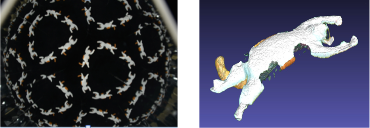
Figure 1: Kaleidoscopic imaging system. Left: kaleidoscopic projection of a 3D cat object. Right: a 3D reconstruction result.

2 Related work

In the context of kaleidoscopic imaging, Ihrke et al. [10] and Reshetouski and Ihrke[20, 19] have proposed a theory on modeling the chamber detection, segmentation, bounce tracing, shape-from-silhouette, etc. In these studies, however, the geometric calibration of the mirrors is simply achieved by detecting chessboards first[29], and then by estimating the mirror normals and the distances from chessboard 3D positions in the camera frame.

By considering kaleidoscopic imaging as a system of observing reflections of a single object via different mirrors, another possible approach is to utilize calibration techniques from such mirrored observations[24, 12, 22, 8, 27, 16]. While their original motivation is to estimate the 3D structure from its indirect views via mirrors, they can be used for calibrating the kaleidoscopic system by supposing the direct view were not available. For example, the orthogonality constraint on mirrored 3D points proposed by [27] can be considered as another approach for kaleidoscopic system calibration in [10, 20].

These conventional calibration approaches utilize 3D positions of a reference object and its reflections. That is, they first recover the 3D pose of the reference object from each of the virtual views, and then compute the mirror parameters from their 3D positions. While the first step and the second step can be done linearly, 3D pose estimation without nonlinear optimizations (i.e. reprojection error minimization) is not robust to observation noise.

On the other hand, the proposed method directly estimates the mirror parameters linearly from kaleidoscopic projections of a single 3D point of unknown geometry, i.e. without knowing its 3D position. Since our algorithm is based on a reprojection constraint, the result is as accurate as those with nonlinear optimizations.

3 Kaleidoscopic imaging system

Figure 2: Measurement model. A 3D point $\bm{p}$ is reflected to $\bm{p}^{\prime}$ by a mirror $\pi$ of normal $\bm{n}$ and distance $d$, and they are projected to $\bm{q}$ and $\bm{q}^{\prime}$ respectively.

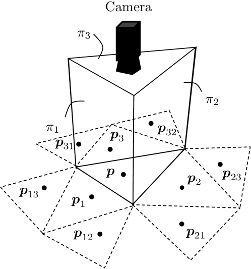
Figure 3: Kaleidoscopic imaging system. A 3D point $\bm{p}$ is reflected to $\bm{p}_{1}$, $\bm{p}_{2}$ and $\bm{p}_{3}$ by the mirrors $\pi_{1}$, $\pi_{2}$ and $\pi_{3}$ respectively.

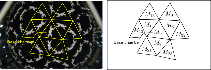
Figure 4: Chamber arrangement

Figure 2 illustrates the measurement model with a mirror. Let $\bm{p}$ denote a 3D point in the camera coordinate system. The mirror $\pi$ of normal $\bm{n}$ at distance $d$ from the camera generates its mirror as $\bm{p}^{\prime}$, and $\bm{p}$ and $\bm{p}^{\prime}$ are captured as $\bm{q}$ and $\bm{q}^{\prime}$ in the camera image

$$\lambda\bm{q}=A\bm{p},\quad\lambda^{\prime}\bm{q}^{\prime}=A\bm{p}^{\prime},$$ (1)

where $A$ is the intrinsic matrix of the camera calibrated beforehand, and $\lambda$ and $\lambda^{\prime}$ are the depths from the camera.

The 3D points $\bm{p}$ and $\bm{p}^{\prime}$ satisfy

$$\bm{p}=\bm{p}^{\prime}+2t\bm{n},$$ (2)

where $t$ denotes the distance from $\bm{p}$ to the mirror plane. Also the projection of $\bm{p}^{\prime}$ to $\bm{n}$ gives

$$t+d=-\bm{n}^{\top}\bm{p}^{\prime}.$$ (3)

These two equations yield

$$\bm{p}=-2(\bm{n}^{\top}\bm{p}^{\prime}+d)\bm{n}+\bm{p}^{\prime},$$ (4)

and can be rewritten as

$$\tilde{\bm{p}}=S\tilde{\bm{p}}^{\prime}=\begin{bmatrix}H&-2d\bm{n}\\ \bm{0}_{1\times 3}&1\end{bmatrix}\tilde{\bm{p}}^{\prime},$$ (5)

where $H=I_{3{\times}3}-2\bm{n}\bm{n}^{\top}$ is a $3{\times}3$ Householder matrix, $\tilde{x}$ denotes the homogeneous coordinate of $x$, and $\bm{0}_{m{\times}n}$ denotes the $m{\times}n$ zero matrix.

Kaleidoscopic imaging system utilize multiple mirrors to generate multiple viewpoints virtually (Figure 3), and the images captured by the camera consist of chambers corresponding to images captured by the real and the virtual cameras as shown in Figure 4. Here we assume three mirrors system while our calibration can be adopted to other configurations.

Let $M_{0}$ denote the base chamber corresponding to the direct view of the target. The three mirrors $\pi_{1}$, $\pi_{2}$ and $\pi_{3}$ generate first reflection chambers $M_{1}$, $M_{2}$ and $M_{3}$ respectively. These three mirrors also generate virtual mirrors $\pi_{ij}$ by mirroring $\pi_{j}$ by $\pi_{i}\>(i,j=1,2,3,\>i\neq j)$. The matrices $S_{ij}$ and $H_{ij}$ of $\pi_{ij}$ are given by

$$\begin{split}S_{ij}&=S_{i}S_{j},\\ H_{ij}&=H_{i}H_{j},\end{split}$$ (6)

and the camera observes the second reflection chamber $M_{ij}$ as the mirror of $M_{j}$ by $\pi_{i}$. The third and further reflections are defined by

$$\Pi_{k=1}^{m}S_{i_{k}}\>(i_{k}=1,2,3,\>i_{k}\neq i_{k+1}),$$ (7)

where $m$ is the number of reflections.

The goal of our extrinsic calibration is to estimate the parameters $\bm{n}_{i}$ and $d_{i}$ of the real mirror $\pi_{i}$ from projections of a single 3D point in the base chamber $M_{0}$ and its mirrors in $M_{i}$, $M_{ij}$, and so on.

4 Single mirror calibration from projections of two 3D points

Suppose the camera observes a 3D point of unknown geometry $\bm{p}$. The mirror $\pi$ of matrix $S$ defined by the normal $\bm{n}$ and the distance $d$ reflects $\bm{p}$ to $\bm{p}^{\prime}=S\bm{p}$ (Eq (5)).

Based on the epipolar geometry[7, 28], $\bm{n}$, $\bm{p}$ and $\bm{p}^{\prime}$ are coplanar and satisfy

$$\left(\bm{n}\times\bm{p}\right)^{\top}\bm{p}^{\prime}=0.$$ (8)

By substituting $\bm{p}$ and $\bm{p}^{\prime}$ by $\lambda A^{-1}\bm{q}$ and $\lambda^{\prime}A^{-1}\bm{q}^{\prime}$ respectively (Eq (1)), we obtain

$$\bm{q}^{\top}A^{-\top}[\bm{n}]_{\times}^{\top}A^{-1}\bm{q}^{\prime}=0,$$ (9)

where $[\bm{n}]_{\times}$ denotes the $3\times 3$ skew-symmetric matrix representing the cross product by $\bm{n}$ and this is the essential matrix of this mirror-based binocular geometry[28].

By representing the normalized image coordinates of $\bm{q}$ and $\bm{q}^{\prime}$ by $(x,y,1)^{\top}=A^{-1}\bm{q}$ and $(x^{\prime},y^{\prime},1)^{\top}=A^{-1}\bm{q}^{\prime}$ respectively, Eq (9) can be rewritten as

$$\begin{pmatrix}y-y^{\prime}&x^{\prime}-x&xy^{\prime}-x^{\prime}y\end{pmatrix}\bm{n}=0.$$ (10)

This equation allows estimating $\bm{n}$ up to scale by using projections of more than or equal to two 3D points and their mirrors. Since $\bm{n}$ is a unit vector, we can obtain a unique solution by assuming the mirror is front-facing to the camera.

It should be noted the distance $d$ from the camera to the mirror cannot be estimated since it is identical to the scale factor.

5 Multiple mirrors calibration from kaleidoscopic projections of single 3D point

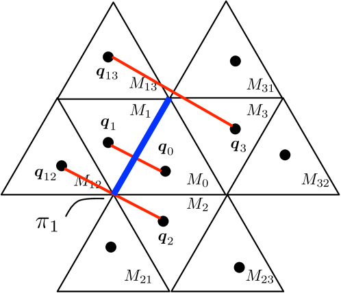
Figure 5: Corresponding points. Three pairs $\langle\bm{q}_{0},\bm{q}_{1}\rangle$, $\langle\bm{q}_{2},\bm{q}_{12}\rangle$ and $\langle\bm{q}_{3},\bm{q}_{13}\rangle$ (red) are available or mirror $\pi_{1}$ (blue)

This section introduces our linear algorithm which estimates the mirror normals and the distances from the kaleidoscopic projections of a single 3D point. Notice that the algorithm is first introduced by utilizing up to the second reflections, but they can be extended to third or further reflections intuitively as described later.

5.1 Mirror normals $\bm{n}_{1}$, $\bm{n}_{2}$, and $\bm{n}_{3}$

The algorithm in Section 4 realizes a mirror calibration on a per-mirror basis. That is, it can estimate the parameters of $\pi_{1}$, $\pi_{2}$ and $\pi_{3}$ independently. Furthermore, it can also estimate those of virtual mirrors such as $\pi_{13}$, $\pi_{23}$, and so forth.

However, such real mirror and virtual mirror parameters are not guaranteed to be consistent with each other and Eq (6) does not hold strictly. This results in inconsistent triangulations in 3D geometry estimation for example.

Instead of such mirror-wise estimations, this section proposes a new linear algorithm which calibrates the kaleidoscopic mirror parameters simultaneously by observing a single 3D point in the scene.

Suppose a 3D point $\bm{p}_{0}$ is projected to $\bm{q}_{0}$ in the base chamber, and its mirror $\bm{p}_{i}$ by $\pi_{i}$ is projected to $\bm{q}_{i}$ in the chamber $M_{i}$. Likewise, the second mirror $\bm{p}_{ij}$ by $\pi_{ij}$ is projected to $\bm{q}_{ij}$ in the chamber $M_{ij}$, and so forth.

Here $\bm{p}_{1}=S_{1}\bm{p}_{0}$ indicates that $\bm{q}_{0}$ and $\bm{q}_{1}$ satisfy Eq (10) and provide a constraint for estimating the mirror normal $\bm{n}_{1}$ of $\pi_{1}$ as described in Section 4. In addition, if $\bm{p}_{2}=S_{2}\bm{p}_{0}$ holds as well, we obtain $S_{1}\bm{p}_{2}=S_{1}S_{2}\bm{p}_{0}\Leftrightarrow\bm{p}_{12}=S_{1}\bm{p}_{2}$. That is, the projection $\bm{q}_{2}$ corresponding to the first reflection $\bm{p}_{2}$ and the projection $\bm{q}_{12}$ corresponding to the second reflection $\bm{p}_{12}$ also satisfy Eq (10) on $\bm{n}_{1}$. Similarly, if $\bm{p}_{3}=S_{3}\bm{p}_{0}$ holds, $\bm{q}_{3}$ and $\bm{p}_{12}$ provides a linear constraint on $\bm{n}_{1}$ as well. From these three constraints, $\bm{n}_{1}$ can be estimated by solving

$$\begin{bmatrix}y_{0}-y_{1}&x_{1}-x_{0}&x_{0}y_{1}-x_{1}y_{0}\\ y_{2}-y_{12}&x_{12}-x_{2}&x_{2}y_{12}-x_{12}y_{2}\\ y_{3}-y_{13}&x_{13}-x_{3}&x_{3}y_{13}-x_{13}y_{3}\\ \end{bmatrix}\bm{n}_{1}=\bm{0}_{3{\times}1}.$$ (11)

Similarly, $\bm{n}_{2}$ and $\bm{n}_{3}$ can be estimated by solving

$$\begin{bmatrix}y_{0}-y_{2}&x_{2}-x_{0}&x_{0}y_{2}-x_{2}y_{0}\\ y_{3}-y_{23}&x_{23}-x_{3}&x_{3}y_{23}-x_{23}y_{3}\\ y_{2}-y_{21}&x_{21}-x_{1}&x_{1}y_{21}-x_{21}y_{1}\\ \end{bmatrix}\bm{n}_{2}=\bm{0}_{3{\times}1},$$ (12)

and

$$\begin{bmatrix}y_{0}-y_{3}&x_{3}-x_{0}&x_{0}y_{3}-x_{3}y_{0}\\ y_{1}-y_{31}&x_{31}-x_{1}&x_{1}y_{31}-x_{31}y_{1}\\ y_{2}-y_{32}&x_{32}-x_{2}&x_{2}y_{32}-x_{32}y_{2}\end{bmatrix}\bm{n}_{3}=\bm{0}_{3{\times}1}.$$ (13)

An important observation in this simple algorithm is the fact that (1) this is a linear algorithm while it utilizes multiple reflections, and (2) the estimated normals $\bm{n}_{1}$, $\bm{n}_{2}$ and $\bm{n}_{3}$ are enforced to be consistent with each other while they are computed on a per-mirror basis apparently.

The first point is realized by using not the multiple reflections of a 3D position but their 2D projections. Intuitively a reasonable formalization of kaleidoscopic projection is to define a real 3D point in the scene, and then to express each of the projections of its reflections by Eq (5) coincides with the observed 2D position as introduced in Section 5.3 later. This expression, however, is nonlinear in the normals $\bm{n}_{i}\>(i=1,2,3)$ (e.g. $\bm{p}_{12}=S_{1}S_{2}\bm{p}_{0}$). On the other hand, projections of such multiple reflections can be associated as a result of single reflection by Eq (10) directly (e.g. $\bm{n}_{1}$ with $\bm{q}_{12}$ and $\bm{q}_{2}$ as the projections of $\bm{p}_{12}$ and $S_{2}\bm{p}_{0}$ respectively). As a result, we can utilize 2D projections of multiple reflections in the linear systems above.

This explains the second point as well. The above constraint on $\bm{q}_{12}$, $\bm{q}_{2}$ and $\bm{n}_{1}$ in Eq (11) assumes $\bm{p}_{2}=S_{2}\bm{p}_{0}$ being satisfied, and it is enforced by $(A^{-1}\bm{q}_{2}\times A^{-1}\bm{q}_{0})^{\top}\bm{n}_{2}=0$ in the first row of Eq (12). Inversely, on estimating $\bm{n}_{1}$ by Eq (11), it enforces $\bm{p}_{1}=S_{1}\bm{p}_{0}$ for Eqs (12) and (13).

It should be noted that this algorithm can be extended to third or further reflections intuitively. For example, if $\bm{p}_{23}$ and its reflection by $\pi_{1}$ is observable as $\lambda_{123}\bm{q}_{123}=A\bm{p}_{123}=AS_{1}\bm{p}_{23}$, then it provides

$$\left(y_{23}-y_{123},x_{23}-x_{123},x_{23}y_{123}-x_{123}y_{23}\right)\bm{n}_{1}=0,$$ (14)

and can be integrated with Eq (11).

5.2 Mirror distances $d_{1}$, $d_{2}$, and $d_{3}$

Once the mirror normals $\bm{n}_{1}$, $\bm{n}_{2}$, and $\bm{n}_{3}$ are given linearly, the mirror distances $d_{1}$, $d_{2}$, and $d_{3}$ can also be estimated linearly as follows.

Kaleidoscopic reprojection constraint

The perspective projection Eq (1) indicates that a 3D point $\bm{p}_{i}$ and its projection $\bm{q}_{i}$ should satisfy the collinearity constraint:

$$(A^{-1}\bm{q}_{i})\times\bm{p}_{i}=\bm{x}_{i}\times\bm{p}_{i}=\bm{0}_{3{\times}1},$$ (15)

where $\bm{x}_{i}=\begin{pmatrix}x_{i}&y_{i}&1\end{pmatrix}^{\top}$ is the normalized camera coordinate of $\bm{q}_{i}$ as defined earlier. Since the mirrored points $\bm{p}_{i}\>(i=1,2,3)$ are then given by Eq (5) as

$$\begin{split}\bm{p}_{i}&=H_{i}\bm{p}_{0}-2d_{i}\bm{n}_{i},\end{split}$$ (16)

and we obtain

$$\begin{split}\bm{x}_{i}\times\bm{p}_{i}&=\bm{x}_{i}\times(H_{i}\bm{p}_{0}-2d_{i}\bm{n}_{i})\\ &=[\bm{x}_{i}]_{\times}\begin{bmatrix}H_{i}&-2\bm{n}_{i}\end{bmatrix}\begin{bmatrix}\bm{p}_{0}\\ d_{i}\end{bmatrix}\\ &=\bm{0}_{3{\times}1}.\end{split}$$ (17)

Similarly, the second reflection $\bm{p}_{ij}$ is also collinear with its projection $\bm{q}_{ij}$:

$$\begin{split}&(A^{-1}\bm{q}_{ij})\times\bm{p}_{ij}\\ =&[\bm{x}_{ij}]_{\times}(H_{i}\bm{p}_{j}-2d_{i}\bm{n}_{i})\\ =&[\bm{x}_{ij}]_{\times}\left(H_{i}\left(H_{j}\bm{p}_{0}-2d_{j}\bm{n}_{j}\right)-2d_{i}\bm{n}_{i}\right)\\ =&[\bm{x}_{ij}]_{\times}\begin{bmatrix}H_{i}H_{j}&-2\bm{n}_{i}&-2H_{i}\bm{n}_{j}\end{bmatrix}\begin{bmatrix}\bm{p}_{0}\\ d_{i}\\ d_{j}\end{bmatrix}\\ =&\bm{0}_{3{\times}1}.\end{split}$$ (18)

By using these constraints, we obtain a linear system of $\bm{p}_{0}$, $d_{1}$, $d_{2}$, and $d_{3}$:

$$\begin{split}&\begin{bmatrix}[\bm{x}_{0}]_{\times}&\bm{0}_{3{\times}1}&\bm{0}_{3{\times}1}&\bm{0}_{3{\times}1}\\ h_{1}&-2[\bm{x}_{1}]_{\times}\bm{n}_{1}&\bm{0}_{3{\times}1}&\bm{0}_{3{\times}1}\\ h_{2}&\bm{0}_{3{\times}1}&-2[\bm{x}_{2}]_{\times}\bm{n}_{2}&\bm{0}_{3{\times}1}\\ h_{3}&\bm{0}_{3{\times}1}&\bm{0}_{3{\times}1}&-2[\bm{x}_{3}]_{\times}\bm{n}_{3}\\ h^{\prime}_{1,2}&-2[\bm{x}_{12}]_{\times}\bm{n}_{1}&-2h^{\prime\prime}_{1,2}&\bm{0}_{3{\times}1}\\ h^{\prime}_{2,1}&-2h^{\prime\prime}_{2,1}&-2[\bm{x}_{21}]_{\times}\bm{n}_{2}&\bm{0}_{3{\times}1}\\ h^{\prime}_{2,3}&\bm{0}_{3{\times}1}&-2[\bm{x}_{23}]_{\times}\bm{n}_{2}&-2h^{\prime\prime}_{2,3}\\ h^{\prime}_{3,2}&\bm{0}_{3{\times}1}&-2h^{\prime\prime}_{3,2}&-2[\bm{x}_{32}]_{\times}\bm{n}_{3}\\ h^{\prime}_{3,1}&-2h^{\prime\prime}_{3,1}&\bm{0}_{3{\times}1}&-2[\bm{x}_{31}]_{\times}\bm{n}_{3}\\ h^{\prime}_{1,3}&-2[\bm{x}_{13}]_{\times}\bm{n}_{1}&\bm{0}_{3{\times}1}&-2h^{\prime\prime}_{1,3}\\ \end{bmatrix}\begin{bmatrix}\bm{p}_{0}\\ d_{1}\\ d_{2}\\ d_{3}\end{bmatrix}\\ =&K\begin{bmatrix}\bm{p}_{0}\\ d_{1}\\ d_{2}\\ d_{3}\end{bmatrix}=\bm{0}_{30{\times}1},\end{split}$$ (19)

where $h_{i}=[\bm{x}_{i}]_{\times}H_{i}$, $h^{\prime}_{i,j}=[\bm{x}_{ij}]_{\times}H_{i}H_{j}$, $h^{\prime\prime}_{i,j}=[\bm{x}_{ij}]_{\times}H_{i}\bm{n}_{j}$. By computing the eigenvector corresponding to the smallest eigenvalue of $K^{\top}K$, $(\bm{p}_{0},d_{1},d_{2},d_{3})^{\top}$ can be determined up to a scale factor. In this paper, we choose the scale that normalizes $d_{1}=1$.

Notice that Eq (19) apparently has 30 equations, but only 20 of them are linearly independent. This is simply because each of the cross products by Eqs (15) and (18) has only two independent constraints by definition.

Also, as discussed in Section 5.1, the above algorithm can be extended to third or further reflections as well. For example, given the reflection of $\bm{p}_{23}$ by $\pi_{1}$ as $\lambda_{123}\bm{q}_{123}=A\bm{p}_{123}=AS_{1}\bm{p}_{23}$, then it provides

$$[\bm{x}_{123}]_{\times}\begin{bmatrix}(H_{1}H_{2}H_{3})^{\top}\\ -2\bm{n}_{1}^{\top}\\ -2(H_{1}\bm{n}_{2})^{\top}\\ -2(H_{1}H_{2}\bm{n}_{3})^{\top}\end{bmatrix}^{\top}\begin{bmatrix}\bm{p}_{0}\\ d_{1}\\ d_{2}\\ d_{3}\end{bmatrix}=\bm{0}_{3{\times}1},$$ (20)

and can be integrated with Eq (19).

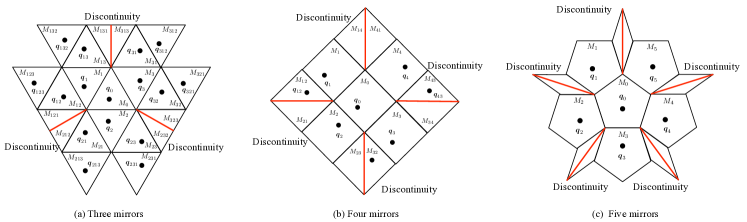
Figure 6: Kaleidoscopic imaging system using (a) three, (b) four, and (c) five mirrors. Discontinuities (red lines) appear on the boundaries of overlapping chambers.

Notice that our method works as long as the second reflections by non-parallel mirrors are given regardless of the number of the mirrors. However, in cases of more than three mirrors, discontinuities are more likely to happen in general, and finding the second reflections itself become difficult (Figure 6).

5.3 Kaleidoscopic bundle adjustment

Once estimated the mirror normals $\bm{n}_{i}$ and the distances $d_{i}\>(i=1,2,3)$ linearly, the triangulation from kaleidoscopic projections of a single 3D point can be given in a DLT manner by solving:

$$K^{\prime}\bm{p}_{0}=-K^{\prime\prime}\bm{d},$$ (21)

as $\bm{p}_{0}^{\ast}=-(K^{\prime\top}K^{\prime})^{-1}K^{\prime\top}K^{\prime\prime}\bm{d}$, where $\bm{d}=(d_{1},d_{2},d_{3})^{\top}$, $K^{\prime}$ is the $30{\times}3$ matrix corresponding to the first three columns of $K$:

$$\begin{split}&K^{\prime}=\\ &\begin{bmatrix}[\bm{x}_{0}]_{\times}^{\top},h_{1}^{\top},h_{2}^{\top},h_{3}^{\top},h^{{}^{\prime}\top}_{1,2},h^{{}^{\prime}\top}_{2,1},h^{{}^{\prime}\top}_{2,3},h^{{}^{\prime}\top}_{3,2},h^{{}^{\prime}\top}_{3,1},h^{{}^{\prime}\top}_{1,3}\end{bmatrix}^{\top},\end{split}$$ (22)

and $K^{\prime\prime}$ is the $30{\times}3$ matrix corresponding to the 4th to 7th columns of $K$:

$$K^{\prime\prime}=\begin{bmatrix}\bm{0}_{3{\times}1}&\bm{0}_{3{\times}1}&\bm{0}_{3{\times}1}\\ -2[\bm{x}_{1}]_{\times}\bm{n}_{1}&\bm{0}_{3{\times}1}&\bm{0}_{3{\times}1}\\ \bm{0}_{3{\times}1}&-2[\bm{x}_{2}]_{\times}\bm{n}_{2}&\bm{0}_{3{\times}1}\\ \bm{0}_{3{\times}1}&\bm{0}_{3{\times}1}&-2[\bm{x}_{3}]_{\times}\bm{n}_{3}\\ -2[\bm{x}_{12}]_{\times}\bm{n}_{1}&-2h^{\prime\prime}_{1,2}&\bm{0}_{3{\times}1}\\ -2h^{\prime\prime}_{2,1}&-2[\bm{x}_{21}]_{\times}\bm{n}_{2}&\bm{0}_{3{\times}1}\\ \bm{0}_{3{\times}1}&-2[\bm{x}_{23}]_{\times}\bm{n}_{2}&-2h^{\prime\prime}_{2,3}\\ \bm{0}_{3{\times}1}&-2h^{\prime\prime}_{3,2}&-2[\bm{x}_{32}]_{\times}\bm{n}_{3}\\ -2h^{\prime\prime}_{3,1}&\bm{0}_{3{\times}1}&-2[\bm{x}_{31}]_{\times}\bm{n}_{3}\\ -2[\bm{x}_{13}]_{\times}\bm{n}_{1}&\bm{0}_{3{\times}1}&-2h^{\prime\prime}_{1,3}\\ \end{bmatrix}.$$ (23)

By reprojecting this $\bm{p}_{0}^{\ast}$ to each of the chambers as

$$\begin{split}\lambda\hat{\bm{q}}_{0}&=A\bm{p}_{0}^{\ast},\\ \lambda\hat{\bm{q}}_{i}&=AS_{i}\bm{p}_{0}^{\ast}\>(i=1,2,3),\\ \lambda\hat{\bm{q}}_{i,j}&=AS_{i}S_{j}\bm{p}_{0}^{\ast}\>(i,j=1,2,3,\>i\neq j),\end{split}$$ (24)

we obtain a reprojection error as

$$\begin{split}&\bm{E}(\bm{n}_{1},\bm{n}_{2},\bm{n}_{3},d_{1},d_{2},d_{3})\\ &=\begin{bmatrix}\bm{q}_{0}-\hat{\bm{q}}_{0},\bm{e}_{1},\bm{e}_{2},\bm{e}_{3},\bm{e}^{\prime}_{1,2},\bm{e}^{\prime}_{2,1},\bm{e}^{\prime}_{2,3},\bm{e}^{\prime}_{3,2},\bm{e}^{\prime}_{3,1},\bm{e}^{\prime}_{1,3}\end{bmatrix}^{\top},\end{split}$$ (25)

where $\bm{e}_{i}=\bm{q}_{i}-\hat{\bm{q}}_{i}$ and $\bm{e}^{\prime}_{i,j}=\bm{q}^{\prime}_{i,j}-\hat{\bm{q}}^{\prime}_{i,j}$. By minimizing $||\bm{E}(\cdot)||^{2}$ nonlinearly over $\bm{n}_{1},\bm{n}_{2},\bm{n}_{3},d_{1},d_{2},d_{3}$, we obtain a best estimate of the mirror normals and the distances.

6 Evaluations

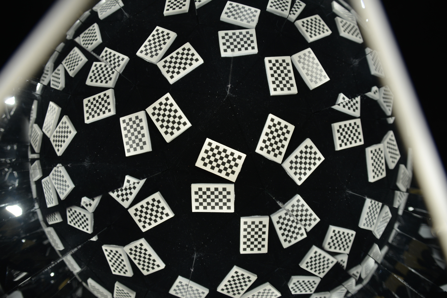
Figure 7: A capture of a chessboard used as the reference object for conventional methods

To demonstrate the performance of the proposed algorithm, this section provides evaluations using synthesized and real images in comparison with the following two conventional algorithms both utilize a reference object of known geometry as shown in Figure 7.

Baseline

Since the 3D geometry of the reference object is known, the 3D positions of the real image $\bm{p}_{0}^{(l)}$ and their reflections $\bm{p}_{i}^{(l)}$ and $\bm{p}_{i,j}^{(l)}$ can be estimated by solving PnP[14]. Here the superscript ^(l) indicates the $l$th landmark in the reference object. Once $L$ such landmark 3D positions are given, then the mirror normals can be computed simply by

$$\begin{split}\bm{n}_{1}=\sum_{l}^{L}\bm{l}_{1,2,3}^{(l)}/\left\|\sum_{l}^{L}\bm{l}_{1,2,3}^{(l)}\right\|,\\ \bm{n}_{2}=\sum_{l}^{L}\bm{l}_{2,3,1}^{(l)}/\left\|\sum_{l}^{L}\bm{l}_{2,3,1}^{(l)}\right\|,\\ \bm{n}_{3}=\sum_{l}^{L}\bm{l}_{3,1,2}^{(l)}/\left\|\sum_{l}^{L}\bm{l}_{3,1,2}^{(l)}\right\|,\\ \end{split}$$ (26)

where $\bm{l}_{i,j,k}^{(l)}=\bm{p}_{i}^{(l)}-\bm{p}_{0}^{(l)}+\bm{p}_{ij}^{(l)}-\bm{p}_{j}^{(l)}+\bm{p}_{ik}^{(l)}-\bm{p}_{k}^{(l)}$, and then the mirror distances can be computed by

$$\begin{split}d_{1}=\frac{1}{6L}\bm{n}_{1}^{\top}\sum_{l}^{L}\left(\sum_{i=0}^{3}\left(\bm{p}_{i}^{(l)}\right)+\bm{p}_{12}^{(l)}+\bm{p}_{13}^{(l)}\right),\\ d_{2}=\frac{1}{6L}\bm{n}_{2}^{\top}\sum_{l}^{L}\left(\sum_{i=0}^{3}\left(\bm{p}_{i}^{(l)}\right)+\bm{p}_{23}^{(l)}+\bm{p}_{21}^{(l)}\right),\\ d_{3}=\frac{1}{6L}\bm{n}_{3}^{\top}\sum_{l}^{L}\left(\sum_{i=0}^{3}\left(\bm{p}_{i}^{(l)}\right)+\bm{p}_{31}^{(l)}+\bm{p}_{32}^{(l)}\right).\\ \end{split}$$ (27)

Notice that the above PnP procedure requires a non-linear reprojection error minimization process in practice.

Takahashi et al. [27]

As pointed out by Takahashi et al. [27], two 3D points $\bm{p}_{i}$ and $\bm{p}_{j}$ defined as reflections of a 3D point by different mirrors of normal $\bm{n}_{i}$ and $\bm{n}_{j}$ respectively satisfy an orthogonality constraint:

$$\left(\bm{p}_{i}-\bm{p}_{j}\right)^{\top}\left(\bm{n}_{i}\times\bm{n}_{j}\right)=\left(\bm{p}_{i}-\bm{p}_{j}\right)^{\top}\bm{m}_{ij}=0.$$ (28)

As illustrated by Figure 8, this constraint on $\bm{m}_{12}$ holds for four pairs $\langle\bm{p}_{1},\bm{p}_{2}\rangle$, $\langle\bm{p}_{0},\bm{p}_{21}\rangle$, $\langle\bm{p}_{12},\bm{p}_{0}\rangle$, and $\langle\bm{p}_{13},\bm{p}_{23}\rangle$ as the reflections of $\bm{p}_{0}$, $\bm{p}_{1}$, $\bm{p}_{2}$, and $\bm{p}_{3}$ respectively. Similarly, $\langle\bm{p}_{2},\bm{p}_{3}\rangle$, $\langle\bm{p}_{21},\bm{p}_{31}\rangle$, $\langle\bm{p}_{0},\bm{p}_{32}\rangle$, and $\langle\bm{p}_{23},\bm{p}_{0}\rangle$ can be used for computing $\bm{m}_{23}=\bm{n}_{2}\times\bm{n}_{3}$, and $\langle\bm{p}_{3},\bm{p}_{1}\rangle$, $\langle\bm{p}_{31},\bm{p}_{0}\rangle$, $\langle\bm{p}_{32},\bm{p}_{12}\rangle$, and $\langle\bm{p}_{0},\bm{p}_{13}\rangle$ can be used for $\bm{m}_{31}=\bm{n}_{3}\times\bm{n}_{1}$. Once obtained the intersection vectors $\bm{m}_{12}$, $\bm{m}_{23}$ and $\bm{m}_{31}$, the mirror normals and the distances can be estimated linearly as described in [27].

The following three error metrics are used in this section in order to evaluate the performance of the proposed method in comparison with the above-mentioned conventional approaches quantitatively. The average estimation error of normal $E_{\bm{n}}$ measures the average angular difference from the ground truth by

$$E_{\bm{n}}=\frac{1}{3}\sum_{i=1}^{3}\left|\cos^{-1}(\bm{n}_{i}^{\top}\check{\bm{n}}_{i})\right|,$$ (29)

where $\check{\bm{n}}_{i}\>(i=1,2,3)$ denotes the ground truth of the normal $\bm{n}_{i}$. The average estimation error of distance $E_{d}$ is defined as the average $L_{1}$-norm to the ground truth:

$$E_{d}=\frac{1}{3}\sum_{i=1}^{3}|d_{i}-\check{d}_{i}|,$$ (30)

where $\check{d}_{i}\>(i=1,2,3)$ denotes the ground truth of the distance $d_{i}$. Also, the average reprojection error $E_{\mathrm{rep}}$ is defined as:

$$E_{\mathrm{rep}}=\frac{1}{10L}\sum_{l=1}^{L}\left|\bm{E}^{(l)}(\bm{n}_{1},\bm{n}_{2},\bm{n}_{3},d_{1},d_{2},d_{3})\right|,$$ (31)

where $\bm{E}^{(l)}(\cdot)$ denotes the reprojection error $\bm{E}(\cdot)$ defined by Eq (25) at $l$th point.

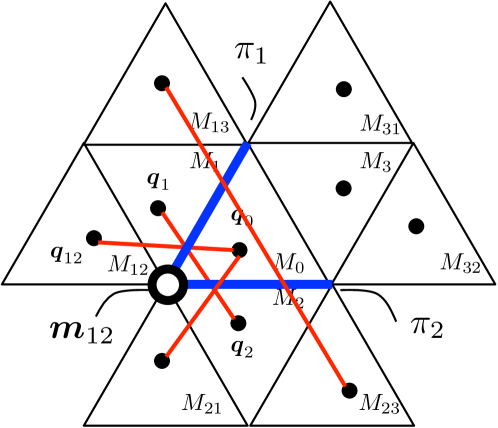
Figure 8: Corresponding points for the orthogonality constraint[27]. Four pairs $\langle\bm{p}_{1},\bm{p}_{2}\rangle$, $\langle\bm{p}_{0},\bm{p}_{21}\rangle$, $\langle\bm{p}_{12},\bm{p}_{0}\rangle$, and $\langle\bm{p}_{13},\bm{p}_{23}\rangle$ are available for the intersection $\bm{m}_{12}=\bm{n}_{1}\times\bm{n}_{2}$.

6.1 Quantitative evaluations with synthesized images

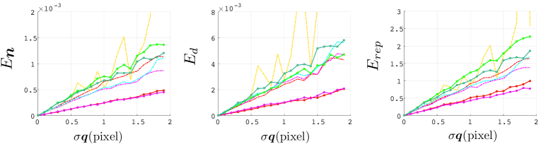
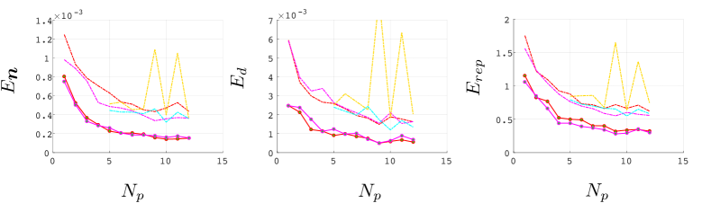
Figure 9: Estimation errors at different noise levels $\sigma_{\bm{q}}$. Legends are provided in Table 12.

Figure 10: Estimation errors at different numbers of reference points $N_{p}$. Legends are provided in Table 12.

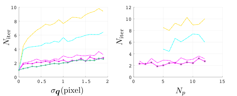
Figure 11: Number of iterations at different $\sigma_{\bm{q}}$ with $N_{p}=5$ (left) and at different $N_{p}$ with $\sigma_{\bm{q}}=1$ (right). Legends are provided in Table 12.

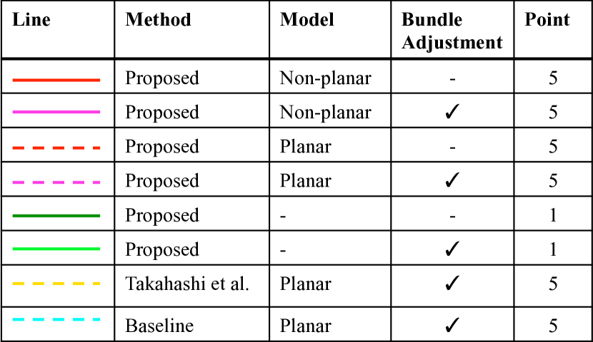
Figure 12: Configurations

This section provides a quantitative performance evaluation using synthesized dataset. A virtual camera and three mirrors are arranged according to the real setup (Figure 13). By virtually capturing 3D points simulating a reference object, the corresponding 2D kaleidoscopic projections used as the ground truth are generated first, and then random pixel noise is injected to them at each trial of calibration.

Figures 12, 12 and 12 report average estimation errors $E_{\bm{n}}$, $E_{d}$, $E_{\mathrm{rep}}$ over 100 trials at different noise levels and different numbers of reference points. In these figures $\sigma_{\bm{q}}$ denotes the standard deviation of zero-mean Gaussian pixel noise, $N_{p}$ denotes the number of 3D points used in the calibration, and $N_{\mathrm{iter}}$ denotes the number of iterations required by the kaleidoscopic bundle adjustment.

As shown in Table 12, the magenta and red lines denote the results by the proposed method with and without the non-linear optimization (Section 5.3). They use kaleidoscopic projections of non-planar random five 3D points, while the dashed red and magenta lines are the results with planar five points simulating the chessboard (Figure 7). The light and dark green lines are the results with a single 3D point generated randomly followed by the non-linear optimization or not.

The yellow and cyan dashed lines are the results by Takahashi et al. [27] and the baseline with the same five points for the red and magenta dashed lines. Notice that the baseline and Takahashi et al. [27] without the final non-linear optimization could not achieve comparable results (typically $E_{\mathrm{rep}}\gg 10$ pixel). Also these methods using 3D reference positions without applying non-linear refinement after a linear PnP[14] could not estimate valid initial parameters for the final non-linear optimization. Therefore, they are omitted in these figures. On the other hand, the final non-linear optimization for our method does not improve the result drastically. This is because our algorithm originally utilizes the reprojection error constraint.

From these results, we can conclude that (1) the proposed method can achieve comparable estimation linearly even with a single 3D point (dark green), and (2) the proposed method (red and magenta) with the same number 3D points used in the conventional methods (yellow and cyan) performs better, even without the final non-linear optimization.

Also in particular in the cases of $\sigma_{\bm{q}}\geq 1$, we can observe Takahashi et al. (yellow) do not show robust behavior. This is because the method degenerates obviously if the intersection vectors $\bm{m}_{12}$, $\bm{m}_{23}$ and $\bm{m}_{31}$ are parallel since the normal is recovered by $\bm{n}_{i}=\bm{m}_{ij}\times\bm{m}_{ki}$. Therefore if the estimated 3D reference points by PnP return the intersection vectors close to such a singular configuration due to noise, then it will not perform robustly[27, 1].

6.2 Qualitative evaluations with real images

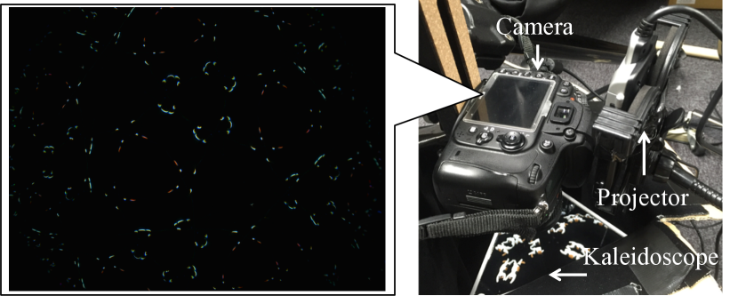
Figure 13: Capture setup

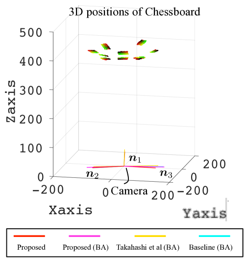
Figure 14: Calibration results. The colored lines in the bottom illustrate $d\bm{n}$ (i.e. the foot of perpendicular from the camera center) of each mirrors. The 10 patterns in the top illustrate the 3D points estimated by PnP.

Figure 13 shows our kaleidoscopic capture setup. The intrinsic parameter $A$ of the camera (Nikon D600, $6016{\times}4016$ resolution) is calibrated beforehand[29], and it observes the target object cat (about $4\times 5\times 1$ cm) with three planar first surface mirrors. The projector (MicroVision SHOWWX+ Laser Pico Projector, $848{\times}480$ resolution) is used to cast line patterns to the object for simplifying the correspondence search problem in a light-sectioning fashion (Figure 13 left), and the projector itself is not involved in the calibration w.r.t. the camera and the mirrors.

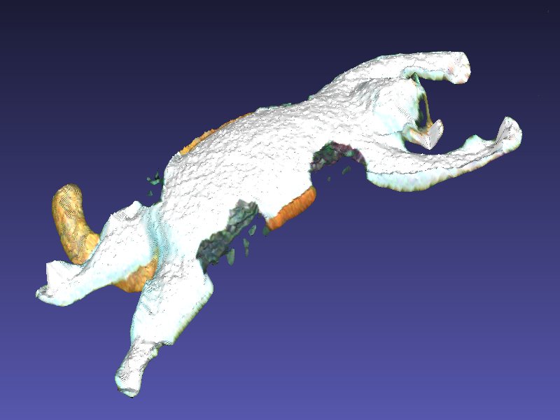
Figure 15: Reconstructed 3D shape

Figures 7 shows a captured image of a chessboard, and Figure 14 shows the mirror normals and distances calibrated by the proposed method and the conventional methods. While the estimated mirror parameters look close to each other, the reprojection errors $E_{\mathrm{rep}}$ of the proposed, the baseline, and Takahashi et al. were 3.37, 4.75, and 13.6 pixels respectively. These reprojection errors are higher than simulation results and this is because of the localization accuracy of corresponding points and nonplanarity of mirrors. Figure 15 shows a 3D rendering of the estimated 3D shape using the mirror parameters calibrated by the proposed method, while the residual reprojection error indicates the parameters can be further improved for example through the 3D shape reconstruction process itself[4].

From these results, we can conclude that the proposed method performs reasonably and provides a sufficiently accurate calibration for 3D shape reconstruction.

7 Conclusion

This paper proposed a new linear calibration of kaleidoscopic mirror system from 2D kaleidoscopic projections of a single 3D point in the scene. The key point to realize our linear method is to utilize not 3D positions of multiple reflections but their 2D projections.

One of the advantages of our approach is the fact that the proposed method does not require knowing the 3D geometry of the 2D points for calibration, while the conventional methods require 2D-to-3D correspondences. This indicates that our method can utilize 3D points on the target object surface of unknown geometry, and this point is verified by the evaluations in which the proposed method with non-planar calibration points outperforms the conventional methods even without bundle adjustment.

Inversely, our method assumes the 2D correspondences are given a priori. This is not a trivial problem[19], and integration with such automatic correspondence search and chamber segmentation should be further investigated to realize a complete calibration procedure for kaleidoscopic imaging system.

References

• [1] A. Agrawal. Extrinsic camera calibration without a direct view using spherical mirror. In Proc. of ICCV, 2013.
• [2] K. Forbes, F. Nicolls, G. D. Jager, and A. Voigt. Shape-from-silhouette with two mirrors and an uncalibrated camera. In Proc. of ECCV, 2006.
• [3] M. Fuchs, M. Kächele, and S. Rusinkiewicz. Design and fabrication of faceted mirror arrays for light field capture. In Workshop on Vision, Modeling and Visualization, 2012.
• [4] Y. Furukawa and J. Ponce. Accurate camera calibration from multi-view stereo and bundle adjustment. IJCV, 84(3):257–268, 2009.
• [5] J. Gluckman and S. K. Nayar. Catadioptric stereo using planar mirrors. IJCV, 44(1):65–79, 2001.
• [6] A. Goshtasby and W. A. Gruver. Design of a single-lens stereo camera system. Pattern Recognition, 26(6):923 – 937, 1993.
• [7] R. I. Hartley and A. Zisserman. Multiple View Geometry in Computer Vision. Cambridge University Press, 2000.
• [8] J. A. Hesch, A. I. Mourikis, and S. I. Roumeliotis. Algorithmic Foundation of Robotics VIII, volume 57 of Springer Tracts in Advanced Robotics, chapter Mirror-Based Extrinsic Camera Calibration, pages 285–299. 2009.
• [9] P.-H. Huang and S.-H. Lai. Contour-based structure from reflection. In Proc. of CVPR, volume 1, pages 379–386, 2006.
• [10] I. Ihrke, I. Reshetouski, A. Manakov, A. Tevs, M. Wand, and H.-P. Seidel. A kaleidoscopic approach to surround geometry and reflectance acquisition. In CVPR Workshop on Computational Cameras and Displays, pages 29–36, 2012.
• [11] C. Inoshita, S. Tagawa, M. A. Mannan, Y. Mukaigawa, and Y. Yagi. Full-dimensional sampling and analysis of bssrdf. IPSJ Transactions on Computer Vision and Applications, 5:119–123, 2013.
• [12] R. Kumar, A. Ilie, J.-M. Frahm, and M. Pollefeys. Simple calibration of non-overlapping cameras with a mirror. In Proc. of CVPR, pages 1–7, 2008.
• [13] D. Lanman, D. Crispell, and G. Taubin. Surround structured lightning: 3-d scanning with orthographic illumination. In CVIU, pages 1107–1117, November 2009.
• [14] V. Lepetit, F. Moreno-Noguer, and P. Fua. Epnp: An accurate o(n) solution to the pnp problem. IJCV, 81(2), 2008.
• [15] M. Levoy, B. Chen, V. Vaish, M. Horowitz, I. McDowall, and M. Bolas. Synthetic aperture confocal imaging. In Proc. of SIGGRAPH, pages 825–834, 2004.
• [16] G. Long, L. Kneip, X. Li, X. Zhang, and Q. Yu. Simplified mirror-based camera pose computation via rotation averaging. In Proc. of CVPR, pages 1247–1255, 2015.
• [17] S. A. Nene and S. K. Nayar. Stereo with mirrors. In Proc. of ICCV, pages 1087–1094, 1998.
• [18] S. Nobuhara, T. Kashino, T. Matsuyama, K. Takeuchi, , and K. Fujii. A single-shot multi-path interference resolution for mirror-based full 3d shape measurement with a correlation-based tof camera. In Proc. of 3DV, 2016.
• [19] I. Reshetouski, A. M. iand Ayush Bhandari, R. Raskar, H.-P. Seidel, and I. Ihrke. Discovering the structure of a planar mirror system from multiple observations of a single point. In Proc. of CVPR, pages 89–96, 2013.
• [20] I. Reshetouski and I. Ihrke. Mirrors in Computer Graphics, Computer Vision and Time-of-Flight Imaging, pages 77–104. Springer Berlin Heidelberg, 2013.
• [21] I. Reshetouski, A. Manakov, H.-P. Seidel, and I. Ihrke. Three-dimensional kaleidoscopic imaging. In Proc. of CVPR, pages 353–360, 2011.
• [22] R. Rodrigues, P. Barreto, and U. Nunes. Camera pose estimation using images of planar mirror reflections. In Proc. of ECCV, pages 382–395, 2010.
• [23] P. Sen, B. Chen, G. Garg, S. R. Marschner, M. Horowitz, M. Levoy, and H. P. A. Lensch. Dual photography. In Proc. of SIGGRAPH, pages 745–755, 2005.
• [24] P. Sturm and T. Bonfort. How to compute the pose of an object without a direct view. In Proc. of ACCV, pages 21–31, 2006.
• [25] S. Tagawa, Y. Mukaigawa, and Y. Yagi. 8-d reflectance field for computational photography. In Proc. of ICPR, pages 2181–2185, 2012.
• [26] T. Tahara, R. Kawahara, S. Nobuhara, and T. Matsuyama. Interference-free epipole-centered structured light pattern for mirror-based multi-view active stereo. In Proc. of 3DV, pages 153–161, 2015.
• [27] K. Takahashi, S. Nobuhara, and T. Matsuyama. A new mirror-based extrinsic camera calibration using an orthogonality constraint. In Proc. of CVPR, pages 1051–1058, 2012.
• [28] X. Ying, K. Peng, Y. Hou, S. Guan, J. Kong, and H. Zha. Self-calibration of catadioptric camera with two planar mirrors from silhouettes. TPAMI, 35(5):1206–1220, 2013.
• [29] Z. Zhang. A flexible new technique for camera calibration. TPAMI, 22:1330–1334, 1998.