Pythagorean theorem of Sharpe ratio

Abstract

In the present paper, using a replica analysis, we examine the portfolio optimization problem handled in previous work and discuss the minimization of investment risk under constraints of budget and expected return for the case that the distribution of the hyperparameters of the mean and variance of the return rate of each asset are not limited to a specific probability family. Findings derived using our proposed method are compared with those in previous work to verify the effectiveness of our proposed method. Further, we derive a Pythagorean theorem of the Sharpe ratio and macroscopic relations of opportunity loss. Using numerical experiments, the effectiveness of our proposed method is demonstrated for a specific situation.

PACS number(s)

89.65.Gh, 89.90.+n, 02.50.-r

I Introduction

Nowadays, most financial activities interact with each other on a global scale and our lives have been influenced, either directly or indirectly, by a number of financial crises. The lessons of the financial crisis include the need to take personal effort to preserve our assets. In this atmosphere and as reforms advance, the importance of making proper investments and managing risk has been recognized. Generally speaking, investment means paying a cost in anticipation of future return and often involves risk. Markowitz pointed out the importance of investment management and first laid out the portfolio optimization problem which is the framework for analyzing mathematically the optimal asset management strategy Markowitz1952 ; Markowitz1959 . Several studies following this pioneering work have been carried out Bodie ; Luenberger ; Prigent ; Ang ; Francis ; Elton . Recently, there has been much such research that takes the viewpoint of complex systems and actively applies analytical approaches refined in outside research fields, such as replica analysis, belief propagation, and random matrix theory, to the portfolio optimization problem Ciliberti1 ; Ciliberti2 ; Caccioli ; Pafka ; Shinzato-2015-PLOS7 ; Shinzato-2015-PLOS8 ; Shinzato-2016-PRE12 ; Shinzato-2011-IEICE ; Kondor-2016-with-no-short-selling ; Shinzato-2017-JSTAT2 ; Shinzato-ve-fixed2016 ; Shinzato-2016-PRE11 ; VH .

Table 1: Targets of previous studies. In the context of statistical physics, the models are related to the Hamiltonian and the constraints correspond to the priors.

Researchers	Model	Constraints	Optimizations	Analysis approaches
Ciliberti, Ciliberti et al. Ciliberti1 ; Ciliberti2	absolute deviation model, expected shortfall model	budget	minimization	replica analysis
Caccioli et al. Caccioli	expected shortfall mode, max loss model	budget	minimization	replica analysis
Pafka et al. Pafka	mean-variance model	budget	minimization	random matrix approach
Shinzato Shinzato-2015-PLOS7	mean-variance model	budget	minimization	replica analysis
Shinzato et al. Shinzato-2015-PLOS8	any model	budget	minimization	belief propagation
Shinzato Shinzato-2016-PRE12	mean-variance model	budget	minimization	replica analysis, belief propagation
Shinzato, Kondor et al. Shinzato-2011-IEICE ; Kondor-2016-with-no-short-selling	mean-variance model	budget, short selling	minimization	replica analysis
Shinzato Shinzato-2017-JSTAT2	mean-variance model	budget, investment concentration	minimization	replica analysis
Shinzato Shinzato-ve-fixed2016	mean-variance model	budget, investment risk	minimization and maximization	replica analysis
Shinzato Shinzato-2016-PRE11	mean-variance model	budget, expected return, investment risk	minimization and maximization	replica analysis
Varga-Haszonits et al. VH	a specific model	budget, expected return	minimization and maximization	replica analysis

Among such research (see Table 1), Ciliberti et al. described a diversified investment system using the Boltzmann distribution to analyze the optimal portfolio for minimizing risk under a budget constraint. In particular, they analyzed the minimal investment risk of the absolute deviation model and the expected shortfall model using the ground state in the absolute zero temperature limit (that is, the optimal state of this optimization problem) Ciliberti1 ; Ciliberti2 . Moreover, Caccioli et al. examined the expected shortfall model with $L_{2}$ regularization and max loss model as a special case of it by using replica analysis and identified the typical behavior of the optimal asset management strategy Caccioli . Furthermore, Pafka et al. discussed in detail the behavior of the investment risk which is defined using the variance-covariance matrix of the random weighted sums of each component of the lower triangular matrix which can be extracted from the true variance-covariance matrix with respect to the return rate of assets by using Cholesky decomposition and the in-sample risk by using the asymptotical spectrum of a random matrix which is generated by a given return rate Pafka . Subsequently, Shinzato analyzed one of the portfolio optimization problems, the mean–variance model, and showed that the minimal investment risk and its investment concentration satisfy the self-averaging property using the large deviation principle Shinzato-2015-PLOS7 . Shinzato also compared the minimal investment risk per asset derived using replica analysis with the minimal expected investment risk per asset derived using operations research from a unified viewpoint of stochastic optimization and pointed out that a portfolio which can minimize the expected investment risk does not necessarily minimize the investment risk. Furthermore, Shinzato et al. developed a faster algorithm for finding the optimal portfolio which can minimize the risk function by using the belief propagation method, which is often used in probabilistic inference, and verified that the computation time of the algorithm is on the order of the square of the number of assets (whereas the standard algorithm requires on the order of the cube of the number of assets computation time). Moreover, they also clarified that the Konno–Yamazaki conjecture which was previously confirmed in annealed disordered systems also holds true in quenched disordered systems Shinzato-2015-PLOS8 . Additionally, Shinzato used the portfolio optimization problem of Ref. Shinzato-2015-PLOS7 and examined the portfolio which can minimize the investment risk under a budget constraint for the case that the variances of the return rates of the assets are not unique using replica analysis and belief propagation Shinzato-2016-PRE12 . Shinzato also investigated the minimization of investment risk under constraints of budget and short selling by using replica analysis and showed that this investment system involves a phase transition. Further, he developed a faster algorithm based on belief propagation for obtaining the optimal portfolio Shinzato-2011-IEICE . In addition, Kondor et al. analyzed the same portfolio optimization problem for the case that the variance of the return rate of each asset is distinct using replica analysis and reconfirmed that this disordered system involves a phase transition Kondor-2016-with-no-short-selling . Furthermore, Shinzato also used the portfolio optimization problem handled in Ref. Shinzato-2015-PLOS7 to examine the minimization of investment risk under constraints of both budget and investment concentration by using replica analysis; in this context, he analyzed the optimization of investment concentration under constraints of budget and investment risk from a unified viewpoint of stochastic optimization and duality Shinzato-2017-JSTAT2 ; Shinzato-ve-fixed2016 . In addition, Shinzato used the portfolio optimization problem handled in previous work Shinzato-2015-PLOS7 to examine the minimization of investment risk under constraints of budget and expected return for the case that the variance of the return rate is the same for all assets by using replica analysis Shinzato-2016-PRE11 . Moreover, he also analyzed the maximization of expected returns under constraints of budget and investment risk and pointed out the importance of duality for assessing these optimization problems. Further, Varga-Haszonits et al. examined the minimization of a particular risk function (the sample variance with respect to the deviation between the return and its sample average) under constraints of budget and expected return by using replica analysis and carried out a stability analysis of the replica symmetric solution derived using replica analysis VH .

As discussed above, several previous studies which further refined the model introduced in Ref. Shinzato-2015-PLOS7 have been reported Shinzato-2016-PRE12 ; Shinzato-2016-PRE11 . The findings of these studies are closely linked, which makes it possible to use them to solve an important problem. Namely, in Ref. Shinzato-2016-PRE11 , the minimization of investment risk under constraints of budget and expected return for the case that the variance of the return rate of each asset is unique was discussed in detail, whereas in Ref. Shinzato-2016-PRE12 , the minimization of investment risk under a budget constraint for the case that the variances of the return rates of the assets are not unique was addressed. As a natural application of mathematical finance models, we can also examine the minimization of investment risk under constraints of budget and expected return for the case that the variances of the return rates of the assets are not unique. Moreover, in Ref. Shinzato-2016-PRE11 , hyperparameters of the means of the return rates of the assets are assumed to be independently and identically Gaussian distributed. In this paper, following the above-described previous work, we discuss the minimization of investment risk under constraints of budget and expected return for the case that the distributions of the hyperparameters of the means and variances are not limited to a specific probability family and analyze the minimal investment risk per asset, investment concentration, and Sharpe ratio. Further, we derive a Pythagorean theorem of the Sharpe ratio and macroscopic relations of opportunity loss along the lines of macro theory in mathematical finance (like thermodynamic relations).

This paper is organized as follows. In the next section, we formulate the minimization of investment risk under constraints of budget and expected return that is the focus of this study. In section III, we analyze the minimization of investment risk under these constraints by using replica analysis and derive the minimal investment risk, the investment concentration, and the Sharpe ratio. In section IV, the results obtained using our proposed approach are examined in detail, and in section V, we consider the validity of the proposed methodology using numerical simulations. The final section gives our conclusions and lays out future work.

II Model setting

In this study, we consider a stable investment market which can handle $N$ assets without a restriction on short selling. We assume that the return rates of assets $i(=1,2,\cdots,N)$, $\bar{x}_{i}$, are independently and identically distributed with mean $E[\bar{x}_{i}]=r_{i}$ and variance $V[\bar{x}_{i}]=v_{i}$. Moreover, assuming $p$ investment periods, $\bar{x}_{i\mu}$ denotes the return rate of asset $i$ at period $\mu(=1,2,\cdots,p)$. Furthermore, the portfolio of asset $i$ is $w_{i}\in{\bf R}$ and the portfolio of $N$ assets is described by $\vec{w}=(w_{1},w_{2},\cdots,w_{N})^{\rm T}\in{\bf R}^{N}$, where the notation ${\rm T}$ means the transposition of a matrix or vector. Similar to in previous work, since no restriction on short selling is imposed, the portfolio can take any real number. In addition, the portfolio $\vec{w}$ is only under constraints of budget and expected return

$$\sum_{i=1}^{N}w_{i} = N,$$ (1)

$$\sum_{i=1}^{N}w_{i}r_{i} = NR,$$ (2)

respectively, where $R$ is the expected return coefficient.

Then, the investment risk of portfolio $\vec{w}$ under these two constraints, ${\cal H}(\vec{w}|X)$, is defined as follows:

$${\cal H}(\vec{w}|X) = \frac{1}{2N}\sum_{\mu=1}^{p}\left(\sum_{i=1}^{N}w_{i}\bar{x}_{i\mu}-\sum_{i=1}^{N}w_{i}r_{i}\right)^{2}$$ (3)

$$= \frac{1}{2}\vec{w}^{\rm T}J\vec{w},$$

where the modified return rate $x_{i\mu}=\bar{x}_{i\mu}-r_{i}$ and return rate matrix $X=\left\{\frac{x_{i\mu}}{\sqrt{N}}\right\}\in{\bf R}^{N\times p}$ are used. In addition, we will need matrix $J=\left\{J_{ij}\right\}=XX^{\rm T}\in{\bf R}^{N\times N}$, which has $i,j$ elements as follows:

$$J_{ij} = \frac{1}{N}\sum_{\mu=1}^{p}x_{i\mu}x_{j\mu}.$$ (4)

Hereafter the coefficient $\frac{1}{2}$ is included to simplify the discussion below. The method used in the analysis of the minimization of investment risk under two constraints is basically similar to those in Refs. Shinzato-2016-PRE12 ; Shinzato-2016-PRE11 .

In Ref. Shinzato-2016-PRE11 , the minimal investment risk per asset $\varepsilon=\frac{1}{N}{\cal H}(\vec{w}^{*}|X)$, the investment concentration $q_{w}=\frac{1}{N}(\vec{w}^{*})^{\rm T}\vec{w}^{*}$, and the Sharpe ratio $S=\frac{R}{\sqrt{2\varepsilon}}$ were derived and shown respectively to be

$$\varepsilon = \frac{s^{2}(\alpha-1)}{2}\left[1+\frac{(R-m)^{2}}{\sigma^{2}}\right],$$ (5)

$$q_{w} = \frac{\alpha}{\alpha-1}\left[1+\frac{(R-m)^{2}}{\sigma^{2}}\right],$$ (6)

$$S = \frac{R}{\sqrt{s^{2}(\alpha-1)\left[1+\frac{(R-m)^{2}}{\sigma^{2}}\right]}},$$ (7)

where $\vec{w}^{*}$ is the portfolio which can minimize the investment risk ${\cal H}(\vec{w}|X)$, and thus they all depend on period ratio $\alpha=p/N\sim O(1)$. The Sharpe ratio is a criterion defined as the ratio of the expected return per asset to the square root of twice the investment risk per asset. Note that if the investment risk is constant, the larger the expected return is, the better the portfolio is; and if the expected return is constant, the smaller the investment risk is, the better the portfolio is. In either case, rational investors seek the portfolio which can maximize the Sharpe ratio. For an interpretation of investment concentration, see Ref. Shinzato-2016-PRE12 .

In the above-mentioned previous work, it was assumed that the variance of the return rate of each asset is unique, that is, $V[\bar{x}_{i\mu}](=v_{i})=s^{2}$, and the hyperparameters of the means $E[\bar{x}_{i\mu}]=r_{i}$ are independently and identically Gaussian distributed with mean $m$ and variance $\sigma^{2}$. As in Ref. Shinzato-2016-PRE12 , our aim in this paper is to analyze the minimization of investment risk under these two constraints for the case that the distributions of the hyperparameters of mean $r_{i}$ and variance $v_{i}$ are not limited to a specific probability family; we here propose an analytical approach based on replica analysis.

III Replica analysis

In this section, we analyze the minimization of investment risk under constraints of budget and expected return by using a replica analysis technique which was developed previous studies Shinzato-2015-PLOS7 ; Shinzato-2016-PRE12 ; Shinzato-2011-IEICE ; Shinzato-2017-JSTAT2 ; Shinzato-ve-fixed2016 ; Shinzato-2016-PRE11 . The partition function of this investment system at the inverse temperature $\beta(>0)$, $Z(R,X,\vec{r})$, is defined as follows:

$$Z(R,X,\vec{r}) = \int_{\vec{w}\in{\cal W}}d\vec{w}e^{-\beta{\cal H}(\vec{w}|X)},$$ (8)

where ${\cal W}=\left\{\vec{w}\in{\bf R}^{N}|\vec{w}^{\rm T}\vec{e}=N,\vec{w}^{\rm T}\vec{r}=NR\right\}$ is the feasible portfolio subset space characterized by Eqs. (1) and (2), $\vec{e}=(1,1,\cdots,1)^{\rm T}\in{\bf R}^{N}$, and $\vec{r}=(r_{1},r_{2},\cdots,r_{N})^{\rm T}\in{\bf R}^{N}$ are employed. Then, using

$$\phi = \lim_{N\to\infty}\frac{1}{N}E\left[\log Z(R,X,\vec{r})\right]$$ (9)

$$= \lim_{N\to\infty}\frac{1}{N}\lim_{n\to 0}\frac{\partial}{\partial n}\log E\left[Z^{n}(R,X,\vec{r})\right],$$

the minimal investment risk per asset $\varepsilon$ is given by

$$\varepsilon = -\lim_{\beta\to\infty}\frac{\partial\phi}{\partial\beta},$$ (10)

where the notation $E[f(X,\vec{r})]$ means the expectation of $f(X,\vec{r})$, in which the return rate matrix is $X$ and the vector of hyperparameter of the mean is $\vec{r}$. Using the ansatz of the replica symmetry solution discussed in previous studies Shinzato-2016-PRE11 ; Shinzato-2016-PRE12 ; Shinzato-2017-JSTAT2 ; Shinzato-ve-fixed2016 ; Shinzato-2015-PLOS7 , $E\left[Z^{n}(R,X,\vec{r})\right]$ for $n\in{\bf Z}$ and $\phi$ are assessed. Here the replica symmetric solution is

$$q_{wab} = \frac{1}{N}\sum_{i=1}^{N}w_{ia}w_{ib}$$ (13)

$$= \left\{\begin{array}[]{ll}\chi_{w}+q_{w}&a=b\\ q_{w}&a\neq b\end{array}\right.,$$

$$q_{sab} = \frac{1}{N}\sum_{i=1}^{N}v_{i}w_{ia}w_{ib}$$ (16)

$$= \left\{\begin{array}[]{ll}\chi_{s}+q_{s}&a=b\\ q_{s}&a\neq b\end{array}\right.,$$

$$\tilde{q}_{wab} = \left\{\begin{array}[]{ll}\tilde{\chi}_{w}-\tilde{q}_{w}&a=b\\ -\tilde{q}_{w}&a\neq b\end{array}\right.,$$ (19)

$$\tilde{q}_{sab} = \left\{\begin{array}[]{ll}\tilde{\chi}_{s}-\tilde{q}_{s}&a=b\\ -\tilde{q}_{s}&a\neq b\end{array}\right.,$$ (22)

$$k_{a} = k,$$ (23)

$$\theta_{a} = \theta,$$ (24)

where $\vec{w}_{a}=(w_{1a},w_{2a},\cdots,w_{Na})^{\rm T}\in{\bf R}^{N},(a,b=1,2,\cdots,n)$, $\tilde{q}_{wab}$ and $\tilde{q}_{sab}$ are the auxiliary variables of $q_{wab}$ and $q_{sab}$, respectively, $k_{a}$ is the auxiliary variable related to the budget constraint in Eq. (1), and $\theta_{a}$ is the auxiliary variable related to the expected return constraint in Eq. (2). From these settings, using replica symmetric solution,

$$\phi = \mathop{\rm Extr}_{\Theta}\left\{-\frac{\alpha}{2}\log(1+\beta\chi_{s})-\frac{\alpha\beta q_{s}}{2(1+\beta\chi_{s})}-k-R\theta\right.$$ (25)

$$-\frac{1}{2}\left\langle\log(\tilde{\chi}_{w}+v\tilde{\chi}_{s})\right\rangle+\frac{1}{2}\left\langle\frac{\tilde{q}_{w}+v\tilde{q}_{s}}{\tilde{\chi}_{w}+v\tilde{\chi}_{s}}\right\rangle$$

$$+\frac{1}{2}\left\langle\frac{(k+r\theta)^{2}}{\tilde{\chi}_{w}+v\tilde{\chi}_{s}}\right\rangle+\frac{1}{2}(\chi_{w}+q_{w})(\tilde{\chi}_{w}-\tilde{q}_{w})+\frac{q_{w}\tilde{q}_{w}}{2}$$

$$\left.+\frac{1}{2}(\chi_{s}+q_{s})(\tilde{\chi}_{s}-\tilde{q}_{s})+\frac{q_{s}\tilde{q}_{s}}{2}\right\}$$

is analyzed, where $\alpha=p/N\sim O(1)$, and the notation ${\rm Extr}_{m}g(m)$ means the extremum of $g(m)$ with respect to $m$. Furthermore, $\Theta=\left\{k,\theta,\chi_{w},q_{w},\tilde{\chi}_{w},\tilde{q}_{w},\chi_{s},q_{s},\tilde{\chi}_{s},\tilde{q}_{s}\right\}$ represents the set of the order parameters. The notation

$$\left\langle f(r,v)\right\rangle = \lim_{N\to\infty}\frac{1}{N}\sum_{i=1}^{N}f(r_{i},v_{i}),$$ (26)

is also used. Note that the deviation of $\phi$ in Eq. (25) is discussed in appendix A.

From the extremum conditions for Eq. (25) with respect to these parameters, the primal order parameters are as follows:

$$\chi_{s} = \frac{1}{\beta(\alpha-1)},$$ (27)

$$q_{s} = \frac{\alpha}{(\alpha-1)\left\langle v^{-1}\right\rangle}\left(1+\frac{\left(R-R_{1}\right)^{2}}{V_{1}}\right),$$ (28)

$$\chi_{w} = \frac{\left\langle v^{-1}\right\rangle}{\beta(\alpha-1)},$$ (29)

$$q_{w} = \frac{1}{\alpha-1}\left(1+\frac{\left(R-R_{1}\right)^{2}}{V_{1}}\right)+\frac{\left\langle v^{-2}\right\rangle c(R)}{\left\langle v^{-1}\right\rangle^{2}V_{1}^{2}},$$ (30)

where

$$R_{1} = \frac{\left\langle v^{-1}r\right\rangle}{\left\langle v^{-1}\right\rangle},$$ (31)

$$R_{2} = \frac{\left\langle v^{-2}r\right\rangle}{\left\langle v^{-2}\right\rangle},$$ (32)

$$V_{1} = \frac{\left\langle v^{-1}r^{2}\right\rangle}{\left\langle v^{-1}\right\rangle}-\left(\frac{\left\langle v^{-1}r\right\rangle}{\left\langle v^{-1}\right\rangle}\right)^{2},$$ (33)

$$V_{2} = \frac{\left\langle v^{-2}r^{2}\right\rangle}{\left\langle v^{-2}\right\rangle}-\left(\frac{\left\langle v^{-2}r\right\rangle}{\left\langle v^{-2}\right\rangle}\right)^{2},$$ (34)

$$c(R) = V_{2}\left(R-R_{1}\right)^{2}+\left(V_{1}+(R-R_{1})(R_{2}-R_{1})\right)^{2}.$$

From these results, the minimal investment risk per asset $\varepsilon$ is derived as follows using $\varepsilon=-\lim_{\beta\to\infty}\frac{\partial\phi}{\partial\beta}=\lim_{\beta\to\infty}\left(\frac{\alpha\chi_{s}}{2(1+\beta\chi_{s})}+\frac{\alpha q_{s}}{2(1+\beta\chi_{s})^{2}}\right)$ in Eq. (10):

$$\varepsilon = \frac{\alpha-1}{2{\left\langle v^{-1}\right\rangle}}\left(1+\frac{\left(R-R_{1}\right)^{2}}{V_{1}}\right).$$ (36)

In addition, Sharpe ratio $S=\frac{R}{\sqrt{2\varepsilon}}$ is given by

$$S = \sqrt{\frac{\left\langle v^{-1}\right\rangle}{\alpha-1}}\frac{R}{\sqrt{1+\frac{(R-R_{1})^{2}}{V_{1}}}}.$$ (37)

Note that the investment concentration $q_{w}$ was derived in Eq. (30).

IV Discussion

In this section, several properties of the proposed approach will be discussed in detail.

IV.1 Comparison with the results derived using the Lagrange multiplier method

First, we will derive the minimal investment risk per asset $\varepsilon$ by using the Lagrange multiplier method, and compare the results with those of replica analysis. Here, the Lagrange multiplier $L$ is defined as follows:

$$L = \frac{1}{2}\vec{w}^{\rm T}J\vec{w}+k(N-\vec{w}^{\rm T}\vec{e})+\theta(NR-\vec{w}^{\rm T}\vec{r}).$$ (38)

Then the optimal portfolio $\vec{w}^{*}$ is obtained by solving $\frac{\partial L}{\partial\vec{w}}=0,\frac{\partial L}{\partial k}=\frac{\partial L}{\partial\theta}=0$ to give

$$\vec{w}^{*} = kJ^{-1}\vec{e}+\theta J^{-1}\vec{r},$$ (39)

$$\left(\begin{array}[]{c}k\\ \theta\end{array}\right) = \frac{1}{D}\left(\begin{array}[]{cc}\frac{\vec{r}^{\rm T}J^{-1}\vec{r}}{N}&-\frac{\vec{r}^{\rm T}J^{-1}\vec{e}}{N}\\ -\frac{\vec{r}^{\rm T}J^{-1}\vec{e}}{N}&\frac{\vec{e}^{\rm T}J^{-1}\vec{e}}{N}\end{array}\right)\left(\begin{array}[]{c}1\\ R\end{array}\right),$$ (46)

where

$$D = \left(\frac{\vec{e}^{\rm T}J^{-1}\vec{e}}{N}\right)^{2}\left[\frac{\vec{r}^{\rm T}J^{-1}\vec{r}}{\vec{e}^{\rm T}J^{-1}\vec{e}}-\left(\frac{\vec{r}^{\rm T}J^{-1}\vec{e}}{\vec{e}^{\rm T}J^{-1}\vec{e}}\right)^{2}\right].$$ (47)

Thus, from the relation $\varepsilon=\frac{1}{2N}\vec{w}^{\rm T}J\vec{w}=\frac{k+R\theta}{2}$, the minimal investment risk per asset is

$$\varepsilon = \frac{N}{2\vec{e}^{\rm T}J^{-1}\vec{e}}\left\{1+\frac{\left(R-\frac{\vec{r}^{\rm T}J^{-1}\vec{e}}{\vec{e}^{\rm T}J^{-1}\vec{e}}\right)^{2}}{\frac{\vec{r}^{\rm T}J^{-1}\vec{r}}{\vec{e}^{\rm T}J^{-1}\vec{e}}-\left(\frac{\vec{r}^{\rm T}J^{-1}\vec{e}}{\vec{e}^{\rm T}J^{-1}\vec{e}}\right)^{2}}\right\}.$$ (48)

Moreover, by the argument in appendix B (Eq. (118) to Eq. (120)), in the limit of a large number of assets $N$, $\frac{1}{N}\vec{e}^{\rm T}J^{-1}\vec{e}=\frac{\left\langle v^{-1}\right\rangle}{\alpha-1}$, $\frac{1}{N}\vec{r}^{\rm T}J^{-1}\vec{e}=\frac{\left\langle v^{-1}r\right\rangle}{\alpha-1}$, and $\frac{1}{N}\vec{r}^{\rm T}J^{-1}\vec{r}=\frac{\left\langle v^{-1}r^{2}\right\rangle}{\alpha-1}$ are obtained briefly. We substitute these into Eq. (48) to obtain

$$\varepsilon = \frac{\alpha-1}{2{\left\langle v^{-1}\right\rangle}}\left(1+\frac{\left(R-R_{1}\right)^{2}}{V_{1}}\right)$$ (49)

in terms of $R_{1}$ in Eq. (31) and $V_{1}$ in Eq. (33). Thus, the result using the Lagrange multiple method is identical to that using replica analysis in Eq. (36).

IV.2 Dual optimization problem

Next, we will discuss the dual problem of the minimization of investment risk problem under constraints of budget and expected return, which is equivalent to the maximization of expected return problem under constraints of budget and investment risk. From an argument made in previous work Shinzato-ve-fixed2016 ; Shinzato-2016-PRE11 , the maximum and minimum of the expected return per asset $R=\frac{1}{N}\sum_{i=1}^{N}r_{i}w_{i}$ can be written as follows:

$$R^{\max} = \lim_{N\to\infty}\mathop{\max}_{\vec{w}\in{\cal W}^{\prime}}\left\{\frac{1}{N}\sum_{i=1}^{N}r_{i}w_{i}\right\},$$ (50)

$$R^{\min} = \lim_{N\to\infty}\mathop{\min}_{\vec{w}\in{\cal W}^{\prime}}\left\{\frac{1}{N}\sum_{i=1}^{N}r_{i}w_{i}\right\}.$$ (51)

That is, we can define two dual problems systematically using the feasible portfolio subset space characterized by the constraints of budget and investment risk, which is written as follows:

$${\cal W}^{\prime} = \left\{\vec{w}\in{\bf R}^{N}\left|\vec{w}^{\rm T}\vec{e}=N,\frac{1}{2}\vec{w}^{\rm T}J\vec{w}=N\varepsilon\right.\right\}.$$ (52)

As shown in previous work Shinzato-2016-PRE11 , it is also easy to solve this dual problem by using replica analysis (see also appendix A). Specifically, we can find the upper and lower bounds on expected return by using Eq. (36) as follows:

$$R^{\max} = R_{1}+\sqrt{V_{1}\left(\frac{2\left\langle v^{-1}\right\rangle}{\alpha-1}\varepsilon-1\right)},$$ (53)

$$R^{\min} = R_{1}-\sqrt{V_{1}\left(\frac{2\left\langle v^{-1}\right\rangle}{\alpha-1}\varepsilon-1\right)}.$$ (54)

IV.3 Comparison with the results under only the budget constraint

We will ascertain whether the minimization of investment risk problem under only the budget constraint analyzed in previous work Shinzato-2016-PRE12 is included in the analytical results of the present paper. In the previous work, the variances of the return rates of the assets were not identical. That is, since $V[\bar{x}_{i\mu}](=v_{i})=s_{i}$,

$$\left\langle v^{-1}\right\rangle = \lim_{N\to\infty}\frac{1}{N}\sum_{i=1}^{N}\frac{1}{s_{i}},$$ (55)

and the right-hand side is rewritten as $\left\langle s^{-1}\right\rangle$. Then the minimal investment risk per asset of the minimization portfolio problem under the budget constraint only, $\varepsilon_{0}$, can be described as $\varepsilon_{0}=\frac{\alpha-1}{2\left\langle s^{-1}\right\rangle}$, which is the first term in Eq. (36). From this, the second term in Eq. (36), $\frac{\alpha-1}{2\left\langle s^{-1}\right\rangle}\frac{(R-R_{1})^{2}}{V_{1}}$, is related to the expected return constraint. Moreover, using $E[\bar{x}_{i\mu}](=r_{i})=R$, since the budget constraint in Eq. (1) can be equivalent to the expected return constraint in Eq. (2), the minimal investment risk per asset $\varepsilon$ takes its minimum; that is, from $R=R_{1}$, the second term in Eq. (36), $\frac{\alpha-1}{2\left\langle s^{-1}\right\rangle}\frac{(R-R_{1})^{2}}{V_{1}}$, is 0 and if $V_{1}=V_{2}\to 0$, then $c(R)/V_{1}^{2}\to 1$, implying

$$\varepsilon = \frac{\alpha-1}{2\left\langle s^{-1}\right\rangle},$$ (56)

$$q_{w} = \frac{1}{\alpha-1}+\frac{\left\langle s^{-2}\right\rangle}{\left\langle s^{-1}\right\rangle^{2}}.$$ (57)

Namely, the result obtained in previous work (Eq. (5) and Eq. (6)) is included in the present analysis (recall that $\left\langle s^{-2}\right\rangle=\lim_{N\to\infty}\frac{1}{N}\sum_{i=1}^{N}\frac{1}{s_{i}^{2}}$).

IV.4 Comparison with the results under constraints of budget and expected return

Let us now clarify that the analytical results of the minimization of investment risk problem under constraints of budget and expected return previously reported Shinzato-2016-PRE11 are replicated by our proposed approach. Here, the variance of return rate of each asset is a constant, that is, $V[\bar{x}_{i\mu}](=v_{i})=s^{2}$, and $E[\bar{x}_{i\mu}]=r_{i}$ are independently and identically Gaussian distributed with mean $m$ and variance $\sigma^{2}$. Then, $\left\langle v^{-1}\right\rangle=s^{-2},R_{1}=R_{2}=m,V_{1}=V_{2}=\sigma^{2}$, and $c(R)=\sigma^{2}(R-m)^{2}+\sigma^{4}$, which gives

$$\varepsilon = \frac{s^{2}(\alpha-1)}{2}\left(1+\frac{(R-m)^{2}}{\sigma^{2}}\right),$$ (58)

$$q_{w} = \frac{\alpha}{\alpha-1}\left(1+\frac{(R-m)^{2}}{\sigma^{2}}\right).$$ (59)

Thus, our results here agree with those in previous work. In addition, when $r_{i}$ and $v_{i}$ are uncorrelated with each other, $R_{1}=R_{2}=\left\langle r\right\rangle=m$ and $V_{1}=V_{2}=\left\langle r^{2}\right\rangle-\left\langle r\right\rangle^{2}=\sigma^{2}$, which has no effect on $q_{w}$ in Eq. (59). Note that, using relation $s^{2}=\left\langle v^{-1}\right\rangle^{-1}$, Eq. (58) takes the following form:

$$\varepsilon = \frac{\alpha-1}{2\left\langle v^{-1}\right\rangle}\left(1+\frac{(R-m)^{2}}{\sigma^{2}}\right).$$ (60)

IV.5 Pythagorean theorem of the Sharpe ratio

As an innovative highlight of the proposed approach, let us discuss the macroscopic relationship of Sharpe ratio $S=\frac{R}{\sqrt{2\varepsilon}}$. From Eq. (37), the maximal Sharpe ratio $S(R^{*})$ occurs at $R=R^{*}=\frac{R_{1}^{2}+V_{1}}{R_{1}}=\frac{\left\langle v^{-1}r^{2}\right\rangle}{\left\langle v^{-1}r\right\rangle}$, with

$$S(R^{*}) = \sqrt{\frac{\left\langle v^{-1}\right\rangle}{\alpha-1}}\sqrt{R_{1}^{2}+V_{1}}.$$ (61)

Further, the case of having the budget constraint only ($R=R_{1}$) and the case that the return coefficient $R$ is set at infinity,

$$S(R_{1}) = \sqrt{\frac{\left\langle v^{-1}\right\rangle}{\alpha-1}}R_{1},$$ (62)

$$S(\infty) = \sqrt{\frac{\left\langle v^{-1}\right\rangle}{\alpha-1}}\sqrt{V_{1}},$$ (63)

can also be obtained. Using these results, the following relation can be proved, which we call the Pythagorean theorem of the Sharpe ratio:

$$S^{2}(R^{*}) = S^{2}(R_{1})+S^{2}(\infty).$$ (64)

Equation (64) is interpreted as follows. Using Eq. (36), since the minimal investment risk per asset $\varepsilon$ is a quadratic function of $R$, $R=R_{1}$ is the return coefficient which can minimize the minimal investment risk, and $R\to\infty$ is the return coefficient which can maximize the minimal investment risk, for convenience sake, it can be interpreted that the square sum of Sharpe ratios at the two extremes $S^{2}(R_{1})+S^{2}(\infty)$ is consistent with the square of the maximal Sharpe ratio $S^{2}(R^{*})$. Note that the strong theorem in Eq. (64) holds at for any $\alpha>1$ and arbitrary distributions of the hyperparameters $E[\bar{x}_{i\mu}]=r_{i}$ and $V[\bar{x}_{i\mu}]=v_{i}$. Moreover, this theorem is distinct from the Pythagorean theorem of a rectangular triangle; though the geometrical interpretation is not yet clear, this theorem could imply new macroscopic relations (similar to thermodynamic relations) related to mathematical finance.

IV.6 Maximization of Sharpe ratio

Next, we will discuss the maximal Sharpe ratio without using replica analysis. By using Eqs. (2) and (3), Sharpe ratio $S=\frac{R}{\sqrt{2\varepsilon}}$ is generalized to $S=\frac{\frac{1}{N}\vec{r}^{\rm T}\vec{w}}{\sqrt{\frac{1}{N}\vec{w}^{\rm T}J\vec{w}}}$, based on Cauchy–Schwarz inequality $\left|\vec{a}^{\rm T}\vec{b}\right|\leq\sqrt{\vec{a}^{\rm T}\vec{a}}\sqrt{\vec{b}^{\rm T}\vec{b}}$, since $\frac{\vec{a}^{\rm T}\vec{b}}{\sqrt{\vec{b}^{\rm T}\vec{b}}}$ takes a maximum value $\sqrt{\vec{a}^{\rm T}\vec{a}}$ at $\vec{b}=K\vec{a},(K>0)$. Then the maximal Sharpe ratio $S(R^{*})$ is

$$S(R^{*}) = \sqrt{\frac{1}{N}\vec{r}^{\rm T}J^{-1}\vec{r}},$$ (65)

where $\vec{a}=J^{-\frac{1}{2}}\vec{r}$ and $\vec{b}=J^{\frac{1}{2}}\vec{w}$ have already been employed. Furthermore, from $\vec{b}=K\vec{a}$, $\vec{w}=KJ^{-1}\vec{r}$, when the coefficient $K$ is $K=\frac{N}{\vec{r}^{\rm T}J^{-1}\vec{e}}$, Eq. (1) is satisfied. From this, the expected return which can maximize the Sharpe ratio, $R^{*}=\frac{1}{N}\vec{r}^{\rm T}\vec{w}$, is given by

$$R^{*} = \frac{\vec{r}^{\rm T}J^{-1}\vec{r}}{\vec{r}^{\rm T}J^{-1}\vec{e}}.$$ (66)

From an argument in appendix B, $R^{*}=\frac{\left\langle v^{-1}r^{2}\right\rangle}{\left\langle v^{-1}r\right\rangle}$, which is consistent with the result in the previous subsection. Further, in a similar way, from $\frac{1}{N}\vec{r}^{\rm T}J^{-1}\vec{r}=\frac{\left\langle v^{-1}r^{2}\right\rangle}{\alpha-1}$, $S(R^{*})$ in Eq. (65) is given by

$$S(R^{*}) = \sqrt{\frac{\left\langle v^{-1}\right\rangle}{\alpha-1}}\sqrt{\frac{\left\langle v^{-1}r^{2}\right\rangle}{\left\langle v^{-1}r\right\rangle}}\sqrt{\frac{\left\langle v^{-1}r\right\rangle}{\left\langle v^{-1}\right\rangle}}$$ (67)

$$= \sqrt{\frac{\left\langle v^{-1}\right\rangle}{\alpha-1}}\sqrt{\frac{R_{1}^{2}+V_{1}}{R_{1}}}\sqrt{R_{1}},$$

where $\frac{\left\langle v^{-1}r^{2}\right\rangle}{\left\langle v^{-1}r\right\rangle}=\frac{R_{1}^{2}+V_{1}}{R_{1}}$ and $\frac{\left\langle v^{-1}r\right\rangle}{\left\langle v^{-1}\right\rangle}=R_{1}$ have already been applied. Thus this result agrees with Eq. (61).

IV.7 Comparison with the result based on operations research

Finally, we should compare the results derived using the standard approach in operations research Markowitz1952 ; Markowitz1959 ; Bodie ; Luenberger ; Prigent ; Ang ; Francis ; Elton with those derived from our replica analysis. Firstly, following the standard analytical procedure, the expected investment risk $E[{\cal H}(\vec{w}|X)]$ is estimated as follows:

$$E[{\cal H}(\vec{w}|X)] = \frac{\alpha}{2}\sum_{i=1}^{N}v_{i}w_{i}^{2}.$$ (68)

Next, the portfolio which can minimize the expected investment risk $E[{\cal H}(\vec{w}|X)]$ under the budget constraint in Eq. (1) and the expected return constraint in Eq. (2), $\vec{w}^{\rm OR}=(w_{1}^{\rm OR},\cdots,w_{N}^{\rm OR})^{\rm T}=\arg\mathop{\min}_{\vec{w}\in{\cal W}}E[{\cal H}(\vec{w}|X)]\in{\bf R}^{N}$, can be determined, giving the following minimal expected investment risk per asset:

$$\varepsilon^{\rm OR} = \lim_{N\to\infty}\frac{1}{N}E[{\cal H}(\vec{w}^{\rm OR}|X)]$$ (69)

$$= \frac{\alpha}{2{\left\langle v^{-1}\right\rangle}}\left(1+\frac{\left(R-R_{1}\right)^{2}}{V_{1}}\right),$$

Therefore, the opportunity loss of the portfolio which is provided by the approach of operations research, $\vec{w}^{\rm OR}$, that is, $\kappa=\frac{\varepsilon^{\rm OR}}{\varepsilon}$, is calculated as follows:

$$\kappa = \frac{\alpha}{\alpha-1}.$$ (70)

Namely, the portfolio which can minimize the expected investment risk $E[{\cal H}(\vec{w}|X)]$ (but not the investment risk ${\cal H}(\vec{w}|X)$), $\vec{w}^{\rm OR}$, does not always minimize ${\cal H}(\vec{w}|X)$. From this, it is clarified that the standard analytical procedure provides a portfolio $\vec{w}^{\rm OR}$ which does not consider the diversification of risk, unlike the optimal portfolio obtained by our proposed approach (see appendix C for details). Notice that since the opportunity loss in Eq. (70) depends on $\alpha$ and not on the distributions of the hyperparameters $E[\bar{x}_{i\mu}]=r_{i}$ and $V[\bar{x}_{i\mu}]=v_{i}$, this macroscopic relation between risks holds in a similar fashion to the Pythagorean theorem of the Sharpe ratio given in Eq. (64).

Similarly, the investment concentration of the standard analytical procedure $q_{w}^{\rm OR}=\lim_{N\to\infty}\frac{1}{N}\sum_{i=1}^{N}(w_{i}^{\rm OR})^{2}$ is evaluated as follows:

$$q_{w}^{\rm OR} = \frac{\left\langle v^{-2}\right\rangle c(R)}{\left\langle v^{-1}\right\rangle^{2}V_{1}^{2}}.$$ (71)

That is, $q_{w}^{\rm OR}$ is the same as the second term in Eq. (30). In addition, when $\alpha$ is close to 1, in general, rational investors tend to invest intensively in assets of comparatively small risk. If the reference return rate is set as $X=\left\{\frac{x_{i\mu}}{\sqrt{N}}\right\}\in{\bf R}^{N\times p}$ Shinzato-2015-PLOS7 ; Shinzato-2016-PRE11 ; Shinzato-2016-PRE12 , such investment behavior is well known to cause the investment concentration $q_{w}$ to be large. Namely, $q_{w}$ in Eq. (30) is successful at expressing the optimal investment behavior and $q_{w}^{\rm OR}$ in Eq. (71) fails to take into account the optimal investment strategy. Thus, the portfolio which can minimize the expected investment risk $\vec{w}^{\rm OR}=\arg\mathop{\min}_{\vec{w}\in{\cal W}}E[{\cal H}(\vec{w}|X)]$ unfortunately fails to include some important investment properties that are possessed by $\vec{w}^{*}=\arg\mathop{\min}_{\vec{w}\in{\cal W}}{\cal H}(\vec{w}|X)$.

In addition, other sorts of risk than the minimal investment risk ${\cal H}(\vec{w}^{*}|X)$ and the minimal expected investment risk $E[{\cal H}(\vec{w}^{\rm OR}|X)]$ can be considered. For instance, one can substitute the optimal portfolio $\vec{w}^{*}=\arg\mathop{\min}_{\vec{w}\in{\cal W}}{\cal H}(\vec{w}|X)$ into the expected investment risk $E[{\cal H}(\vec{w}|X)]$ in Eq. (68) to obtain the expected investment risk per asset of the optimal portfolio $\vec{w}^{*}$, that is, $\varepsilon^{\prime}=\lim_{N\to\infty}\lim_{\vec{w}\to\vec{w}^{*}}\frac{1}{N}E[{\cal H}(\vec{w}|X)]$ is estimated as follows;

$$\varepsilon^{\prime} = \frac{\alpha}{2}\lim_{N\to\infty}\frac{1}{N}\sum_{i=1}^{N}v_{i}(w_{i}^{*})^{2}$$ (72)

$$= \frac{\alpha}{2}\left(\chi_{s}+q_{s}\right),$$

where $q_{saa}=\chi_{s}+q_{s}$ in Eq. (16) is used. If $\beta\to\infty$, $\chi_{s}\to 0$ is obtained. That is, $q_{s}$ defined in our replica analysis corresponds to $\varepsilon^{\prime}$, the expected investment risk per asset of the optimal portfolio $\vec{w}^{*}$. Moreover, the opportunity loss of $\varepsilon^{\prime}$ with respect to the minimal investment risk per asset $\varepsilon$, that is, $\kappa^{\prime}=\frac{\varepsilon^{\prime}}{\varepsilon}$, is as follows:

$$\kappa^{\prime} = \left(\frac{\alpha}{\alpha-1}\right)^{2}.$$ (73)

Notice that the opportunity loss in Eq. (73), $\kappa^{\prime}$, depends on $\alpha$ and not on the distributions of the hyperparameters $E[\bar{x}_{i\mu}]=r_{i}$ and $V[\bar{x}_{i\mu}]=v_{i}$ in a similar way as the opportunity loss $\kappa$ in Eq. (70) (see Table 2).

Table 2: Comparison of typical risks per asset. Note that the upper left entry $\varepsilon$ and lower right entry $\varepsilon^{\rm OR}$ define the opportunity loss $\kappa$, the upper left entry $\varepsilon$ and lower left entry $\varepsilon^{\prime}$ define the opportunity loss $\kappa^{\prime}$, and the upper right entry is consistent with the lower right entry, the expectation of ${\cal H}(\vec{w}^{\rm OR}|X)$.

	$\vec{w}^{*}$	$\vec{w}^{\rm OR}$
${\cal H}(\vec{w}|X)$	$\varepsilon$	$\varepsilon^{\rm OR}$
$E[{\cal H}(\vec{w}|X)]$	$\varepsilon^{\prime}$	$\varepsilon^{\rm OR}$

V Numerical experiments

In this section, we verify the effectiveness of our proposed method by using a numerical experiment. From the discussion in subsection IV.4, if $r_{i}$ and $v_{i}$ are independently distributed with respect to each other, the results using the proposed approach are consistent with those using our previously reported approach Shinzato-2016-PRE11 ; therefore, we will next consider the case that $r_{i}$ and $v_{i}$ are correlated with each other. For instance, recalling that $r_{i}=E[\bar{x}_{i\mu}]$ and $v_{i}=E[\bar{x}_{i\mu}^{2}]-(E[\bar{x}_{i\mu}])^{2}$, we assume that $E[\bar{x}_{i\mu}^{2}]$ is proportional to $r_{i}^{2}$, that is, $E[\bar{x}_{i\mu}^{2}]=(h_{i}+1)r_{i}^{2}$. Here, $h_{i}$ is a random coefficient to simplify the description in Eq. (74), and variance $v_{i}$ is described using the square of the hyperparameter of the mean, $r_{i}^{2}$, and $h_{i}$ as follows:

$$v_{i} = h_{i}r_{i}^{2}.$$ (74)

Then $r_{i}$ and $h_{i}$ are independently distributed with Pareto distributions within the bounded interval $(l_{r}\leq r_{i}\leq u_{r},l_{h}\leq h_{i}\leq u_{h})$ and these probability density functions (which we call the bounded Pareto distributions with the powers $c_{r}$ and $c_{h}$, respectively) are defined as follows Aban :

$$f_{r}(r_{i}) = \left\{\begin{array}[]{ll}\frac{1-c_{r}}{u_{r}^{1-c_{r}}-l_{r}^{1-c_{r}}}r_{i}^{-c_{r}}&l_{r}\leq r_{i}\leq u_{r}\\ 0&\text{otherwise}\end{array}\right.,$$ (77)

$$f_{h}(h_{i}) = \left\{\begin{array}[]{ll}\frac{1-c_{h}}{u_{h}^{1-c_{h}}-l_{h}^{1-c_{h}}}h_{i}^{-c_{h}}&l_{h}\leq h_{i}\leq u_{h}\\ 0&\text{otherwise}\end{array}\right..$$ (80)

That is, the parameters of the density functions $f_{r}(r_{i})$ and $f_{h}(h_{i})$ of $r_{i}$ and $h_{i}$ are $(l_{r},u_{r},c_{r})$ and $(l_{h},u_{h},c_{h})$, respectively, where $l_{r},l_{h},c_{r},c_{h}>0$ is assumed. In addition, in the case that $\lambda,\lambda^{\prime}$ are independently and identically uniformly distributed over the interval $0\leq\lambda,\lambda^{\prime}\leq 1$, $r_{i},h_{i}$ are assigned as $r_{i}=(\lambda u_{r}^{1-c_{r}}+(1-\lambda)l_{r}^{1-c_{r}})^{\frac{1}{1-c_{r}}}$ and $h_{i}=(\lambda^{\prime}u_{h}^{1-c_{h}}+(1-\lambda^{\prime})l_{h}^{1-c_{h}})^{\frac{1}{1-c_{h}}}$, respectively. That is, they are drawn from the probability density functions in Eq. (77) and Eq. (80).

We can derive numerically the minimal investment risk per asset $\varepsilon$ using the following steps:

Step 1

Assign $r_{i}$ and $h_{i}$ independently to the bounded Pareto distributions in Eqs. (77) and (80); in addition to setting the hyperparameter of mean $r_{i}$, we can prepare the hyperparameter of variance $v_{i}(=h_{i}r_{i}^{2})$.

Step 2

Draw the return rate of asset $i$ at period $\mu$, $\bar{x}_{i\mu}$, from a probability distribution such that $E[\bar{x}_{i\mu}]=r_{i}$ and $V[\bar{x}_{i\mu}]=v_{i}$. Calculate the modified return rate $x_{i\mu}=\bar{x}_{i\mu}-r_{i}$ to construct the return rate matrix $X=\left\{\frac{x_{i\mu}}{\sqrt{N}}\right\}\in{\bf R}^{N\times p}$.

Step 3

Calculate $J=XX^{\rm T}\in{\bf R}^{N\times N}$ and the inverse matrix $J^{-1}$.

Step 4

Evaluate $\frac{1}{N}\vec{e}^{\rm T}J^{-1}\vec{e},\frac{1}{N}\vec{r}^{\rm T}J^{-1}\vec{e}$, and $\frac{1}{N}\vec{r}^{\rm T}J^{-1}\vec{r}$.

Step 5

Evaluate the minimal investment risk per asset $\varepsilon$ by using Eq. (48).

In order to assess the typical behavior of the minimal investment risk per asset using this procedure, $M$ trial experiments are performed. Specifically, we construct $M$ return rate matrices $X^{m}=\left\{\frac{x_{i\mu}^{m}}{\sqrt{N}}\right\}\in{\bf R}^{N\times p},(m=1,2,\cdots,M)$, $M$ vectors of the hyperparameters of the means of the assets $\vec{r}^{m}=(r_{1}^{m},r_{2}^{m},\cdots,r_{N}^{m})^{\rm T}\in{\bf R}^{N}$, and $M$ vectors of the hyperparameters of the variances of the assets $\vec{v}^{m}=(v_{1}^{m},v_{2}^{m},\cdots,v_{N}^{m})^{\rm T}\in{\bf R}^{N}$ in Steps 1 and 2, and determine the minimal investment risk per asset at each trial $\varepsilon^{m}$ in Steps 3 to 5. The expectation of the minimal investment risk per asset ${\varepsilon}$ is then estimated as follows:

$${\varepsilon} = \frac{1}{M}\sum_{m=1}^{M}\varepsilon^{m}.$$ (81)

In a similar way, the investment concentration $q_{w}$ and Sharpe ratio $S$ are also evaluated using the above-mentioned steps and we compare the results with those derived using replica analysis.

In this experiment, we use the following settings: $(l_{r},u_{r},c_{r})=(l_{h},u_{h},c_{h})=(1,2,2)$, number of assets $N=1000$, number of periods $p=2000$ (that is, as $\alpha=p/N=2$), and number of trials $M=100$. For these numerical settings, we assess the minimal investment risk per asset, investment concentration, and Sharpe ratio, as shown in Fig. 1. From these figures, the results are obviously consistent with other. That is, these comparisons validate the applicability of our proposed methodology based on replica analysis.

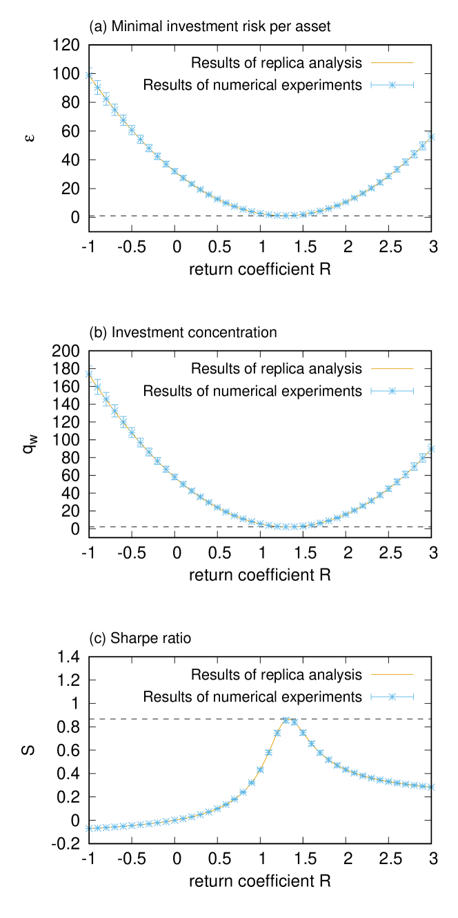
Figure 1: Results of the replica analysis and the numerical experiments ($\alpha=p/N=2$). The horizontal axis indicates the return coefficient $R$, and the vertical axes show (a) the minimal investment risk per asset $\varepsilon$, (b) the investment concentration $q_{w}$, and (c) the Sharpe ratio $S$. The solid (orange) lines indicate the results of the replica analysis for (a) Eq. (36), (b) Eq. (30), and (c) Eq. (37). The (blue) asterisks with error bars indicate the results of the numerical simulation, and the dashed (black) lines indicate the results for (a) $\varepsilon_{0}=\frac{\alpha-1}{2\left\langle v^{-1}\right\rangle}$, (b) $\frac{1}{\alpha-1}+\frac{\left\langle v^{-2}\right\rangle}{\left\langle v^{-1}\right\rangle^{2}}$, and (c) $S(R^{*})=\sqrt{\frac{\left\langle v^{-1}r^{2}\right\rangle}{\alpha-1}}$.

VI Conclusion and future work

To refine the portfolio optimization problem discussed in previous work Shinzato-2016-PRE11 , which was under constraints of budget and expected return for the case that the variance of the return rate of each asset is unique and the hyperparameters of the means of the assets are independently and identically Gaussian distributed, in the present study we consider the portfolio optimization problem under these two constraints for the case that the hyperparameters of the means and variances of the assets have arbitrary distributions (although, so as to verify our proposed method, the distributions of hyperparameters were limited in numerical simulations). Using replica analysis, the minimal investment risk per asset, investment concentration, and Sharpe ratio of the above-explained optimization problem were analytically derived. Moreover, by comparing the results obtained in previous work, those derived using the Lagrange multiplier method, and our numerical results, the applicability of our proposed approach based on replica analysis was validated. In addition, relations between macroscopic variables which are represented by the Pythagorean theorem of the Sharpe ratio in Eq. (64) and the two opportunity losses in Eqs. (70) and (73) were derived. Furthermore, it was shown that the portfolio which is discussed in operations research and which can minimize the expected investment risk (which is not the same as the investment risk itself) is not always consistent with the optimal portfolio which can minimize the investment risk. Since the above opportunity losses are larger than 1, from the argument in this paper, as the unfortunate consequence, it is validated that the approach which should be based on an ill-developed philosophy is not possible to attain the optimal asset management which is expected by the rational investors. While, fortunately, interdisciplinary research fields have provided step-by-step richer knowledge and novel insight for optimal investing to rational investors using the analytical approaches well-developed in statistical mechanical informatics, we should continue ongoing work to further explore the undeveloped frontier in order to develop an approach which can derive the optimal investment management which meets the expectations of investors.

As future work, although the present paper does not discuss mathematically our obtained relation between the macroscopic variables sufficiently, in order to increase the sophistication of the body of knowledge of mathematical finance, we need to provide a geometrical interpretation of the Pythagorean theorem of the Sharpe ratio. Moreover, we also need to determine additional relations between the macroscopic variables besides the Pythagorean theorem of the Sharpe ratio in Eq. (64) and the opportunity losses in (70) and (73).

Appendix A Replica calculation

In this appendix, we explain replica analysis in the main context of interest in this paper. The same as in previous work Shinzato-2015-PLOS7 ; Shinzato-ve-fixed2016 ; Shinzato-2017-JSTAT2 ; Shinzato-2016-PRE11 ; Shinzato-2016-PRE12 , $E\left[Z^{n}(R,X,\vec{r})\right],(n\in{\bf Z})$ is described as follows:

$$E\left[Z^{n}(R,X,\vec{r})\right]$$ (82)

$$= \mathop{\rm Extr}_{\vec{k},\vec{\theta}}\frac{1}{(2\pi)^{\frac{Nn}{2}+pn}}\int_{-\infty}^{\infty}\prod_{a}d\vec{w}_{a}d\vec{u}_{a}d\vec{z}_{a}$$

$$E\left[\exp\left(-\frac{\beta}{2}\sum_{\mu,a}z_{\mu a}^{2}\right.\right.+\sum_{a}k_{a}\left(\sum_{i}w_{ia}-N\right)$$

$$+\sum_{a}\theta_{a}\left(\sum_{i}r_{i}w_{ia}-NR\right)$$

$$\left.\left.+i\sum_{\mu,a}u_{\mu a}\left(z_{\mu a}-\frac{1}{\sqrt{N}}\sum_{i}w_{ia}x_{i\mu}\right)\right)\right],$$

where here for convenience, $\sum_{i}$ indicates $\sum_{i=1}^{N}$, $\sum_{\mu}$ represents $\sum_{\mu=1}^{p}$, $\sum_{a}$ is $\sum_{a=1}^{n}$, and $\prod_{a}$ means $\prod_{a=1}^{n}$. Moreover, $\vec{w}_{a}=(w_{1a},w_{2a},\cdots,w_{Na})^{\rm T}\in{\bf R}^{N},(a,b=1,2,\cdots,n)$, $\vec{u}_{a}=(u_{1a},u_{2a},\cdots,u_{pa})^{\rm T}\in{\bf R}^{p}$, $\vec{z}_{a}=(z_{1a},z_{2a},\cdots,z_{pa})^{\rm T}\in{\bf R}^{p}$, $\vec{k}=(k_{1},k_{2},\cdots,k_{n})^{\rm T}\in{\bf R}^{n}$, and $\vec{\theta}=(\theta_{1},\theta_{2},\cdots,\theta_{n})^{\rm T}\in{\bf R}^{n}$. Further, the integral $g(\vec{w}_{a})$ over the feasible portfolio subset space (that is, satisfying the budget constraint in Eq. (1) and the expected return constraint in Eq. (2)), ${\cal W}$, is approximated as follows:

$$\int_{\vec{w}_{a}\in{\cal W}}d\vec{w}_{a}g(\vec{w}_{a})$$

$$= \mathop{\rm Extr}_{k_{a},\theta_{a}}\frac{1}{(2\pi)^{\frac{N}{2}}}\int_{-\infty}^{\infty}d\vec{w}_{a}g(\vec{w}_{a})$$

$$\exp\left(k_{a}\left(\sum_{i}w_{ia}-N\right)+\theta_{a}\left(\sum_{i}r_{i}w_{ia}-N\right)\right).$$

Next, we can assess each part of the integral step by step as follows:

$$\log E\left[\exp\left(-\frac{i}{\sqrt{N}}\sum_{i,\mu}x_{i\mu}\sum_{a}u_{\mu a}w_{ia}\right)\right]$$ (84)

$$= \mathop{\rm Extr}_{Q_{w},\tilde{Q}_{w},Q_{s},\tilde{Q}_{s}}\left\{-\frac{1}{2}\sum_{\mu,a,b}q_{sab}u_{\mu a}u_{\mu b}\right.$$

$$-\frac{1}{2}\sum_{a,b}\tilde{q}_{wab}\left(\sum_{i}w_{ia}w_{ib}-Nq_{wab}\right)$$

$$\left.-\frac{1}{2}\sum_{a,b}\tilde{q}_{sab}\left(\sum_{i}v_{i}w_{ia}w_{ib}-Nq_{sab}\right)\right\}.$$

As the order parameters, we define

$$q_{wab} = \frac{1}{N}\sum_{i=1}^{N}w_{ia}w_{ib},$$ (85)

$$q_{sab} = \frac{1}{N}\sum_{i=1}^{N}v_{i}w_{ia}w_{ib},$$ (86)

and $\tilde{q}_{wab}$ and $\tilde{q}_{sab}$ are the corresponding auxiliary parameters. Moreover, $Q_{w}=\left\{q_{wab}\right\}\in{\bf R}^{n\times n}$, $Q_{s}=\left\{q_{sab}\right\}\in{\bf R}^{n\times n}$, $\tilde{Q}_{w}=\left\{\tilde{q}_{wab}\right\}\in{\bf R}^{n\times n}$, and $\tilde{Q}_{s}=\left\{\tilde{q}_{sab}\right\}\in{\bf R}^{n\times n}$ are used. In addition, using the Gaussian integral with respect to $\vec{u}_{a},\vec{z}_{a}$,

$$\frac{1}{(2\pi)^{pn}}\int_{-\infty}^{\infty}\prod_{a}d\vec{u}_{a}d\vec{z}_{a}\exp\left(-\frac{\beta}{2}\sum_{\mu,a}z_{\mu a}^{2}\right.$$ (87)

$$\left.+i\sum_{\mu,a}u_{\mu a}z_{\mu a}-\frac{1}{2}\sum_{\mu,a,b}q_{sab}u_{\mu a}u_{\mu b}\right)$$

$$= \exp\left(-\frac{p}{2}\log\det\left|I+\beta Q_{s}\right|\right),$$

where $I$ is the ${n\times n}$ identify matrix. In a similar way, using the Gaussian integral with respect to $\vec{w}_{a}$,

$$\frac{1}{(2\pi)^{\frac{Nn}{2}}}\int_{-\infty}^{\infty}\prod_{a}d\vec{w}_{a}\exp\left(-\frac{1}{2}\sum_{i,a,b}\tilde{q}_{wab}w_{ia}w_{ib}\right.$$ (88)

$$\left.-\frac{1}{2}\sum_{i,a,b}\tilde{q}_{sab}v_{i}w_{ia}w_{ib}+\sum_{i,a}k_{a}w_{ia}+\sum_{i,a}\theta_{a}r_{i}w_{ia}\right)$$

$$= \exp\left(-\frac{1}{2}\sum_{i}\log\det\left|\tilde{Q}_{w}+v_{i}\tilde{Q}_{s}\right|\right.$$

$$\left.+\frac{1}{2}\sum_{i}(\vec{k}+r_{i}\vec{\theta})^{\rm T}\left(\tilde{Q}_{w}+v_{i}\tilde{Q}_{s}\right)^{-1}(\vec{k}+r_{i}\vec{\theta})\right).$$

From this,

$$\log E\left[Z^{n}(R,X,\vec{r})\right]$$ (89)

$$= \mathop{\rm Extr}_{\vec{k},\vec{\theta},Q_{w},\tilde{Q}_{w},Q_{s},\tilde{Q}_{s}}\left\{\frac{N}{2}\sum_{a,b}q_{wab}\tilde{q}_{wab}+\frac{N}{2}\sum_{a,b}q_{sab}\tilde{q}_{sab}\right.$$

$$-N\sum_{a}k_{a}-NR\sum_{a}\theta_{a}-\frac{p}{2}\log\det\left|I+\beta Q_{s}\right|$$

$$-\frac{1}{2}\sum_{i}\log\det\left|\tilde{Q}_{w}+v_{i}\tilde{Q}_{s}\right|$$

$$\left.+\frac{1}{2}\sum_{i}(\vec{k}+r_{i}\vec{\theta})^{\rm T}\left(\tilde{Q}_{w}+v_{i}\tilde{Q}_{s}\right)^{-1}(\vec{k}+r_{i}\vec{\theta})\right\}.$$

and, in the limit of a large number of assets, using the replica symmetric solution derived in Eqs. (13) to (24),

$$\lim_{N\to\infty}\frac{1}{N}\log E\left[Z^{n}(R,X,\vec{r})\right]$$ (90)

$$= \mathop{\rm Extr}_{\Theta}\left\{\frac{n}{2}(\chi_{w}+q_{w})(\tilde{\chi}_{w}-\tilde{q}_{w})-\frac{n(n-1)}{2}q_{w}\tilde{q}_{w}\right.$$

$$+\frac{n}{2}(\chi_{s}+q_{s})(\tilde{\chi}_{s}-\tilde{q}_{s})-\frac{n(n-1)}{2}q_{s}\tilde{q}_{s}-nk-nR\theta$$

$$-\frac{\alpha(n-1)}{2}\log(1+\beta\chi_{s})-\frac{\alpha}{2}\log(1+\beta\chi_{s}+n\beta q_{s})$$

$$-\frac{n-1}{2}\left\langle\log(\tilde{\chi}_{w}+v\tilde{\chi}_{s})\right\rangle$$

$$-\frac{1}{2}\left\langle\log(\tilde{\chi}_{w}+v\tilde{\chi}_{s}-n(\tilde{q}_{w}+v\tilde{q}_{s}))\right\rangle$$

$$\left.+\frac{n}{2}\left\langle\frac{(k+r\theta)^{2}}{\tilde{\chi}_{w}+v\tilde{\chi}_{s}-n(\tilde{q}_{w}+v\tilde{q}_{s})}\right\rangle\right\}$$

can be calculated. Substituting the result into Eq. (9), Eq. (25) is obtained by using $\alpha=p/N\sim O(1)$.

By a similar argument, we can easily solve the dual problem in subsection IV.2 by using replica analysis. From the discussion in previous work Shinzato-2016-PRE11 , the partition function $Z(\varepsilon,X,\vec{r})$ and the Hamiltonian ${\cal H}^{\prime}(\vec{w}|\vec{r})$ are defined as follows:

$$Z(\varepsilon,X,\vec{r}) = \int_{\vec{w}\in{\cal W}^{\prime}}d\vec{w}e^{\beta{\cal H}^{\prime}(\vec{w}|\vec{r})},$$ (91)

$${\cal H}^{\prime}(\vec{w}|\vec{r}) = \sum_{i=1}^{N}r_{i}w_{i},$$ (92)

where the feasible portfolio subset space characterized by the constraints of budget and investment risk,

$${\cal W}^{\prime} = \left\{\vec{w}\in{\bf R}^{N}\left|\vec{w}^{\rm T}\vec{e}=N,N\varepsilon=\frac{1}{2}\vec{w}^{\rm T}J\vec{w}\right.\right\},\qquad$$ (93)

is employed. From this, using the self-averaging property of this disordered system, in order to perform this optimization problem,

$$\phi = \lim_{N\to\infty}\frac{1}{N}E\left[\log Z(\varepsilon,X,\vec{r})\right],$$ (94)

is defined. Then, from the following identical equations,

$$R^{\max} = \lim_{\beta\to\infty}\frac{\partial\phi}{\partial\beta},$$ (95)

$$R^{\min} = \lim_{\beta\to-\infty}\frac{\partial\phi}{\partial\beta},$$ (96)

the maximal and minimal expected returns per asset, $R^{\max}$ and $R^{\min}$, can be evaluated.

In a similar way to the above-discussed replica analysis, using the replica symmetric solution,

$$\phi = \mathop{\rm Extr}_{\Theta}\left\{\varepsilon\theta-k-\frac{\alpha}{2}\log(1+\theta\chi_{s})-\frac{\alpha\theta q_{s}}{2(1+\theta\chi_{s})}\right.$$ (97)

$$+\frac{1}{2}(\chi_{w}+q_{w})(\tilde{\chi}_{w}-\tilde{q}_{w})+\frac{1}{2}q_{w}\tilde{q}_{w}$$

$$+\frac{1}{2}(\chi_{s}+q_{s})(\tilde{\chi}_{s}-\tilde{q}_{s})+\frac{1}{2}q_{s}\tilde{q}_{s}+\frac{1}{2}\left\langle\frac{\tilde{q}_{w}+v\tilde{q}_{s}}{\tilde{\chi}_{w}+v\tilde{\chi}_{s}}\right\rangle$$

$$\left.-\frac{1}{2}\left\langle\log(\tilde{\chi}_{w}+v\tilde{\chi}_{s})\right\rangle+\frac{1}{2}\left\langle\frac{(k+r\beta)^{2}}{\tilde{\chi}_{w}+v\tilde{\chi}_{s}}\right\rangle\right\},$$

can also be estimated where $\Theta=\left\{k,\theta,\chi_{w},q_{w},\tilde{\chi}_{w},\tilde{q}_{w},\chi_{s},q_{s},\tilde{\chi}_{s},\tilde{q}_{s}\right\}$ is the set of the order parameters. From the extremum conditions for Eq. (97) with respect to these parameters, in terms of parameter $\theta$, the primal parameters are as follows:

$$\chi_{s} = \frac{1}{\theta(\alpha-1)},$$ (98)

$$q_{s} = \frac{\alpha}{(\alpha-1)\left\langle v^{-1}\right\rangle}+\frac{\alpha\left\langle v^{-1}\right\rangle V_{1}}{(\alpha-1)^{3}}\left(\frac{\beta}{\theta}\right)^{2},$$ (99)

$$k = \frac{\theta(\alpha-1)}{\left\langle v^{-1}\right\rangle}-\beta R_{1}.$$ (100)

Furthermore,

$$\frac{\partial\phi}{\partial\beta} = \frac{\beta\left\langle v^{-1}r^{2}\right\rangle}{\theta(\alpha-1)}+\frac{k\left\langle v^{-1}r\right\rangle}{\theta(\alpha-1)}$$ (101)

$$= R_{1}+\frac{\left\langle v^{-1}\right\rangle V_{1}}{\alpha-1}\frac{\beta}{\theta},$$

is obtained. Then in order to analyze the upper and lower bounds of the expected return per asset, we need to assess $\theta$, which needs to satisfy the following equation:

$$\varepsilon = \frac{\alpha\chi_{s}}{2(1+\theta\chi_{s})}+\frac{\alpha q_{s}}{2(1+\theta\chi_{s})^{2}}$$ (102)

$$= \frac{1}{2\theta}+\frac{\alpha-1}{2\left\langle v^{-1}\right\rangle}+\frac{\left\langle v^{-1}\right\rangle V_{1}}{2(\alpha-1)}\left(\frac{\beta}{\theta}\right)^{2}.$$

Rearranging, this can be written as

$$\left(\frac{\beta}{\theta}\right)^{2} = \frac{2(\alpha-1)}{\left\langle v^{-1}\right\rangle V_{1}}\left(\varepsilon-\frac{1}{2\theta}-\frac{\alpha-1}{2\left\langle v^{-1}\right\rangle}\right).$$ (103)

Considering the limit as $\left|\beta\right|\to\infty$, we assume $\beta/\theta\sim O(1)$; then

$$\frac{\beta}{\theta} = \pm\frac{\alpha-1}{\left\langle v^{-1}\right\rangle}\sqrt{\frac{1}{V_{1}}\left(\frac{2\left\langle v^{-1}\right\rangle}{\alpha-1}\varepsilon-1\right)}.$$ (104)

Note that for $\beta\to\infty$, the right-hand side must be positive, whereas if $\beta\to-\infty$, it must be negative. Substituting this expression into Eq. (101), we obtain

$$\lim_{|\beta|\to\infty}\frac{\partial\phi}{\partial\beta} = \left\{\begin{array}[]{ll}R_{1}+\sqrt{V_{1}\left(\frac{2\left\langle v^{-1}\right\rangle}{\alpha-1}\varepsilon-1\right)}&\beta\to\infty\\ R_{1}-\sqrt{V_{1}\left(\frac{2\left\langle v^{-1}\right\rangle}{\alpha-1}\varepsilon-1\right)}&\beta\to-\infty\end{array}\right..$$ (107)

Thus, $R^{\max}$ and $R^{\min}$ are consistent with Eqs. (53) and (54).

Appendix B Replica analysis for moments

Here $\frac{1}{N}\vec{e}^{\rm T}J^{-1}\vec{e},\frac{1}{N}\vec{r}^{\rm T}J^{-1}\vec{e},$ and $\frac{1}{N}\vec{r}^{\rm T}J^{-1}\vec{r}$ are analyzed. First, in order to determine them, the partition function $Z(k,\theta,X)$ is defined as follows:

$$Z(k,\theta,X) = \frac{1}{(2\pi)^{\frac{N}{2}}}\int_{-\infty}^{\infty}d\vec{w}e^{-\frac{1}{2}\vec{w}^{\rm T}J\vec{w}+\vec{w}^{\rm T}(k\vec{e}+\theta\vec{r})},\qquad$$ (109)

where $J=XX^{\rm T}\in{\bf R}^{N\times N}$. The partition function is calculated using

$$\log Z(k,\theta,X) = \frac{1}{2}\log\det|J|+\frac{k^{2}}{2}\vec{e}^{\rm T}J^{-1}\vec{e}+\frac{\theta^{2}}{2}\vec{r}^{\rm T}J^{-1}\vec{r}$$ (110)

$$+k\theta\vec{r}^{\rm T}J^{-1}\vec{e}.$$

From the self-averaging property, in the limit of large $N$,

$$\phi(k,\theta) = \lim_{N\to\infty}\frac{1}{N}E\left[\log Z(k,\theta,X)\right],$$ (111)

from the second derivatives of $\phi$ with respect to $k,\theta$, the typical behaviors of $\frac{1}{N}\vec{e}^{\rm T}J^{-1}\vec{e},\frac{1}{N}\vec{r}^{\rm T}J^{-1}\vec{e}$, and $\frac{1}{N}\vec{r}^{\rm T}J^{-1}\vec{r}$ are easily determined. Here, using replica analysis and the replica symmetric solution in the limit that the number of assets $N$ is large,

$$\phi(k,\theta) = \mathop{\rm Extr}_{\chi_{s},q_{s},\tilde{\chi}_{s},\tilde{q}_{s}}\left\{\frac{1}{2}(\chi_{s}+q_{s})(\tilde{\chi}_{s}-\tilde{q}_{s})+\frac{q_{s}\tilde{q}_{s}}{2}\right.$$ (112)

$$-\frac{\alpha}{2}\log(1+\chi_{s})-\frac{\alpha q_{s}}{2(1+\chi_{s})}-\frac{1}{2}\left\langle\log v\right\rangle$$

$$\left.-\frac{1}{2}\log\tilde{\chi}_{s}+\frac{\tilde{q}_{s}}{2\tilde{\chi}_{s}}+\frac{1}{2\tilde{\chi}_{s}}\left\langle\frac{(k+r\theta)^{2}}{v}\right\rangle\right\},\qquad$$

is obtained. From the extremum conditions for Eq. (112),

$$\chi_{s} = \frac{1}{\alpha-1},$$ (113)

$$q_{s} = \frac{\alpha}{(\alpha-1)^{3}}\left\langle\frac{(k+r\theta)^{2}}{v}\right\rangle,$$ (114)

$$\tilde{\chi}_{s} = \alpha-1,$$ (115)

$$\tilde{q}_{s} = \frac{1}{\alpha-1}\left\langle\frac{(k+r\theta)^{2}}{v}\right\rangle,$$ (116)

are obtained by using the replica symmetric solution in Eqs. (16) and (22). Plugging these into Eq. (112),

$$\phi(k,\theta) = \frac{1}{2}-\frac{\alpha}{2}\log\frac{\alpha}{\alpha-1}-\frac{1}{2}\log(\alpha-1)$$ (117)

$$-\frac{1}{2}\left\langle\log v\right\rangle+\frac{1}{2(\alpha-1)}\left\langle\frac{(k+r\theta)^{2}}{v}\right\rangle,$$

is obtained. Thus, $\frac{1}{N}\vec{e}^{\rm T}J^{-1}\vec{e},\frac{1}{N}\vec{r}^{\rm T}J^{-1}\vec{e},$ and $\frac{1}{N}\vec{r}^{\rm T}J^{-1}\vec{r}$ are calculated as follows:

$$\lim_{N\to\infty}\frac{1}{N}\vec{e}^{\rm T}J^{-1}\vec{e} = \frac{\partial^{2}\phi(k,\theta)}{\partial k^{2}}$$ (118)

$$= \frac{\left\langle v^{-1}\right\rangle}{\alpha-1},$$

$$\lim_{N\to\infty}\frac{1}{N}\vec{r}^{\rm T}J^{-1}\vec{e} = \frac{\partial^{2}\phi(k,\theta)}{\partial\theta\partial k}$$ (119)

$$= \frac{\left\langle v^{-1}r\right\rangle}{\alpha-1},$$

$$\lim_{N\to\infty}\frac{1}{N}\vec{r}^{\rm T}J^{-1}\vec{r} = \frac{\partial^{2}\phi(k,\theta)}{\partial\theta^{2}}$$ (120)

$$= \frac{\left\langle v^{-1}r^{2}\right\rangle}{\alpha-1}.$$

Appendix C Stochastic Optimization

In this appendix, we summarize the framework of stochastic optimization Shinzato-2015-PLOS7 . First, for a given random variable $X$, using a real-valued function bounded below with respect to the control parameter $w\in{\cal W}$, $f(w,X)$, we discuss the optimal solution $w$ which can minimize $f(w,X)$, the minimal value of $f(w,X)$, and its typical behavior. The random variable $X$ is assumed to follow one of the well-known distributions and the feasible subset space of the control parameter $w$ is ${\cal W}$. From the below discussion, the following results do not always require that $f(w,X)$ is convex with respect to $w$.

For a pair $w,X$,

$$f(w,X)\geq\mathop{\min}_{w\in{\cal W}}f(w,X),$$ (121)

holds. Let $w^{*}(X)$ be the value of $w$ which realizes the minimum on the right-hand side, that is,

$$w^{*}(X) = \arg\mathop{\min}_{w\in{\cal W}}f(w,X).$$ (122)

Thus, the equality case of Eq. (121) can be rewritten as follows:

$$f(w^{*}(X),X) = \mathop{\min}_{w\in{\cal W}}f(w,X),$$ (123)

that is,

$$f(w,X)\geq f(w^{*}(X),X),$$ (124)

in which one should note that the optimal solution $w^{*}(X)$ depends on random variable $X$, as indicated by the notation.

Next we can take the expectation of both sides of Eq. (124) with respect to random variable $X$:

$$E_{X}[f(w,X)]\geq E_{X}[f(w^{*}(X),X)].$$ (125)

Since the right-hand side of Eq. (125) is constant and the left-hand side holds for any control parameter $w\in{\cal W}$, the following inequality holds:

$$\mathop{\min}_{w\in{\cal W}}E_{X}[f(w,X)]\geq E_{X}\left[f(w^{*}(X),X)\right].$$ (126)

We can substitute Eq. (123) into this right-hand side to also obtain

$$\mathop{\min}_{w\in{\cal W}}E_{X}[f(w,X)]\geq E_{X}\left[\mathop{\min}_{w\in{\cal W}}f(w,X)\right].$$ (127)

Thus, the minimum of the expectation of $f(w,X)$ with respect to control parameter $w$, $\mathop{\min}_{w\in{\cal W}}E_{X}[f(w,X)]$, is not always less than the expectation of the minimum of $f(w,X)$ with respect to $w$, $E_{X}\left[\mathop{\min}_{w\in{\cal W}}f(w,X)\right]$. Further, by a similar argument, we can also consider the maximization of a real-valued function bounded above with respect to $w$, $g(w,X)$, and obtain

$$\mathop{\max}_{w\in{\cal W}}E_{X}[g(w,X)]\leq E_{X}\left[\mathop{\max}_{w\in{\cal W}}g(w,X)\right].$$ (128)

Returning to the minimization problem, suppose $\mathop{\min}_{w\in{\cal W}}f(w,X)$ satisfies the following self-averaging property:

$$\mathop{\min}_{w\in{\cal W}}f(w,X) = E_{X}\left[\mathop{\min}_{w\in{\cal W}}f(w,X)\right].$$ (129)

Then from Eqs. (127) and (129),

$$\mathop{\min}_{w\in{\cal W}}E_{X}[f(w,X)]\geq\mathop{\min}_{w\in{\cal W}}f(w,X),$$ (130)

which was discussed in Ref. Shinzato-2015-PLOS7 . That is, in terms of the discussion in the main text, control parameter $w$ is a portfolio, random variable $X$ is a return rate matrix, real-valued function $f(w,X)$ bounded from below is the investment risk, and the feasible subset space ${\cal W}$ corresponds to several constraints on the portfolio. Thus, the discussion here clarifies that the ordinary portfolio which can minimize the expected investment risk discussed in operations research, $w^{\rm OR}=\arg\mathop{\min}_{w\in{\cal W}}E_{X}[f(w,X)]$, is not always consistent with the optimal portfolio which can minimize the investment risk, $w^{*}(X)=\arg\mathop{\min}_{w\in{\cal W}}f(w,X)$, and which is sought by rational investors. Namely, as a physical interpretation of Eq. (130), the left-hand side of Eq. (130) corresponds to an annealed disordered system and the right-hand side of Eq. (130) is related to a quenched disordered system. Moreover, in previous work Shinzato-2015-PLOS7 , it was verified that the minimal investment risk per asset $\varepsilon$ and its investment concentration $q_{w}$ (and Sharpe ratio $S$, which is defined using the minimal investment risk per asset $\varepsilon$ and the expected return coefficient $R$) satisfy the self-averaging property.

References

- (1) H. Markowitz, Portfolio selection, J. Fin. 7, 77 (1952).
- (2) H. Markowitz, Portfolio Selection: Efficient Diversification of Investments (J. Wiley & Sons, New York, 1959).
- (3) Z. Bodie, A. Kane and A. J. Marcus, Investments (McGraw-Hill, New York, 2014).
- (4) D. G. Luenberger, Investment Science (Oxford University Press, Oxford, 1997).
- (5) J. -L. Prigent, Portfolio Optimization and Performance Analysis (Chapman and Hall/CRC, 2007).
- (6) A. Ang, Asset Management (Oxford University Press, 2014).
- (7) J. C. Francis and D. Kim, Modern Portfolio Theory (J. Wiley & Sons, New York , 2013).
- (8) E. J. Elton M. J. Gruber, S. J. Brown, and W. N. Goetzmann, Modern Portfolio Theory and Investment Analysis (J. Wiley & Sons, New York , 2014).
- (9) S. Ciliberti and M. Mzard, Risk minimization through portfolio replication, Eur. Phys. J. B, 27, 175 (2007).
- (10) S. Ciliberti, I. Kondor, and M. Mzard, On the feasibility of portfolio optimization under expected shortfall, Quant. Fin., 7, 389 (2007).
- (11) F. Caccioli, S. Still, M. Marsili, and I. Kondor, Optimal liquidation strategies regularize portfolio selection , Euro. J. Fin. 19, 554 (2013).
- (12) S. Pafka and I. Kondor, Noisy covariance matrices and portfolio optimization II, Physica A, 319, 487 (2003).
- (13) T. Shinzato, Self-averaging property of minimal investment risk of mean-variance model, PLoS One, 10, e0133846 (2015).
- (14) T. Shinzato and M. Yasuda, Belief propagation algorithm for portfolio optimization problems, PLoS One, 10, e0134968 (2015).
- (15) T. Shinzato, Portfolio optimization problem with nonidentical variances of asset returns using statistical mechanical informatics, Phys. Rev. E, 94, 062102 (2016).
- (16) T. Shinzato, Statistical Mechanical Informatics for Portfolio Optimization Problems without Short Selling , Tech. Rep. IEICE, 110(461), 23 (2011).
- (17) I. Kondor, G. Papp, and F. Caccioli, Analytic solution to variance optimization with no short-selling, arxiv.org/abs/1612.07067 (2016).
- (18) T. Shinzato, Minimal investment risk of portfolio optimization problem with budget and investment concentration constraints, J. Stat. Mech. 023301 (2017).
- (19) T. Shinzato, Maximizing and minimizing investment concentration with constraints of budget and investment risk, arxiv.org/abs/1608.04522 (2016).
- (20) T. Shinzato, Replica analysis for the duality of the portfolio optimization problem, Phys. Rev. E, 94, 052307 (2016).
- (21) I. Varga-Haszonits, F. Caccioli, and I. Kondor, Replica approach to mean-variance portfolio optimization, J. Stat. Mech. 123404 (2016).
- (22) I. B. Aban, M. M. Meerschaert and A. K. Panorska, Parameter estimation for the truncated Pareto distribution, J. Amer. Stat. Asso. 101, 270 (2012).