Lindblad approach to spatio-temporal quantum dynamics
of phonon-induced carrier capture processes

Abstract

In view of the ultrashort spatial and temporal scales involved, carrier capture processes in nanostructures are genuine quantum phenomena. To describe such processes, methods with different levels of approximations have been developed. By properly tailoring the Lindblad-based nonlinear single-particle density matrix equation provided by an alternative Markov approach, in this work we present a Lindblad superoperator to describe how the phonon-induced carrier capture affects the spatio-temporal quantum dynamics of a flying wave packet impinging on a quantum dot. We compare the results with non-Markovian quantum kinetics calculations and discuss the advantages and drawbacks of the two approaches.

I Introduction

The shrinking of space- and time-scales of modern devices has reached the threshold where semiclassical approaches like the Boltzmann equation Jacoboni and Lugli (1989) are no longer able to fully catch the genuine quantum mechanical effects on the electronic transport Rossi and Kuhn (2002); Axt and Kuhn (2004); Pecchia and Di Carlo (2004). To model the dynamics in these systems, several quantum mechanical approaches have been proposed, including nonequilibrium Green’s functions Haug and Koch (2004); Bonitz (1998); Datta (1997), path integrals Makri and Makarov (1995); Vagov et al. (2011); Glässl et al. (2011), surface hopping approaches Wang et al. (2015, 2016) and density matrix based treatments either on a non-Markovian, quantum kinetic (QK) level Schilp et al. (1994); Rossi and Kuhn (2002); Axt and Kuhn (2004) or on a Markovian level Fischetti (1999); Knezevic (2008); Hohenester and Pötz (1997); Bi Sun and Milburn (1999).

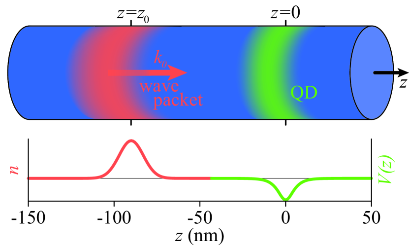
Figure 1: (Color online) Schematic representation of the carrier capture process from a wave packet (red shapes) traveling in a cylindrical quantum wire into an embedded QD (green shapes): the upper and lower panels show the process in three-dimensional space and reduced to the longitudinal direction $z$, respectively. Here $z_{0}$ and $k_{0}$ are the initial central position and wave vector of the wave packet, respectively (see also Eq. (10)).

Carrier capture processes into localized states of a nanostructure Ferreira and Bastard (2015); Glanemann et al. (2005); Reiter et al. (2006) are within the most intrinsically quantum mechanical processes, as can be inferred both from the nanometric size of its constituents and the subpicosecond time-scale of the interaction. Furthermore, they involve transitions from extended states in the continuous part of the spectrum into localized states in the discrete part. In this work we focus on a wave packet traveling in a quantum wire (QWR) which, when passing by a quantum dot (QD) embedded in the wire, interacts with the latter by means of electron-phonon scattering, see Fig. 1. Experimentally, QWRs with an embedded QD have been obtained in different geometries, e.g., by cleaved-edge overgrowth Wegscheider et al. (1997), by growth on a patterned substrate Lienau et al. (2000) or by growth in vertical nanowires Tatebayashi et al. (2015); Heiss et al. (2013); Claudon et al. (2010); Loitsch et al. (2015).

The intrinsically spatially inhomogeneous problem induces, in turn, a nontrivial spatio-temporal dynamics, which could then suggest interesting applications in electronic-based quantum information processing. For example, in the concept of flying qubits one could use the shape of a traveling electronic wave packet to store and transmit information around the nanodevice Bertoni et al. (2000); Ionicioiu et al. (2001); Fève et al. (2007). Potentially, the carrier capture processes could be able to alter this information in a point which is strongly localized both in space and time Glanemann et al. (2005); considering the rise of novel materials able to provide strain-tunable QDs Feng et al. (2012); Manzeli et al. (2015); Roldán et al. (2015); Kern et al. (2016) or dispersionless propagation Rosati et al. (2015, 2015), this property could make the capture processes one key ingredient of electronic-based quantum information protocols.

On the other hand, due to the intrinsically local nature of the carrier-phonon interaction in combination with the nonlocal character of the continuum states, the spatio-temporal dynamics of carrier capture processes is extremely demanding to describe on a fully quantum-mechanical level. In view of their importance for hetero-structure semiconductor lasers, capture rates obtained from Fermi’s Golden Rule (FGR) have been calculated for many years, first mainly for the capture from bulk into quantum well states Brum and Bastard (1986); Kuhn and Mahler (1989); Preisel and Mo/rk (1994); Reiter et al. (2009) and then also for the capture into QD states Ferreira and Bastard (1999); Magnusdottir et al. (2003); Nielsen et al. (2004). The resulting semiclassical treatments may thus efficiently provide the total captured charge, however they will typically not be able to properly describe the spatio-temporal dynamics of the traveling wave packet. In addition, the different effective dimensionalities of states involved in capture processes give rise to difficulties already in properly defining the semiclassical equation: in fact, the scattering rates typically depend on the normalization volume of the delocalized states,which then has to be fixed by some more or less rigorous argument.

This difficulty in describing spatio-temporal dynamics together with scattering processes is related to the fact that, as long as only occupations are considered, as is often done in these calculations, the electrons that occupy continuum states are always completely delocalized. Space dependencies are then often introduced in a phenomenological, parametric way. However, spatially inhomogeneous distributions, where the carriers are not completely delocalized, require superpositions of these states, i.e., off-diagonal elements in the density matrices defined with respect to these states Herbst et al. (2003); Steininger et al. (1996). This is exactly what has been done in QK studies, where it has been shown that the interaction provides local capture dynamics, in contrast to what would be seen within a diagonal description Glanemann et al. (2005); Reiter et al. (2006, 2007). A local interaction in space translates into a finite duration in time, which in turn induces broadened energy selection rules with respect to the Dirac-delta of conventional FGR Glanemann et al. (2005); Reiter et al. (2006). QK treatments provide accurate predictions, but their computational costs make it complicated to study longer evolutions or stronger interaction mechanisms, where in addition numerical instabilities, especially on longer time scales, may appear. They also often prohibit the extension to more complicated structures, e.g., higher-dimensional systems which cannot be reduced by spatial symmetries.

Hence it is desirable to have a computationally lighter approach still capable of describing the spatio-temporal dynamics, thereby being intermediate between FGR and QK. We look therefore for an approach able to deal with non-diagonal density matrices through a closed equation of motion: Conventional Markov approximations Fischetti (1999); Knezevic (2008); Hohenester and Pötz (1997); Bi Sun and Milburn (1999) could in principle fulfill these requirements, but the asymmetric shape of their superoperator may lead to huge instabilities due to their non-positive definite definition Rosati et al. (2014). The solution to the instability problem can be given by a recently introduced Markov approximation Taj et al. (2009), which in fact is able to provide a Lindblad-like many-body superoperator and a positive-definite nonlinear single-particle density matrix equation Rosati et al. (2014), the latter being of Lindblad type itself in the low density regime.

In this paper we extend this treatment to carrier-capture processes. We then compare the resulting Lindblad single-particle (LSP) approach to a full QK analysis, which can be considered as a benchmark. We show that the LSP approach catches the essential features of the spatio-temporal dynamics and further discuss the advantages and drawbacks of the two approaches.

The paper is organized as follows: In Sec. II we present the theory behind the carrier capture processes, recall the main fundamentals of the QK treatment and introduce the properly tailored LSP approach. In Sec. III we study the capture process of a nanometric flying wave packet impinging on a QD with one (Sec. III.1) or two (Sec. III.2) bound states, and finally conclude in Sec. IV.

II Theory

II.1 Hamiltonians and equations of motion

The starting point for our description is a proper definition of the single-particle eigenstates $|\alpha\rangle$ and the associated energy levels $\epsilon_{\alpha}$ corresponding to the nanodevice potential profile. We will reduce our system to be effectively one-dimensional by considering only the lowest transverse eigenmode of a cylindrical GaAs QWR with 100 nm² cross section. As a consequence, the state $|\alpha\rangle$ corresponds to the eigenfunction $\psi_{\alpha}(z)\equiv\langle z|\alpha\rangle$ solving the single-particle Schrödinger equation

$$\left[-\frac{\hbar^{2}}{2m^{*}}\frac{\partial^{2}}{\partial z^{2}}+V(z)\right]\psi_{\alpha}(z)=\epsilon_{\alpha}\psi_{\alpha}(z)\,,$$ (1)

with $m^{*}$ being the effective mass and $V(z)$ the profile of the QD potential along the longitudinal direction $z$ (see also Fig. 1). The single-particle spectrum is discrete for the bound states ($\epsilon_{\alpha}<0$) and continuous for the delocalized states ($\epsilon_{\alpha}>0$). The dynamical variable is the single-particle density operator $\hat{\rho}$, whose matrix elements $\rho_{\alpha\alpha^{\prime}}$ are defined as

$$\rho_{\alpha\alpha^{\prime}}=\mathrm{Tr}[\hat{c}_{\alpha^{\prime}}^{\dagger}\hat{c}_{\alpha}\boldsymbol{\hat{\rho}}]\,,$$ (2)

where $\hat{c}^{\dagger}_{\alpha}$ and $\hat{c}_{\alpha}$ are the creation and annihilation operators of state $\alpha$, while $\boldsymbol{\hat{\rho}}$ is the many-body density matrix containing all the electronic and phononic degrees of freedom. The dynamics of $\rho$ is given by

$$\begin{split}\frac{d\rho_{\alpha\alpha^{\prime}}}{dt}=&\mathrm{Tr}\left[\hat{c}_{\alpha^{\prime}}^{\dagger}\hat{c}_{\alpha}\frac{d\boldsymbol{\hat{\rho}}}{dt}\right]\\ \equiv&\left.\frac{d\rho_{\alpha\alpha^{\prime}}}{dt}\right|_{\text{free}}+\left.\frac{d\rho_{\alpha\alpha^{\prime}}}{dt}\right|_{\text{scat}}\,,\end{split}$$ (3)

where in the last equality we have distinguished between the scattering-free and electron-phonon induced dynamics, which are defined as

$$\left.\frac{d\rho_{\alpha\alpha^{\prime}}}{dt}\right|_{\text{free}} =\frac{1}{\imath\hbar}\mathrm{Tr}\left[\hat{c}_{\alpha^{\prime}}^{\dagger}\hat{c}_{\alpha}\left[\hat{H}_{\text{e}}+\hat{H}_{\text{ph}},\boldsymbol{\hat{\rho}}\right]\right],$$ (4a)

$$\left.\frac{d\rho_{\alpha\alpha^{\prime}}}{dt}\right|_{\text{scat}} =\frac{1}{\imath\hbar}\mathrm{Tr}\left[\hat{c}_{\alpha^{\prime}}^{\dagger}\hat{c}_{\alpha}\left[\hat{H}_{\text{e-ph}},\boldsymbol{\hat{\rho}}\right]\right]\,.$$ (4b)

The Hamiltonians $\hat{H}_{\text{e}}$ and $\hat{H}_{\text{ph}}$ appearing in Eq. (4a) are the scattering-free electronic and phononic Hamiltonians,

$$\hat{H}_{\text{e}}= \sum_{\alpha}\epsilon_{\alpha}\hat{c}^{\dagger}_{\alpha}\hat{c}_{\alpha}\quad,$$ (5)

$$\hat{H}_{\text{ph}}= \sum_{\xi}\hat{H}_{\xi}\equiv\sum_{\xi,\mathbf{q}}\hbar\omega^{\xi}_{\mathbf{q}}\hat{b}^{\xi\dagger}_{\mathbf{q}}\hat{b}^{\xi}_{\mathbf{q}}\,,$$ (6)

with $\xi$ denoting the type of phonon (e.g., optical or acoustic, longitudinal or transverse, …), $\mathbf{q}$ the three-dimensional phonon wave vector and $\hat{b}^{\xi\dagger}_{\mathbf{q}}$ ($\hat{b}^{\xi}_{\mathbf{q}}$) the creation (annihilation) operator of a phonon of type $\xi$ and wave vector $\mathbf{q}$.

The scattering-induced dynamics of Eq. (4b) is given by the electron-phonon Hamiltonian $\hat{H}_{\text{e-ph}}$. In a real-space representation the interaction Hamiltonian has the form

$$\hat{H}_{\text{e-ph}}=\int d^{3}r\hat{\Psi}^{\dagger}({\mathbf{r}})\hat{V}_{\text{e-ph}}({\mathbf{r}})\hat{\Psi}({\mathbf{r}})\,,$$ (7)

where $\hat{\Psi}^{\dagger}({\mathbf{r}})$ ($\hat{\Psi}({\mathbf{r}})$) are the creation (annihilation) operators for an electron at the position ${\mathbf{r}}$ and $\hat{V}_{\text{e-ph}}({\mathbf{r}})$ is the phonon-induced potential acting on the electrons. Its detailed form depends on the phonon type and the interaction mechanism (e.g., deformation potential, piezoelectric, polar optical, …). Equation (7) clearly shows that the interaction is local in space, i.e., it connects the annihilation of an electron at a given position with the creation at the same position. Inserting the mode representations of electrons and holes, the interaction Hamiltonian can be written in the more conventional form

$$\hat{H}_{\text{e-ph}}= \sum_{\xi}\hat{H}_{\text{e}-\xi}$$

$$= \sum_{\xi}\sum_{\alpha\alpha^{\prime},\mathbf{q}}(g^{\xi\mathbf{q}-}_{\alpha\alpha^{\prime}}\hat{c}^{\dagger}_{\alpha}\hat{c}_{\alpha^{\prime}}\hat{b}^{\xi}_{\mathbf{q}}+g^{\xi\mathbf{q}+}_{\alpha\alpha^{\prime}}\hat{c}^{\dagger}_{\alpha^{\prime}}\hat{c}_{\alpha}\hat{b}^{\xi\dagger}_{\mathbf{q}})\,,$$ (8)

with $+(-)$ standing for emission (absorption) of a phonon associated with a transition from state $\alpha$ to $\alpha^{\prime}$ ($\alpha^{\prime}$ to $\alpha$). Hereby we distinguish between continuous-continuous (CC, both $\alpha$ and $\alpha^{\prime}$ referring to delocalized states), discrete-discrete (DD, both $\alpha$ and $\alpha^{\prime}$ referring to bound states) and continuous-discrete transitions (CD, with one among $\alpha^{\prime}$ and $\alpha$ referring to a delocalized and the other to a bound state). In particular, the latter are responsible for the carrier capture processes. In view of the large energetic separation between the bottom of the delocalized states band and the bound states, the only phonons able to induce CD transitions are the optical ones. For the interaction matrix element we take the Fröhlich coupling which is typically the dominant electron-phonon interaction mechanism in III-V semiconductors. Therefore we consider the longitudinal optical (LO) phonons, whose energy $E_{LO}\equiv\hbar\omega^{LO}_{\mathbf{q}}$ is in good approximation $\mathbf{q}$-independent. We will restrict ourselves to the low temperature limit, in which only (spontaneous) emission processes are allowed due to the negligible value of the Bose-Einstein distribution $N_{\hbar\omega^{LO}_{\mathbf{q}}}\equiv N_{E_{LO}}\ll 1$. In principle, also the Coulomb scattering could be included in the equations, but for low carrier densities its impact is minor and hence it is neglected here. We furthermore assume that the QWR is of high structural quality, such that on the length scales considered here (a few hundred nm) any disorder effects such as impurity scattering or Anderson localization can be neglected.

II.2 Description of the spatio-temporal dynamics

In every CD transition, the coefficients $g^{\xi\mathbf{q}\pm}_{\alpha\alpha^{\prime}}$ depend on the overlap between the localized wave function of the bound state and the product between one electronic delocalized wave function and one phononic plane wave: as a consequence, the electron-phonon Hamiltonian of Eq. (II.1) is local. A fully diagonal approach to the capture processes is unable to catch this locality, even if the initial state is homogeneous Reiter et al. (2007): a reduction of the occupation of a delocalized state due to a capture process will immediately reduce the electron density in the whole structure, in contrast to the expectation that initially only regions close to the QD should be depopulated. Only a non-diagonal treatment is able to correctly model the locality of the capture processes Reiter et al. (2007).

The relation between off-diagonal elements and local behavior is a general feature of density matrix-based descriptions. Given the longitudinal eigenfunction $\psi_{\alpha}(z)$ of Eq. (1), the longitudinal spatial electron density $n(z)$ is given by

$$n=\sum_{\alpha\alpha^{\prime}}\rho_{\alpha\alpha^{\prime}}\psi_{\alpha}(z)\psi^{*}_{\alpha^{\prime}}(z)\,.$$ (9)

Above a few meV, the delocalized states $\psi_{\alpha}(z)$ are essentially plane waves, thus having a spatially homogeneous square modulus. As a consequence, a localized wave packet outside the dot can only be described by including off-diagonal elements of the density matrix (already in the absence of any scattering mechanism).

Different approaches are possible in order to deal with the huge amount of degrees of freedom of Eq. (3), which is not closed in the single-particle density matrix $\rho$ since the terms under the trace also involve phononic degrees of freedom. QK density matrix approaches rely on a correlation expansion involving the coupling to an increasing number of phonon operators. The dynamics of the lower order terms depend on the next order contributions, giving rise to a (bottom-up) hierarchy which has then to be truncated at some level. The lowest order contribution induced by the electron-phonon scattering to the dynamics of $\rho$ depends on phonon-assisted density matrices $s^{(\xi)}_{\alpha,\mathbf{q},\alpha^{\prime}}\equiv\mathrm{Tr}[\hat{c}_{\alpha^{\prime}}^{\dagger}(\hat{b}^{\xi}_{\mathbf{q}}-B^{\xi}_{\mathbf{q}})\hat{c}_{\alpha}\boldsymbol{\hat{\rho}}]$, with $B^{\xi}_{\mathbf{q}}\equiv\mathrm{Tr}[\hat{b}^{\xi}_{\mathbf{q}}\boldsymbol{\hat{\rho}}]$ giving the coherent phonon contributions. A detailed discussion on the QK approach applied to carrier capture can be found in Refs. Glanemann et al. (2005); Reiter et al. (2006) and references therein.

On the other hand, the many-body density matrix appearing in the r.h.s. of Eq. (3) can be rewritten as an integral over an additional time $t^{\prime}$ of $d\boldsymbol{\hat{\rho}}/dt^{\prime}$, where the latter may be rewritten through the Liouville-von Neumann equation as a commutator of $\boldsymbol{\hat{\rho}}$. Markov approximations then separate the time-dependence of $\boldsymbol{\hat{\rho}}$ into a fast contribution caused by the scattering-free Hamiltonian, which is taken into account exactly, and a remaining slow contribution, which is then taken out of the integral Rossi (2011): as a consequence, in contrast to QK approaches Markov approaches are said to disregard memory effects. However, the procedure of forgetting the memory of times $t^{\prime}<t$ is extremely delicate, as the crude one done in conventional Markov approximations could lead to highly problematic evolutions Rosati et al. (2014) of the single-particle density matrix $\rho$.

II.3 LSP approach

A recently introduced novel Markov approximation is able to solve these limitations by providing a Lindblad superoperator at the many-body level Taj et al. (2009) and a nonlinear but still positive-definite (closed and non-diagonal) equation at the single-particle one Rosati et al. (2014). The latter equation is of Lindblad form in the low-density regime, i.e., when the generalized Pauli factors may be neglected. The resulting superoperator is fully microscopic and intrinsically able to consider broadened energy selection rules by tuning the value of the energy-broadening parameter $\bar{\epsilon}$ appearing in its coefficients [see Eq. (22) in the appendix]. The details of the full original Lindblad-based single-particle superoperator can be found in Ref. Rosati et al. (2014), while the here adopted LSP equations of motion are summarized in App. A. While CC scattering mechanisms can typically be described in the so-called completed collision limit, i.e., $\bar{\epsilon}$ going to zero (as it also happens in FGR), in order to describe CD transitions the proposed LSP approach has to account for the energy-time uncertainty through a finite $\bar{\epsilon}$, as will be discussed in more detail in Sec. III.1.3. Although in this work we focus on the low-temperature limit, the proposed equations can easily be extended to finite temperatures. In fact, the original Lindblad approach has already been employed in several room-temperature studies of localized wave packets in various nanosystems and under different scattering mechanisms Rosati and Rossi (2013, 2014a, 2014); Dolcini et al. (2013); Rosati et al. (2015, 2015), while the carrier capture at finite temperature has been already studied by QK treatments in Refs. Glanemann et al. (2004); Reiter et al. (2007).

III Capture process from flying wave packets

In this work we will focus on a spatially localized wave packet traveling in the QWR. As initial condition $\rho^{0}$ we take a right propagating pure state with Gaussian distribution in both real and wave vector space, described by the single particle density matrix

$$\rho^{0}_{k_{1},k_{2}}\propto e^{-\Delta^{2}_{z}\left(\frac{k_{1}+k_{2}}{2}-k_{0}\right)^{2}}e^{-\frac{1}{4}\Delta^{2}_{z}\left(k_{1}-k_{2}\right)^{2}}e^{-\imath z_{0}(k_{1}-k_{2})}\,,$$ (10)

where $\Delta_{z}$ gives the spatial size of the wave packet, while $z_{0}$ and $k_{0}$ are the initial central position and electronic wave vector, respectively. The latter can be expressed in terms of the excess energy $E_{0}$ via $k_{0}=\sqrt{2m^{*}E_{0}}/\hbar$. We then study the evolution of the density matrix both within the LSP approach of Eqs. (20)-(23) and the QK formalism Glanemann et al. (2005); Reiter et al. (2006). In all our studies we take $\Delta_{z}=10$ nm and an excess energy resonant with the phonon transition to the lowest bound state, i.e., $E_{0}\approx\epsilon_{1}+E_{LO}$ with $E_{LO}=36.4$ meV. The QD will be always centered at $z=0$, while the initial position of the wave packet will always be on the l.h.s. of the QD (i.e., $z_{0}<0$), in accordance with the fact that we are considering an only right propagating wave packet (i.e., $\rho^{0}_{kk}\approx 0$ for $k<0$); the magnitude of $|z_{0}|$ will be changed in order to study the locality of the carrier capture process.

III.1 Single bound state in a weakly reflecting potential

We start the discussion with a QD with only one bound state described by the potential

$$V(z)=V_{0}\,\text{sech}(z/a)$$ (11)

with $V_{0}=-30$ meV and $a=4$ nm, which yields $\epsilon_{1}=-14.4$ meV and $E_{0}=22$ meV. Without electron-phonon interaction, such a smoothly varying potential results in a negligible reflection coefficient, such that an incident wave packet will be completely transmitted. In order to study the locality of the carrier capture interaction, we use four different initial positions, $z_{0}=\{-90,-110,-130,-150\}$ nm.

III.1.1 Comparison of LSP and QK approaches

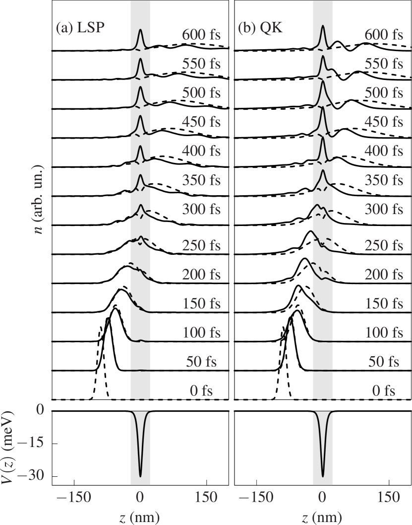
Figure 2: Evolution of the spatial charge density $n$ for a traveling wave packet impinging on the QD (see potential in the bottom panels); the solid lines show $n$ in the presence of electron-phonon scattering mechanisms as described by the (a) LSP and (b) QK approach and compared to the scattering-free evolution (dashed lines, which are identical in the two panels).

In Fig. 2 we plot the evolution of the spatial charge density [see Eq. (9)] for $z_{0}=-90$ nm, showing the LSP [panel (a)] and QK [panel (b)] results (solid lines), while the dashed lines display the free evolution (which is identical in both cases); the (same) potential profile is reported in the bottom panels, while the grey shaded background indicates the QD region as a guide to the eye. In the LSP calculations a broadening of the DC transitions of $\bar{\epsilon}=3.5$ meV has been used. The role of this value will be discussed below in Sec. III.1.3.

The free evolution allows us to distinguish three phases:

• the travel toward the QD (times $t\lesssim$ 100 fs);

• the crossing of the QD (100 fs $\lesssim t\lesssim$ 450fs);

• the moving away from the QD ($t\gtrsim$ 450fs).

Note that, even in the absence of scattering, the Gaussian shape is lost during phase (ii), however it reshapes in phase (iii). Now let us consider the case with electron-phonon interaction. Due to the capture a density peak in the QD region builds up during phase (ii) which remains there in phase (iii). In this last phase (iii), both approaches predict remarkable differences from the phonon-free case for the transmitted wave packet, in particular the appearance of spatial ripplings. The shape of the traveling continuous wave packet is thus altered by the carrier capture process, the latter happening at a well-defined position (see grey area in Fig. 2) and instant in time (phase (ii)).

While the overall behavior obtained from the two approaches is very similar, we can also recognize some differences between the respective predictions, such as, e.g., the height of the spatial rippling of the transmitted wave packet. In order to better understand the origin of these discrepancies as well as to better quantify the timescales of the carrier capture, it is convenient to look at the evolution of the bound state population. In Fig. 3 we plot $f_{1}\equiv\rho_{11}$ normalized w.r.t. the preserved total charge $\sum_{\alpha}\rho_{\alpha\alpha}=\sum_{\alpha}\rho^{0}_{\alpha\alpha}$, as predicted by the LSP and QK approaches (panel (a) and panel (b), respectively) for four different initial positions $z_{0}$ of the wave packet. Due to different numerical methods the final populations (i.e, those after the capture process is over) are slightly different, although being comparable. Both approaches predict that the wave packet initially closest (farthest) to the QD is also the first (last) one to experience the capture mechanism, an additional signature of the correct description of the local nature of carrier capture processes. The spatial shift of the initial condition essentially leads to a temporal shift of the bound state occupation.

In order to be more quantitative on the temporal window in which most of the carrier capture takes place, in Fig. 4(a) and (b) we plot once again the same result of Fig. 3 but expressing each evolution in terms of

$$\tilde{t}=t+\frac{z_{0}}{v_{k_{0}}}\,,$$ (12)

with $v_{k_{0}}=\frac{\hbar k_{0}}{m^{*}}$ being the group velocity associated with $k_{0}$. $\tilde{t}$ is thus a rescaled time such that the center of each of the four wave packets, which is roughly moving at a velocity of $v_{k_{0}}$, reaches the center of the QD at the same time $\tilde{t}=0$. In addition, in Fig. 4 we mark with a background shaded area all $\tilde{t}\in I_{\tilde{t}}$, with

$$I_{\tilde{t}}=\left[-\frac{\Delta_{t}}{2},\frac{\Delta_{t}}{2}\right]\,,$$ (13)

where the value $\Delta_{t}=\Delta_{\tilde{t}}=235$ fs will be interpreted below when discussing Fig. 5 in terms of the time-evolution of $\left.df_{1}/dt\right|_{\text{scat}}$ as provided by the LSP approach.

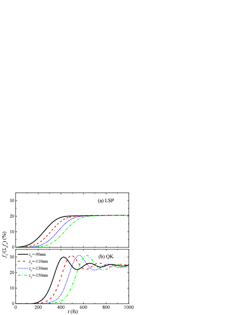
Figure 3: (Color online) Evolution of the normalized bound state population $f_{1}$ in a weakly reflecting potential when crossed by wave packets with different initial positions: $z_{0}=-90$ nm (solid black line), $z_{0}=-110$ nm (dashed red line), $z_{0}=-130$ nm (dotted blue line) and $z_{0}=-150$ nm (dashed-dotted green line); (a) evolution provided by the LSP calculations; (b) evolution obtained within the QK approach.

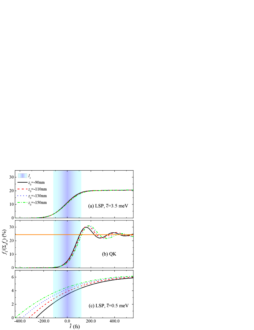
Figure 4: (Color online) Same as in Fig. 3 but expressing the evolutions in terms of the scaled time $\tilde{t}$ of Eq. (12). (a) LSP approach; (b) QK approach; (c) LSP approach with a reduced energy broadening $\bar{\epsilon}=0.5$ meV. The interval $I_{\tilde{t}}$ defined in Eq. (13) has also been added as a background shaded area, while an horizontal orange line indicates the stationary value $f_{1}\approx 24.5\%$ in the QK calculations.

Both approaches predict that most of the capture process takes place in the temporal window defined in Eq. (13). The interval $I_{\tilde{t}}$ can thus be interpreted as the temporal window in which the carrier capture takes place. Interestingly, it mostly coincides with phase (ii), which has been defined through the scattering-free evolution. Going back to the original time for the initial position $z_{0}=-90$ nm adopted in Fig. 2, in fact, this interval goes from $138.5$ fs to $391.5$ fs. However, the behavior within this interval $I_{\tilde{t}}$ is different in the two approaches.

The evolution provided by the LSP treatment is essentially symmetric around $\tilde{t}=0$, where the population is around one half of the final $f_{1}$: this time-symmetric behavior is not surprising, as the whole Markov procedure in this approach is based on a temporal symmetrization Taj et al. (2009). On the other hand, the evolutions provided by the QK treatment seem to be slightly retarded: here the population at $\tilde{t}=0$ is only around 1/5 of the final value. However, in the second half of $I_{\tilde{t}}$ the increase of $f_{1}$ predicted by QK is extremely steep. All the four lines in Fig. 4(b) in fact reach the stationary value at $\tilde{t}=\Delta_{t}/2$. In phase (ii) also the evolution predicted by the QK approach is monotonic. The retarded build-up of the bound state occupation reflects the non-Markovian nature of QK approaches, whose early-stage dynamics are governed by pseudo-probabilistic rates Rossi (2011) with energy selection rules going as $\sin(\omega t)/\omega$ Schilp et al. (1994) and, as a consequence, they are negligible in the early stages of the interaction.

In phase (iii), i.e., when the carrier capture (shaded area) is over, the QK treatment predicts a non-monotonic population evolution, while in the LSP approach the captured density essentially remains constant. The oscillations in the QK description have been interpreted as phonon-assisted Rabi oscillations inside the QD Glanemann et al. (2005). The occupation oscillates periodically between the initial electron state in the continuum and the correlated state consisting of the electron in the ground state and the emitted phonon. This behavior is similar to the case of photon-induced Rabi oscillations of atoms entering a microcavity Raimond et al. (2001). In our case, the switch on of the electron-phonon interaction is provided by the arrival of the wave packet at the QD, when phonon emission becomes possible. An abrupt switch on thus requires a strongly localized wave packet, which is only possible considering a broad range of continuum states, whose width in $k$-space is inversely proportional to the spatial size. The continuum of initial states in turn generates a continuum of Rabi frequencies with variable detuning. This leads to the rather strong damping of the oscillations seen in Figs. 3(b) and 4(b) Glanemann et al. (2005). As a consequence, these oscillations tend to vanish in few hundreds of fs after the capture process. Rabi oscillations in optically driven atomic systems are the time-domain counterpart of dressed states, i.e., mixed atom-light states which are split by the light-matter interaction. Analogously, the phonon-assisted Rabi oscillations seen here are the time-domain counterpart of polaronic states in systems with discrete states such as QDs Verzelen et al. (2002); Hameau et al. (1999) or quantum wells in strong magnetic fields Badalyan and Levinson (1988).

Another difference w.r.t. atoms moving through a microcavity is the presence of electron-phonon coupling terms which are diagonal in the electron states. These terms are also not present in the standard Jaynes-Cummings-like quantum optics models, while in strongly confined QDs the electron-phonon coupling of this type gives rise to pure dephasing Krummheuer et al. (2002). Note finally that additional simulations revealed that these oscillations tend to vanish for increasing size of the initial wave packet (typically already for widths of the order of 50 nm; not shown here). More importantly, however, the presence of these oscillations does not alter the final value of the populations of the bound states.

Such oscillations are not present in the LSP approach. As is shown analytically in appendix A, here the occupation of the bound state rises monotonically. The absence of Rabi oscillations is not surprising since, as described above, they rely on the presence of correlated electron-phonon states, which are not present in the LSP formalism working completely in the electronic subspace.

The Rabi oscillations in phase (iii) affect the spatial charge density as well, as they induce the different amplitudes of the transmitted wave-packet ripplings predicted by the two approaches in Fig. 2. The reason is an enhanced transmission probability each time the electron oscillates back to the continuum state, which thus results in an additional peak in the transmitted density seen, e.g., in Fig. 2 at $t=600$ fs.

III.1.2 Non-diagonal vs. diagonal dynamics

In previous works Reiter et al. (2007), diagonal and non-diagonal QK density matrix treatments have been compared in terms of the spatial profiles of the charge density. Here we exploit the proposed LSP treatment in order to compare diagonal vs. off-diagonal contributions to $\left.df_{1}/dt\right|_{\text{scat}}$: this will allow us to better understand the origin of the locality and the value of $\Delta_{t}$, i.e., the duration of phase (ii).

The dynamics of $f_{1}$ may be rewritten as

$$\left.\frac{df_{1}}{dt}\right|_{\text{scat}}=\left.\frac{df_{1}}{dt}\right|^{\text{diag.}}_{\text{scat}}+\left.\frac{df_{1}}{dt}\right|^{\text{off-d.}}_{\text{scat}}\quad,$$ (14)

where the first (second) term is obtained by considering only the diagonal (off-diagonal) elements of the density matrices in the r.h.s. of Eq. (20).

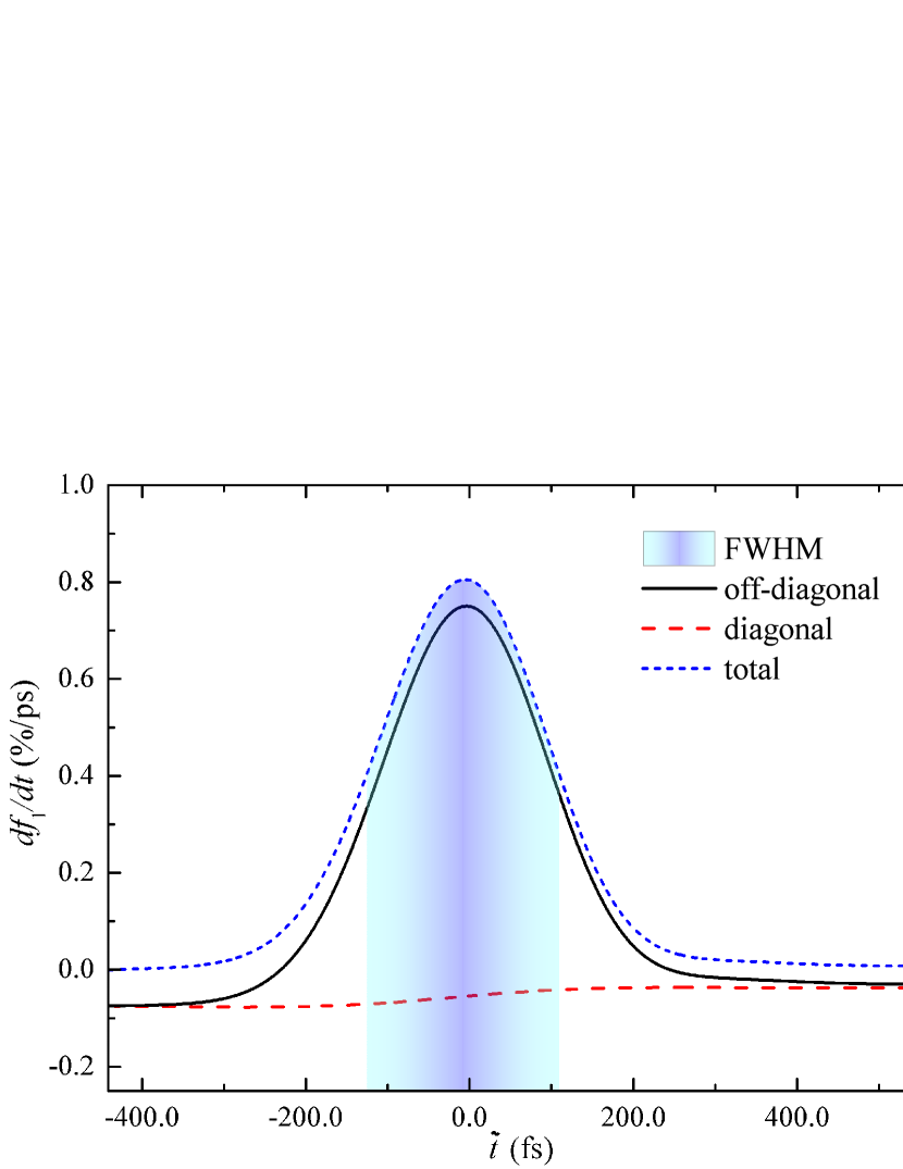
Figure 5: (Color online) Evolution of the off-diagonal (solid black line), diagonal (long dashed red curve) and total (short-dashed blue line) contributions to the scattering-induced time-derivative of $f_{1}$, for the same potential of Figs. 3 and 4 and $z_{0}=-150$ nm; in order to better show the cancelations between the two terms, the diagonal contributions are multiplied by $(-1)$. The background shaded area indicates the temporal window in which $\left.df_{1}/dt\right|_{\text{scat}}$ is bigger than half its maximum; it has a width of $\Delta_{t}=235$ fs (FWHM).

In order to understand why the diagonal contributions are not able to provide the local feature of the capture mechanisms, in Fig. 5 we plot separately the off-diagonal and diagonal contributions, multiplying the latter by $(-1)$ in order to manifest the cancelations between the two. As is evident from the long-dashed curve, the diagonal contribution to the time-derivative of $f_{1}$ is finite and positive at any instant, i.e., independent from the fact that at a given instant the wave packet is in the region of the QD or not. In contrast, the off-diagonal contributions to $\left.df_{1}/dt\right|_{\text{scat}}$ depend strongly on the position of the wave packet w.r.t. the QD: they provide negative (positive) values when the wave packet is far from (close to) the QD. The negative values, occurring when the wave packet is far from the dot, are exactly the opposite of the diagonal contributions, thus providing a net cancellation which in turn generates a vanishing derivative of the bound state population (see short-dashed line). It is thus exactly this different dependence on the wave-packet position between the diagonal and off-diagonal contributions in Eq. (14) that gives rise to the local nature of the capture processes. From a quantitative point of view the contributions from the off-diagonal elements become much bigger than the diagonal ones when the wave packet is in the region of the QD, with the former being about one order of magnitude bigger than the latter around $\tilde{t}=0$.

The steepest rise of the bound state occupation occurs when the total derivative is maximal, which essentially coincides with the time when the contribution from the off-diagonal terms is biggest. As seen in Fig. 5, this maximum almost coincides with $\tilde{t}=0$, thus inducing the essentially symmetric behavior in time already discussed after Fig. 4.

Looking at the total contribution $\left.df_{1}/dt\right|_{\text{scat}}$ we may finally be more quantitative on the duration of phase (ii), i.e., of the carrier capture process: the temporal length $\Delta_{t}$ exploited in Eq. (13) is nothing but the FWHM of the short-dashed line in Fig. 5. Note that the evaluation of the FWHM of $\left.df_{1}/dt\right|_{\text{scat}}$ is straightforward in the LSP case because it has only a single relative maximum, while additional arguments or fittings would be necessary when $f_{1}$ oscillates in time.

III.1.3 Role of the energy broadening

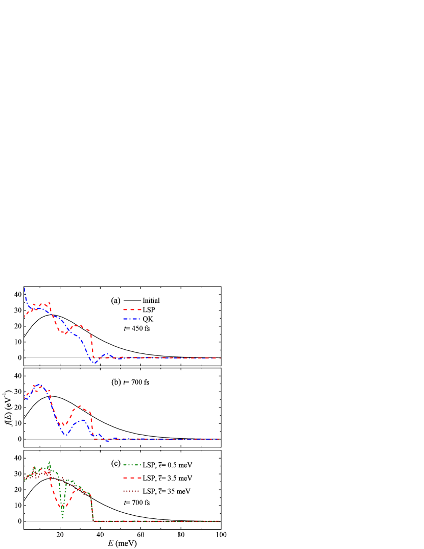
Figure 6: (Color online) Energy distribution in the continuous spectrum for the same potential of Fig. 2 with $z_{0}=-150$ nm at (a) $t=450$ fs and (b),(c) $t=700$ fs. In (a) and (b) the LSP result with the broadening parameter $\bar{\epsilon}=3.5$ meV (red dashed line) is compared to the QK result (blue dash-dotted line). In panel (c) the LSP results for three different broadenings $\bar{\epsilon}=\{0.5,3.5,35\}$ meV are plotted. The solid line in all three panels shows the initial distribution.

As has been seen in Figs. 2–5, The LSP approach well describes carrier capture except for some phenomena related to electron-phonon correlations like the phonon-assisted Rabi oscillations, which are, however, only present for very narrow wave packets. In the calculations a finite broadening of the CD transitions by $\bar{\epsilon}=3.5$ meV has been used. In this section we will now analyze the role of this broadening.

For this purpose, in Figs. 6(a) and (b) we plot the energy distribution $f(\epsilon_{\alpha})=\rho_{\alpha\alpha}/\Delta_{\epsilon_{\alpha}}$, with $\Delta_{\epsilon_{\alpha}}$ being the discretization-induced energy uncertainty around state $\alpha$, of the continuum states at two different times $t=450$ fs and $t=700$ fs obtained from the LSP calculations (dashed lines) and from the QK calculations (dash-dotted lines) for a wave packet initially located at $z_{0}=-150$ nm. The solid line shows the initial distribution. The first time, $t=450$ fs, corresponds to $\tilde{t}=8.5$ fs, i.e., essentially to the time when the maximum of the wave packet is at the QD center, the second time, $t=700$ fs, corresponds to $\tilde{t}=258.5$ fs, i.e., to a time when the wave packet has passed the QD region and the capture process is almost completed.

In the LSP calculations we see a sharp cut-off at the LO phonon energy of $36.4$ meV showing that essentially all carriers above this threshold have emitted a phonon. Furthermore, at the energy $E_{0}=\epsilon_{1}+E_{LO}=22$ meV there is a pronounced dip in the distribution caused by the missing carriers which have been captured. The width of this dip reflects the broadening of of the transitions by $\bar{\epsilon}=3.5$ meV. Also in the QK calculations the states above the LO phonon energy are essentially depopulated due to the strong scattering efficiency. However, the threshold is less pronounced, in particular at $t=450$ fs when energy-time uncertainty still plays an important role. At this time there is also no dip due to the captured electrons visible. In contrast, at $t=700$ fs the threshold behavior builds up and we observe a clear dip around $E_{0}$. While in the LSP approach the broadening has been introduced as a parameter, in the QK approach it is a result of the quantum dynamics. Here it remains at a finite value because the capture process has only a limited time window associated with the passage of the wave packet through the QD region. The broadening seen here motivated us to the use of the parameter $\bar{\epsilon}=3.5$ meV in the LSP calculations, because indeed the width of the dips in the distribution are very similar in both approaches.

As can be seen in Figs. 6(a) and (b), the QK approach displays some negativities in the electron distributions, in particular close to the threshold, which are clearly unphysical. The possibility to obtain such negativities is a consequence of the truncation of the hierarchy in the QK treatment Zimmermann and Wauer (1994); they typically vanish if the truncation is performed at a higher order of the hierarchy Krügel et al. (2006) which, however, in many systems is prohibited by the high numerical effort. Nevertheless, the magnitude of the negativities should be kept under control, as bigger values often quickly lead to strong instabilities. In the present calculations we are still far from such instabilities, as is evident from the fact that the negativities at $t=700$ fs are even less pronounced than at $t=450$ fs.

On the other hand, the symmetric structure of the LSP superoperator is able to guarantee a positive evolution also for arbitrary high interaction magnitude Rosati et al. (2014). Interestingly, the proposed approach is Lindblad already at the lowest approximation level, i.e., uncorrelated phononic and electronic subspaces, with the former taken as thermalized and the latter treated within the mean field approximation Rosati et al. (2014). Thanks to this, the LSP approach offers a versatile and extremely light alternative to QK for those situations in which the phonon dynamics or the electron-phonon correlations may be disregarded. Note that the proposed approach is computationally light both in terms of memory requirements, as it does not require the storage of the phonon-assisted density matrices (necessary on the other hand in QK) and of simulation time, which for all the results here reported is of the order of very few minutes for every simulation ran on a common desktop pc. These computational performances suggest that the LSP approach will be able to describe the carrier capture also in higher dimensional systems. Note that the original Lindblad approach has already been applied to CC transitions between fully three-dimensional states Dolcini et al. (2013).

To get more insight into the role of the broadening in the LSP calculations, in Fig. 6(c) we plot the energy distribution at $t=700$ fs for three different values of $\bar{\epsilon}=\{0.5,3.5,35\}$ meV. All other parameters are the same as in Figs.  6(a) and (b). When $\bar{\epsilon}=0.5$ meV, the broadening of the dip has a width of a few meV. For $\bar{\epsilon}=3.5$ meV the width is about 10 meV. Finally, for $\bar{\epsilon}=35$ meV the broadening is so large that the capture occurs from all states leading to a reduced distribution over the whole energy range. Obviously, the calculations with $\bar{\epsilon}=3.5$ meV exhibit the best agreement with the QK model.

In addition to the agreement with the QK calculations there is another clear argument against the use of very narrow, or in the limit delta-like, rates like in FGR for the CD transitions. This can be seen in Fig. 4(c), where we plot the occupation of the bound state as a function of time in the LSP approach for the same four initial positions $z_{0}$ as in Figs. 4(a),(b), however for the very small broadening of $\bar{\epsilon}=0.5$ meV. Interestingly, the occupation starts to grow already from the beginning, long before the wave packet has reached the QD region. A very small broadening thus also violates the locality of the capture process, much like the neglect of off-diagonal terms in the density matrix. In addition, the final value of the bound state occupation is much less than in the QK case and the LSP case with $\bar{\epsilon}=3.5$ meV. This can be understood from Fig. 6(c), which shows that the energy distribution is completely depopulated at the resonance energy for capture processes. However, because of the very small broadening there are no more electrons available to be captured in the bound state, in contrast to the case of larger broadenings when more electrons are available for the capture process.

III.2 Two bound states in a strongly reflecting potential

In this part we consider the case of a strongly reflecting potential with two bound states, namely a square well potential with depth of $-25$ meV and a width of $30$ nm, which has two bound states with energy $\epsilon_{1}=-21.4$ meV (thus we take $E_{0}=15$ meV) and $\epsilon_{2}=-11.2$ meV. The initial position of the traveling wave packet is $z_{0}=-90$ nm.

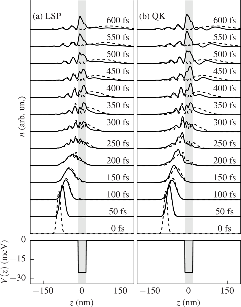
Figure 7: Evolution of the spatial charge density $n$ in the presence of a strongly reflecting square well potential (shown in the two identical bottom panels) for a traveling wave packet initially located in $z_{0}=-90$ nm as predicted by the LSP [solid lines in panel (a)] and QK approach [solid lines in panel (b)]. The scattering-free evolution (dashed lines) is identical in both panels.

In Fig. 7 we plot the evolution of the spatial electron density [see Eq. (9)], showing the LSP and QK predictions side by side; the (same) potential profile is reported in the bottom panels, while a grey background in correspondence to the QD has been added as a guide to the eye. The first important characteristic is the shape of the scattering-free distribution, i.e., the (identical) dashed lines: due to the strongly reflecting nature of the potential, the wave packet splits between a transmitted and a reflected component already in the absence of scattering mechanisms. As a consequence, a fraction of the charge does not enter into the QD region. The transmitted wave packet has a kinetic energy $\tilde{E}$ of around $20$ meV (as could be inferred from the peak position on the r.h.s. of the QD in phase (iii)), i.e., it is bigger than $E_{0}$. As will be clearer after discussing Figs. 9 and 10 below, phase (ii) is centered around a time $t_{0}\approx 275.5\text{fs}\approx|z_{0}|/v_{\tilde{E}}<|z_{0}|/v_{E_{0}}$ (see also Sec. III.1 for comparison). The reflected component is created at the end of phase (i) and survives for all the remaining evolution. Already at $t=200$ fs we may notice the presence of three peaks on the l.h.s. of the QD (centered respectively at $z=-23$ nm, $-37$ nm and $-50$ nm) moving in left direction with different velocities (at $t=600$ fs they are centered at $z=-41$ nm, $-79$ nm and $-117$ nm, respectively). Both approaches predict that the reflected charge is almost unaffected by scattering mechanisms, especially in phase (iii).

Except for its mean velocity without scattering, the behavior of the transmitted wave packet is qualitatively similar to the one of Sec. III.1: both approaches predict once again that the carrier capture induces some spatial ripplings, which are not present in a scattering-free evolution. The QK approach predicts bigger amplitudes than the LSP treatment for these oscillations, and the reason lies again in the phonon-assisted Rabi oscillations. However, from a quantitative point of view we notice that the height of the transmitted peak is particularly small. Compared to the case of Sec. III.1, this smaller transmitted peak is due to several reasons, such as more captured charge (as there are more available bound states) and less charge entering the QD (due to the reflection).

Concerning the charge within the QD, both approaches predict that it gets captured in phase (ii), i.e., when the non-reflected component of the wave packet crosses the QD (see also Figs. 9 and 10 below). In contrast to Sec. III.1, here the charge inside the QD shows an oscillating behavior in time. The timescales for these oscillations predicted by the two approaches are very similar: as an example, Fig. 7 shows that the left peak becomes the biggest one at around $500$ fs according to both predictions. The oscillations of the captured charge density are a genuine quantum mechanical effect induced by the (scattering-induced) correlations between the bound states.

To study the dynamics of the captured carriers we introduce the charge density $n_{\text{QD}}$ provided by the bound states

$$n_{\text{QD}}=\sum_{i,i^{\prime}=1}^{2}\rho_{ii^{\prime}}\psi_{i}(z)\psi^{*}_{i^{\prime}}(z)\,.$$ (15)

Except for the transient contributions of the travelling wave packet, $n_{\text{QD}}$ mostly coincides with the full charge distribution $n$ within the QD. In order to better understand the oscillatory behavior, we split this density into two parts according to

$$n_{\text{QD}}=n_{\text{f}}+n_{\text{p}}\,,$$ (16)

where

$$n_{\text{f}}=f_{1}|\psi_{1}(z)|^{2}+f_{2}|\psi_{2}(z)|^{2}$$ (17)

is the charge given by the populations of the bound states, while

$$n_{\text{p}}=2\Re[\rho_{12}\psi_{1}(z)\psi^{*}_{2}(z)]$$ (18)

($\Re$ denoting the real part) is the charge contribution given by the polarization $p=\rho_{12}$ describing the coherence between the two bound states.

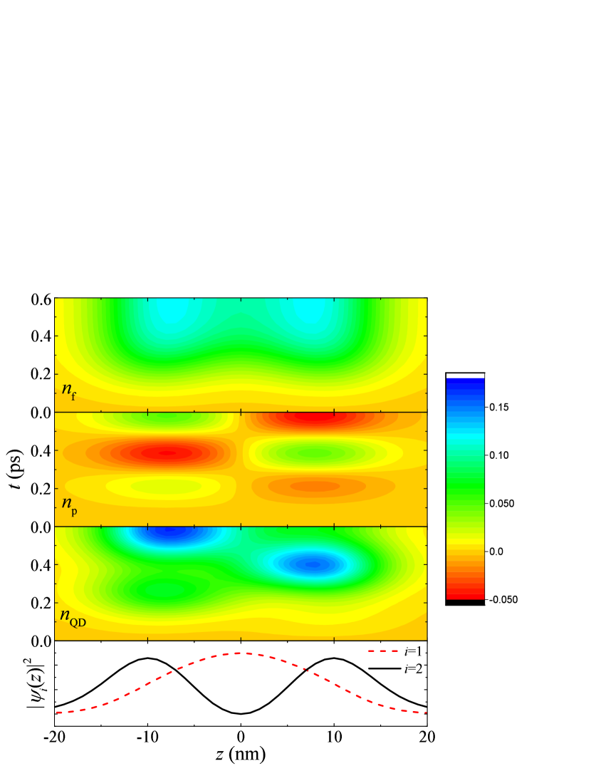
Figure 8: (Color online) Evolution of $n_{\text{f}}$ (first panel), $n_{\text{p}}$ (second panel) and of their sum $n_{\text{QD}}$ (third panel) as predicted by the LSP approach for the same case as in Fig. 7. In the fourth panel we report the spatial profile of $|\psi_{i}(z)|^{2}$ for the two bound states, $i=1,2$.

In Fig. 8 we plot $n_{\text{f}}$, $n_{\text{p}}$ and $n_{\text{QD}}$ as a function of time $t$ and position $z$ in three different panels. Concerning the diagonal contribution $n_{\text{f}}$, we see the appearance of two peaks close to the two maxima of $|\psi_{2}(z)|^{2}$: despite the fact that $|\psi_{1}(z)|^{2}$ has one only peak and that state 1 is more populated than state 2, $n_{\text{f}}$ has two peaks. Due to the even nature of both $|\psi_{1}(z)|^{2}$ and $|\psi_{2}(z)|^{2}$, the spatial distribution $n_{\text{f}}$ is completely symmetric at any time and stationary after the capture, in contrast to the electronic density $n$ within the QD region of Fig. 7. Since proportional to the product of one even and one odd bound state wavefunction, $n_{\text{p}}$ is on turn spatially anti-symmetric at any time. The temporal dependency of $n_{\text{p}}$ is all included in $\rho_{12}$, thus leading to the oscillating behaviour with frequency $(\epsilon_{2}-\epsilon_{1})/\hbar$ provided by the scattering-free evolution of $\rho$. Both $n_{\text{f}}$ and $n_{\text{p}}$ have a well defined spatial symmetry, in contrast to the electronic distribution $n$ within the QD area shown in Fig. 7. The discrepancy disappears in $n_{\text{QD}}$, where, as expected, we recognize the spatio-temporal features of $n$ for small $|z|$. At around $t$=150 fs we distinguish the appearance of a charge peak around $z\approx-8$ nm; the latter then moves to the right (following the traveling wave packet) up to around $400$ fs, where it is centered in $z\approx 8$ nm – below we will identify 150 fs and 400 fs as the edges of phase (ii), see Figs. 9 and 10. A very similar behavior is seen in the total captured charge within the QD in Fig. 7: in fact, once the transmitted wave packet leaves the QD, the spatial charge distribution in the latter is essentially given by $n_{\text{QD}}$. At times slightly bigger than $400$ fs we are at the beginning of phase (iii) (see also Figs. 9 and 10 below): the traveling wave packet leaves the QD, while $n_{\text{QD}}$ gets reflected due to the interplay between $n_{\text{f}}$ and $n_{\text{p}}$. As an example, we examine this interplay looking at what happens at $t\approx 600$ fs, when the peak of $n_{\text{QD}}$ is again within the left half of the QD. This happens because on the right half of the QD there is a strong cancelation between $n_{\text{f}}$ and $n_{\text{p}}$; in contrast, in the left half of the dot the two contributions have the same sign, thus creating a $n_{\text{QD}}$ higher than the one of $n_{\text{f}}$.

Somehow similarly to what has been seen in Sec. III.1.2, we thus conclude that the local (oscillating) behavior of the carrier capture within the QD is given by a proper interplay and cancelation between the diagonal and off-diagonal contributions (in this case to $n_{\text{QD}}$, i.e. $n_{\text{f}}$ and $n_{\text{p}}$, respectively). However, $n_{\text{p}}$ affects the spatio-temporal dynamics of the captured charge, but not its total magnitude: in fact, it is known that the spatial integral of the off-diagonal contributions to the density matrix vanishes (even in the presence of more bound states), thus not affecting the total charge brought by $n_{\text{QD}}$,

$$\int dz\,n_{\text{p}}=0\,\longrightarrow\,\int dz\,n_{\text{QD}}=\int dz\,n_{\text{f}}\,.$$ (19)

As a consequence, the inter-state correlations may shift the charge from point to point, without however modifying the net amount of total charge.

In order to catch this extremely interesting oscillating behavior, it is necessary to predict accurately not only the absolute value of $\rho_{12}$, but also its complex phase. Since both the LSP and QK approach agree in describing the oscillating evolution of the charge within the QD, it is not surprising that the two approaches predict a very similar phase of $\rho_{12}$. This is shown in Fig. 9 where, as in Sec. III.1, we add a shaded background area indicating phase (ii), which here is described through the interval $I_{t}=[t_{0}-\Delta_{t}/2,t_{0}+\Delta_{t}/2]$, where $t_{0}=275.5$ fs is the time in which $\left.df_{1}/dt\right|_{\text{scat}}$ (evaluated by the LSP approach and not plotted for the sake of shortness) is maximal, while $\Delta_{t}=276$ fs is the FWHM of $\left.df_{1}/dt\right|_{\text{scat}}$.

Figure 9: (Color online) Evolution of the real part (solid black line), imaginary part (dashed red line) and modulus (dotted blue line) of the polarization $\rho_{12}$ between the only two bound states for the same case as in Figs. 7 and 8 as predicted by the (a) LSP and (b) QK approach. The background shaded area indicates phase (ii).

In addition to the matching in terms of complex rotational phase, in Fig. 9 we observe a similar magnitude $|\rho_{12}|$, which is negligible in phase (i), increases in phase (ii) and finally stabilizes in phase (iii). Interestingly, in phase (ii) the increase of $|\rho_{12}|$ predicted by QK is monotonic, similarly to what happens for the population $f_{1}$ in Sec. III.1.

Figure 9 then shows that the period of the oscillations agrees with the Bohr period given by the energy separation between the two states Glanemann et al. (2005), i.e., $2\pi\hbar/(\epsilon_{2}-\epsilon_{1})$. Both the off-diagonal elements shown in Fig. 9 and the spatial oscillations of the captured charge shown in Figs. 7 and 8 thus demonstrate that after the capture process the carriers are in a coherent superposition of the bound states. As a consequence, neither of the two characteristics would be present in a diagonal density matrix approach.

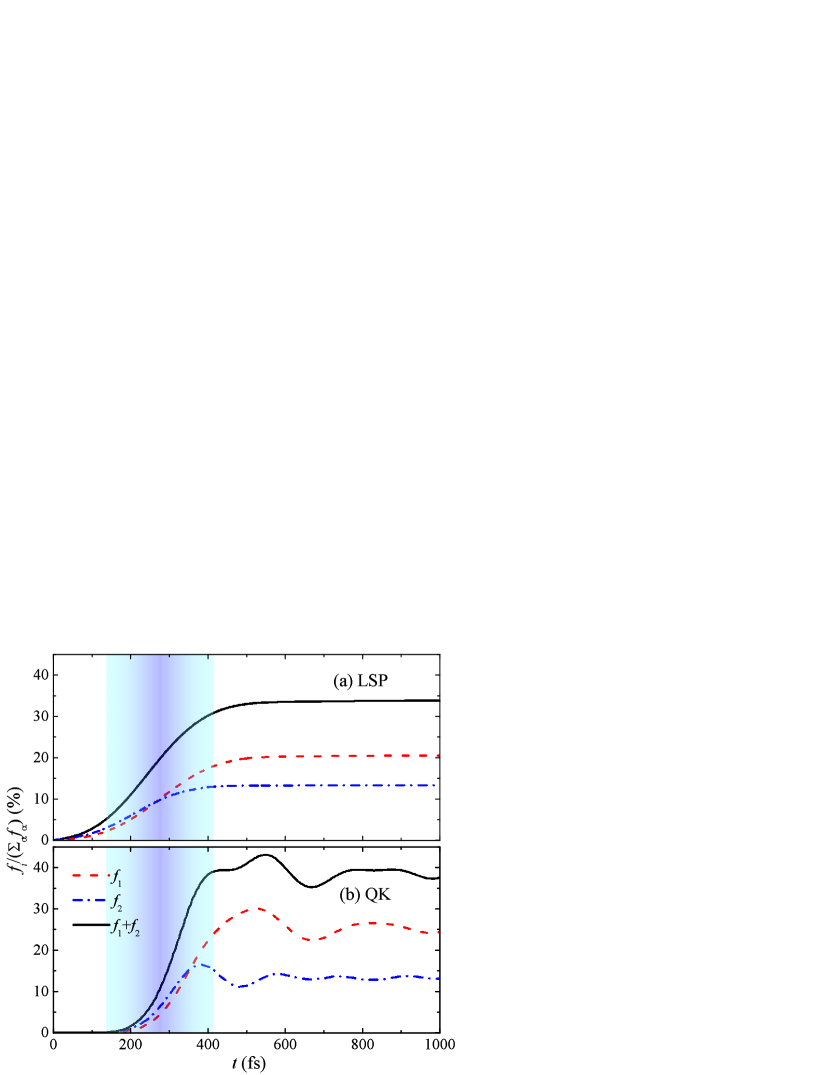
Figure 10: (Color online) Evolution of the normalized populations of the bound states $f_{1}$ (dashed red line) and $f_{2}$ (dash-dotted blue line) as well as of their sum $f_{1}+f_{2}$ (solid black line) as predicted by the (a) LSP and (b) QK approach for the same case as in Figs. 7-9. The background shaded area indicates phase (ii).

Finally, in Fig. 10 we report the evolution of the population of the bound states. Once again, the evolution of $f_{1}$ in phase (ii) (i.e., $t\in I_{t}$) predicted by QK is asymmetric w.r.t. $t_{0}$, although once again it reaches the stationary values at the end of phase (ii) and the Rabi oscillations of $f_{1}$ start only in phase (iii). Both approaches predict that the evolution of $f_{2}$ stops earlier than the end of phase (ii). This is due to the two peaks present in $|\psi_{2}(z)|^{2}$: when the wave packet reaches the second one, it has already given to state 2 most of its energetically favorable charge while crossing the first one, thus the carrier capture into state 2 is less efficient for times bigger than $t_{0}$. As in Sec. III.1, also here we find a good agreement between the LSP and QK approach.

IV Summary and conclusions

We have presented a single-particle density matrix approach which, due to its Lindblad-type nature, can describe the spatio-temporal quantum dynamics of carrier capture processes also in more complicated systems. The LSP approach is fully non-diagonal, thus able to describe the locality of the capture process, but also closed in the density matrix and positive-definite, thus stable and computationally light. The proposed approach is obtained by tailoring a recently introduced Lindblad-based equation to the specific case of carrier capture processes, in particular including the broadened energy selection rules shown by the QK studies.

By comparing the predictions provided by the LSP and QK approaches, we have identified the role played by various inter-state correlations in carrier capture processes. Most of the essential features of the spatio-temporal quantum dynamics of the carrier capture provided by the LSP and QK treatment are comparable: This is the case for the locality of the interaction (see, e.g., Fig. 4), the magnitude of the captured populations (see Figs. 3 and 10), the magnitude of inter-bound states correlations (see Fig. 9) and the spatial evolution (see Figs. 2 and 7). In particular, the very good similarity between the two predicted quantum coherences between bound states represents a clear fingerprint of the quantum nature of the approaches, which in turn has a big impact also in terms of the dynamics of the spatial charge density (see the oscillations of the captured charge in Figs. 7 and 8).

In addition to these large similarities, two differences have also been shown. The first one is a differently distributed efficiency within the interaction time window: in particular, the evolution predicted by the LSP approach is symmetric around the time in which the center of the wave packet reaches the center of the QD, a symmetry stemming from the fully time-symmetric derivation of the many-body superoperator Taj et al. (2009). The QK approach exhibits a retardation related to its non-Markovian nature. The second difference is the absence, shown also analytically, of the oscillations of the bound states population after the passage of the wave packet by the QD in the LSP treatment: these phonon-assisted Rabi oscillations, which tend to vanish in few hundreds of fs after the capture process, stem from electron-phonon correlations Glanemann et al. (2005), which are included in the QK treatment but not in the LSP approach (and more in general in most of the Markov approaches).

In summary, semiclassical treatments are the fastest ones for predicting the captured charge from homogeneous distributions, while QK approaches offer the possibility to study the spatio-temporal dynamics including also electron-phonon correlations and phonon dynamics. The proposed LSP approach offers an intermediate solution for studying the spatio-temporal quantum dynamics of the electronic wave packets also in more complicated schemes. Thanks to its stable and computationally much less-demanding nature, it is extendible to higher dimensional systems, to longer times and to phenomena involving different interaction mechanisms. In particular, strain-induced QDs Feng et al. (2012); Manzeli et al. (2015); Roldán et al. (2015); Kern et al. (2016) could give rise to interesting applications where, thanks to the possibility of a dynamical strain-engineering of the shape of the QD, they could lead to dynamical modifications of the shape of the wave packet, a key ingredient in a quantum information protocol based on the electronic charge degree of freedom.

Appendix A Lindblad approach to carrier capture

In this Appendix we explicitly write the form of the LSP superoperator and show that it always provides a monotonic rise of the bound states population. The starting point is the previously reported Rosati et al. (2014) nonlinear single-particle superoperator, which for the specific case of electron-phonon scattering and in the low-density regime, i.e. $|\rho_{\alpha\alpha^{\prime}}|\ll 1$, may be rewritten omitting the generalized Pauli factors (i.e. $(\delta_{\alpha\alpha^{\prime}}-\rho_{\alpha\alpha^{\prime}})\approx\delta_{\alpha\alpha^{\prime}}$) as

$$\left.\frac{d\rho_{\alpha\alpha^{\prime}}}{dt}\right|_{scat}\!\!\!=\frac{1}{2}\!\sum_{\bar{\alpha}\bar{\alpha}^{\prime},s}\!\!\left(\mathcal{P}^{s}_{\alpha\alpha^{\prime}\bar{\alpha}\bar{\alpha}^{\prime}}\rho_{\bar{\alpha}\bar{\alpha}^{\prime}}\!-\!\mathcal{P}^{s*}_{\bar{\alpha}\bar{\alpha}\alpha\bar{\alpha}^{\prime}}\rho_{\bar{\alpha}^{\prime}\alpha^{\prime}}\right)+\text{H.c.}\,.$$ (20)

In principle $s=(\xi,\mathbf{q},\pm)$ could label a generic scattering mechanisms, but in this paper we focus on LO phonon coupling in the $T=$0 K limit in GaAs QWRs, i.e. $s=(\text{LO},\mathbf{q},+)\equiv\mathbf{q}$. The generalized scattering rates $\mathcal{P}^{s}\equiv\mathcal{P}^{\mathbf{q}}$ may thus be written as

$$\mathcal{P}^{\mathbf{q}}_{\alpha\alpha^{\prime}\bar{\alpha}\bar{\alpha}^{\prime}}=A^{\mathbf{q}}_{\alpha\bar{\alpha}}A^{\mathbf{q}*}_{\alpha^{\prime}\bar{\alpha}^{\prime}}\,,$$ (21)

with

$$A^{\mathbf{q}}_{\alpha\bar{\alpha}}=\sqrt{\frac{2\pi}{\hbar}}g^{\mathbf{q}}_{\alpha\bar{\alpha}}\frac{e^{-\left(\frac{\epsilon_{\alpha}-\epsilon_{\bar{\alpha}}+E_{LO}}{2\bar{\epsilon}}\right)^{2}}}{(2\pi\bar{\epsilon}^{2})^{\frac{1}{4}}}\,,$$ (22)

where the energetic broadening parameter $\bar{\epsilon}$ is given by (see discussion in Sec. II)

$$\bar{\epsilon}\to\begin{cases}0\!\!&,\text{CC, }\min(\alpha,\bar{\alpha})>n_{B}\\ \bar{\epsilon}\neq 0\!\!&,\text{CD, }\max(\alpha,\bar{\alpha})>n_{B}\geq\min(\alpha,\bar{\alpha})\,,\\ \end{cases}$$ (23)

with $g^{\mathbf{q}}_{\alpha\bar{\alpha}}\equiv g^{LO\mathbf{q}+}_{\alpha\bar{\alpha}}$ and $n_{B}$ denoting the number of bound states. Note that in this work we have considered a QD with energetic separations between localized states strongly different from $E_{LO}$: as a consequence, we have disregarded all DD transitions (i.e., scattering mechanisms between bound states). In general, quasibound states may lead to polaronic contributions Magnusdottir et al. (2002); however, in this work we focus only on transitions between clearly delocalized states (e.g., energies bigger than $10$ meV) and deeply-bound states (e.g., energies smaller than $-10$ meV), which then allows us to neglect similar polaronic contributions in first approximation. The set of the Eqs. (20), (21), (22) and (23) constitutes the LSP approach that we have used.

We now also prove analytically that the LSP approach always provides monotonic evolutions of the bound state populations: for this purpose we focus on the lowest bound state $|1\rangle$, i.e. $\epsilon_{1}<\epsilon_{\alpha}$ for all $\alpha\neq 1$, and we rewrite its scattering-induced time derivative provided by Eq. (20) as

$$\left.\frac{df_{1}}{dt}\right|_{scat}=\frac{1}{2}\sum_{\bar{\alpha}\bar{\alpha}^{\prime},\mathbf{q}}\left(\mathcal{P}^{\mathbf{q}}_{11\bar{\alpha}\bar{\alpha}^{\prime}}\rho_{\bar{\alpha}\bar{\alpha}^{\prime}}-\mathcal{P}^{\mathbf{q}*}_{\bar{\alpha}\bar{\alpha}1\bar{\alpha}^{\prime}}\rho_{\bar{\alpha}^{\prime}1}\right)+\text{H.c.}\,.$$ (24)

Recalling Eqs. (22) and (21), we note that the generalized rates entering the second term in the sum of Eq. (24) are proportional to Gaussian functions in energy which provide negligible contributions: in fact,

$$\begin{split}\mathcal{P}^{\mathbf{q}*}_{\bar{\alpha}\bar{\alpha}1\bar{\alpha}^{\prime}}\propto&\,A^{\mathbf{q}}_{\bar{\alpha}\bar{\alpha}^{\prime}}g^{\mathbf{q}*}_{\bar{\alpha}1}e^{-\left(\frac{\epsilon_{\bar{\alpha}}-\epsilon_{1}+E_{LO}}{2\bar{\epsilon}}\right)^{2}}\\ \leq&\,A^{\mathbf{q}}_{\bar{\alpha}\bar{\alpha}^{\prime}}g^{\mathbf{q}*}_{\bar{\alpha}1}e^{-\left(\frac{E_{LO}}{2\bar{\epsilon}}\right)^{2}}\approx 0\,,\end{split}$$ (25)

where in the first inequality we used that $\epsilon_{1}\leq\epsilon_{\bar{\alpha}}$ by definition, while in the last approximation we used $E_{LO}\gg\bar{\epsilon}$. Inserting Eq. (25) into Eq. (24), the latter reduces to

$$\begin{split}\left.\frac{df_{1}}{dt}\right|_{scat}=&\sum_{\bar{\alpha}\bar{\alpha}^{\prime},\mathbf{q}}\mathcal{P}^{\mathbf{q}}_{11\bar{\alpha}\bar{\alpha}^{\prime}}\rho_{\bar{\alpha}\bar{\alpha}^{\prime}}\\ =&\sum_{\lambda,\mathbf{q}}\tilde{f}_{\lambda}|G^{\mathbf{q}}_{1\lambda}|^{2}\geq 0\,,\end{split}$$ (26)

where $|\lambda\rangle$ are the eigenstates of $\hat{\rho}$ with eigenvalues $\tilde{f}_{\lambda}\in\left[0,1\right]$, i.e. $\hat{\rho}|\lambda\rangle=\tilde{f}_{\lambda}|\lambda\rangle$, and $G^{\mathbf{q}}_{1\lambda}=\sum_{\bar{\alpha}}A^{\mathbf{q}}_{1\bar{\alpha}}U_{\bar{\alpha}\lambda}$, with $U_{\bar{\alpha}\lambda}=\langle\bar{\alpha}|\lambda\rangle$. Although strictly valid for the deepest bound state, the proof can easily be extended to all the bound states when the DD transitions are of minor importance, as it is the case in this work.

References

- Jacoboni and Lugli (1989) C. Jacoboni and P. Lugli, The Monte Carlo Method for Semiconductor Device Simulation (Springer, Wien, 1989).
- Rossi and Kuhn (2002) F. Rossi and T. Kuhn, “Theory of ultrafast phenomena in photoexcited semiconductors,” Rev. Mod. Phys. 74, 895–950 (2002).
- Axt and Kuhn (2004) V. M. Axt and T. Kuhn, “Femtosecond spectroscopy in semiconductors: a key to coherences, correlations and quantum kinetics,” Rep. Prog. Phys. 67, 433–512 (2004).
- Pecchia and Di Carlo (2004) A. Pecchia and A. Di Carlo, “Atomistic theory of transport in organic and inorganic nanostructures,” Rep. Prog. Phys. 67, 1497–1561 (2004).
- Haug and Koch (2004) H. Haug and S.W. Koch, Quantum Theory of the Optical and Electronic Properties of Semiconductors (World Scientific, Singapore, 2004).
- Bonitz (1998) M. Bonitz, Quantum Kinetic Theory, Teubner-Texte zur Physik (Teubner, Stuttgart, 1998).
- Datta (1997) S. Datta, Electronic Transport in Mesoscopic Systems, Cambridge Studies in Semiconductor Physics and Microelectronic Engineering (Cambridge University Press, UK, 1997).
- Makri and Makarov (1995) N. Makri and D. E. Makarov, “Tensor propagator for iterative quantum time evolution of reduced density matrices. I. Theory,” J. Chem. Phys 102, 4600 (1995).
- Vagov et al. (2011) A. Vagov, M. D. Croitoru, M. Glässl, V. M. Axt, and T. Kuhn, “Real-time path integrals for quantum dots: Quantum dissipative dynamics with superohmic environment coupling,” Phys. Rev. B 83, 094303 (2011).
- Glässl et al. (2011) M. Glässl, A. Vagov, S. Lüker, D. E. Reiter, M. D. Croitoru, P. Machnikowski, V. M. Axt, and T. Kuhn, “Long-time dynamics and stationary nonequilibrium of an optically driven strongly confined quantum dot coupled to phonons,” Phys. Rev. B 84, 195311 (2011).
- Wang et al. (2015) L. Wang, O. V. Prezhdo, and D. Beljonne, “Mixed quantum-classical dynamics for charge transport in organics,” Phys. Chem. Chem. Phys. 17, 12395–12406 (2015).
- Wang et al. (2016) L. Wang, A. Akimov, and O. V. Prezhdo, “Recent progress in surface hopping: 2011-2015,” J. Phys. Chem. Lett. 7, 2100–2112 (2016).
- Schilp et al. (1994) J. Schilp, T. Kuhn, and G. Mahler, “Electron-phonon quantum kinetics in pulse-excited semiconductors: Memory and renormalization effects,” Phys. Rev. B 50, 5435–5447 (1994).
- Fischetti (1999) M. V. Fischetti, “Master-equation approach to the study of electronic transport in small semiconductor devices,” Phys. Rev. B 59, 4901–4917 (1999).
- Knezevic (2008) I. Knezevic, “Decoherence due to contacts in ballistic nanostructures,” Phys. Rev. B 77, 125301 (2008).
- Hohenester and Pötz (1997) U. Hohenester and W. Pötz, “Density-matrix approach to nonequilibrium free-carrier screening in semiconductors,” Phys. Rev. B 56, 13177–13189 (1997).
- Bi Sun and Milburn (1999) He Bi Sun and G. J. Milburn, “Quantum open-systems approach to current noise in resonant tunneling junctions,” Phys. Rev. B 59, 10748–10756 (1999).
- Ferreira and Bastard (2015) R. Ferreira and G. Bastard, Capture and Relaxation in Self-Assembled Semiconductor Quantum Dots, (Morgan and Claypool Publishers, 2015).
- Glanemann et al. (2005) M. Glanemann, V. M. Axt, and T. Kuhn, “Transport of a wave packet through nanostructures: Quantum kinetics of carrier capture processes,” Phys. Rev. B 72, 045354 (2005).
- Reiter et al. (2006) D. Reiter, M. Glanemann, V. M. Axt, and T. Kuhn, “Controlling the capture dynamics of traveling wave packets into a quantum dot,” Phys. Rev. B 73, 125334 (2006).
- Wegscheider et al. (1997) W. Wegscheider, G. Schedelbeck, G. Abstreiter, M. Rother, and M. Bichler, “Atomically precise GaAs/AlGaAs quantum dots fabricated by twofold cleaved edge overgrowth,” Phys. Rev. Lett. 79, 1917–1920 (1997).
- Lienau et al. (2000) Ch. Lienau, V. Emiliani, T. Guenther, F. Intonti, T. Elsaesser, R. Nötzel, and K.H. Ploog, “Near field optical spectroscopy of confined excitons,” Phys. Status Solidi A 178, 471–479 (2000).
- Tatebayashi et al. (2015) J. Tatebayashi, S. Kako, J. Ho, Y. Ota, S. Iwamoto, and Y. Arakawa, “Room-temperature lasing in a single nanowire with quantum dots,” Nat. Photon. 9, 501–505 (2015).
- Heiss et al. (2013) M. Heiss, Y. Fontana, A. Gustafsson, G. Wüst, C. Magen, D. D. O’Regan, J. W. Luo, B. Ketterer, S. Conesa-Boj, A. V. Kuhlmann, J. Houel, E. Russo-Averchi, J. R. Morante, M. Cantoni, N. Marzari, J. Arbiol, A. Zunger, R. J. Warburton, and A. Fontcubert i Morral, “Self-assembled quantum dots in a nanowire system for quantum photonics,” Nat. Mater. 12, 439–444 (2013).
- Claudon et al. (2010) J. Claudon, J. Bleuse, N. S. Malik, M. Bazin, P. Jaffrennou, N. Gregersen, C. Sauvan, P. Lalanne, and J.-M. Gérard, “A highly efficient single-photon source based on a quantum dot in a photonic nanowire,” Nat. Photon. 4, 174–177 (2010).
- Loitsch et al. (2015) B. Loitsch, J. Winnerl, G. Grimaldi, J. Wierzbowski, D. Rudolph, S. Morkötter, M. Döblinger, G. Abstreiter, G. Koblmüller, and J. J. Finley, “Crystal phase quantum dots in the ultrathin core of GaAs-AlGaAs core-shell nanowires,” Nano Lett. 15, 7544–7551 (2015) .
- Bertoni et al. (2000) A. Bertoni, P. Bordone, R. Brunetti, C. Jacoboni, and S. Reggiani, “Quantum logic gates based on coherent electron transport in quantum wires,” Phys. Rev. Lett. 84, 5912 (2000).
- Ionicioiu et al. (2001) R. Ionicioiu, G. Amaratunga, and F. Udrea, “Quantum computation with ballistic electrons,” Int. J. Mod. Phys. B 15, 125–133 (2001).
- Fève et al. (2007) G. Fève, A. Mahé, J.-M. Berroir, T. Kontos, B. Plaçais, D. C. Glattli, A. Cavanna, B. Etienne, and Y. Jin, “An on-demand coherent single-electron source,” Science 316, 1169–1172 (2007).
- Feng et al. (2012) Ji Feng, Xiaofeng Qian, Cheng-Wei Huang, and Ju Li, “Strain-engineered artificial atom as a broad-spectrum solar energy funnel,” Nat. Photon. 6, 866–872 (2012).
- Manzeli et al. (2015) S. Manzeli, A. Allain, A. Ghadimi, and A. Kis, “Piezoresistivity and strain-induced band gap tuning in atomically thin MoS2,” Nano Lett. 15, 5330–5335 (2015).
- Roldán et al. (2015) R. Roldán, A. Castellanos-Gomez, E. Cappelluti, and F. Guinea, “Strain engineering in semiconducting two-dimensional crystals,” J. Phys. Condens. Matter 27, 313201 (2015).
- Kern et al. (2016) J. Kern, I. Niehues, P. Tonndorf, R. Schmidt, D. Wigger, R. Schneider, T. Stiehm, S. Michaelis de Vasconcellos, D. E. Reiter, T. Kuhn, and R. Bratschitsch, “Nanoscale positioning of single-photon emitters in atomically thin WSe2,” Adv. Mater. 28, 7101–7105 (2016).
- Rosati et al. (2015) R. Rosati, F. Dolcini, and F. Rossi, “Dispersionless propagation of electron wavepackets in single-walled carbon nanotubes,” Appl. Phys. Lett. 106, 243101 (2015).
- Rosati et al. (2015) R. Rosati, F. Dolcini, and F. Rossi, “Electron-phonon coupling in metallic carbon nanotubes: Dispersionless electron propagation despite dissipation,” Phys. Rev. B 92, 235423 (2015).
- Brum and Bastard (1986) J. A. Brum and G. Bastard, “Resonant carrier capture by semiconductor quantum wells,” Phys. Rev. B 33, 1420–1423 (1986).
- Kuhn and Mahler (1989) T. Kuhn and G. Mahler, “Carrier capture in quantum wells and its importance for ambipolar transport,” Solid-Stole Electron. 32, 1851–1855 (1989).
- Preisel and Mo/rk (1994) M. Preisel and J. Mørk, “Phonon-mediated carrier capture in quantum well lasers,” J. Appl. Phys. 76, 1691 (1994).
- Reiter et al. (2009) D. E. Reiter, E. Ya. Sherman, A. Najmaie, and J. E. Sipe, “Coherent control of electron propagation and capture in semiconductor heterostructures,” EPL 88, 67005 (2009).
- Ferreira and Bastard (1999) R. Ferreira and G. Bastard, “Phonon-assisted capture and intradot auger relaxation in quantum dots,” Appl. Phys. Lett. 74, 2818 (1999).
- Magnusdottir et al. (2003) I. Magnusdottir, S. Bischoff, A. V. Uskov, and J. Mørk, “Geometry dependence of Auger carrier capture rates into cone-shaped self-assembled quantum dots,” Phys. Rev. B 67, 205326 (2003).
- Nielsen et al. (2004) T. R. Nielsen, P. Gartner, and F. Jahnke, “Many-body theory of carrier capture and relaxation in semiconductor quantum-dot lasers,” Phys. Rev. B 69, 235314 (2004).
- Herbst et al. (2003) M. Herbst, M. Glanemann, V. M. Axt, and T. Kuhn, “Electron-phonon quantum kinetics for spatially inhomogeneous excitations,” Phys. Rev. B 67, 195305 (2003).
- Steininger et al. (1996) F. Steininger, A. Knorr, T. Stroucken, P. Thomas, and S. W. Koch, “Dynamic evolution of spatiotemporally localized electronic wave packets in semiconductor quantum wells,” Phys. Rev. Lett. 77, 550–553 (1996).
- Reiter et al. (2007) D. Reiter, M. Glanemann, V. M. Axt, and T. Kuhn, “Spatiotemporal dynamics in optically excited quantum wire-dot systems: Capture, escape, and wave-front dynamics,” Phys. Rev. B 75, 205327 (2007).
- Rosati et al. (2014) R. Rosati, R. C. Iotti, F. Dolcini, and F. Rossi, “Derivation of nonlinear single-particle equations via many-body lindblad superoperators: A density-matrix approach,” Phys. Rev. B 90, 125140 (2014).
- Taj et al. (2009) D. Taj, R. C. Iotti, and F. Rossi, “Microscopic modeling of energy relaxation and decoherence in quantum optoelectronic devices at the nanoscale,” Eur. Phys. J. B 72, 305–322 (2009).
- Rossi (2011) F. Rossi, Theory of Semiconductor Quantum Devices: Microscopic Modeling and Simulation Strategies (Springer, Berlin, 2011).
- Rosati and Rossi (2013) R. Rosati and F. Rossi, “Microscopic modeling of scattering quantum non-locality in semiconductor nanostructures,” Appl. Phys. Lett. 103, 113105 (2013).
- Rosati and Rossi (2014a) R. Rosati and F. Rossi, “Quantum diffusion due to scattering non-locality in nanoscale semiconductors,” EPL 105, 17010 (2014a).
- Rosati and Rossi (2014) R. Rosati and F. Rossi, “Scattering nonlocality in quantum charge transport: Application to semiconductor nanostructures,” Phys. Rev. B 89, 205415 (2014).
- Dolcini et al. (2013) F. Dolcini, R. C. Iotti, and F. Rossi, “Interplay between energy dissipation and reservoir-induced thermalization in nonequilibrium quantum nanodevices,” Phys. Rev. B 88, 115421 (2013).
- Glanemann et al. (2004) M. Glanemann, V. M. Axt, and T. Kuhn, “Thermal escape and capture processes in quantum wire-dot structures,” Semicond. Sci. Technol. 19, S229 (2004).
- Raimond et al. (2001) J. M. Raimond, M. Brune, and S. Haroche, “Manipulating quantum entanglement with atoms and photons in a cavity,” Rev. Mod. Phys. 73, 565–582 (2001).
- Verzelen et al. (2002) O. Verzelen, R. Ferreira, and G. Bastard, “Excitonic polarons in semiconductor quantum dots,” Phys. Rev. Lett. 88, 146803 (2002).
- Hameau et al. (1999) S. Hameau, Y. Guldner, O. Verzelen, R. Ferreira, G. Bastard, J. Zeman, A. Lemaître, and J. M. Gérard, “Strong electron-phonon coupling regime in quantum dots: Evidence for everlasting resonant polarons,” Phys. Rev. Lett. 83, 4152–4155 (1999).
- Badalyan and Levinson (1988) S. M. Badalyan and Y. B. Levinson, “Bound states of electron and optical phonon in a quantum well,” Zh. Eksp. Teor. Fiz 94, 378 (1988).
- Krummheuer et al. (2002) B. Krummheuer, V. M. Axt, and T. Kuhn, “Theory of pure dephasing and the resulting absorption line shape in semiconductor quantum dots,” Phys. Rev. B 65, 195313 (2002).
- Zimmermann and Wauer (1994) R. Zimmermann and J. Wauer, “Non-Markovian relaxation in semiconductors: An exactly soluble model,” JOL 58, 271 – 274 (1994).
- Krügel et al. (2006) A. Krügel, V. M. Axt, and T. Kuhn, “Back action of nonequilibrium phonons on the optically induced dynamics in semiconductor quantum dots,” Phys. Rev. B 73, 035302 (2006).
- Magnusdottir et al. (2002) I. Magnusdottir, A. V. Uskov, R. Ferreira, G. Bastard, J. Mørk, and B. Tromborg, “Influence of quasibound states on the carrier capture in quantum dots,” Appl. Phys. Lett. 81, 4318 (2002).