A Python program for the implementation of the $\Gamma$-method for Monte Carlo simulations

Abstract

We present a modular analysis program written in Python devoted to the estimation of autocorrelation times for Monte Carlo simulations by means of the $\Gamma$-method algorithm. We give a brief review of this method and describe the main features of the program. The latter is characterized by a user-friendly interface and an open source environment which, along with its modularity, make it a versatile tool. Finally we present a simple application as an operational test for the program.

[3][] [2][]#1#2 []unewunew []ioutilsioutils []analysisanalysis []sessionsession []plotsplots []configurationconfiguration

PROGRAM SUMMARY

Program Title: UNEW
Licensing provisions: MIT
Programming language: Python
Nature of problem: Computation of autocorrelation time for Monte Carlo generated data in an open source environment.
Solution method: Modular package implementing the $\Gamma$-method with advanced data handling.

Introduction

Monte Carlo (MC) simulations are nowadays an important and supportive tool for various theoretical and experimental research areas. A crucial aspect of MC-simulations analysis is the accurate assessment of statistical and systematic errors and the determination of the algorithm efficiency by means of the computation of the autocorrelation time. An effective way to address these issues is given by the $\Gamma$-method [6], a useful algorithm allowing a better exploitation of the generated data with respect, for example, to the usual binning techniques. The $\Gamma$-method has been first implemented in the MATLAB function UWERR .

In this work we present the UNEW project, which consists in a Python program devoted to an analysis of MC data implementing the $\Gamma$-method. The program has a modular structure that, combined with an open-source environment, allows for the possibility of extensions or embedding into preexisting software. Moreover, we provide various solutions for input data handling with a user-friendly interface.

The paper is organized as follows. In Sec. 1 we review the $\Gamma$-method, defining all the relevant estimators that the UNEW program computes. In Sec. 2 we describe the general structure of UNEW, referring to B for the details of the supporting Python modules. In Sec. 3 we present a simple application of the program to test the correct implementation of the analysis algorithm. In particular, we simulate the Ising model with two different algorithms [3, 5], analyse the generated data and compare the results with the literature [8]. Finally, we draw our comments and conclusions in Sec. 4.

1 Review of the analysis method

In this Section, we review the problem of the estimation of errors affecting MC-generated data by means of the $\Gamma$-method developed by Wolff [6]. This method relies on the evaluation the autocorrelation present in the data, allowing for an assessment of the efficiency of the MC algorithm employed.

1.1 MC simulations and preliminary concepts

Here we first sketch the main features of MC simulations, restricting our attention to the field of Statistical Mechanics. In this framework, one is interested in simulating a physical system by sequentially generating an ensemble $\{q_{i}\}_{i=1}^{N}$ of configurations, sampled according to a given distribution $P(q)$. The simulation is performed by means of an algorithm characterized by an update rule which realizes a given transition $q\rightarrow q^{\prime}$ with probability $W(q\rightarrow q^{\prime})$. We assume that the update process is a Markov chain having $P$ as its unique equilibrium distribution (see Ref. [2]), namely

$$\sum_{q\in\mathcal{S}}P(q)W(q\rightarrow q^{\prime})=P(q^{\prime}),$$

where $\mathcal{S}$ is the space of all possible configurations. Furthermore, we also require that

$$\lim_{n\to\infty}W^{(n)}(q\rightarrow q^{\prime})=P(q^{\prime}),$$ (1)

where $W^{(n)}$ denotes the probability of a transition through $n$ update steps. In the following, we consider that the ensemble $\{q_{i}\}_{i=1}^{N}$ is generated after the Markov chain has reached equilibrium. From an operative point of view, this is typically achieved by thermalizing the system for a sufficiently long time.

For each configuration $q_{i}$, one evaluates a set $\{A_{\alpha}\}_{\alpha=1}^{N_{\alpha}}$ of physical observables, called primary observables, whose MC-evaluations are denoted as $\mathcal{O}_{\alpha}(q_{i})=a^{i}_{\alpha}$, for all $i=1,\ldots,N$. The output of the simulation can then be arranged into a $N\times N_{\alpha}$ matrix. In general, one is interested in evaluating also a derived quantity, namely a function $f$ of the primary observables which we denote as

$$F=f(A_{1},A_{2},\ldots,A_{N_{\alpha}})=f(A_{\alpha}).$$

In particular, this is necessary for those observables which can not be defined configuration by configuration.

Without loss of generality, in the following we will illustrate the basic concepts of the $\Gamma$-method referring only to the analysis of primary observables. A review of the method for the case of a generic function can be found in A. We remark that the analysis method examined in this manuscript holds regardless of the algorithm used.

1.2 Review of the $\Gamma$-method

In general, data generated with MC algorithms exhibit autocorrelation: given two different time-steps of the simulation $i$ and $j$, the corresponding estimates $a_{\alpha}^{i}$ and $a_{\alpha}^{j}$ can not be considered statistically uncorrelated. The $\Gamma$-method provides an accurate assessment of the autocorrelation and thus of the error affecting correlated data.

The statistical correlation is captured by the correlation matrix, defined, under the equilibrium assumption, as

$$\Gamma_{\alpha\beta}(n) =\left\langle\left(a_{\alpha}^{i}-A_{\alpha}\right)\left(a_{\beta}^{i+n}-A_{\beta}\right)\right\rangle$$

$$=\sum_{q,q^{\prime}\in\mathcal{S}}P(q)W^{n}(q\to q^{\prime})(\mathcal{O}_{\alpha}(q)-A_{\alpha})(\mathcal{O}_{\beta}(q^{\prime})-A_{\beta}).$$

The diagonal elements $\Gamma_{\alpha}\equiv\Gamma_{\alpha\alpha}$ are called autocorrelation functions. We remark that, here and in the following, averages indicated by the bracket notation $\langle\cdot\rangle$ are taken on ensembles of identical numerical experiments with independent random numbers and initial states. Typically, the autocorrelation functions exhibit an exponential decay for large times

$$\Gamma_{\alpha}(n)\sim\exp\left(-\frac{n}{\tau}\right),\quad n\to\infty.$$ (2)

In a broad variety of cases, the decay constant $\tau$ has the same order of magnitude of the equilibration time: accordingly, as a rule of thumb, an estimate of $\tau$ can be used to verify, a posteriori, that the thermalization time of the system was much bigger than $\tau$ [6, 2].

In order to compute the statistical error and to assess the efficiency of the MC algorithm used to generate the data we define, for each observable $A_{\alpha}$, the so called integrated autocorrelation time

$$\tau_{\text{int},\alpha} =\frac{1}{2}\sum_{t=-\infty}^{\infty}\rho_{\alpha}(t)=\frac{1}{2}\frac{C_{\alpha}}{\Gamma_{\alpha}(0)},$$ (3)

where $$\rho_{\alpha}(t)$$ is the normalized autocorrelation function

$$\rho_{\alpha}(t) =\frac{\Gamma_{\alpha}(t)}{\Gamma_{\alpha}(0)}$$ (4)

and $$C_{\alpha}$$ is the autocorrelation sum given by

$$C_{\alpha} =\sum_{t=-\infty}^{\infty}\Gamma_{\alpha}(t).$$ (5)

The quantity $\tau_{\mathrm{int},\alpha}$ gives an estimate of the error of $A_{\alpha}$ due to the autocorrelation, once the Markov chain has been equilibrated. If we consider the sample mean

$$\bar{a}_{\alpha}=\frac{1}{N}\sum_{i=1}^{N}a_{\alpha}^{i},$$ (6)

as an estimator of the exact value $A_{\alpha}$, it can be shown that the resulting error $\sigma_{\alpha}$ of $\bar{a}_{\alpha}$ is given by

$$\sigma_{\alpha}^{2}\approx\frac{2\tau_{\text{int},\alpha}}{N}\Gamma_{\alpha}(0)\quad\text{for}\quad N\gg\tau.$$ (7)

Therefore the variance given by $\Gamma_{\alpha}(0)$ is modified by a factor of $\frac{2\tau_{\text{int},\alpha}}{N}$ in presence of autocorrelations.

A significant issue, that may also affect the interpretation of the analysis results, concerns the practical estimate of the integrated autocorrelation time. We first need to introduce the estimator of the autocorrelation function associated to the observable $A_{\alpha}$:

$$\bar{\Gamma}_{\alpha}(t)=\frac{1}{N-|t|}\sum_{i=1}^{N-|t|}\left(a_{\alpha}^{i}-\bar{a}_{\alpha}\right)\left(a_{\alpha}^{i+t}-\bar{a}_{\alpha}\right).$$ (8)

As a natural estimator for $\tau_{\text{int},\alpha}$ we could take

$$\bar{\tau}_{\text{int},\alpha}(N-1)=\frac{1}{2}\frac{\bar{C}_{\alpha}(N-1)}{\bar{\Gamma}_{\alpha}(0)},$$ (9)

where

$$\bar{C}_{\alpha}(N)=\bar{\Gamma}_{\alpha}(0)+2\sum_{t=1}^{N}\bar{\Gamma}_{\alpha}(t)$$ (10)

is the estimator for the autocorrelation sum (5). However, it turns out that the variance of the estimator (9) does not vanish as $N$ goes to infinity [2, 4], due to the presence of noise in the tail of $\rho(t)$. For this reason, we need to introduce a summation window $W<N$ into Eq. 9. As a side effect, such a truncation leads to a bias in the autocorrelation sum,

$$\left|\frac{\left\langle\bar{C}_{\alpha}(W)\right\rangle-C_{\alpha}}{C_{\alpha}}\right|\sim e^{-\frac{W}{\tau}},$$ (11)

which eventually translates into a systematic error associated to the error $\sigma_{\alpha}$ of the observable $A_{\alpha}$. Therefore, the choice of the summation window $W$ should be made with care: it has to be large enough compared to the decay time $\tau$ so as to reduce the systematic error, but at the same time not too large in order to avoid the inclusion of excessive noise. We take as optimal the summation window $W$ that minimizes the total relative error (sum of the statistical and systematic errors) on the considered observable [6]:

$$\frac{\delta_{\text{tot}}(\bar{\sigma}_{\alpha})}{\bar{\sigma}_{\alpha}}\approx\frac{1}{2}\min_{W}\left(e^{-\frac{W}{\tau}}+2\sqrt{W/N}\right),$$ (12)

where $\bar{\sigma}_{\alpha}^{2}=\bar{C}_{\alpha}(W)/N$. In practice, such a value of $W$ can be determined by using the automatic procedure proposed in Ref. [6]. Under the assumption of an exponential decay of the autocorrelation function, we can write

$$2\bar{\tau}_{\text{int},\alpha}(W)=\sum_{t=-\infty}^{\infty}\exp\left(-\frac{S|t|}{\bar{\tau}(W)}\right)$$ (13)

where $\bar{\tau}_{\text{int},\alpha}$ is defined in Eq. 9, $S$ is a positive factor and $\bar{\tau}(W)$ is an estimator for the decay rate $\tau$. The $S$ factor can be adjusted to account for possible discrepancies between $\tau$ and $\bar{\tau}(W)$. By inverting Eq. 13 one finds, at the first order, $\bar{\tau}(W)\sim S\bar{\tau}_{\text{int},\alpha}$: we use this value of $\bar{\tau}(W)$ to evaluate the minimum of Eq. 12, which yields the optimal value $W_{\text{opt}}$ for $W$ (see A for more details). As a consistency check of the resulting summation window, one can verify, by adjusting the value of $S$, that the plot of the integrated autocorrelation time as a function of $W$ exhibits a plateau around the optimal value.

We finally introduce a slight generalization of the framework presented above. The set of $N$ data can be divided into $R$ statistically independent replica, which in turn may be produced by parallel simulations or by splitting the data produced by a single run. Each replicum contains $N_{r}$ estimates: we denote with $a_{\alpha}^{i,r}$ the $i$-th MC estimate of the $r$-th replicum. The autocorrelation function satisfies

$$\left\langle\left(a_{\alpha}^{i,r}-A_{\alpha}\right)\left(a_{\beta}^{i+n,s}-A_{\beta}\right)\right\rangle=\delta_{rs}\Gamma_{\alpha\beta}(n).$$

Notice that $N_{r}$ must be chosen carefully, in order to effectively end up with statistically independent replica; in particular, if $N_{r}\gg\tau$ does not hold, the error estimation fails. The definition of the estimators for the general case with $R>1$ is given in A.

2 Program and library

The main purpose of the UNEW project is to provide a user-friendly interface to the implementation of the $\Gamma$-method in an open-source environment. To this end, we consider Python to be the optimal language, since it features a rich set of modules—from statistical and numerical scopes to simple yet powerful graphics capabilities—and it is also widely used in academia.

The UNEW project consists of a Python package named that can be run as a command line tool and it contains a number of Python modules serving as a supporting library. The package can be installed and used on every platform provided with an installation of Python 2.7 or higher, along with the required packages. In this section, we will briefly illustrate the structure and purpose of the modules of the package.

Input data are handled by the functions defined in the module . The $\Gamma$-method is implemented in the module , which computes both the estimators of the mean values and the associated errors in terms of the integrated autocorrelation time, as explained in Section 1. The classes defined in the module manage all the necessary resources used to plot the results of the analysis. The package provides also the module to acquire from the input parameters the necessary information to execute the analysis. The program is designed to handle an arbitrary number of files (considered as different replica of the same experiment), each one with data arranged in a $N_{k}\times N_{\alpha}$ matrix, $N_{k}$ being the number of rows of the $k$-th file. Each file can be split into further segments that will be, in turn, treated as independent replica.

At the end of the analysis process, the UNEW program returns the following output: the mean value of the selected observable(s), its error, the error of the error, the variance, the naive error computed disregarding autocorrelation, the integrated autocorrelation time along with its error, and the optimal summation window. Additionally, plots are produced for convenience of the user, showing the integrated autocorrelation time as a function of the summation window, the normalized autocorrelation, the histogram of replica and the distribution of the data.

We stress again that the program is devised so that the analysis process applies to both primary and derived observables. In B, the reader can find more details on the installation instructions and on the structure of the package.

3 Application

In this section we test our implementation of the $\Gamma$-method, illustrating an application to the well known Ising model. We consider a collection of spin variables arranged into a square lattice of size $L$ in absence of external magnetic fields, and simulate the model resorting to two different algorithms: Metropolis [3] and the single cluster Wolff algorithm [5].

The scaling of the autocorrelation time $\tau$ as a function of the correlation length $\xi$ near the phase transition (i.e. for $\xi\to\infty$) reads

$$\tau\sim\xi^{z}.$$ (14)

The dynamic critical exponent $z$ depends on the update rule employed and, as one can see from Eq. 14, it gives an assessment of the efficiency of the algorithm. The practical estimation of $z$ can be done using

$$\tau_{\text{int},\alpha}\sim L^{z_{\alpha}},\quad L\to\infty,$$

by fitting $\tau_{\text{int},\alpha}$ as a function of $L$ and extrapolating the value of $z_{\alpha}$. As a consequence, one introduces a dependence of $z$ also on the particular observable under consideration.

In our analysis, we focus on the following observables: i) the energy density $E$ and ii) the scaling quantity

$$f_{\chi}=\dfrac{L^{7/4}}{\chi},$$ (15)

where $\chi$ is the susceptibility. We will discuss our results and compare them with those given in Ref. [8] and the reader can find in B.3 a practical example of the program execution.

3.1 Results

For the test of the UNEW implementation of the $\Gamma$-method, we produced the following statistics: $10^{5}$ thermalization steps and $10^{7}$ sweeps. Our results shall be compared with those of Ref. [8]. The data have been generated with the two aforementioned algorithms at the critical temperature $T_{c}=1/\beta_{c}$, where $\beta_{c}=\frac{\ln(1+\sqrt{2})}{2}$. As an operational test to check the correct implementation of the $\Gamma$-method, we performed the analysis using also the MATLAB function UWERR , obtaining identical results.

$L$	$f_{\chi}$	$\tau_{f\chi}$	$E$	$\tau_{E}$
24	0.91723(28)	2.72(1)	0.720133(50)	3.34(1)
32	0.91649(30)	3.10(1)	0.716889(43)	3.96(2)
48	0.91613(32)	3.69(2)	0.713596(34)	4.93(2)
64	0.91574(34)	4.15(2)	0.711995(28)	5.77(3)
80	0.91605(36)	4.55(2)	0.710990(24)	6.46(3)
128	0.91633(39)	5.46(3)	0.709519(18)	8.24(5)
256	0.91555(45)	7.06(4)	0.708331(11)	11.49(8)

Table 1: Results obtained with the Wolff algorithm, performing $10^{5}$ thermalization steps and $10^{7}$ sweeps.

$L$	$f_{\chi}$	$\tau_{f\chi}$	$E$	$\tau_{E}$
24	0.91742(76)	20.4(2)	0.719938(93)	11.25(8)
32	0.91864(103)	37.5(4)	0.716591(92)	18.4(2)
48	0.91463(154)	86(1)	0.713680(92)	36.9(4)
64	0.91816(218)	165(4)	0.711867(96)	66(1)
80	0.92071(269)	248(7)	0.710837(94)	96(2)
128	0.91769(448)	696(31)	0.709485(96)	230(6)
256	0.93102(974)	2967(249)	0.708189(99)	858(42)

Table 2: Results obtained with Metropolis algorithm, performing $10^{5}$ thermalization steps and $10^{7}$ sweeps.

In Tables 2 and 1 we report the results of our analysis respectively for the single cluster and Metropolis algorithm. For each algorithm we consider different lattice sizes $L$ and evaluate $E$ and $f_{\chi}$ along with the respective autocorrelation times. Moreover, in Fig. 1 we show the UNEW plots of the autocorrelation time and of the normalized autocorrelation for the derived quantity $f_{\chi}$ in the case $L=32$.

Firstly, we notice that the simulations with the two different algorithms are in agreement at the $2\sigma$–level for the mean values of $f_{\chi}$ and $E$. Furthermore, as expected, the behaviour of the autocorrelation times (Fig. 1) exhibits a plateau starting approximately from the optimal summation window $W_{\text{opt}}$; at the same time, summing the autocorrelation function up to $W_{\text{opt}}$ allows to exclude (at least) a significant portion of its noisy tail. This has been achieved via a proper choice of the $S$ factor, as discussed in Section 1.2.

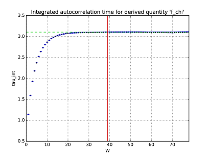
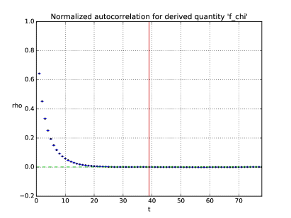
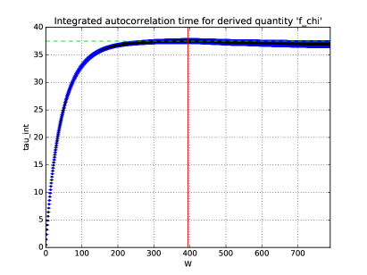
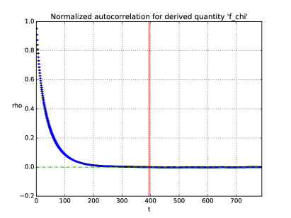
Figure 1: Integrated autocorrelation time $\tau_{f_{\chi}}$ as a function of the summation window W (left) and corresponding normalized autocorrelation $\rho$ as a function of $t$ (right) for the single cluster and Metropolis algorithms (top to bottom), with $L=32$. The red vertical line corresponds to the optimal value of the summation window.

In a typical scenario a suitable choice for $S$ is around a few units [6]: this is indeed what we find for both algorithms.

In order to assess the validity of our results, we estimate the critical dynamic exponent $z$ according to Eq. 14 and compare our findings with the existing literature. The extrapolation of $z$ for the observable $f_{\chi}$ is shown in Fig. 2 and the obtained values are reported in Table 3. In the extrapolations we exclude the data points corresponding to $L=24,32$ for the cluster algorithm, based on the improvement of the infinite volume extrapolation, that is the one of interest.

Algorithm	$z$	$\chi^{2}$
Single cluster	0.387(7)	1.64
Metropolis	2.09(1)	0.97

Table 3: Values of $z$ related to the observable $f_{\chi}$, along with their associated $\chi^{2}$, for single cluster and Metropolis algorithms.

As for the Metropolis algorithm, we recover the value $z\approx 2$ as expected for a local algorithm. Regarding the single cluster algorithm, in order to compare our results with Ref. [8], the following rescaling of $\tau$ is necessary:

$$\tau_{1C}=\tau\dfrac{m\langle C_{s}\rangle}{V},$$

where $\langle C_{s}\rangle$ is the average cluster size and $m=1$ for the two-dimensional Ising model (for further details see Ref. [5]). By doing so, the estimated value for $z$ becomes equal to $0.137(5)$, in agreement with Ref. [8].

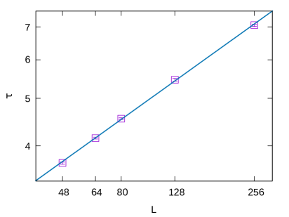
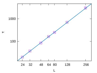
Figure 2: Log-log plots of integrated autocorrelation time of $f_{\chi}$ versus lattice size for single cluster (left) and Metropolis algorithms (right). In the former case, the data points corresponding to $L=24,32$ are excluded, resulting in an improvement of the infinite volume extrapolation.

4 Conclusions

The UNEW project provides a simple yet effective tool, in an open-source environment, to address the issue of the accurate assessment of statistical errors affecting MC-estimates of primary and derived observables. The program implements the $\Gamma$-method, which produces better estimates of the errors with respect to the usual binning techniques by taking into account the autocorrelation present in the generated data. The choice of Python as programming language aids the reuse of this software in other projects both as a standalone executable and as a library.

We showed an application of the analysis program to the Ising model in two dimensions. The simulations were performed employing the single cluster Wolff and Metropolis algorithms. Our results are identical with those obtained via UWERR and compatible with those of the existing literature, implying that the analysis method is well implemented in UNEW.

Appendix A $\Gamma$-method for derived quantities

Here we briefly illustrate how to extend the discussion of the $\Gamma$-method made in Section 1 to the more general case of a derived quantity $F=f(A_{\alpha})$ following Ref. [6]. Furthermore, we consider the case of an arbitrary number $R>1$ of replica. Accordingly, we slightly modify the notation with respect to Section 1: we define the per-replicum means as

$$\bar{a}_{\alpha}^{r}=\frac{1}{N_{r}}\sum_{i=1}^{N_{r}}a_{\alpha}^{i,r},$$ (16)

whereas $\bar{\bar{a}}_{\alpha}$ denote the estimators for the mean values of the primary observables:

$$\bar{\bar{a}}_{\alpha}=\frac{1}{N}\sum_{r=1}^{R}N_{r}\bar{a}_{\alpha}^{r}\;.$$ (17)

As an estimator of the derived quantity $f$ we take

$$\bar{\bar{F}}=f\left(\bar{\bar{a}}_{\alpha}\right).$$ (18)

We assume that the Taylor expansion of $f$ in the fluctuations is valid, allowing us to write

$$\bar{\bar{F}}\simeq F +\sum_{\alpha}f_{\alpha}\left(\bar{\bar{a}}_{\alpha}-A_{\alpha}\right)$$

$$+\frac{1}{2}\sum_{\alpha\beta}f_{\alpha\beta}\left(\bar{\bar{a}}_{\alpha}-A_{\alpha}\right)\left(\bar{\bar{a}}_{\beta}-A_{\beta}\right),$$ (19)

where we defined

$$f_{\alpha}=\frac{\partial f}{\partial A_{\alpha}},\qquad f_{\alpha\beta}=\frac{\partial^{2}f}{\partial A_{\alpha}\partial A_{\beta}},$$ (20)

evaluated at the exact values. The error $\sigma_{F}$ is related to the correlation function through

$$\sigma_{F}^{2}\simeq\frac{C_{F}}{N},$$ (21)

where the correlation sum

$$C_{F}=\sum_{\alpha\beta}f_{\alpha}f_{\beta}\sum_{t=-\infty}^{\infty}\Gamma_{\alpha\beta}(t)$$

generalizes Eq. 5. Also in this case, similarly to Eq. 7, we can rewrite

$$\sigma_{F}^{2}=\frac{2\tau_{\mathrm{int},F}}{N}v_{F},$$ (22)

thus separating the contributions coming from the effective variance of $F$

$$v_{F}=\sum_{\alpha\beta}f_{\alpha}f_{\beta}\Gamma_{\alpha\beta}(0),$$ (23)

and from the integrated autocorrelation time of $F$, given by

$$\tau_{\mathrm{int},F}=\frac{C_{F}}{2v_{F}}.$$ (24)

Exploiting the division of our data into replica, we consider as an estimator of the autocorrelation function

$$\bar{\bar{\Gamma}}_{\alpha\beta}(t)=\frac{1}{N-Rt}\sum_{r=1}^{R}\sum_{i=1}^{N_{r}-t}\left(a_{\alpha}^{i,r}-\bar{\bar{a}}_{\alpha}\right)\left(a_{\beta}^{i+t,r}-\bar{\bar{a}}_{\beta}\right),$$ (25)

which reduces to Eq. 8 for $R=1$. Nonetheless, one usually needs to compute only a few functions of the primary observables. Then, from a practical point of view instead of computing the whole correlation matrix it is more convenient to evaluate the projection

$$\bar{\bar{\Gamma}}_{F}(t)=\frac{1}{N-Rt}\sum_{r=1}^{R}\sum_{i=1}^{N_{r}-t}\,\delta_{F}^{i,r}\,\delta_{F}^{i+t,r},$$ (26)

where

$$\delta_{F}^{i,r}=\sum_{\alpha}\bar{\bar{f}}_{\alpha}\left(a_{\alpha}^{i,r}-\bar{\bar{a}}_{\alpha}\right).$$ (27)

Here the gradients $\bar{\bar{f}}_{\alpha}$ are defined as in (20), but evaluated at the mean values $\bar{\bar{a}}_{1}$, $\bar{\bar{a}}_{2},\ldots$ of the primary variables. In practice, their numerical estimates are given by the difference quotients

$$\bar{\bar{f}}_{\alpha}\approx\frac{1}{2h_{\alpha}}\big{[} f\left(\bar{\bar{a}}_{1},\bar{\bar{a}}_{2},\ldots,\bar{\bar{a}}_{\alpha}+h_{\alpha},\ldots\right)$$

$$-f\left(\bar{\bar{a}}_{1},\bar{\bar{a}}_{2},\ldots,\bar{\bar{a}}_{\alpha}-h_{\alpha},\ldots\right)\big{]},$$

with

$$h_{\alpha}=\sqrt{\frac{\bar{\bar{\Gamma}}_{\alpha\alpha}(0)}{N}}.$$

For the effective variance $v_{F}$ and the error $C_{F}$ (see Eqs. (21) and (23)) we take the following estimators:

$$\bar{\bar{v}}_{F}=\bar{\bar{\Gamma}}_{F}(0),$$ (28)

$$\bar{\bar{C}}_{F}(W)=\left[\bar{\bar{\Gamma}}_{F}(0)+2\sum_{t=1}^{W}\bar{\bar{\Gamma}}_{F}(t)\right].$$ (29)

Notice that, as already discussed for the case of the primary observables, we need to truncate the sum in Eq. 29 to a summation window $W$. We will come back to the automatic procedure to determine the optimal value of $W$ in the following.

The estimators of the error $\sigma_{F}$ in Eq. (22) and of the integrated autocorrelation time $\tau_{\mathrm{int},F}$ in Eq. (24) are simply given by

$$\bar{\bar{\sigma}}_{F}=\sqrt{\frac{\bar{\bar{C}}_{F}(W)}{N}},$$ (30)

$$\bar{\bar{\tau}}_{\mathrm{int},F}(W)=\frac{\bar{\bar{C}}_{F}(W)}{2\bar{\bar{v}}_{F}}.$$ (31)

It can be shown that the statistical error affecting $\bar{\bar{C}}_{F}(W)$ is

$$\left\langle\left(\bar{\bar{C}}_{F}(W)-C_{F}\right)^{2}\right\rangle\approx\frac{2(2W+1)}{N}C_{F}^{2}\,,\quad\text{for}\quad\tau\ll W\ll N,$$

leading to a statistical error of the error

$$\frac{\delta_{\text{stat}}\left(\bar{\bar{\sigma}}_{F}\right)}{\bar{\bar{\sigma}}_{F}}=\sqrt{\frac{W+1/2}{N}}\,.$$ (32)

For the error on the autocorrelation time, instead, if $\tau_{\text{int},F}\gg 1\gg e^{-W/\tau_{\text{int},F}}$, one gets

$$\left\langle\left(\bar{\bar{\tau}}_{\text{int},F}(W)-\tau_{\text{int},F}\right)^{2}\right\rangle\approx\frac{4}{N}\left(W+\frac{1}{2}-\tau_{\text{int},F}\right)\tau^{2}_{\text{int},F}.$$ (33)

The estimator for the derived quantity $F$ is affected by a bias due to the truncation of the power expansion (A); in order to cancel it up to the leading order $1/N$, one can exploit the division of data into replica and replace

$$\bar{\bar{F}},\bar{F}\longrightarrow\frac{R\bar{\bar{F}}-\bar{F}}{R-1},$$ (34)

where

$$\bar{F}=\frac{1}{N}\sum_{r=1}^{R}\,N_{r}f\left(\bar{a}^{r}_{\alpha}\right).$$ (35)

On the other hand, also the correlation function $\bar{\bar{\Gamma}}_{F}(t)$ is affected by a bias caused by the subtraction of the ensemble means $\bar{\bar{a}}_{\alpha}$ instead of the exact values in Eq. 25. We correct this bias at leading order by first evaluating $\bar{\bar{C}}_{F}(W)$ according to (29) and then substituting

$$\bar{\bar{\Gamma}}_{F}(t)\longrightarrow\bar{\bar{\Gamma}}_{F}(t)+\frac{\bar{\bar{C}}_{F}(W)}{N}.$$

The new resulting $\bar{\bar{\Gamma}}_{F}(t)$ is eventually taken to give a second, more refined estimate of $\bar{\bar{C}}_{F}(W)$.

Let us now come back to the windowing procedure. Solving Eq. 13 for $\bar{\tau}(W)$ yields

$$\frac{S}{\bar{\bar{\tau}}(W)}=\ln\left(\frac{2\bar{\bar{\tau}}_{\mathrm{int},F}(W)+1}{2\bar{\bar{\tau}}_{\mathrm{int},F}(W)-1}\right)=\frac{1}{\bar{\bar{\tau}}_{\mathrm{int},F}(W)}+\frac{1}{12\bar{\bar{\tau}}_{\mathrm{int},F}^{3}(W)}+\ldots,$$

which is valid for $\bar{\bar{\tau}}_{\mathrm{int}}(W)>1/2$. If $\bar{\bar{\tau}}_{\mathrm{int}}(W)\leq 1/2$, instead, we set $\bar{\bar{\tau}}(W)$ to a tiny positive value. We hence evaluate, for each integer $W$, the derivative $g(W)$ (up to a factor) of Eq. (12):

$$g(W)=\exp\left[-W/\bar{\bar{\tau}}(W)\right]-\frac{\bar{\bar{\tau}}(W)}{\sqrt{WN}}$$ (36)

and take as the optimal value $W_{\text{opt}}$ the first value of $W$ for which $g(W)$ becomes negative. If the windowing condition fails (i.e. $g(W)$ does not change sign) up to $\nu=\min_{r}N_{r}/2$, the summation window is taken as $\nu$. The correlation sum (29) is computed only up to $t=t_{\text{max}}=2\min(W_{\text{opt}},\nu)$.

Finally, we define some estimators which are useful for producing plots related to the derived quantity and to the autocorrelation time. The replica distribution

$$p_{r}=\frac{f\left(\bar{a}_{\alpha}^{r}\right)-\bar{F}}{\sigma_{F}\sqrt{N/N_{r}-1}}$$ (37)

is plotted, with a Q-value given by

$$Q=1-P\left(\frac{R-1}{2},\frac{x}{2}\right),$$ (38)

where $P$ is the regularized lower incomplete Gamma function

$$P(s,y)=\frac{1}{\Gamma(s)}\int_{0}^{y}t^{s-1}e^{-t}\;\mathrm{d}t$$

and

$$x=\sum_{r}N_{r}\,\frac{\left[f(\bar{a}_{\alpha}^{r})-\bar{F}\right]^{2}}{\bar{\bar{C}}_{F}(W_{\text{opt}})}.$$

The normalized autocorrelation function

$$\bar{\bar{\rho}}_{F}(t)=\frac{\bar{\bar{\Gamma}}_{F}(t)}{\bar{\bar{\Gamma}}_{F}(0)}$$ (39)

is also plotted along with its error (given by Eqs. (E.10) and (E.11) of Ref. [1]).

Appendix B Program description

B.1 Installation and usage

The UNEW package can be installed from source and the package tarball can be downloaded from the URL . UNEW is structured as a standard Python package that can be installed executing the following commands from a terminal prompt:

⬇

$ cd /path/to/UNEW/sources

$ pip install .

In case pip is not available, one can fall back to the script setup.py itself:

⬇

$ cd /path/to/UNEW/sources

$ python setup.py install

Alternatively, one can install the package locally for a single user with the command

⬇

$ pip install --user .

The setup script manages also the installation of the required dependencies, which are currently the Python modules numpy, scipy, matplotlib, docopt, voluptuous, PyYAML, tqdm and colorama.

Once UNEW is successfully installed on the target system, it can be run by simply calling the command unew from the command line. There are two modes of operation of the program, depending on the ways one provides the input data files to be analysed. In the first case, the user provides the input files directly on the command line; in the other one, the user specifies a directory from where the input files should be loaded. Other options can be provided to further customize the analysis. In particular, one can perform the analysis on some derived quantity of the primary observables, defined as Python functions residing in a module. For instance, suppose that a function derived is contained in a file named module.py; the user needs to let the Python interpreter know the location of the module adding it to the environment variable PYTHONPATH: in bash one can type

⬇

$ export PYTHONPATH=/path/to/module.py:$PYTHONPATH

Supposing that the input data reside in the directory data, the analysis of derived can be issued with the following command:

⬇

$ unew -d data -m module -q derived

UNEW supports also the specification of the input parameters through a configuration file written in YAML with the following general format:

⬇

!UnewConfig

directory: null or /path/to/data

replica: null or [] or [file1, file2, ...]

patterns: null or [] or [p1, p2, ...]

indices: null or [] or [1,3,4,7, ...]

ranges: null or [] or [[1,10], [20,30], ...]

R: integer (default 1)

stau: float (default 1.5)

primaries: null or [1,2,3, ...]

params: null or {par1: val1, par2: val2, ...}

module: null or module_name

functions: null or [] or [func1, func2, ...]

Such a configuration file can be generated by adding the option -C. If the file is named conf.yaml, the program can then be run with the following command:

⬇

$ unew -f conf.yaml

For further details about the usage we refer the reader to the documentation  and for a practical example we refer to B.3.

B.2 Structure of the program

In this section, we describe in a greater level of detail the modules introduced in Section 2.

The module provides the function load_files that loads the input data from a list of file paths. The returned object is a list of numpy arrays of replica. If one needs to subdivide the files into more replica or in the case there is only one file with many replica, one can pass to the function load_files the parameter R in order to split each file into $R$ replica. The total number of replica is then given by $RN_{\text{files}}$, where $N_{\text{files}}$ is the number of data files given in input. Before performing the analysis, input data are adapted through the function prepare_data into a numpy array with dimensions $(R,N_{r,\text{max}},N_{\alpha})$, where $N_{r,\text{max}}=\max_{r}N_{r}$.

The module is devoted to the implementation of the $\Gamma$-method. The classes PrimaryAnalysis and DerivedAnalysis compute the output of the program depending on whether the user chooses to analyse, respectively, primary or derived observables. In particular, the autocorrelation function is computed using the following estimators, stored as instance variables in an object of type AnalysisData:

• value, the estimator of mean values, defined in Eqs. 17 and 18;

• rep_value, an array with the values of the derived quantity taken at the per-replicum means (16);

• rep_mean, the average over replica, see Eq. (35);

• deviation, the $R\times N_{r,\text{max}}$-matrix whose entries are defined in Eq. (27).

The program then computes the errors and the autocorrelation times and stores the resulting data in the same AnalysisData object; the essential output of the program consists in the following variables:

• w_opt, the optimal value $W_{\text{opt}}$ for the summation window $W$, see Eq. (36);

• t_max, the maximum value of $t$ up to which the autocorrelation function $\bar{\bar{\Gamma}}_{F}(t)$ (26) is computed; see the discussion following Eq. 36;

• value, the unbiased expectation value of $F$ (see Eqs. (18) and (34));

• dvalue, the error of value, given by Eq. (30) with $W=W_{\text{opt}}$;

• ddvalue, the statistical error of dvalue, given by Eq. (32) with $W=W_{\text{opt}}$;

• variance, the variance of $F$, (28);

• naive_err, the error of $F$ computed disregarding autocorrelations, given by $\bar{\bar{\sigma}}_{F,\mathrm{naive}}=\sqrt{\frac{\bar{\bar{v}}_{F}}{N}}$, where $\bar{\bar{v}}_{F}$ is the variance (28);

• tau_int, the integrated autocorrelation time, given by Eq. (31) with $W=W_{\text{opt}}$;

• dtau_int, the error of tau_int, given by Eq. (33) with $W=W_{\text{opt}}$;

• tau_int_fbb, the partial autocorrelation times (31);

• dtau_int_fbb, the error of tau_int_fbb, given by Eq. (33);

• rho, the normalized autocorrelation function (39);

• drho, the error of rho, see Eqs. (E.10) and (E.11) of [1];

• qval, representing the $Q$-value for the histogram of replica distribution, given by Eq. (38).

At the end of the analysis process the program draws the plots of the integrated autocorrelation time, the autocorrelation function, the distribution of data, and the distribution of replica. The underlying graphics engine is provided by matplotlib. The plots are handled by the classes PrimaryPlot and DerivedPlot which delegate the actual drawing to the class PlotHelper: the method autoCorrTime plots the integrated autocorrelation time from $0$ to t_max, while the normalized autocorrelation function is drawn by calling normAutoCorr. Additionally, the class PlotHelper provides the method histogram to plot the replica distribution (see Eq. (37)).

Furthermore, the program validates the input parameters, whether given on the command line or through a configuration file, and reports an error to the user when it can not proceed with the analysis. The validation process relies upon the Python module voluptuous , which presents a simple interface and supports complex data structures. All the validation-related code resides in the module . This module defines a configuration class, UnewConfig, whose members provide all the essential information required to perform the analysis (e.g. data-file names, functions, specification of the observables, number of replica). The validation process is carried out by checking whether instances of this class are properly constructed. Since UNEW can be run providing the input parameters either as command line options or through a YAML configuration file, the library provides the classes CmdLineValidator and FileValidator defining the appropriate validation schema in the two cases.

B.3 Example of application

We present an example of execution of the program for the analysis of the derived observable $f_{\chi}$ as given in Eq. 15 computed with the single cluster algorithm. In general, a derived function needs to have a mandatory argument (the first one) representing the mean values (17). The user is free to customize the definition of the derived function by adding an arbitrary number of arguments, such as lattice size, critical temperature, etc. In this example the module named ising2d contains the definition of the function f_chi:

⬇

def f_chi(abb,L):

"""

Computation of f_chi = L^(7/4)/chi,

where L is the linear lattice size

and chi is the susceptibility.

abb[3] is the mean squared magnetization and

abb[4] is the mean magnetization.

"""

V = L**2

exp = 7.0/4.0

return pow(L,exp)/((abb[3]/V-(abb[4]/V)**2))

The mandatory argument is here labeled as abb. Running the program from the command line as

⬇

$ unew -d /path/to/data/directory \

-m ising2d -q f_chi -P L=32 -S 1 -R 100

one obtains the following output:

Results for derived quantity ’f_chi’:
         value: 9.164948766077298e-01
         error: 2.945798278639178e-04
error of error: 4.885053799160480e-07
   naive error: 1.183870408242084e-04
      variance: 1.401549143511278e-01
       tau_int: 3.095761227344753e+00
 tau_int error: 9.672307277108475e-03
         W_opt: 27
         t_max: 54
         Q_val: 8.919403963566213e-01

Equivalently, one can execute the program with the command line

⬇

$ unew -f config.yaml

where the file config.yaml is the configuration file:

⬇

!UnewConfig

R: 100

directory: /path/to/data/directory

functions: [f_chi]

indices: null

module: ising2d

params: {L: 32.0}

patterns: []

primaries: null

ranges: []

replica: []

stau: 1.0

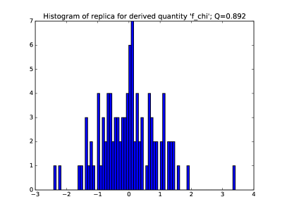
Figure 3: Distribution of replica ($R=100$) for the derived function $f_{\chi}$.

Additionally, the program produces the plots in Fig. 1 and the histogram of replica as shown in Fig. 3.

References

References

- [1] M. Luscher. Comput. Phys. Commun., 165:199–220, 2005.
- [2] N. Madras and A.D. Sokal. J. Stat. Phys., 50(1):109–186, 1988.
- [3] N. Metropolis, A.W. Rosenbluth, M.N. Rosenbluth, A.H. Teller, and E. Teller. J. Chem. Phys., 21(6):1087–1092, 1953.
- [4] M. B. Priestley. Spectral analysis and time series / M.B. Priestley. Academic Press London; New York, 1981.
- [5] U. Wolff. Phys. Rev. Lett., 62:361–364, Jan 1989.
- [6] U. Wolff. Comput. Phys. Commun., 156:143–153, 2004. Erratum-ibid. [7].
- [7] U. Wolff. Comput. Phys. Commun., 176(5):383, 2007.
- [8] Ulli Wolff. Physics Letters B, 228(3):379 – 382, 1989.