Osmotic and diffusio-osmotic flow generation at high solute concentration.
I. Mechanical approaches

Abstract

In this paper, we explore various forms of osmotic transport in the regime of high solute concentration. We consider both the osmosis across membranes and diffusio-osmosis at solid interfaces, driven by solute concentration gradients. We follow a mechanical point of view of osmotic transport, which allows us to gain much insight into the local mechanical balance underlying osmosis. We demonstrate in particular how the general expression of the osmotic pressure for mixtures, as obtained classically from the thermodynamic framework, emerges from the mechanical balance controlling non-equilibrium transport under solute gradients. Expressions for the rejection coefficient of osmosis and the diffusio-osmotic mobilities are accordingly obtained. These results generalize existing ones in the dilute solute regime to mixtures with arbitrary concentrations.

I Introduction

Osmotic transport is a subtle and non-trivial effect, that is harvested in numerous biological phenomena and applications, such as food processing in biological organisms, Sheeler and Bianchi (1987); Jensen et al. (2009) reverse osmosis for desalination, and energy generation from salinity differences, Kedem and Katchalsky (1961); Logan and Elimelech (2012); Siria et al. (2013); Werber, Osuji, and Elimelech (2016) to name a few. Traditionally, osmotic transport is described as occurring across a semi-permeable membrane, i.e., a membrane impermeable to the solute but permeable to the solvent, often water, see Fig. 1. If two reservoirs with different solute concentrations are put in contact via a semi-permeable membrane, an osmotic pressure builds up between the compartments. This pressure drop is the driving force for a flux of water from the low concentration reservoir to the highly concentrated one, until the thermodynamic equilibrium is reached. For low solute concentrations, the osmotic pressure is expressed by the van ’t Hoff law,

$$\Delta\Pi=k_{\text{B}}T\Delta c,$$ (1)

where $\Delta c$ is the difference in solute concentration between the two reservoirs. Kedem and Katchalsky (1961) The van ’t Hoff law is derived by equating the solvent chemical potential of the solvent across the membrane. Gibbs (1897); Guggenheim (1985); Klotz and Rosenberg (2008) The osmotic pressure is accordingly defined in terms of equilibrium thermodynamic properties of the system. An interesting, and quite counterintuitive, remark is that – provided it is semi-permeable – the membrane characteristics do not appear in this thermodynamic expression for the osmotic pressure.

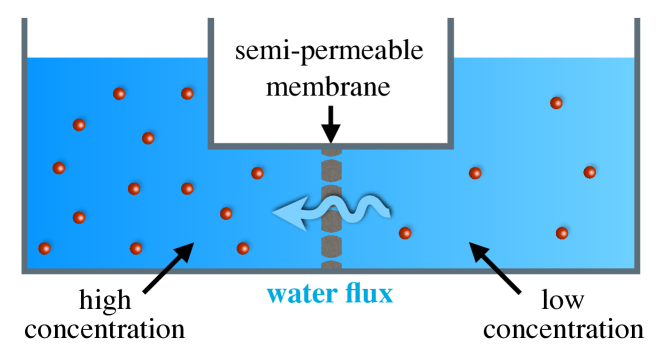
Figure 1: Geometry of osmosis. A semi-permeable membrane allows transport of water upon a solute concentration difference.

Now, when the membrane is only partially impermeable to the solute, there is still a solvent flux driven by the solute concentration imbalance. Talen and Staverman (1965a); *TS1965B; Lee et al. (2014, 2017) However the driving osmotic pressure is usually assumed to be reduced by a (dimensionless) rejection factor, say $\sigma$. Determining $\sigma$ requires to describe the detailed mass and solute transport across the membrane, and this requires to go beyond the thermodynamic description. From a general perspective, transport across a membrane is characterized within the framework of irreversible processes, via a transport matrix ${\mathbb{L}}$, relating fluxes to thermodynamic forces Kedem and Katchalsky (1961); Manning (1968); Ajdari and Bocquet (2006)

$$\left(\begin{array}[]{c}Q\\ {\color[rgb]{0,0,0}{J_{s}-cQ}}\end{array}\right)={\mathbb{L}}\times\left(\begin{array}[]{c}-\nabla p\\ -\nabla\mu\end{array}\right),$$ (2)

with $Q$ and $J_{s}$ denoting respectively the volume flux (per unit area) of the solution and of the solute through the membrane; $c$ is the solute concentration, $p$ is the pressure, and $\mu$ is the solute chemical potential. This matrix is symmetric according to Onsager’s principle. The question then amounts to characterizing the coefficients of this matrix associated with osmotic gradients. Kedem and Kachalsky rewrote these transport equations in a more explicit form as Kedem and Katchalsky (1961, 1963a); *KK1963B; *KK1963C

$$Q=-\mathcal{L}_{\text{hyd}}\left(\Delta p-\sigma k_{\text{B}}T\Delta c\right),$$ (3)

$$J_{s}=-\mathcal{L}_{\text{D}}\omega\Delta c+c(1-\sigma)Q,$$ (4)

where $\mathcal{L}_{\text{hyd}}={\color[rgb]{0,0,0}{\kappa/(\eta L)}}$ is the solvent permeance with $\kappa$ the permeability (in units of a length squared), $\eta$ the fluid viscosity, and $L$ the membrane thickness, and $\mathcal{L}_{\text{D}}=D/L$ is the solute permeability with $D$ the diffusion coefficient of the solute. The Onsager symmetry relations for Eq. (2) can be verified by exploring two limiting cases: the situation where $\Delta p=0$ yields $Q=\sigma\mathcal{L}_{\text{hyd}}c\Delta\mu$ (using $\Delta\mu=k_{\text{B}}T\Delta c/c$ in the dilute case); and the situation where $\Delta c=0$ yields $J_{s}-cQ=\sigma\mathcal{L}_{\text{hyd}}c\Delta p$, as expected. The Kedem–Kachalsky result introduces the reflection coefficient $\sigma$ mentioned previously, that is dependent in particular on the relative permeability of the membrane to the solvent and the solute. Talen and Staverman (1965a); Anderson and Malone (1974); *TS1965B Interestingly, the non-dimensional coefficients $\omega$ and $\sigma$ are expected to be linearly related, Kedem and Katchalsky (1961) as $1-\sigma\propto\omega$, a result that we will recover below. Note that the previous Kedem–Kachalsky equations are valid in the regime of dilute solute concentration, where the van ’t Hoff relationship applies. Generalizing them to mixtures with arbitrary volume fractions requires to introduce the general thermodynamic expression for the osmotic pressure and its link to non-equilibrium transport remains to be developed.

In this paper, our goal is to get some insight into the physical principles of osmosis, while exploring the high solute concentration regime. We will make use of a mechanical approach to osmosis, which is particularly illuminating to identify the force balance underlying the osmotic phenomenon. We will consider the two situations of bare osmosis across membranes and diffusio-osmosis at solid interfaces. Osmosis is expected to occur under a solute imbalance across a semi-permeable membrane, which is permeable to the solvent but not to the solute. In contrast, diffusio-osmosis is a surface-driven flow occurring under solute gradients. This form of transport has attracted increasing attention in the context of recent developments in micro- and nano-fluidic systems. Abécassis et al. (2008); Yadav et al. (2012); Lee et al. (2014); Shin et al. (2016); Shi et al. (2016); Lee et al. (2017)

To highlight the mechanical balance underlying osmotic transport, we will consider a simplified model where the effect of the membrane on the solute is described in terms of an energy barrier, see Fig. 2(a). Such an energy barrier is a crude but convenient description for the membrane, avoiding to enter into the details of the interaction of the solute with the membrane. It reduces the description to its minimal ingredients of partial or semi-permeability, and makes it amenable to explicit calculations. As we show below, it allows to explore in details how osmotic pressure builds up, even in the absence of a full semi-permeability of the membrane to the solute. We note furthermore that such barrier potential can also be physically achieved; for example, it can be generated from a nonuniform electric field acting on a polar solute in a nonpolar solvent, Debye (1954) or it can represent the nonequivalent interactions of solute and of solvent particles with a permeable membrane, e.g., charge interactions. Grim and Sollner (1957); Picallo et al. (2013) In the case of osmosis, this approach was first introduced by Manning Manning (1968) in the low concentration regime, and generalized more recently by Picallo et al. to explore the osmotic transport across perm-selective charged nanopores. Picallo et al. (2013)

On the basis of this mechanical approach, a further objective of our study is to explore osmotic phenomena in the regime of high solute concentration, where the “solute” and the “solvent” are two components of a mixture with arbitrary molar fraction. In this case, thermodynamics predicts that the thermodynamic force driving motion is a generalized osmotic pressure taking the formal expression: Barrat and Hansen (2003)

$$\Pi(c)=c{\partial f\over\partial c}-f[c]+f[c=0],$$ (5)

with $f$ the free energy density (see Appendix A for a reminder). However, how this osmotic pressure is expressed in terms of mechanical balance across a membrane (osmosis) or along an interface (diffusio-osmosis) has not been explored up to now. Our goal in the present work is accordingly to highlight how this thermodynamic expression connects to the (local) mechanical balance for osmosis and diffusio-osmosis.

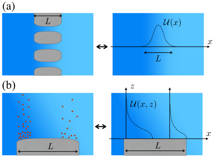
Figure 2: From the hydrodynamic picture to the mechanical approach. (a) Geometry of osmosis: from the membrane type approach to the mechanical approach describing the membrane as a potential on the solute. (b) Geometry of diffusio-osmosis: from a zoomed surface-solute interaction to a description with a potential on the solute.

II From a thermodynamic to a mechanical approach to osmosis

We consider a membrane separating two sub-volumes, containing a solvent and a solute. The concentration difference between the two volumes is $\Delta c=c_{+}-c_{-}$. As introduced above, we assume that the membrane behaves as an external potential ${\cal U}$ on the solute only, but not on the solvent molecules. It varies only along the $x$ axis. We denote $L$ the lateral range of the potential ${\cal U}$, so that ${\cal U}(-L/2)={\cal U}(L/2)=0$, and vanishes outside of this domain, see Fig. 2(a). Still we consider that the membrane is permeable to the solvent, with a permeance $\mathcal{L}_{\text{hyd}}$, relating the flux $Q$ to the pressure drop $\Delta p$ in the absence of a concentration difference: $Q=-\mathcal{L}_{\text{hyd}}\Delta p$.

We first recall results for the dilute solute regime and then extend the results to the high concentration case.

II.1 Dilute solute concentration

Before considering the general case of high solute concentration, we first revisit the case of the dilute solute concentration, as explored in Refs. 14; 26, which allows us to give the flavor of the approach. In the 1D geometry described above, the stationary solute concentration $c(x)$ obeys a Smoluchowski equation:

$$0={\partial_{t}}c= -\partial_{x}J_{s}$$

$$= -\partial_{x}\left(-D\partial_{x}c+\lambda c\,(-\partial_{x}{\cal U})+vc\right),$$ (6)

where $D$ is the diffusion coefficient and $\lambda=D/k_{\text{B}}T$ the mobility, with $k_{\mathrm{B}}$ and $T$ being the Boltzmann constant and the temperature, respectively. We further assume a low Péclet number limit, $\mathrm{Pe}=vL/D\ll 1$, such that the convective term of Eq. (6) is negligible. This is valid for low permeability (nanoporous) membranes. Since the solute current across the membrane $J_{s}$ is constant in time and spatially uniform, Eq. (6) is explicitly solved with respect to the concentration:

$$c(x)=-\Delta c\,e^{-\beta{\cal U}(x)}{\int_{x}^{L/2}dx^{\prime}\,\exp[+\beta{\cal U}(x^{\prime})]\over\int_{-L/2}^{L/2}dx^{\prime}\,\exp[+\beta{\cal U}(x^{\prime})]},$$ (7)

where $\beta=1/k_{\text{B}}T$.

Now let us focus on the force balance. It is crucial to remark that the membrane will act on the fluid as an external force, $-\partial_{x}{\cal U}$, exerted on the solute molecules. But due to action-reaction, this force acts on the fluid volume on its globality. This is for example highlighted in the force balance on the fluid, as represented by the Stokes equation along the $x$ direction:

$$0=-\partial_{x}p+c(x)(-\partial_{x}{\cal U})+\eta\nabla^{2}v,$$ (8)

where $p$ is the fluid pressure and $v$ is the flow velocity of the fluid in the $x$ direction. The driving force inducing the solvent flow is accordingly written in terms of an apparent pressure drop, $-\partial_{x}\mathcal{P}=-\partial_{x}p+c(x)(-\partial_{x}{\cal U})$. The membrane, via its potential ${\cal U}$, will therefore create an average force on the fluid, which writes per unit surface

$$-\Delta\mathcal{P}=-\Delta p+\int_{-L/2}^{L/2}dx\,c\,(-\partial_{x}{\cal U}),$$ (9)

where $\Delta$ means the difference of quantity difference between two sides. The second term of Eq. (9) can be interpreted as the osmotic contribution; one can calculate it explicitly using the concentration profile given in Eq. (7), to obtain

$$-\Delta\mathcal{P}=-\Delta p+\sigma\Delta\Pi.$$ (10)

This leads to the classical van ’t Hoff law of the osmotic pressure, $\Delta\Pi=k_{\text{B}}T\Delta c$, and the expression of the reflection coefficient $\sigma$ is obtained as

$$\sigma=1-{L\over\int_{-L/2}^{L/2}dx^{\prime}\,\exp[+\beta{\cal U}(x^{\prime})]}.$$ (11)

Equation (10) is often referred to as the Starling equation in the physiology literature, see e.g. Ref. 28.

The above result correctly recovers the case of a completely semi-permeable membrane (no solute flux across the membrane), i.e., $\beta{\cal U}\gg 1$ in this limit, and thus $\sigma\rightarrow 1$, yielding $-\Delta\mathcal{P}=-\Delta[p-\Pi]$. In the intermediate cases, although the membrane is permeable, a flow arises due to the solute concentration gradient even in the absence of a pressure gradient. When the potential is repulsive and small ${\cal U}\sim k_{\text{B}}T$, then $0<\sigma<1$; the flow is in the direction of increasing concentration. When the potential is attractive, then $\sigma<0$ and the flow reverses. Integrating Eq. (8) over the membrane area ($\mathcal{A}$) and thickness ($L$) allows us to express the total flux $Q$ as:

$$Q=-\mathcal{L}_{\text{hyd}}\left(\Delta p-\sigma k_{\text{B}}T\Delta c\right).$$ (12)

Here one may formally define the permeability $\kappa$ in terms of the averaged flow as $(1/\mathcal{A}L)\int\int dx\,d\mathcal{A}\,\nabla^{2}v\equiv-{Q}/{\kappa}$, and the corresponding permeance $\mathcal{L}_{\text{hyd}}=\kappa/(\eta L)$. These parameters, $\kappa$ and $\mathcal{L}_{\text{hyd}}$, take into account the detailed geometric specificities of the pores in the membrane. Overall Eq. (12) agrees with the Kedem–Kachalsky result in Eq. (3).

We recall that according to Ref. 3 the reflection coefficient $\sigma$ and the factor $\omega$ are linked by a linear relationship in the form $1-\sigma\propto\omega$, for diffusion through the membrane. The origin of this symmetry relationship is easily apparent from the general expression of the solute flux $J_{s}$. From the steady state condition of Eq. (6), the solute flux is expressed as

$$J_{s}=-\lambda c\,\partial_{x}\left(\mu_{\rm id}[c]+{\cal U}\right),$$ (13)

where $\mu_{\rm id}[c]=k_{\text{B}}T\ln(c/c^{*})$ is the chemical potential of the ideal (dilute) solution with solute concentration $c$, with $c^{*}$ being a reference concentration. The first term can be rewritten as $-\lambda\partial_{x}\Pi$, with $\Pi=k_{\text{B}}Tc$. The flux $J_{s}$ is spatially homogeneous ($\partial_{x}J_{s}=0$), so that one deduces

$$J_{s} =-\lambda\left(\dfrac{\Delta\Pi}{L}-{1\over L}\int_{-L/2}^{L/2}dx\,c(x)(-\partial_{x}{\cal U})\right)$$

$$=-\dfrac{\lambda}{L}\left(1-\sigma\right)\Delta\Pi,$$ (14)

and in the present case, $1-\sigma=\omega$. Note that the contribution of the total flux $Q$ to the solute flux $J_{s}$ is recovered when the convective term of Eq. (6) is accounted for. Manning (1968)

II.2 High solute concentration

We now generalize the mechanical approach to the case of a mixture with a high solute concentration. As stated earlier, the osmotic pressure is expected in this regime to deviate from its van ’t Hoff limit $\Pi=k_{\text{B}}Tc$, and is now defined in terms of the general thermodynamic expression given in Eq. (5) (as recalled in Appendix A.) Barrat and Hansen (2003)

In this regime, the solute flux $J_{s}$ entering the Smoluchowski equation for the solute now writes

$$J_{s}=-\lambda[c(x)]\,c(x)\partial_{x}\left(\mu[c(x)]+{\cal U}(x)\right),$$ (15)

where $\mu[c]$ is the chemical potential of the solute and $\lambda[c]$ the solute mobility, possibly depending on the concentration. The fluid equation of motion remains similar as above, in Eq. (8), with the membrane acting on the fluid in the form of an external force $c(x)(-\partial_{x}{\cal U})$, leading to an average force as in Eq. (9).

At equilibrium, fluxes are vanishing and the equilibrium concentration $c_{0}(x)$ thus obeys

$$\mu[c_{0}(x)]+{\cal U}(x)=\mu_{\rm res},$$ (16)

where $c_{0}(-L/2)=c_{0}(L/2)=c_{\rm res}$, such that $\mu[c_{\rm res}]=\mu_{\rm res}$. Now when there is a concentration difference $\delta c_{0}$ of the solute between the reservoirs, solvent and solute fluxes build up. In contrast to the dilute case above, one cannot solve exactly the previous equations for $c(x)$. However, one may explore the case of a small concentration difference between the reservoirs and compute the perturbation from equilibrium. This leads to a change in the concentration profile $c(x)$, which we write as $c(x)=c_{0}(x)+\delta c(x)$. At the boundaries, one has $\delta c(-L/2)=0$ and $\delta c(L/2)=\delta c_{0}$. Equivalently, this can be expressed in terms of a chemical potential difference of the solute between the reservoirs, $\Delta\mu=\mu^{\prime}[c_{\rm res}]\times\delta c_{0}$, where $\mu^{\prime}=\partial\mu/\partial c$.

To lowest order in $\delta c(x)$, the flux in Eq. (15) now writes

$$J_{s}=-\lambda[c_{0}(x)]\,c_{0}(x)\partial_{x}\left({\partial\mu\over\partial c}[c_{0}(x)]\,\delta c(x)\right).$$ (17)

Since $\partial_{x}J_{s}=0$ in the stationary state, this equation is solved with respect to $\delta c(x)$:

$$\delta c(x)=-{J_{s}\over\mu^{\prime}[c_{0}(x)]}\int_{-L/2}^{x}{dx^{\prime}\over\lambda[c_{0}(x^{\prime})]\,c_{0}(x^{\prime})}.$$ (18)

Using the boundary condition $\delta c(L/2)=\delta c_{0}$, we obtain the following expression for the flux:

$$J_{s}=-{1\over\int_{-L/2}^{L/2}{dx^{\prime}\over\lambda[c_{0}(x^{\prime})]\,c_{0}(x^{\prime})}}\Delta\mu,$$ (19)

and deduce the concentration profile $\delta c(x)$ as

$$\delta c(x)={\Delta\mu\over\mu^{\prime}[c_{0}(x)]}{{\int_{-L/2}^{x}{dx^{\prime}\over\lambda[c_{0}(x^{\prime})]\,c_{0}(x^{\prime})}}\over{\int_{-L/2}^{L/2}{dx^{\prime}\over\lambda[c_{0}(x^{\prime})]\,c_{0}(x^{\prime})}}}.$$ (20)

Using this solution for the density profile, we can now compute the corresponding driving force due to the solute acting on the fluid, according to Eq. (9):

$$\int_{-L/2}^{L/2}dx\;\delta c(x)(-\partial_{x}{\cal U}) =c_{0}(L/2)\mu^{\prime}[c_{0}(L/2)]\delta c(L/2)$$

$$-\mu^{\prime}[c_{0}(L/2)]\delta c(L/2){\int_{-L/2}^{L/2}{dx^{\prime}\over\lambda{\color[rgb]{0,0,0}{[c_{0}(x^{\prime})]}}}\over\int_{-L/2}^{L/2}{dx^{\prime}\over\lambda{\color[rgb]{0,0,0}{[c_{0}(x^{\prime})]}}\,c_{0}(x^{\prime})}},$$ (21)

where we used the equilibrium condition $\partial_{x}(\mu[c_{0}(x)]+{\cal U})=0$ to simplify the expressions.

This expression can be rewritten in terms of the thermodynamic osmotic pressure in Eq. (5), noting that

$$\Delta\Pi=\Pi(c_{\rm res}+\delta c_{0})-\Pi(c_{\rm res})=c_{\rm res}\mu^{\prime}[c_{\rm res}]\delta c_{0}.$$ (22)

The average force on the membrane in Eq. (21) can accordingly be re-expressed as

$$\int_{-L/2}^{L/2}dx\;\delta c(x)(-\partial_{x}{\cal U})=\sigma\Delta\Pi,$$ (23)

where the reflection coefficient $\sigma$ is now defined as

$$\sigma=1-{\int_{-L/2}^{L/2}{dx^{\prime}\over\lambda[c_{0}(x^{\prime})]}\over\int_{-L/2}^{L/2}{dx^{\prime}\over\lambda[c_{0}(x^{\prime})]}{c_{\rm res}\over c_{0}(x^{\prime})}}.$$ (24)

Equation (24) takes into account the non-linearities that arise from the deviation from the simple Boltzmann distribution and the dependence of mobility on concentration. The driving force is formally the same as in Eq. (10), and the solvent flux takes accordingly the form:

$$Q=-\mathcal{L}_{\text{hyd}}\left(\Delta p-\sigma\Delta\Pi\right),$$ (25)

with $\Pi$ the general thermodynamic expression in Eq. (5).

Similarly to the discussion leading to Eq. (14), we also find

$$J_{s}=-\frac{1}{\int_{-L/2}^{L/2}\frac{dx^{\prime}}{\lambda[c_{0}(x^{\prime})]}}(1-\sigma)\Delta\Pi,$$ (26)

showing that the coefficients $\sigma$ and $\omega$ are again related as $1-\sigma=\omega$.

Altogether, this derivation unifies the thermodynamic and the mechanical perspectives on the osmotic pressure.

III Diffusio-osmotic transport at high solute concentrations

We now explore similar questions for diffusio-osmotic transport. Diffusio-osmosis corresponds to the generation of solvent flow under a salinity gradient, close to a solid surface, see Fig. 3. It is an interfacially driven phenomenon, which takes its origin within the diffuse interfacial layer close to the surface where the solute interacts specifically with the surface. Ruckenstein (1981); Anderson (1989); Ajdari and Bocquet (2006) Its effects were explored in various experimental works. Siria et al. (2013); Lee et al. (2014); Shi et al. (2016); Lee et al. (2017) However only the regime of dilute solutes has been considered up to now, and we generalize the concepts to mixtures with high volume fraction of the “solute” versus the “solvent” (solute and solvent being actually two components of a mixture). This will allow us to highlight the links between diffusio-osmosis and the generalized thermodynamic osmotic pressure, as introduced in Eq. (5), and how it builds up.

The geometry is described in Fig. 3. We consider a flat surface with a solute gradient along the membrane. We denote by $x$ the coordinate parallel to the surface, and by $z$ the one orthogonal to the surface. The solute concentration gradient far from the surface is $\partial_{x}c_{\infty}$ and is assumed to be uniform along $x$. Similarly to the mechanical approach for osmosis across a membrane, we introduce an external potential ${\cal U}(z)$ from the surface, which acts only on the solute; one noticeable difference to the previous membrane case is that it now acts perpendicular to the solid surface and solute gradient (i.e. depending on $z$ but not on $x$). Typically, ${\cal U}$ is strong near the surface within a thin layer and vanishes far from the surface.

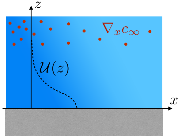
Figure 3: Geometry of diffusio-osmosis only. Far from the surface, there is a uniform gradient of solute $\nabla_{x}c_{\infty}$ parallel to the surface. The solute undergoes an external potential ${\cal U}(z)$.

We first focus on the solute distribution. We assume a thin diffusive layer, i.e., the equilibrium along $z$ is fast, so that the gradient along the surface (along $x$) is small compared with the gradient orthogonal to the surface (along $z$). In this case, local equilibrium establishes:

$$\mu[c(x,z)]+{\cal U}(z)\simeq\mu[c_{\infty}(x)].$$ (27)

In the dilute regime where $\mu[c]=k_{\text{B}}T\ln(c/c^{*})$, we find $c(x,z)=c_{\infty}(x)\exp(-{\cal U}(z)/k_{\text{B}}T)$, as discussed above. It can be more complex for high concentration $c$ of solute. In general, depending on the interaction potential ${\cal U}$, a surface excess or a surface depletion of the solute will occur at the surface.

This equation may be interpreted in terms of a mechanical balance introducing the generalized osmotic pressure. Indeed, using the local equilibrium condition Eq. (27), one gets $c(-\partial_{z}{\cal U})=c\partial_{z}\mu=c\partial_{z}\left({\partial f/\partial c}\right)\equiv\partial_{z}\Pi[c]$ (the latter two equalities being also a consequence of the Gibbs-Duhem relationship). Accordingly, one deduces that the local force (along $z$) acting on the fluid due to the wall can be interpreted in terms of the osmotic pressure as

$$c(-\partial_{z}{\cal U})=\partial_{z}\Pi[c].$$ (28)

Let us now turn to the fluid transport equation. It is described again by the Stokes equation:

$$0=-\nabla p+c(-\nabla{\cal U})+\eta\nabla^{2}\vec{v}.$$ (29)

First, the projection along the $z$ direction (with vanishing component of the velocity $v_{z}$) yields $0=-\partial_{z}p+c(-\partial_{z}{\cal U})$. Using the previous result of Eq. (28), one can rewrite this pressure balance as $\partial_{z}(p-\Pi)=0$, and obtain

$$p(x,z)-p_{\infty}=\Pi[c(x,z)]-\Pi[c_{\infty}(x)].$$ (30)

Note that here, $\Pi[c]$ indeed takes the full expression of the osmotic pressure described in Eq. (5).

This result then allows to obtain the solvent velocity profile. Indeed, injecting the pressure from Eq. (30) into the Stokes equation projected along $x$ gives

$$0=\eta\partial_{z}^{2}v_{x}-\partial_{x}(\Pi[c(x,z)]-\Pi[c_{\infty}(x)]).$$ (31)

One then obtains the velocity field in terms of the osmotic pressure:

$$v_{x}(x,z)={1\over\eta}\int_{0}^{z}\!dz^{\prime}\!\int_{z^{\prime}}^{\infty}\!dz^{\prime\prime}\partial_{x}(\Pi[c_{\infty}(x)]-\Pi[c(x,z^{\prime}\prime)]).$$ (32)

Here the no slip boundary condition at the surface and a vanishing velocity gradient at infinity have been assumed.

This expression can be rearranged using again the Gibbs-Duhem relation, $d\Pi=cd\mu$ (see Eq. (5)), leading to

$$v_{x}(x,z)={1\over\eta}\!\int_{0}^{z}\!\!\!dz^{\prime}\!\int_{z^{\prime}}^{\infty}\!\!\!dz^{\prime\prime}\left(c_{\infty}(x)-c(x,z^{\prime\prime})\right)\partial_{x}\mu[c_{\infty}(x)].$$ (33)

Note that we used $\partial_{x}\mu[c(x,z)]=\partial_{x}\mu[c_{\infty}(x)]$ resulting from the local equilibrium in Eq. (27). Finally, using $c_{\infty}(x)\partial_{x}\mu[c_{\infty}(x)]=\partial_{x}\Pi[c_{\infty}(x)]$ in the bulk, one obtains a more transparent expression for the diffusio-osmotic velocity far from the surface as

$$v_{\infty}=K_{DO}\partial_{x}\Pi[c_{\infty}(x)],$$ (34)

with the diffusio-osmotic mobility $K_{DO}$ given as

$$K_{DO}=-\frac{1}{\eta}\int_{0}^{\infty}dz^{\prime}\,z^{\prime}\,\left({c(x,z^{\prime})\over c_{\infty}(x)}-1\right).$$ (35)

Note that $\eta$ can also be assumed to depend on the concentration $c$. In this case, ${1/\eta}$ in $K_{DO}$ has to be integrated along $z$ as well. The effect of hydrodynamic slippage on the surface can also be taken into account, along the same lines as in Ref. 15, leading to an enhancement factor $(1+b/L_{s})$, where $b$ is the slip length and $L_{s}$ is the typical width of the diffuse interface. The results for diffusio-osmosis in Eqs. (34) and (35) are analogous to electro-osmosis and other surface-driven flows, with the mobility defined in terms of the first spatial moment of a density profile (solute concentration profile for diffusio-osmosis and charge density profile in the case of electro-osmosis).

To sum up, a solute gradient generates an interfacial flow of the fluid. As highlighted in Eq. (34), this flow takes its origin in an osmotic pressure gradient occurring within the diffuse layer close to the surface. Quantitatively, this flow is quantified by the value of the diffusio-osmotic mobility $K_{DO}$, which is non-zero only if there is surface excess or surface depletion of the solute. As a rule of thumb, its sign will be dominantly determined by the adsorption $\Gamma=\int_{0}^{\infty}dz^{\prime}\,\left({c(x,z^{\prime})/c_{\infty}(x)}-1\right)$. If there is a surface excess ($\Gamma>0$), the flow of water goes towards the low concentrated area ($K_{DO}<0$). Respectively, if there is a surface depletion, the flow of water reverses. But in case of a complex concentration profile, for instance with an oscillatory spatial dependence on $z$ due to layering, the sign of $K_{DO}$ may be expected to differ from the adsorption $\Gamma$. In this case, no obvious conclusion can be made for the direction of the diffusio-osmotic velocity and a full calculation has to be made.

The general expression for the diffusio-osmotic velocity, in Eqs. (34) and (35), are very similar to the corresponding expression for the dilute solution, Ruckenstein (1981); Anderson (1989); Ajdari and Bocquet (2006) but the result in Eq. (34) makes it very clear that the diffusio-osmotic flux is indeed driven by the thermodynamic osmotic pressure gradient $\partial_{x}\Pi[c_{\infty}(x)]$.

IV Discussion and conclusions

We conclude with a few words on possible extensions and implications of the results derived here.

IV.1 Coupling osmosis and diffusio-osmosis

First, while the previous derivations considered osmosis and diffusio-osmosis separately, one may consider a coupled situation in which both phenomena act jointly. Let us consider accordingly a general situation of a partially permeable membrane, similar to Fig. 2(b), now with a membrane interface interacting with solute particles. In full generality, the two transport phenomena are intimately coupled in the force balance and the situation is complex to disentangle. However some conclusions can be drawn in the limit where the pore size is large as compared to the interaction range of the surface potential, i.e. small diffuse layer. In this case, one may decompose the interaction potential into two contributions : ${\cal U}(x,z)={\cal U}_{\infty}(x)+{\color[rgb]{0,0,0}{{\cal U}_{0}(x,z)}}$, where ${\cal U}_{0}(x,z)$ is the surface interaction inside the membrane, which vanishes beyond the diffuse layer close to the surfaces; and ${\cal U}_{\infty}(x)$ is independent of $z$ and describes a global energy barrier associated with the membrane, see Fig.4. Under this assumption, this situation is amenable to a full calculation, which we report in Appendix B. As shown, the flow across the membrane still obeys a general Kedem–Kachalsky formula as in Eq. (25), with $\Pi$ the general osmotic force, but with a reflection coefficient which now contains the coupled effects of osmosis and diffusio-osmosis:

$$\sigma=\sigma_{O}+\sigma_{DO}{\color[rgb]{0,0,0}{-\sigma_{O}\sigma_{DO}}},$$ (36)

where $\sigma_{O}$ is the osmotic reflection coefficient given by Eq. (24) and the diffusio-osmotic reflection coefficient is defined as $\sigma_{DO}={\eta K_{DO}}/{\kappa}$, where $K_{DO}$ given in Eq. (35) is the diffusio-osmotic reflection coefficient, and $\kappa$ the permeability.

The last term in Eq. (36) accounts for a negative feedback coupling between osmosis and diffusio-osmosis. Although obtained in the limit of small diffuse layer, it exhibits a proper symmetry, as can be verified by considering various limiting situations. If the membrane is completely semi-permeable with $\sigma_{O}=1$, then no solute flux occurs through the membrane and the diffusio-osmotic contribution in $\sigma_{DO}(1-\sigma_{O})$ vanishes. Reversely one also obtains $\sigma=1$ when $\sigma_{DO}=1$. A second note is that this coupled contribution hints to numerous possibilities to tune the flux through the membrane. With a given $\sigma_{O}<1$, it is possible to enhance (respectively, diminish) $\sigma$ – and thus the flux through the membrane – with a slight surface depletion (respectively, excess) on the surface. How this result may be generalized to any geometry remains to be explored.

IV.2 Outlook

In summary, we have explored various forms of osmotic transport in the regime of high solute concentration. Both osmosis across model membranes and diffusio-osmosis at the interface with solid substrates were considered. We have specifically focused our approach on the mechanical balance leading to solvent flow under solute concentration gradients and explored the regime of high solute concentration. We demonstrate in particular how the general expression of the osmotic pressure for mixtures, as obtained classically from the thermodynamic framework, emerges from the mechanical balance controlling non-equilibrium transport under solute gradients. The van ’t Hoff expression for the osmotic pressure, $\Pi=k_{\text{B}}Tc$, is accordingly replaced by its general thermodynamic counterpart, $\Pi=c\,\partial_{c}f-f[c]+f[c=0]$ (with $f$ the free energy density), which is valid for arbitrary composition of the “solvent”/“solute” mixture. This generalizes the existing results obtained in the dilute solute regime. In the second paper in this series, we will provide a numerical validation of the present results by means of molecular dynamic simulations. Yoshida, Marbach, and Bocquet (2017)

An interesting consequence of the result in Eq. (34) is that a non-linear “sensing” may originate from non-linearities of the osmotic pressure versus the solute concentration. This may occur, e.g., for dense colloidal or polymer suspensions, as well as from a concentration dependent mobility $K_{DO}$ (e.g., in ionic cases where $K_{DO}$ scales as the square of the concentration dependent Debye length). Finally let us discuss again the ingredients required to describe our osmotic membrane. In the case of osmosis, we considered a model membrane, where the details of the membrane are reduced to its minimal ingredients and modeled as an external potential acting on the solute. As shown above, this simplified picture is extremely fruitful to gain insight into the mechanical balance at play. But it also points to the fact that osmosis does not require per se a solid membrane to be expressed. One may consider experimental situations where such a potential is built on the basis of optical or electrical forces, using e.g. optical tweezers to repel “solute” particles, or dielectro-phoretic potential traps. Such “osmosis without a membrane” configuration would be highly interesting to develop, as it would simplify many aspects of clogging and pore blocking which occur for standard porous membranes. However designing such non-solid wells for molecular solutes, such as salts, remains a considerable challenge.

Appendix

Appendix A : General expression of the osmotic pressure

We recall below the general expression of the osmotic pressure given in Eq. (5). The derivation is directly inspired by the presentation in Ref. 27.

Consider two compartments separated by a perfectly semi-permeable membrane. We consider on one side solvent with density $\rho_{A}$ and solute with density $\rho_{B}$. On the other side there are solvent with density $\rho^{\prime}_{A}$ and solute with density $\rho^{\prime}_{B}$. It is convenient to write the Helmholtz free energy of the mixture:

$$F(T,V,N_{A},N_{B})=-pV+\mu_{A}N_{A}+\mu_{B}N_{B},$$ (37)

where $V$ is the system volume, $N_{A}$ and $N_{B}$ are the number of solvent and solute particles, respectively. We used Euler’s theorem with $F=U-TS$, with $U$ the internal energy and $S$ the entropy.

The osmotic pressure is the difference in pressure between both sides:

$$\Pi=P-P^{\prime}= \mu_{A}(\rho_{A}-\rho^{\prime}_{A})+\mu_{B}\rho_{B}-\mu^{\prime}_{B}\rho^{\prime}_{B}$$

$$+f(T,\rho_{A}^{\prime},\rho_{B}^{\prime})-f(T,\rho_{A},\rho_{B}),$$ (38)

where $f=F/V$ is now the free energy density. We also used the fact that the chemical potentials of the solvent at equilibrium are equal on both sides of the membrane:

$$\mu_{A}=\frac{\partial f(T,\rho_{A}^{\prime},\rho_{B}^{\prime})}{\rho_{A}^{\prime}}=\frac{\partial f(T,\rho_{A},\rho_{B})}{\rho_{A}}.$$ (39)

Now we define $\rho=\rho_{A}+\rho_{B}$ and $c=\rho_{B}$ in each compartment. As a result, (considering constant $\rho$,) we have in this new space variable

$$\mu_{A}=\frac{\partial f}{\partial c}\frac{\partial c}{\partial\rho_{A}}=0\hskip 5.69054pt{\rm and}\hskip 5.69054pt\mu_{B}=\frac{\partial f}{\partial c}\frac{\partial c}{\partial\rho_{B}}=\frac{\partial f}{\partial c}.$$ (40)

We can thus express the osmotic pressure directly as

$$\Pi=\frac{\partial f}{\partial c}c-\frac{\partial f}{\partial c^{\prime}}c^{\prime}+f(c^{\prime})-f(c),$$ (41)

which is exactly Eq. (5), with $c^{\prime}=0$. In the low density regime, we recall that $f(c)=ck_{\text{B}}T\ln c+(1-c)k_{\text{B}}T\ln(1-c)$ and thus we recover the limit of dilute systems, in which $\Pi=k_{\text{B}}T(c-c^{\prime})$.

Appendix B : Coupled osmotic and diffusio-osmotic flows

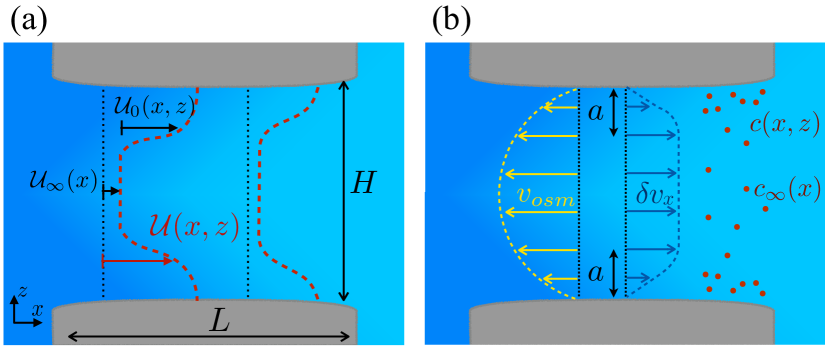
Figure 4: Geometry of a membrane pore, in which combined osmotic and diffusio-osmotic transport across the membrane take place. (a) Interaction potential expressed as ${\cal U}(x,z)={\cal U}_{\infty}(x)+{\cal U}_{0}(x,z)$, where ${\cal U}_{0}(x,z)$ vanishes outside the diffuse layers. (b) Illustration of the decomposed velocity profiles $v_{x}=v_{osm}+\delta v_{x}$ within the pore. The typical thickness of the diffuse layer is denoted by $a$, and the typical size of the pore by $H$.

Here we examine the case of a membrane with pores of a finite size interacting with the solute. Typically, the geometry under consideration is that of Fig. 4. To simplify calculations, we assume a slit geometry with a planar pore of length $L$ and width $H$ (and invariant by translation in the perpendicular direction). We make also a further hypothesis and assume here that the interaction potential of the membrane with the solute can be decomposed as

$${\cal U}(x,z)={\cal U}_{\infty}(x)+{{\cal U}_{0}(x,z)},$$ (42)

where ${\cal U}(x,z)$ is non zero only between $-L/2$ and $L/2$, ${\cal U}_{\infty}(x)$ describes the global energy barrier associated with the membrane, and ${\cal U}_{0}(x,z)$ describes the specific interaction with the membrane pore surface, and vanishes for large $z$. We write $a$ the typical range of the surface potential, fixing the size of the diffuse layer near the membrane pore surfaces (see. Fig. 4.) The potential ${\cal U}_{\infty}(x)$ is responsible for the osmotic transport and ${\cal U}_{0}(x,z)$ is responsible for the diffusio-osmotic transport. Here we consider the case where no external pressure difference is applied between the two sides of the membrane; this can be simply superimposed on the driving force as shown in Sec. II. To simplify the derivation, we make several additional simplifications. We assume that the deviation of the concentration profile to the equilibrium rest state is small. Further, we assume that the thickness of the diffusive layer is sufficiently small as compared to the pore size, $a\ll H$. In the following, we show how the reflection coefficients associated with osmotic and diffusio-osmotic transports are combined.

We write the thermodynamic equilibrium along the $z$ direction:

$$\mu[c(x,z)]+{\cal U}(x,z)=\mu[c_{\infty}(x)]+{\cal U}_{\infty}(x).$$ (43)

Here we have used the fact that the potential ${\cal U}_{0}(x,z)$ vanishes for large $z$. We derive first the osmotic current, following the steps of Sec. II.2. We focus on the solute current out of the boundary layer, $z>a$, and compute there the solute profile starting from the Smoluchowski equation:

$$J_{s}^{x}=-\lambda[c_{\infty}(x)]c_{\infty}(x)\partial_{x}\left(\mu[c_{\infty}(x)]+{\cal U}_{\infty}(x)\right).$$ (44)

In parallel with the discussion in Sec. II.2, we readily obtain the solute profile, and then compute the osmotic driving force as

$$\int_{-L/2}^{L/2}dx\;\delta c_{\infty}(x)(-\partial_{x}{\cal U}_{\infty})=\sigma_{O}\Delta\Pi,$$ (45)

with $\Delta\Pi=c_{\rm\infty,res}\mu^{\prime}[c_{\rm\infty,res}]\delta c_{\infty}$. The reflection coefficient of the osmotic transport here is defined as:

$$\sigma_{\rm O}=1-{\int_{-L/2}^{L/2}{dx^{\prime}\over\lambda[c_{\infty,0}(x^{\prime})]}\over\int_{-L/2}^{L/2}{dx^{\prime}\over\lambda[c_{\infty,0}(x^{\prime})]}{c_{\rm\infty,res}\over c_{\infty,0}(x^{\prime})}},$$ (46)

where $c_{\infty,0}$ is the stationary concentration (see Sec. II.2.)

Turning to the diffusio-osmotic part, one deduces the pressure profile from the Stokes equation along $z$, similarly to Sec. III as

$$p(x,z)-\Pi[c(x,z)]=p_{\infty}-\Pi[c_{\infty}(x)].$$ (47)

The velocity profile is obtained from the Stokes equation along $x$:

$$\eta\partial_{z}^{2}v_{x}= -\partial_{x}(\Pi[c_{\infty}(x)]-\Pi[c(x,z)])-c(x,z)(-\partial_{x}{\cal U}_{0})$$

$$-c(x,z)(-\partial_{x}{\cal U}_{\infty}).$$ (48)

Let us separate the flow into a bulk, pressure-driven, and a surface-driven contribution. We introduce accordingly a velocity profile $v_{osm}(z)$ verifying

$$\eta\partial_{z}^{2}v_{osm}=-c_{\infty}(x)(-\partial_{x}{\cal U}_{\infty}),$$ (49)

so that the remaining contribution to the velocity profile, $\delta v_{x}=v_{x}-v_{osm}$, verifies the equation

$$\eta\partial_{z}^{2}\delta v_{x}= -\partial_{x}(\Pi[c_{\infty}(x)]-\Pi[c(x,z)])-c(x,z)(-\partial_{x}{\cal U}_{0})$$

$$-(c(x,z)-c_{\infty}(x))(-\partial_{x}{\cal U}_{\infty}),$$ (50)

and only contains surface-driven contributions.

The bulk contribution can be calculated following the very same steps as in Sec. II.2. This leads to a Poiseuille-like flow under the osmotic driving and, as in Eq. (25) (with $\Delta p=0$), the corresponding averaged flux $Q_{osm}$ writes in terms of the permeability $\kappa$ of the pore as

$$Q_{osm}=\frac{\kappa}{\eta}\sigma_{O}{\Delta\Pi\over L}.$$ (51)

Here $\kappa$ scales typically as $H^{2}$ (in general, the exact expression for $\kappa$ will depend on the specific pore geometry).

The surface-driven contribution can be integrated as

$$\eta\,\delta v_{x}(x,z) =\int_{0}^{z}dz^{\prime}\,z^{\prime}\left(1-\frac{c(x,z^{\prime})}{c_{\infty}(x)}\right)\partial_{x}\Pi[c_{\infty}(x)]$$

$$+\int_{0}^{z}dz^{\prime}\,z^{\prime}\,(c(x,z^{\prime})-c_{\infty}(x))(-\partial_{x}{\cal U}_{\infty}),$$ (52)

where we made use of the local equilibrium of Eq. (43) as $\partial_{x}\mu[c(x,z)]+\partial_{x}{\cal U}_{0}=\partial_{x}\mu[c_{\infty}(x)]$. We assumed no-slip boundary condition at $z=0$ and a vanishing velocity gradient for any $z\gg a$, see Fig. 4(b). We rewrite the previous velocity profile using the diffusio-osmotic mobility $K_{DO}$ defined in Eq. (35):

$$\delta v_{x}(x,z\geq a)=K_{DO}\left(\partial_{x}\Pi[c_{\infty}(x)]-c_{\infty}(x)(-\partial_{x}{\cal U}_{\infty})\right).$$ (53)

To go further and to simplify calculations, we consider now a situation where the (potential) dependence of $K_{DO}$ on $x$ can be neglected. In the dilute regime, it depends on $x$ as $c(x,z)/c_{\infty}(x)=\exp(-{\cal U}_{0}(x,z)/k_{\text{B}}T)$, so that it is sufficient to require that the surface potential ${\cal U}_{0}$ is weakly dependent on $x$ along the pore surface. Note also that typically $K_{DO}\sim\Gamma\times a$ with $\Gamma$ the adsorption. One can then calculate the corresponding averaged flux across the membrane thickness (along $x$) and over its area $\mathcal{A}$, using the assumption of $a\ll H$. Interestingly, using Eq. (45), the last contribution in Eq. (53) averages to the osmotic driving forces, $\sigma_{O}{\Delta\Pi}/{L}$

$$Q_{surf} =\frac{1}{\mathcal{A}\,L}\int d\mathcal{A}\int_{-L/2}^{L/2}dx\,\delta v_{x}(z)$$

$$={K}_{DO}(1-\sigma_{O})\times\frac{\Delta\Pi}{L}.$$ (54)

Note that we assumed here to simplify that the diffusio-osmotic mobility does not depend on $x$.

Now, adding the two contributions to the flux, $Q_{osm}$ and $Q_{surf}$, one gets the total flux as

$$Q =Q_{osm}+Q_{surf}$$

$$=\frac{\kappa}{\eta}\sigma_{O}{\Delta\Pi\over L}+{K}_{DO}(1-\sigma_{O})\times\frac{\Delta\Pi}{L}.$$ (55)

Defining a diffusio-osmotic reflection coefficient as

$$\sigma_{\rm DO}=\frac{\eta{K}_{DO}}{\kappa}=\frac{1}{\kappa}\int_{0}^{a}dz^{\prime}\,z^{\prime}\,\left(\frac{c(x,z^{\prime})}{c_{\infty}(x)}-1\right),$$ (56)

(where again the dependence on $x$ in the integral is not considered here for simplification), we then rewrite Eq. (55) as

$$Q=\mathcal{L}_{\text{hyd}}\left(\sigma_{DO}+\sigma_{O}-\sigma_{DO}\sigma_{O}\right)\Delta\Pi,$$ (57)

where, as before, the permeance is defined $\mathcal{L}_{\text{hyd}}=\kappa/(\eta L)$. This equation highlights the introduction of a global reflection coefficient $\sigma=\sigma_{DO}+\sigma_{O}-\sigma_{DO}\sigma_{O}$. This gives the expression for the total reflection coefficient of Eq. (36) in the main text.

References

- Sheeler and Bianchi (1987) P. Sheeler and D. E. Bianchi, Cell and Molecular Biology, 3rd ed. (Wiley, New York, 1987).
- Jensen et al. (2009) K. H. Jensen, E. Rio, R. Hansen, C. Clanet, and T. Bohr, “Osmotically driven pipe flows and their relation to sugar transport in plants,” J. Fluid Mech. 636, 371–396 (2009).
- Kedem and Katchalsky (1961) O. Kedem and A. Katchalsky, “A physical interpretation of the phenomenological coefficients of membrane permeability,” J. Gen. Physiol. 45, 143–179 (1961).
- Logan and Elimelech (2012) B. E. Logan and M. Elimelech, “Membrane-based processes for sustainable power generation using water,” Nature 488, 313–319 (2012).
- Siria et al. (2013) A. Siria, P. Poncharal, A.-L. Biance, R. Fulcrand, X. Blase, S. T. Purcell, and L. Bocquet, “Giant osmotic energy conversion measured in a single transmembrane boron nitride nanotube,” Nature 494, 455–458 (2013).
- Werber, Osuji, and Elimelech (2016) J. R. Werber, C. O. Osuji, and M. Elimelech, “Materials for next-generation desalination and water purification membranes,” Nature Rev. Mater. 1, 16018 (2016).
- Gibbs (1897) J. W. Gibbs, “Semi-permeable films and osmotic pressure,” Nature 55, 461–462 (1897).
- Guggenheim (1985) E. A. Guggenheim, Thermodynamics – An advanced treatment for chemists and physicists, 7th ed. (Amsterdam, North-Holland, 1985).
- Klotz and Rosenberg (2008) I. M. Klotz and R. M. Rosenberg, Chemical Thermodynamics Basic Concepts and Methods, 7th ed. (John Wiley & Sons, Inc., 2008).
- Talen and Staverman (1965a) J. L. Talen and A. J. Staverman, “Osmometry with membranes permeable to solvent and solute,” Trans. Faraday Soc. 61, 2794–2799 (1965a).
- Talen and Staverman (1965b) J. L. Talen and A. J. Staverman, “Negative reflection coefficients,” Trans. Faraday Soc. 61, 2800–2804 (1965b).
- Lee et al. (2014) C. Lee, C. Cottin-Bizonne, A.-L. Biance, P. Joseph, L. Bocquet, and C. Ybert, “Osmotic flow through fully permeable nanochannels,” Phys. Rev. Lett. 112, 244501 (2014).
- Lee et al. (2017) C. Lee, C. Cottin-Bizonne, R. Fulcrand, L. Joly, and C. Ybert, “Nanoscale dynamics versus surface interactions: What dictates osmotic transport?” J. Phys. Chem. Lett. 8, 478–483 (2017).
- Manning (1968) G. S. Manning, “Binary diffusion and bulk flow through a potential-energy profile: A kinetic basis for the thermodynamic equations of flow through membranes,” J. Chem. Phys. 49, 2668–2675 (1968).
- Ajdari and Bocquet (2006) A. Ajdari and L. Bocquet, “Giant amplification of interfacially driven transport by hydrodynamic slip: Diffusio-osmosis and beyond,” Phys. Rev. Lett. 96, 186102 (2006).
- Kedem and Katchalsky (1963a) O. Kedem and A. Katchalsky, “Permeability of composite membranes. Part 1.– Electric current, volume flow and flow of solute through membranes,” Trans. Faraday Soc. 59, 1918–1930 (1963a).
- Kedem and Katchalsky (1963b) O. Kedem and A. Katchalsky, “Permeability of composite membranes. Part 2.– Parallel elements,” Trans. Faraday Soc. 59, 1931–1940 (1963b).
- Kedem and Katchalsky (1963c) O. Kedem and A. Katchalsky, “Permeability of composite membranes. Part 3.– Series array of elements,” Trans. Faraday Soc. 59, 1941–1953 (1963c).
- Anderson and Malone (1974) J. L. Anderson and D. M. Malone, “Mechanism of osmotic flow in porous membranes,” Biophys. J. 14, 957 (1974).
- Abécassis et al. (2008) B. Abécassis, C. Cottin-Bizonne, C. Ybert, A. Ajdari, and L. Bocquet, “Boosting migration of large particles by solute contrasts,” Nature Mat. 7, 785–789 (2008).
- Yadav et al. (2012) V. Yadav, H. Zhang, R. Pavlick, and A. Sen, “Triggered “on/off” micropumps and colloidal photodiode,” J. Am. Chem. Soc. 134, 15688–15691 (2012).
- Shin et al. (2016) S. Shin, E. Um, B. Sabass, J. T. Ault, M. Rahimi, P. B. Warren, and H. A. Stone, “Size-dependent control of colloid transport via solute gradients in dead-end channels,” Proc. Natl. Acad. Sci. 113, 257–261 (2016).
- Shi et al. (2016) N. Shi, R. Nery-Azevedo, A. I. Abdel-Fattah, and T. M. Squires, “Diffusiophoretic focusing of suspended colloids,” Phys. Rev. Lett. 117, 258001 (2016).
- Debye (1954) P. Debye, “Equilibrium and sedimentation of uncharged particles in inhomogeneous electric fields,” (Academic Press, 1954) pp. 273–285.
- Grim and Sollner (1957) E. Grim and K. Sollner, “The contributions of normal and anomalous osmosis to the osmotic effects arising across charged membranes with solutions of electrolytes,” J. Gen. Physiol. 40, 887–899 (1957).
- Picallo et al. (2013) C. B. Picallo, S. Gravelle, L. Joly, E. Charlaix, and L. Bocquet, “Nanofluidic osmotic diodes: Theory and molecular dynamics simulations,” Phys. Rev. Lett. 111, 244501 (2013).
- Barrat and Hansen (2003) J.-L. Barrat and J.-P. Hansen, Basic concepts for simple and complex liquids (Cambridge University Press, 2003).
- Pappenheimer (1953) J. R. Pappenheimer, “Passage of molecules through capillary walls,” Physiol. Rev. 33, 387–423 (1953).
- Ruckenstein (1981) E. Ruckenstein, “Can phoretic motions be treated as interfacial tension gradient driven phenomena?” J. Colloid Interf. Sci. 83, 77–81 (1981).
- Anderson (1989) J. L. Anderson, “Colloid transport by interfacial forces,” Ann. Rev. Fluid Mech. 21, 61–99 (1989).
- Yoshida, Marbach, and Bocquet (2017) H. Yoshida, S. Marbach, and L. Bocquet, “Osmotic and diffusio-osmotic flow generation at high solute concentration. II. Molecular dynamic simulations,” (2017), submitted to J. Chem. Phys.