Stream Aggregation Through Order Sampling

Abstract.

This paper introduces a new single-pass reservoir weighted-sampling stream aggregation algorithm, Priority-Based Aggregation (PBA). While order sampling is a powerful and efficient method for weighted sampling from a stream of uniquely keyed items, there is no current algorithm that realizes the benefits of order sampling in the context of stream aggregation over non-unique keys. A naive approach to order sample regardless of key then aggregate the results is hopelessly inefficient. In distinction, our proposed algorithm uses a single persistent random variable across the lifetime of each key in the cache, and maintains unbiased estimates of the key aggregates that can be queried at any point in the stream. The basic approach can be supplemented with a Sample and Hold pre-sampling stage with a sampling rate adaptation controlled by PBA. This approach represents a considerable reduction in computational complexity compared with the state of the art in adapting Sample and Hold to operate with a fixed cache size. Concerning statistical properties, we prove that PBA provides unbiased estimates of the true aggregates. We analyze the computational complexity of PBA and its variants, and provide a detailed evaluation of its accuracy on synthetic and trace data. Weighted relative error is reduced by 40% to 65% at sampling rates of 5% to 17%, relative to Adaptive Sample and Hold; there is also substantial improvement for rank queries.

1. Introduction

1.1. Motivation

We consider a data stream comprising a set of (key, value) pairs $(k_{i},x_{i})$. Exact aggregation would entail computing the total value $X_{k}=\sum_{i:k_{i}=k}x_{i}$ for each distinct key $k$ in the stream. For many applications, this is unfeasible due to the storage required to accommodate a large number of distinct keys. This constraint has motivated an extensive literature on computing summaries of data streams. Such summaries can be used to serve approximate queries concerning the aggregates through estimates $\widehat{X}_{k}$ of $X_{k}$, typically accomplished by assigning resources to the more frequent keys.

This problem of stream aggregation has drawn the attention of researchers in Algorithms, Data Mining, and Computer Networking, who have proposed a number of solutions that we review in Section 2. Nevertheless, applications of this problem continue to emerge in new settings that bring their own challenges and constraints. These include: streams of transactional data generated by user activity in Online Social Networks (Duffield and Krishnamurthy, 2016), transactional data from customer purchases in online retailers (Lo et al., 2016), and streams of status reports from customer interfaces of utility service providers reported via domestic Internet service (Liu et al., 2016a).

A well-established application for real-time streams of operational traffic measurements collected by Internet Service Providers (ISPs) has gathered renewed interest in the context of Software Defined Networks (SDN) (Yu et al., 2013). These provide the opportunity to move beyond industry standard summaries based on Sampled NetFlow and variants (Cisco Systems, 2012). Data Center operators increasingly wish to control traffic at a finer space and time granularity than has been typical for Wide Area Networks, requiring per flow packet aggregates over time scales of seconds or shorter (Roy et al., 2015; Li et al., 2016). An important goal is to balance traffic loads over multiple network paths, and between servers. Two distinct analysis functions can support this goal:

1. Heavy Hitter Identification. Heavy Hitters (HHs) are flows or groups of flows that contain a disproportionate fraction of packets and/or bytes. These may be present in the exogenous loads, or may be indicative of underlying problems in the load balancing mechanisms (Andreyev, 2014).

2. General Purpose Summarization. (key, aggregate) summaries over flows or groups for flows can be further aggregated over arbitrary subpopulation selectors, e.g., for what-if analyses for load balancing. This aggregation capability is present in Stream Databases developed to run on high speed traffic measurement systems (Cranor et al., 2003).

Sampling is an attractive summarization method for supporting applications including those just described. First, sample sets can serve downstream applications designed to work with the original data, albeit with approximate results. Second, sampling supports retrospective queries using selectors formulated after the summary was formed. This enables sum queries over subpopulations whose constituent keys are not individually heavy hitters. Finally, sampling can often be tuned to meet specific goals constraints on memory, computation and accuracy that match data characteristics to query goals. We distinguish between two types of space constraint. The working storage used during the construction of the summary may be limited. An example is stream summarization of Internet traffic by routers and switches, where fast memory used to aggregate packet flows is relatively expensive (Moshref et al., 2015). But the final storage used for the finished summary generally has a smaller per item requirement than the working storage. A final storage constraint can apply, for example, when storage must be planned or pre-allocated for the summary, or when the size of the summary is limited in order to bound the response time of subsequent queries against it.

Reservoir Sampling (Vitter, 1985) is commonly used to obtain a fixed size sample. In stream aggregation reservoir sampling, an arriving item $(k,x)$ is used to modify the current aggregate estimate $\widehat{X}_{k}$ or $X_{k}$ if $k$ is in the reservoir, e.g., by adding $x$ to $\widehat{X}_{k}$. If $k$ is not in the reservoir, and the capacity of $m$ is already used, a random decision is made whether to discard the arriving item, or to instantiate a new aggregate for $k$ while discarding one of the items currently in the reservoir. In general, discard probabilities are not uniform, but are weighted as a function of aggregate size to realize estimation goals for subsequent analysis. In addition, estimates of retained items must be adjusted in order to maintain statistical properties of the aggregate estimates, such as unbiasedness. The time complexity to process an arriving item and adjust the estimates of the retained items is a crucial determinant for the computational feasibility of stream aggregation. Fixed size summaries are essential in cases where the stream load can vary significantly over time and is not otherwise controlled. A prime example comes from Internet traffic measurement, where the offered load can varying significantly both due to time-of-day variation, and due to exogenous events such as routing changes. Reservoir sampling acts to adapt the sampling to variations in the rate of arriving items, e.g. to take a periodic fixed size sample per router interface.

Order sampling has been proposed as a mechanism to implement uniform and weighted reservoir sampling in the special case that items have unique keys (Hájek, 1960). In order sampling, all sampling decisions depend on a family of random order variables generated independently for each arriving item. For arrival at a full reservoir of capacity $m$, from the $m+1$ candidate items (those currently in the reservoir and the arriving item) the item of lowest order is discarded. Several order sampling schemes have been proposed to fulfill different weighted sampling objectives; including Probability Proportional to Size (PPS) sampling (Rosén, 1997) also known as Priority Sampling (Duffield et al., 2007), and Weighted Sampling without Replacement (Rosén, 1972; Efraimidis and Spirakis, 2006; Cohen and Kaplan, 2007). Stream order sampling can be implemented as a priority queue in increasing order (Duffield et al., 2007). While order sampling can be applied directly to an unaggregated stream and samples aggregated post-sampling, this is clearly wasteful of resources.

1.2. Contribution and Summary of Results

This paper proposes Priority-Based Aggregation (PBA), a new sampling-based algorithm for stream aggregation built upon order sampling that can provide unbiased estimates of the per key aggregates. PBA and its variants provide greater accuracy across a variety of heavy hitter and subpopulation queries than competitive methods in data driven evaluations. Our specific contributions are as follows:

• Estimation Accuracy. PBA is a weighted sampling algorithm developed from Priority Sampling that yields a stream summary in the form of unbiased estimates of all aggregates in the stream. A modification of PBA uses biased estimation to reduce error for smaller aggregates, while having a negligible impact on accuracy for larger aggregates. In experimental comparisons with a comparable sampling based method, Adaptive Sample and Hold (Estan and Varghese, 2002; Cohen, 2015), our methods reduced weighted relative estimation error over all keys by between 38% and 65% at sampling rates between 5% and 17% when applied to synthetic and network traffic traces. The accuracy for rank queries was also improved.

• Computational Complexity. To the best of our knowledge, PBA is the first algorithm to employ order sampling based on a single random variable per key in the context of stream aggregation. This enables PBA to achieve low computational complexity for updates. It is average $O(1)$ to process each arrival that is either added to a current aggregate, or that presents a new key that is not selected for sampling. The exception comes when an arriving key not currently in storage replaces an existing key; the complexity of this step is worst case $O(\log m)$ in a reservoir of capacity $m$. Retrieval of the estimates is $O(1)$ per key.

• Priority-Based Adaptive Sample and Hold (PBASH). We incorporate the well known weighted Sample and Hold (Estan and Varghese, 2002) algorithm as a pre-sampling stage, for which the sampling probabilities are controlled from the adaptation of the PBA second stage. This enables us to exploit the computational simplicity of the original (unadaptive) Sample and Hold algorithm while taking advantage of the relatively low computational adaptation costs of PBA, as compared with existing versions of Adaptive Sample and Hold (Keys et al., 2005; Cohen, 2015).

The outline of the rest of paper is as follows. In Section 2 we review related work to give a more detailed motivation for our approach and set the scene for our later experimental evaluations. Section 3 describes the PBA algorithm and establishes unbiasedness of the corresponding estimators. Section 4 describes four optimizations of these basic algorithms. Section 4.1 describes Deferred Update for which we show that the unbiasing of estimates that must be performed on all aggregates after another is discarded can be deferred, for each such aggregate until an item with matching key arrives. Section 4.2 describes pre-aggregation of successive items with the same key in the input stream. Section 4.3 describes the use of Sample and Hold as an initial sampling stage, and how its adaptation is controlled from PBA. Section 4.4 describes a scheme to reduce estimation errors for small aggregates through the introduction of bias. Section 5 specifies the algorithm incorporating these optimizations, describes our implementation, and reports on computational and space complexity. Section 6 describes data driven evaluations, before we conclude in Section 7. Proofs are deferred to Section 8.

2. Related Work

In the earliest work in reservoir sampling $k$ items from a stream of distinct keys (Vitter, 1985), the $n^{\textrm{t}h}$ item is chosen with probability $1/n$, giving rise to a uniform sample. To approximately count occurrences in a stream with repeated keys, Concise Samples (Gibbons and Matias, 1998) used uniform sampling, maintaining a count of sampled keys. In network measurement Sampled NetFlow (Cisco Systems, 2012) takes a similar approach maintaining an aggregate of weights rather than counts. In Counting Samples (Gibbons and Matias, 1998), previously unsampled keys are sampled with a certain probability, and if selected, all matching keys increment the key counter with probability 1. Sample and Hold (Estan and Varghese, 2002) is a weighted version of the same approach. Both schemes can be extended to adapt to a fixed cache size, by decreasing the sampling probability and resampling all current items until one or more is ejected. The set of keys cached by ASH is a PPSWR sample (sampling probability proportional to size without replacement), also known as bottom-k (order) sampling with exponentially distributed ranks (Cohen and Kaplan, 2007, 2008; Rosén, 1972). The comparisons of this paper use the form of ASH for Frequency Cap Statistics from (Cohen, 2015), applied in the case of unbounded cap; see also an equivalent form in (Cohen et al., 2012). The number of deletion steps from a reservoir of size $m$ in a stream of length $n$ is $O(n\log m)$ and each such deletion step must process $O(m)$ items, based on generation of new randomizers variables for each item. By contrast, PBA requires only a single randomizer per key, and is able to maintain items in a priority queue from which discard cost in only $O(\log m)$. Concerning memory usage, PBA requires maintenance of larger working storage per item, while the implementation of ASH in (Cohen, 2015) temporarily requires a similar amount during the discard step. Final storage requirements are the same. Step Sampling (Cohen et al., 2007) is a related approach in which intermediate aggregates are exported.

Beyond sampling, many linear sketching approaches have been proposed; see e.g. (Alon et al., 1999; Indyk, 2000; Johnson et al., 1986; Cormode and Muthukrishnan, 2004; Gilbert et al., 2002). More recently, $L_{p}$ methods have been proposed in which each key is sampled with probability proportional to a power of its weight (Andoni et al., 2010; Monemizadeh and Woodruff, 2010; Jowhari et al., 2011). A general approach to sketch frequency statistics in a single pass is proposed in (Braverman and Ostrovsky, 2010), with applications to network measurement in (Liu et al., 2016b). A drawback of sketch methods is that for a given accuracy, their space is logarithmic in the size of the key domain, which can be problematic for large domains such as IP addresses. Retrieval of the full set of aggregates (as opposed to query on specific keys) is costly, requiring enumerating the entire domain for each sketch; tuning of the sketch for specific queries, e.g., using dyadic ranges, is preferable. In our case, the full summary can be read directly in $O(m)$ time. Space factors in the sketch-based methods also grow polynomially with the inverse of the bias, whereas our method enables unbiased estimation. Beyond these comments, we do not perform an explicit comparison with sketch-based methods, instead referring the reader to a comparative evaluation of sketches with ASH for subpopulation queries in (Cohen et al., 2012).

Finally, weighted reservoir priority sampling from graph streams of unique edges has recently been developed in (Ahmed et al., 2017), building on the conditionally independent edge sampling (Ahmed et al., 2014).

3. Priority-Based Aggregation

3.1. Preliminaries on Priority Sampling

Priority Sampling $m$ items from a set of $n>m$ weights $\{x_{i}:\ i\in[n]\}$ is accomplished as follows. For each item $i$ generate $u_{i}$ uniformly in $(0,1]$, and compute its priority $r_{i}=x_{i}/u_{i}$. Retain the (random) top $m$ priority items, and for each such item define the estimate $\widehat{x}_{i}=\max\{x_{i},z\}$, where $z$ is the $(m+1)^{\textrm{st}}$ largest priority. For the remaining $n-m$ items define $\widehat{x}_{i}=0$. Then for each $i$, ${\mathbb{E}}[\widehat{x}_{i}]=x_{i}$ where the expectation is taken of the distribution of the $\{u_{i}:i\in[n]\}$. Priority sampling can be implemented as reservoir streams sampling, taking the first $m$ items, then processing the remaining $n-m$ items in turn, provisionally adding each to the reservoir then using the above algorithm to discard one item.

3.2. Algorithm Description

We consider a stream of items $\{(k_{t},x_{t})\}_{t\in T}$ where $T=[|T|]=\{1,2,\ldots,|T|\}\subset{\mathbb{N}}$. $x_{t}>0$ is a size and $k$ a key that is a member of some keyset $K$. Let

(1) $$X_{k,t}=\sum_{s\leq t,k_{s}=k}x_{s}$$

denote the total size of items with key $k$ arriving up to time $t$ whose key is $k$. Let $K_{t}$ denote the set of unique keys arriving up to and including time $t$. We aim to construct a fixed size random summary $\{\widehat{X}_{k,t}:k\in\widehat{K}_{t}\}$ where $\widehat{K}_{t}\subset K_{t}$ with $|\widehat{K}_{t}|\leq m$ which provides unbiased estimates over all of $K_{t}$ ${\mathbb{E}}[\widehat{X}_{k,t}]=X_{k,t}$ for all $k\in K_{t}$. Implicitly $\widehat{X}_{k,t}=0$ for $k\notin\widehat{K}_{t}$.

To accomplish our goal we extend Priority Sampling to include aggregation over repeated keys. Sampling will be controlled by a family of weights $\{W_{k,t}:k\in\widehat{K}_{t}\}$. These generalize the usual fixed weights of priority sampling in that they can be both random and time dependent, although within certain constraints that we will specify. The arrival $(k,x)=(k_{t},x_{t})$ is processed as follows:

1. If the arriving key is in the reservoir, $k\in\widehat{K}_{t-1}$ then we increase $X_{k,t}=X_{k,t-1}+x$, leave the sample keyset unchanged, $\widehat{K}_{t}=\widehat{K}_{t-1}$, and await the next arrival.

2. If the arriving key is not in the reservoir, $k\notin\widehat{K}_{t-1}$, then we provisionally admit $k$ to the sample set forming $\widehat{K}^{\prime}_{t}=\widehat{K}_{t-1}\cup\{k\}$. We initialize $\widehat{X}_{k,t}$ to $x$, $q_{k}$ to $1$, and generate the random $u_{k}$ uniformly on $(0,1]$. Then:

   1. If $|\widehat{K}|\leq m$ we set $\widehat{K}_{t}=\widehat{K}^{\prime}_{t}$ and await the next arrival.

   2. Otherwise $|\widehat{K}|>m$, we discard the key

      $$k^{*}=\textstyle{\mathop{\mathrm{arg\,min}}_{k^{\prime}\in\widehat{K}_{t}}}W_{k^{\prime},t}/u_{k^{\prime}}$$

      from $\widehat{K}^{\prime}_{t}$ and set $z^{*}=W_{k^{*},t}/u_{k^{*}}$. For each remaining $k^{\prime}\in\widehat{K}$ set $q_{k^{\prime},t}=\min\{q_{k^{\prime},t-1},W_{k,t}/z^{*}\}$ and $\widehat{X}_{k^{\prime},t}=\widehat{X}_{k^{\prime},t-1}q_{k,t-1}/q_{k^{\prime},t}$.

While the description above is convenient for mathematical analysis, we defer a formal specification to Section 5, where Algorithms 1 and 2 incorporate optimizations described in Section 4 that improve performance relative to a literal implementation of steps (1), (2), (2a), (2b) above.

3.3. Unbiased Estimation

We now establish unbiasedness of $\widehat{X}_{k,t}$ when $W_{k,t}$ is the cumulative increase in the size in $k$ since $k$ was last admitted to the sample. For each key $k$ let $T_{k}$ denote the set of times $t$ at which $k$ was admitted to a full reservoir, i.e.,

(2) $$T_{k}=\{t:k\neq\widehat{K}_{t-1},\ k\in\widehat{K}_{t},|\widehat{K}_{t-1}|=m\}$$

When $k\in\widehat{K}_{t-1}$, let $\tau_{k,t}=\max[0,t-1]\cap T_{k}$ denote the most recent time prior to $t$ at which $k$ was admitted to the reservoir, and for the arriving key $k_{t}$ we set $\tau_{k_{t},t}=t$ prior to admission.

Let $T^{0}=\{t:k_{t}\notin\widehat{K}_{t-1}\}\subseteq T$ denote the times at which the arriving key was not in the current sample. Let $\tau_{t}=\max[0,t-1]\cap T^{0}$ denote the most recent time prior to $t$ that an arriving key was not the sample. For an integer interval $Y$ we will use the notation $Y^{0}=T^{0}\cap Y$. For any $t\in T$ and $k\in\widehat{K}^{\prime}_{t}$, $u_{k}$ was generated at time $\tau_{k,t}$. If $k$ is discarded from $\widehat{K}^{\prime}_{t}$, a subsequent arrival of $k$ in an item will have a new independent $u_{k}$ generated.

Our first version of PBA is governed by the exact weights $W_{k,t}$ that the total size in key $k$ of arrivals since $k$ was most recently admitted to sample, i.e.,

(3) $$W_{k,t}=X_{k,t}-X_{k,\tau_{k,t}-1}=\sum_{s\in[\tau_{k,t},t]:k_{s}=k}x_{s}$$

Note that $W_{k,t}$ can be maintained in the sample set by accumulation. For each $t\in T^{0}$ and $i\in\widehat{K}^{\prime}_{t}$ let

(4) $$z_{i,t}=\min_{j\in\widehat{K}^{\prime}_{t}\setminus\{i\}}\frac{W_{j,t}}{u_{j}}.$$

and $z_{s}$ denote the unrestricted minimum $z_{s}=\min_{j\in\widehat{K}^{\prime}_{t}}\frac{W_{j,t}}{u_{j}}$. The conditions under which $i\in\widehat{K}^{\prime}_{t}$ survives sampling are

(5) $$\{i\in\widehat{K}_{t}\}=\{i\in\widehat{K}^{\prime}_{t}\}\cap\{W_{i,t}/u_{i}>z_{i,t}\}$$

As a consequence $z_{i,s}=z_{s}$ if $i\in\widehat{K}_{s}$. For $t\in T^{0}$ define

(6) $$q_{k,t}=\min\{1,\min_{s\in[\tau_{k,t},t]^{0}}W_{k,s}/z_{s}\}$$

and

(7) $$Q_{k,t}=\left\{\begin{array}[]{ll}q_{k,t}&\mbox{if }k=k_{t}\\ q_{k,t}/q_{k,\tau_{t}},&\mbox{otherwise}\\ \end{array}\right.$$

For $k\in K_{t}$, define $\widehat{X}_{k,t}$ iteratively by

(8) $$\widehat{X}_{k,t}=\left\{\begin{array}[]{ll}\widehat{X}_{k,t-1}+\delta_{k,k_{t}}x_{t}&\mbox{$t\notin T^{0}$}\\ (\widehat{X}_{k,t-1}+\delta_{k,k_{t}}x_{t})/Q_{k,t}&\mbox{$t\in T^{0}$, $k\in\widehat{K}_{t}$}\\ 0,&\mbox{otherwise}\\ \end{array}\right.$$

where $\delta_{i,j}=1$ if $i=j$ and $0$ otherwise. The proof of the unbiasedness of $\widehat{X}_{k,t}$ is deferred to Section 8.

Theorem 3.1.

$\widehat{X}_{k,t}$ is unbiased: ${\mathbb{E}}[\widehat{X}_{k,t}]=X_{k,t}$.

We have also proved that replacing $W_{k,t}$ with an affine function of the current estimator $\widehat{X}_{k,t}$ also yields an unbiased estimator at the next time slot. This has the utility of reducing memory usage since a separate $W_{k,t}$ per aggregate is not needed. However, we also found in experiments that this estimator was not so accurate. For both variants of the estimator, we can derive unbiased estimators of $\mathop{\mathrm{Var}}(\widehat{X}_{k,t})$, These can be used to establish confidence intervals for the estimates. Due to space limitations we omit further details on all the results summarized in this paragraph.

4. Optimizations

4.1. Deferred Update

For each $i$, $q_{i,t}$ is computed as the minimum over $s$ of $W_{i,s}/z_{s}$. As it stands, this is more complex that the corresponding computation in Priority Sampling for fixed weights $W_{i}$, where $W_{i}/z^{*}_{t}$ is computed once for each arrival. By comparison, it appears that in principle, we must update $q_{i,t}$ for all $i\in K_{t}$ at each $t\in T^{0}$. We now establish that for each key $k$, $q_{k,t}$ needs only be updated when an item with key $k$ arrival, i.e.., at $t$ for which $k_{t}=k$. Updates for times $t$ in $T^{0}$ for which $k_{t}\neq k_{t}$ can be deferred until the first time $t^{\prime}>t$ for which $k_{t^{\prime}}=k$, or whenever an estimate of $\widehat{X}_{k,t}$ needs to be computed. This property is due to the constancy of the fixed weights between updates and the monotonicity of the sequence $z^{*}_{t}$. For $t\in T^{0}$ let $z^{*}_{t}=\max_{s\in[0,t]^{0}}\{z_{s}\}$.

Let $d_{t}$ denote the key that is discarded from $\widehat{K}^{\prime}_{t-1}$ at time $t\in T^{0}$, i.e., $\{d_{t}\}=\widehat{K}^{\prime}_{t-1}\setminus\widehat{K}_{t}$. When $t\in T^{0}$ and $i\in\widehat{K}_{t}$ define $q^{*}_{k,t}$ recursively by

(9) $$q^{*}_{i,t}=\min\{q^{*}_{i,\tau_{t}},W_{i,t}/z^{*}_{t}\}$$

unless $k_{t}=i$ in which case $q^{*}_{i,t}=\min\{1,W_{i,t}/z^{*}_{t}\}$. The proof of the following result is detailed in Section 8.

Theorem 4.1.

• $t\in T$ implies $z^{*}_{t}=z_{t}$.

• $q_{i,t}=q^{*}_{i,t}$ for all $t$ where these are defined..

Theorem 4.1 enables computational speedup as compared with updating each key probability at each $t\in T^{0}$. Since $z^{*}_{t}$ is monotonic in $t$, we only need to update the probabilities $q_{i,t}$ for links $i$ whose weight increases after admitting a key at time $t$. Likewise, we perform a final update at the end of the stream, or at any intermediate time when an estimate is required.

4.2. Pre-aggregation

Pre-aggregation entails summing weights over consecutive instances of the same key before passing to PBA. Pre-aggregation saves on computational complexity of updating priorities, instead of updating a single counter. This also results in an unbiased estimator whose variance at least as large as PBA.

4.3. Priority-Based Adaptive Sample and Hold

Sample and Hold (Estan and Varghese, 2002) with a fixed parameter is a simple method to preferentially accumulate large aggregates. However, in this form, Sample and Hold cannot adapt to variable load or a fixed buffer. Adaptive Sample and Hold (ASH) (Estan and Varghese, 2002; Keys et al., 2005) using resamples to selectively discard from the reservoir. We propose to retain the advantages of Sample and Hold within an adaptive framework by using it as a front end to PBA, with its sampling parameters adapted directly from the time-varying threshold of PBA.

We call this coupled system Priority-Based Adaptive Sample and Hold (PBASH). When an arriving item $(k,x)$ finds its key $k$ is not in the current sample $\widehat{K}_{t}$, the item is sampled with probability $p_{t}(x)=\min\{1,w/z_{t}^{*}\}$ where the current threshold $z^{*}_{t}$ provides scale that takes into account the current retention probabilities for items in the reservoir. In order to preserve unbiasedness, the weight of any such item is normalized to $x/p_{t}(x)=\max\{x,z^{*}_{t}\}$. Subsequent items in the aggregate that find their key already stored are selected with probability $1$ and their sizes passed to PBA without any such initial normalization. Unbiasedness of the final estimate then follows from the chain rule for condition expectations (see e.g (Williams, 1991)) since PBA provides an unbiased estimate of the unbiased estimate produced by the ASH stage. We note that ASH pre-sampler uses the PBA data structure to determine whether a key is in storage. All key insertion and deletions are handled by PBA component. We specify PBASH formally in Algorithm 2 of Section 5

4.4. Trading Bias for MSE: Error Filtering

Unbiased estimation of aggregates is effective for larger aggregates since averaging over estimated contributions to the aggregate reduces error. Smaller aggregates do not enjoy this property, motivating supplementary approaches to reduce error. A strawman approach is to count the number of estimates terms in the aggregate, and use this value as a criterion to adjust or exclude small aggregates. Another strawman approach filters based on estimated variance, excluding aggregates with a high estimated relative variance. The disadvantage of these approaches is that they require another counter. Instead, we are drawn to find mechanisms to accomplish this goal that do not require extra storage.

Our approach is quite simple: we ignore the contribution of the first item of every newly instantiated aggregate to its estimate, although in all other respects, sampling proceeds as before. Thus, while the renormalized item weight does not contribute to the aggregate estimator $\widehat{X}_{k}$, the unnormalized item weight does contribute to $W_{k}$ used in Theorem 3.1. The resulting estimator is clearly biased since it underestimates the true aggregate on average, but reduces as the experiments reported in Section 6 will show.

5. Algorithms and Implementation

5.1. Algorithm Details

Abbrev.	Description	Reference
PBA	Priority-Based Aggregation	Alg. 1
PBA-EF	PBA w/ Error Filtering	Alg. 1
PBASH	Priority-Based Adaptive Sample & Hold	Alg. 2
PBASH-EF	PBASH w/ Error Filtering	Alg. 2
ASH	Adaptive Sample & Hold	(Keys et al., 2005; Cohen, 2015)
SH	Sample & Hold (Non-Adaptive)	(Estan and Varghese, 2002)

Table 1. Nomenclature for Algorithms

The family of PBA algorithms using true weights is described in Algorithm 1. (Our nomenclature for the Algorithms in given in Table 1). Pre-aggregation over consecutive items bearing the same key (see Section 4.2) takes place in lines 1–1. The pre-aggregates are passed to the main loop in line  1. In the main loop, deferred update (Section 4.1 takes place before aggregation to an existing key in lines 1–1. Otherwise, a new key entry is instantiated in lines 1–1. With error filtering (Section 4.4), the first update of the estimate is omitted at line 1. When a new key arrives at the full reservoir, selection of a key for discard takes place in lines 1-1. In our implementation, we break this step down further. The aggregates are maintained in a priority queue implemented as a heap. An incoming new key is rejected if its priority is less than the current minimum priority; see Section 5.3. After the stream has been processed, remaining deferred updates to the estimates occur in lines 1–1. This step could also be performed for any or all aggregates in response to a query. Algorithm 2 describes the modifications to the main loop for PBASH. A new pre-aggregate key is instantiated only if it passes the Sample and Hold admission test at line (2).

Input : Stream of keyed weights $(k,x)$

Output : Estimated keyed weights $\{(k,a(k)):k\in K\}$

1 Procedure PBA($m$)

2       $K=\emptyset$; $z^{*}=0$; $k_{\mathrm{old}}=$ first key $k$

3       while (new keyed weight $(k_{\mathrm{new}},x_{\mathrm{new}})$) do

4             if ($k_{\mathrm{new}}=k_{\mathrm{old}}$) then

5                   $x_{\mathrm{tot}}\mathrel{+}=x_{\mathrm{new}}$

6            else

7                   mainloop($k_{\mathrm{old}},x_{\mathrm{tot}}$)

8                   $k_{\mathrm{old}}=k_{\mathrm{new}}$; $x_{\mathrm{tot}}=x_{\mathrm{new}}$

9            

10      mainloop($k_{\mathrm{new}},x_{\mathrm{tot}}$)

11       foreach $(k^{\prime}\in K)$ do

12             update($k^{\prime},z^{*}$)

13            

14       end

15      

16 Procedure mainloop($k,x$)

17       if ($k\in K$) then

18             update($k,z^{*}$)

19             $a(k)\mathrel{+}=x$; $w(k)\mathrel{+}=x$

20             break

21      $K=K\cup\{k\}$; $w(k)=x$; $q(k)=1$

       $a(k)=x$;

        // Omit if Error Filter

22       generate $u(k)$ uniformly in $(0,1]$

23       if ($|K|\leq m$) then

24             break

25      $k^{*}=\mathop{\mathrm{arg\,min}}_{k^{\prime}\in K}\{w(k^{\prime})/u(k^{\prime})\}$

26       $z^{*}=\max\{z^{*},w(k^{*})/u(k^{*})\}$

27       $K=K\setminus\{k^{*}\}$;

28       Delete $a(k^{*})$, $u(k^{*})$, $q(k^{*})$, $w(k^{*})$

29      

30 Procedure update($\tilde{k},\tilde{z}$)

31       $a(\tilde{k})=a(\tilde{k})*q(\tilde{k})$

32       $q(\tilde{k})=\min\{q(\tilde{k}),w(\tilde{k})/\tilde{z}\}$

33       $a(\tilde{k})=a(\tilde{k})/q(\tilde{k})$

34      

Algorithm 1 PBA: Priority-Based Aggregation w/ Optional Error Filtering

1 Procedure mainloop($k,x$)

2       if ($k\in K$) then

3             update($k,z^{*}$)

4             $a(k)\mathrel{+}=x$; $w(k)\mathrel{+}=x$

5             break

6      Generate $r$ uniformly in $(0,1]$

7       if $r<min(1,x/z^{*})$ then

8             $K=K\cup\{k\}$

             $a(k)=\max(x,z^{*})$

              // Omit if Error Filter

9             $w(k)=x$

10             $q(k)=1$

11             generate $u(k)$ uniformly in $(0,1]$

12            

13      if ($|K|\leq m$) then

14             break

15      $k^{*}=\mathop{\mathrm{arg\,min}}_{k^{\prime}\in K}\{w(k^{\prime})/u(k^{\prime})\}$

16       $z^{*}=\max\{z^{*},w(k^{*})/u(k^{*})\}$

17       $K=K\setminus\{k^{*}\}$;

18       Delete $a(k^{*})$, $u(k^{*})$, $q(k^{*})$, $w(k^{*})$

19      

20

Algorithm 2 Priority-Based Adaptive Sample and Hold PBASH w/ Optional Error Filtering; mainloop only

Figure 1. Weighted relative error over all keys as a function of distinct key count in reservoir size $m=1,000$.

Figure 2. Scatter plot of estimated vs. true aggregates for $10^{4}$ distinct keys sampled into reservoir size $m=500$.

5.2. Data Management & Implementation Details

In common with other stream aggregation schemes for (key, value) pairs, PBA requires efficient access to the aggregate corresponding to the incoming key $k$. Hash-tables provide an efficient means to achieve this, with the hash $h(k)$ of the key $k$ referencing a location where the aggregate, or in general its unbiased estimator is maintained. PBA also maintains priorities as a priority queue. We implement this as a heap. The question then arises of to efficiently combine the heap and hash aspects of the aggregate store.

We manage this with a combined structure called a HashHeap. This comprises two components. The first is a hash table that maps a key $k$ to a pointer $\pi(k)$ into the second component. The second component is a min-heap that maintains an entry $(k,w,a,q)$ for each aggregate in storage, where $k$ is the key, $u$ is the uniform random variable associated with $k$, $w$ the current incremented weight since last admission, $a$ the current unbiased estimate, and $q$ the current sampling probability. The heap is ordered by the priority $r=w/u$ which is computed as required, with $u$ generated by hashing on the key. The heap is implemented in an array so that parent and child offsets can be computed from the current offset of a key in the standard way.

Collision Resolution. In our design, keys are maintained in the heap, not in the hash. Collision identification and resolution is performed by following a key $k$ to its position $\pi(k)$ in the heap. We illustrate for key insertion using linear probing, which has been found to be extremely efficient for suitable hash functions (Pǎtraşcu and Thorup, 2012). Let $h$ denote the hash function. Suppose key $k$ is to be accessed. To find the offset of key $k$ in the heap we probe the pointer hash table from $h(k)$ until we find the pointer $\pi$ whose image in the hash table is $k$. Probing to a vacant slot in the hash table indicates the key is not in the heap. For insertion, the offset of the required location in the heap is stored in the vacant slot in the hash table. Our approach is similar to one in (Metwally et al., 2005), the difference being that in that work they key is maintained in the hash table, while each heap entry maintains a pointer back to is a corresponding hash entry. Our approach avoids storage for this second pointer, instead of computing it as needed from the key maintained in the heap.

5.3. Computational and Storage Costs

Aggregation to an existing key is $O(1)$ average. All aggregation operations for a key $k$ are increasing its weight $w$ and hence also for its priority. Aggregation requires realignment of the heap, which is performed by bubbling down. i.e. swapping an element with its smallest priority child until it no longer has a larger priority than the child. The pointer offsets of the children are computed from the key $k$ as outlined above. The average cost for aggregation operation is $O(1)$. For simplicity, we assume a perfectly balanced tree of depth $h$ and that the key to be aggregated is uniformly distributed in the heap. Then the average bubble down cost is no worse than $\sum_{\ell=0}^{h}2^{\ell-h}(h-\ell)\leq 2$.

Rejection of New Keys is $O(1)$ worst case. When an arriving item $(k,x)$ is not present in reservoir, its priority is computed and compared with the lowest priority item in the heap. Access to this item is $O(1)$. If arriving item has lower priority it is discarded. The estimates of the remaining items must be updated, but as established in Section 4.1, each update for a given key can be deferred until the next arrival bearing that key.

Insertion/eviction for New Key is $O(\log m)$ worst case. If the arriving item has higher priority than the root item, the later is discarded, the new item inserted at the root, then bubble down to its correct position in the heap. This has worst case cost $O(\log m)$ for a reservoir of size $m$.

Retrieval is $O(1)$ per aggregate. Any aggregate must undergo a final deferred update prior to retrieval, incurring an $O(1)$ cost.

Storage Costs. Final Storage. PBA, PBASH and ASH all have the same final storage cost, requiring a (key, estimate) pair for all stored aggregated. Working Storage: PBA and PBASH are most costly for working storage, requiring additional space per item for $q,w$ and the HashHeap pointer. The quasirandom number $u$ can be computed on demand by hashing. These are maintained during stream aggregation, but discarded at the end.

Figure 3. Scatter of Estimated, Actual dense ranks, PBASH and ASH. 5% sampling; data as Figure 2.

Figure 4. Scatter of Prec($R$), Recall($R$) for dense ranks, rank $R$ on colormap. 5% sampling; data as Figure 2.

6. Evaluation

This section comprises a performance evaluation for PBA and PBASH for accuracy and space and time complexity. We used both synthetic trace with features mimicking observed statistical behavior of network traffic, and real-word network traces from measured network denial of service attacks. These traces are chosen to represent dynamic network traffic, and serve to stress-test the summarization algorithms in their ability to adapt to dynamic conditions. The evaluation represents measurement of network traffic over short time scales (at the time scale of seconds or shorter) that are if increasing interest for use in fine-scale traffic management in data center networks (Li et al., 2016).

6.1. Traces and Evaluation Metrics

Trace Data and Platform. The simulations ran on a 64-bit desktop equipped with an Intel® Core™ i7-4790 Processor with 4 cores running at 3.6 GHz, each trial taking several seconds to tens of seconds.

• Trace 1: Synthetic Trace. This trace was generated first by specifying a key set ranging in size from $6\times 10^{3}$ to $2\times 10^{4}$, and then for each key generating a set of unit weighted items whose number is drawn independently from a Pareto distribution with parameter $1.2$. The items are presented in random order. This trace is motivated by the observed heavy-tailed distribution of packets per flow aggregate in network traffic (Feldmann et al., 1998).

• Trace 2: Network Trace with Distributed Denial of Service Attack (DDoS). This trace is used to emulate the effect of network flooding with small packets The traces is a 1-second CAIDA trace with $4.7\times 10^{5}$ packets and $62299$ distinct tuples (srcIP, dstIP, srcPort, dstPort, protocol) randomly mixed by 1-second DDoS traces (CAIDA, 2012) with packet sending rate from $1.6\times 10^{4}$ to $6.0\times 10^{6}$ packets per second and distinct tuples from $6.4\times 10^{3}$ to $4.5\times 10^{5}$. The average size of one packet in the CAIDA trace is $495.5$ Bytes and that of the DDoS trace is $65.5$ Bytes.

• Trace 3: Dynamic Network Trace. The trace adds noise to a 15-second CAIDA trace. For each second, let the total byte volume be $V$, we generate a random probability $p\in(0,1)$, and $pV$ noise from another CAIDA trace is added to the original 1-second trace.

Figure 5. WRE as a function of subpopulation size over 100 trials for $10^{4}$ distinct keys sampled into reservoir size $m=500$.

Figure 6. WRE for mixed DDos traces at varying packet sending rates, and reservoir size $5,000$.

Evaluation Metrics. The following metrics are measured against reservoir size, set as an independent variable, averaged over $100$ trials. For each trial, we randomize the order of the items in the traces. In addition, we randomly regenerate Trace 1 for each trial.

• Execution time: This is the average time per packet over a trace

• Subpopulation Accuracy: Our accuracy metric is the Weighted Relative Error (WRE), which we apply in two forms. The first is the average ${\sum_{k}|\widehat{X}_{k}-X_{k}|}/{\sum_{k}X_{k}}$ where the sum runs over all distinct keys $k$. To evaluate accuracy for subpopulation queries we use a similar metric $\sum_{S}|\widehat{X}(S)-X(S)|/\sum_{S}X_{S}$ where $X(S)=\sum_{k\in S}x_{k}$ is the subset sum over a keyset $S$, and the sum runs over randomly chosen keysets $S\subset K$ of a given size $t$.

• Ranking Accuracy: We compute accuracy for top-$R$ dense rank queries. In dense ranking, items with the same value receive the same rank, and ranks are consecutive. This avoids permutation noise of equal value; we also round estimates so as to reduce statistical noise. Let $\widehat{N}(R)$ (respectively) and $N(R)$ denote the set of keys with true (respectively estimated) dense rank $\leq R$. Then for a top-$R$ rank query, the precision and recall are

  (10) $$\mbox{Prec}(R)=\frac{|N(R)\cap\widehat{N}(R)|}{\widehat{N}(R)}\mbox{ and }\mbox{Rec}(R)=\frac{|N(R)\cap\widehat{N}(R)|}{N(R)}$$

6.2. Accuracy Comparisons

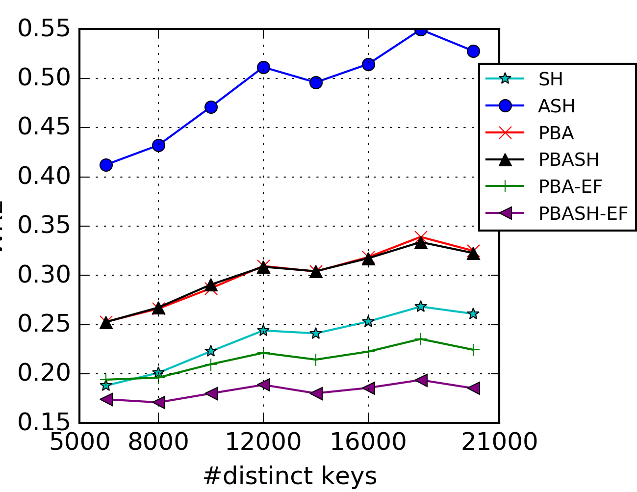
Figure 2 illustrates error metrics for PBA, PBASH, and ASH in a reservoir of size $m=1,000$ processing items from the synthetic Trace 1. The number of distinct keys varies from 6,000 to 20,000, representing a key sampling rate ranging from $17\%$ down to $5\%$, WRE was reduced, relative to ASH, by about 40% for PBA and PBASH, by 53–57% for PBA-EF, and by 58–65% for PBASH-EF. As shown, PBASH and PBASH-EF are able to achieve lower WRE than a best-case (non-adaptive) Sample and Hold (SH) in which the sampling rate is chosen so as minimize WRE.

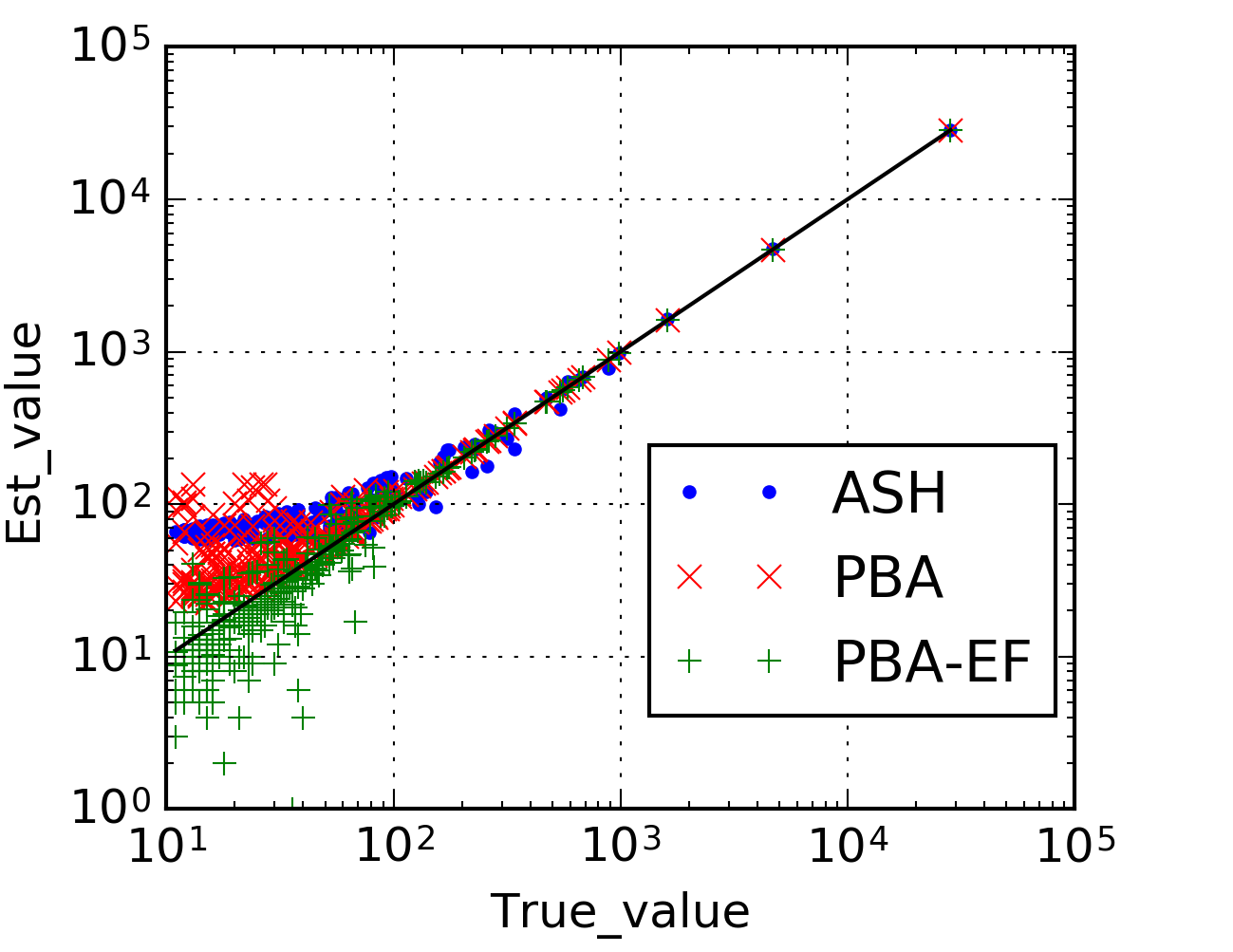
To better understand the difference in error between PBA, PBA-EF and ASH, we drill down within an individual experiment. Figure 2 is a scatter plot of estimated vs. true aggregate for the two methods for a synthetic trace containing $10^{4}$ distinct keys sampled into a reservoir of size $500$, i.e., a key sampling rate of $5\%$. The figure shows how PBA improves estimation accuracy for smaller weight keys, ASH having a larger additive error (note the logarithmic vertical axis). As expected, PBA-EF further reduces the estimation error for small aggregates, typically underestimating the true value.

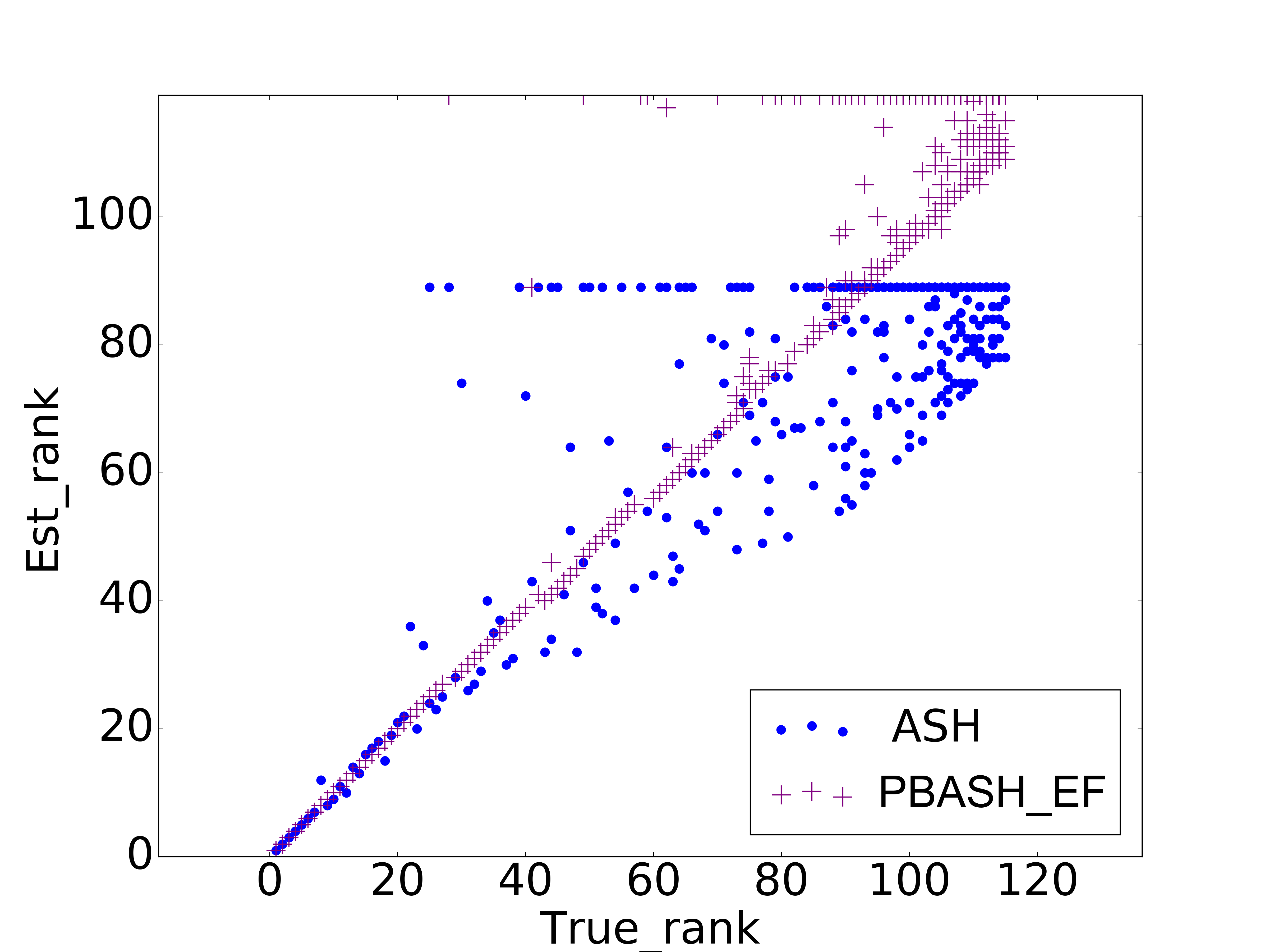
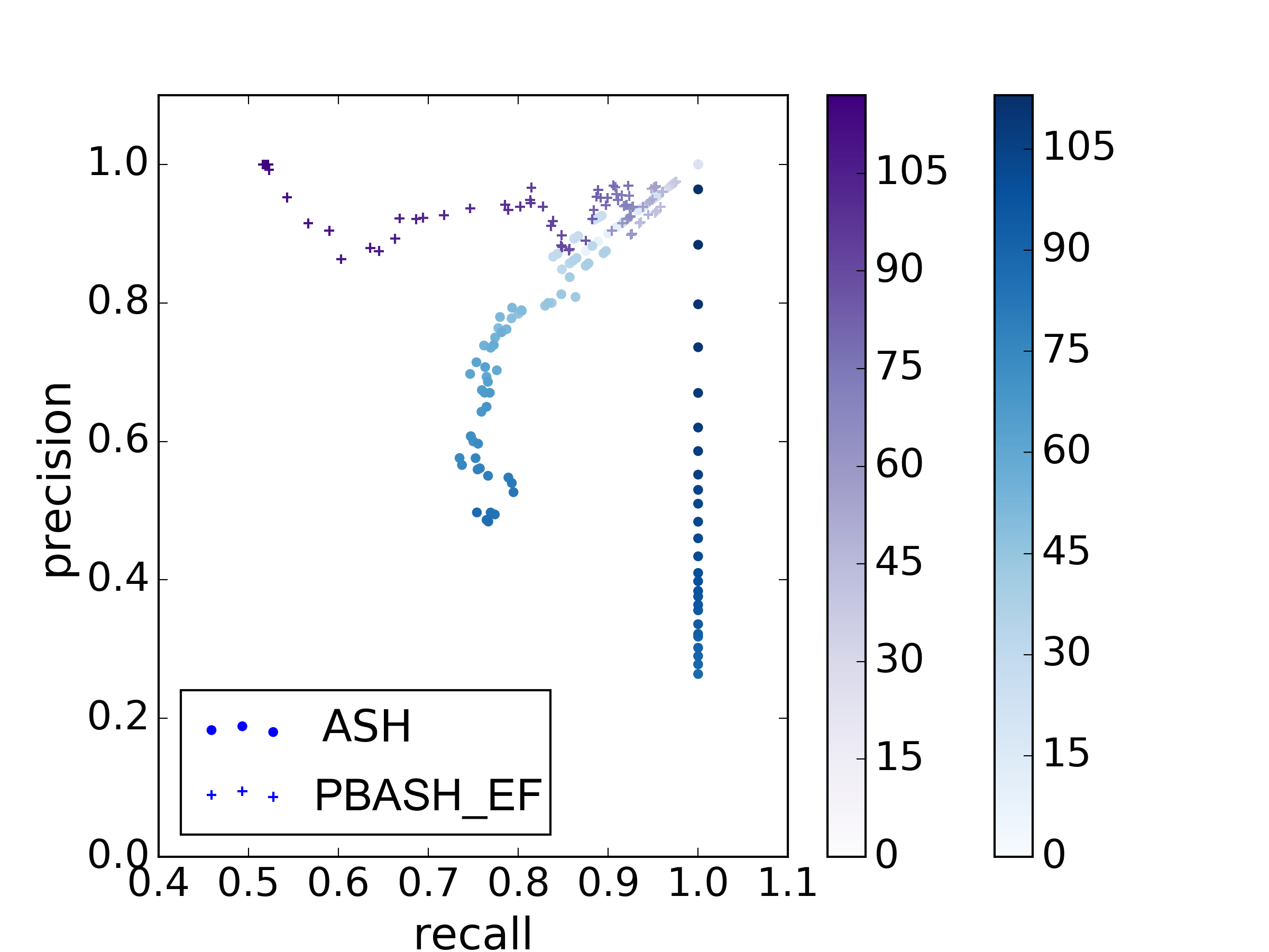
Rank Estimation. We evaluate rank estimation performance, focusing on algorithms involving Error Filtering since rankings should be less sensitive to bias than variability. Figure 4 shows a scatter plot of estimates vs. actual dense ranks at 5% sampling for PBASH-EF and ASH. Although both perform well for low ranks (larger aggregates), we observe increasing rank noise for ASH in mid to low ranks. The horizontal clusters in each case correspond to aggregates not sampled; there are noticeably more of these of lower true rank for ASH than PBA-EF. Figure 4 shows precision and recall for top-$R$ rank queries. Precision is noticeably better for PBASH-EF, particularly for middle ranks.

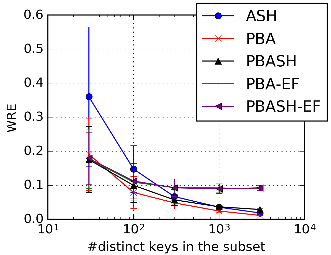
Subpopulation Weight Estimation. Figure 6 shows WRE for subpopulations over 100 random selected subpopulations as a function of subpopulation size. For small subpopulations up to size 100, PBA and derived methods provide up to about a 60% reduction in WRE relative to ASH. The WREs of the unbiased methods (PBA, PBASH, ASH) behave similarly for larger subpopulation sizes due to averaging, while the bias of the error filtering methods persist.

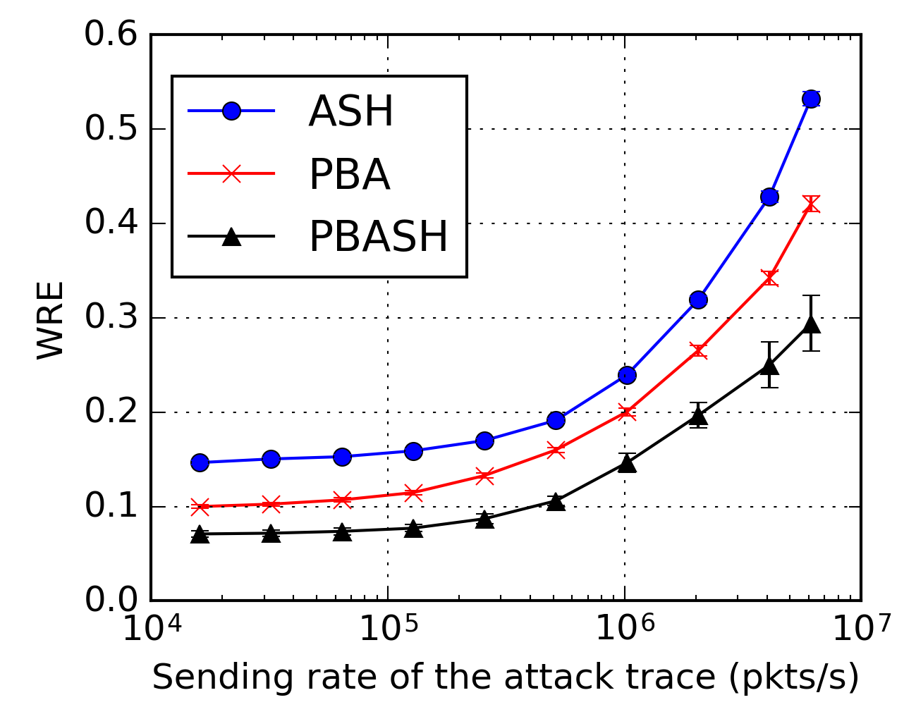
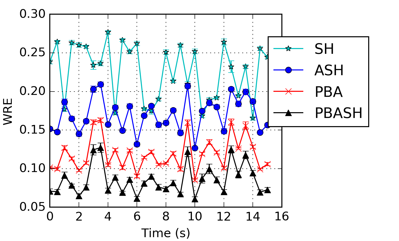
Network dynamics. We study the effect in accuracy on an emulated DDoS attack with Trace 2. Figure 6 shows the effect on WRE as the DDoS traffic rate increases, in a reservoir of size 5,000. The number of distinct keys increases in proportion to the attack traffic rate, with legitimate traffic representing a smaller proportion of the total. PBA and PBASH achieve lower error than ASH, even as errors for all methods increase, and PBASH-EF (not shown) achieves 60% reduction in error compared with ASH. Figure 8 shows a time series of WRE for the dynamic traffic of Trace 3, with samples taken over successive 250ms windows in a reservoir size 5,000. PBA and PBASH have smaller fluctuations in WRE in response to the dynamics than ASH  achieving similar reduction as before.

Figure 7. The impact of traffic dynamics by adding random noise when the reservoir size is $5,000$.

Figure 8. The time complexity compared to ASH with varying reservoir sizes and $10^{4}$ distinct keys.

Figure 9. The number of insertions when the reservoir size is from $100$ to $1,000$.

6.3. Computational Complexity

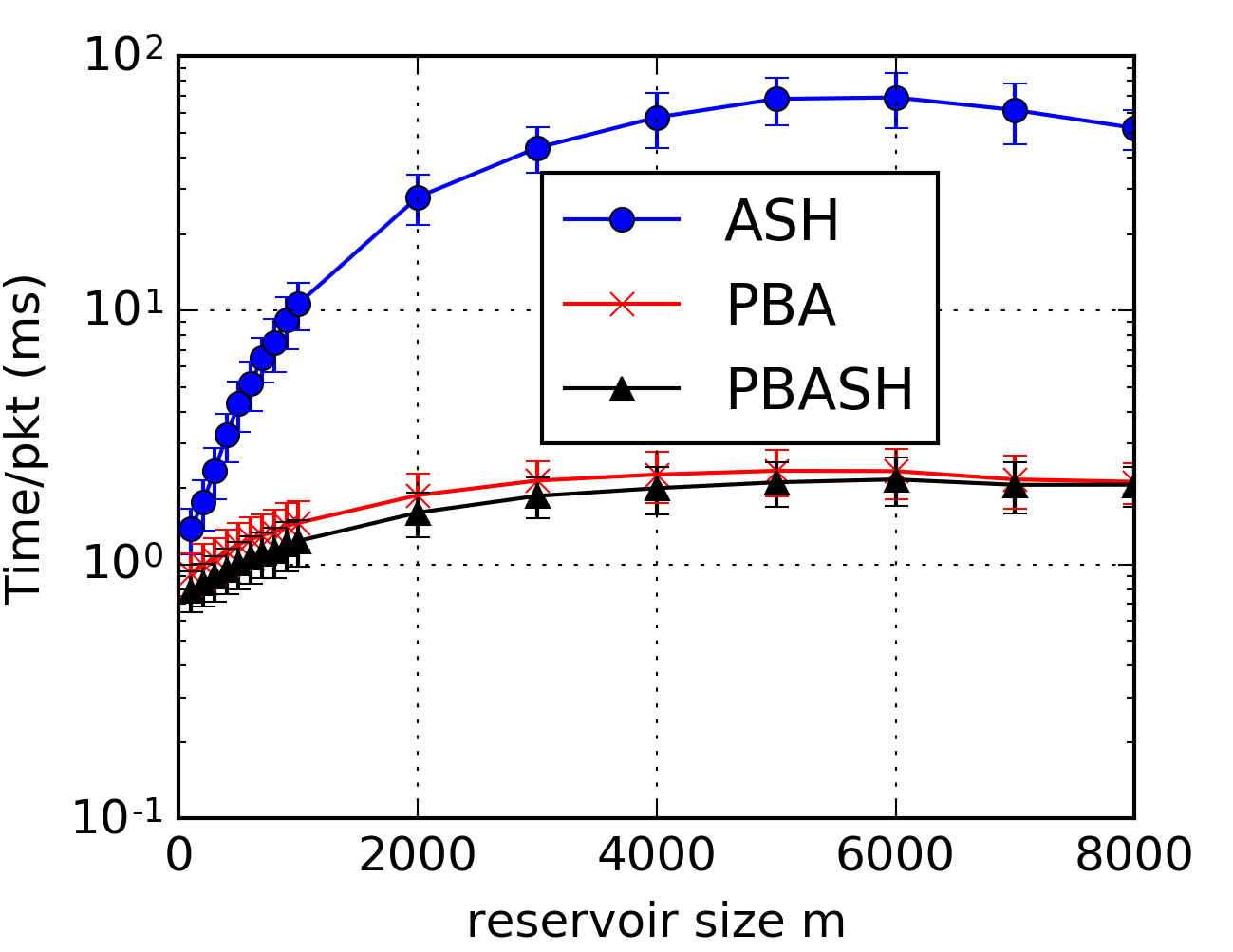
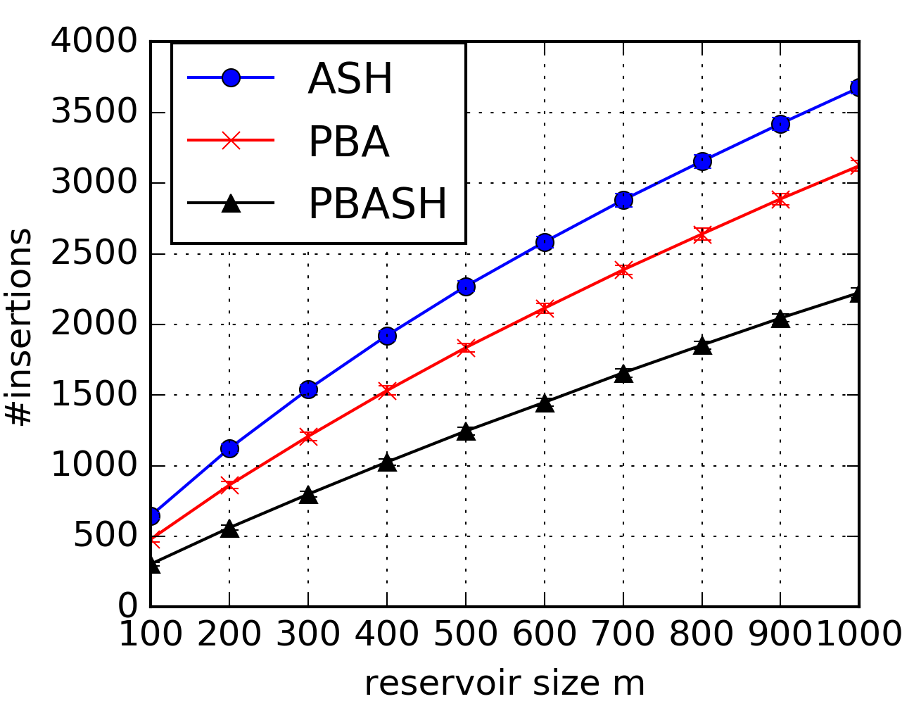
Figure 8 shows the processing time per packet of PBA, PBASH and ASH. No optimizations of ASH were used beyond the specification in (Cohen, 2015). With this proviso, the $O(m)$ cost for key eviction from reservoir size $m$ for ASH appears evident through the initial linear growth of the time per packet. The noticeably lower growth for PBA and PBASH are expected due to its $O(\log m)$ time for inserting a new key after eviction of a current key. Since insertion/eviction is the most costly part for all algorithms we display the experimental number of these for each algorithm in Figure 9. PBASH has about half the insertions of ASH, another factor in its smaller per packet time. PBASH also has a smaller number of insertions than PBA. This is to be expected, since the PBASH pre-sampling stages causes fewer keys to be admitted to the reservoir.

7. Conclusions

Weighted sample-based algorithms are a flexible approach to stream summarization, whose outputs can be readily utilized by downstream applications for queries on ranks and subpopulations. This paper provides a new set of algorithms, Priority-Based Aggregation and its variants) of this type. PBA is designed around a single random variable per key aggregate, allowing considerable speed-up in a fixed cache, and it also improves accuracy for a given sample size, compared with state-of-the-art methods.

8. Proofs of the Theorems

Proof of Theorem 3.1.

For each $k$ we proceed by induction on $t\geq s_{k}=\min\{s:k_{s}=k\}$ and establish that

(11) $${\mathbb{E}}[\widehat{X}_{k,t}|\widehat{X}_{k,t-1},C]-X_{k,t}=\widehat{X}_{k,t-1}-X_{k,t-1}$$

for all members $C$ of a covering partition (i.e., a set of disjoint events whose union is identically true). Since $\widehat{X}_{k,s_{k}-1}=X_{k,s_{k}-1}=0$ we conclude that ${\mathbb{E}}[\widehat{X}_{k,t}]=X_{k,t}$.

For $s_{k}\leq s\leq s^{\prime}$ let $A_{k}(s)=\{k\notin\widehat{K}_{s-1}\}$ (note $A_{k}(s_{k})$ is identically true), let $B_{k}(s,s^{\prime})$ denote the event $\{k\in\widehat{K}_{s}\dots,\widehat{K}_{s^{\prime}}\}$, i.e., that $k$ is in sample at all times in $[s,s^{\prime}]$ . Then for each $t\geq s_{k}$ the collection of events formed by $\{A_{k}(s)B_{k}(s,t-1):\ s\in[s_{k},t-1]\}$, and $A_{k}(t)$ is a covering partition.

(i) Conditioning on $A_{k}(t)$ On $A_{k}(t)$, $k_{t}\neq k$ implies $\widehat{X}_{k,t}=\widehat{X}_{k,t-1}=0=X_{k,t}-X_{k,t-1}$. On the other hand $k_{t}=k$ implies $t\in T^{0}$. Further conditioning on $z_{k,t}=\min_{j\in\widehat{K}_{j,t-1}}W_{j,t-1}/u_{j}$ then (8) tells us that

(12) $${\mathbb{P}}[k\in\widehat{K}_{t}|A_{k}(t),z_{k,t}]={\mathbb{P}}[W_{k,t}/u_{k}\leq z_{k,t}]=q_{k,t}$$

and hence regardless of $z_{k,t}$ we have

(13) $${\mathbb{E}}[\widehat{X}_{k,t}|X_{k,t-1},A_{k}(t),z_{k,t}]=\widehat{X}_{k,t-1}+X_{k,t}-X_{k,t-1}$$

(ii) Conditioning on $A_{k}(s)B_{k}(s,t-1)$ any $s\in[s_{k},t-1]$. Under this condition $k\in\widehat{K}_{t-1}$ and if furthermore $k_{t}\in\widehat{K}_{t-1}$ then $t\notin T^{0}$ and the first line in (8) holds. Suppose instead $k_{t}\notin K_{t-1}$ so that $t\in T^{0}$. Let ${\mathcal{Z}}_{k}(t,s)=\{z_{k,r}:r\in[s,t]^{0}\}$. Observing that

$${\mathbb{P}}[B_{k}(t,s)|A_{k}(s),{\mathcal{Z}}_{k}(t,s)]={\mathbb{P}}[\cap_{r\in[s,t]^{0}}\{z_{k,r}\leq\frac{W_{k,r}}{u_{k}}\}]=q_{k,t}$$

then

$$\kern-40.0pt{\mathbb{P}}[k\in\widehat{K}_{t}|B_{k}(t-1,s)A_{k}(s),{\mathcal{Z}}_{k}(t,s)]$$

$$= \frac{{\mathbb{P}}[B_{k}(t,s)|A_{k}(s),{\mathcal{Z}}_{k}(t,s)]}{{\mathbb{P}}[B_{k}(t-1,s)|A_{k}(s),{\mathcal{Z}}_{k}(t-1,s)]}=\frac{q_{k,t}}{q_{k,\tau_{t}}}=Q_{k,t}$$

and hence

(15) $${\mathbb{E}}[\widehat{X}_{k,t}|\widehat{X}_{k,t-1},A_{k}(s),{\mathcal{Z}}_{k}(t,s)]=\widehat{X}_{k,t-1}$$

independently of the conditions on the LHS of (15). AS noted above, $k\in\widehat{K}_{t-1}$ on $B(t-1,s)$ hence $X_{k,t}=X_{k,t-1}$ and we recover (11). Since we now established (11) over all members $C$ of a covering partition, the proof is complete. ∎

Proof of Theorem 4.1.

$t\in T$ means the arriving $k_{t}\neq d_{t}$ is admitted to the reservoir and hence

(16) $$z_{t}=\frac{W_{d_{t},t}}{u_{d_{t}}}\geq\frac{W_{d_{t},s}}{u_{d_{t}}}\geq z_{s}$$

for all $s\in[\tau_{d_{t},t},t]^{0}$. The first inequality follows because $W_{d_{t},s}$ is nondecreasing on the interval $[\tau_{d_{t},t},t]^{0}$. The second inequality follows because the key $d_{t}$ survives selection throughout $[\tau_{d_{t},t},t]^{0}$ and hence its priority cannot be lower than the threshold $z_{s}$ for any $s$ in that interval. Since $d_{t}$ was admitted at $\tau_{d_{t},t}$, then $d_{\tau_{d_{t},t}}\neq d_{t}$ and hence we apply the argument back recursively to the first sampling time $m+1$. This establishes $z_{t}\geq z^{*}_{t}$ and hence $z_{t}=z_{t}^{*}$.

(ii) $i$ is admitted to $\widehat{K}_{t}$ if $t\in T$ with $i=k_{t}\neq d_{t}$ and hence by (i), $q_{i,t}=\min\{1,W_{i,t}/z_{t}\}=\min\{1,w_{i,i}/z^{*}_{t}\}=q^{*}_{i,t}$. We establish the general case by induction. Assume $t\in T^{0}$ and $q_{i,s}=q^{*}_{i,s}$ for all $s\in[\tau_{i,t},\tau_{t}]^{0}$, and consider first the case that $z_{t}>z^{*}_{\tau_{t}}t$. Then $z^{*}_{t}=z_{t}$ hence $q^{*}_{i,t}=q_{i,t}$. If instead $z_{t}\leq z^{*}_{\tau_{t}}$ then $z^{*}_{\tau_{t}}=z^{*}_{t}$ and

(17) $$\frac{W_{i,t}}{z_{t}}\geq\frac{W_{i,t}}{z^{*}_{t}}\geq\frac{W_{i,\tau_{t}}}{z^{*}_{t}}=\frac{W_{i,\tau_{t}}}{z^{*}_{t}}$$

Thus we can replace $z_{t}$ by $z^{*}_{t}$ but use of either leaves the iterated value unchanged, since by the induction hypothesis, both are greater than $q_{i,\tau_{t}}\leq W_{i,\tau_{t}}/z^{*}_{i,\tau_{t}}$ ∎

References

- (1)
- Ahmed et al. (2014) Nesreen K. Ahmed, Nick G. Duffield, Jennifer Neville, and Ramana Rao Kompella. 2014. Graph Sample and Hold: A Framework for Big-Graph Analytics. In ACM SIGKDD.
- Ahmed et al. (2017) Nesreen K. Ahmed, Nick G. Duffield, Theodore L. Willke, and Ryan A. Rossi. 2017. On Sampling from Massive Graph Streams. PVLDB 10, 11 (August 2017).
- Alon et al. (1999) N. Alon, Y. Matias, and M. Szegedy. 1999. The Space Complexity of Approximating the Frequency Moments. J. Comput. System Sci. 58, 1 (1999), 137–147.
- Andoni et al. (2010) Alexandr Andoni, Robert Krauthgamer, and Krzysztof Onak. 2010. Streaming Algorithms from Precision Sampling. Technical Report 1011.1263. arXiv.
- Andreyev (2014) Alexey Andreyev. 2014. Introducing data center fabric, the next-generation Facebook data center network. (2014). https://code.facebook.com/posts/360346274145943/introducing-data-center-fabric-the-next-generation-facebook-data-center-network/.
- Braverman and Ostrovsky (2010) Vladimir Braverman and Rafail Ostrovsky. 2010. Zero-one Frequency Laws (STOC ’10). ACM, New York, NY, USA, 281–290.
- CAIDA (2012) CAIDA. 2012. CAIDA Anonymized Internet Traces. (2012). http://www.caida.org/data/passive/passive_2012_dataset.xml.
- Cisco Systems (2012) Cisco Systems. 2012. Introduction to Cisco IOS NetFlow - A Technical Overview. http://www.cisco.com/c/en/us/products/collateral/ios-nx-os-software/ios-netflow/prod_white_paper0900aecd80406232.html. (2012).
- Cohen (2015) Edith Cohen. 2015. Stream Sampling for Frequency Cap Statistics. In ACM SIGKDD. New York, NY, USA, 159–168.
- Cohen et al. (2012) Edith Cohen, Graham Cormode, and Nick Duffield. 2012. Don’t let the negatives bring you down: sampling from streams of signed updates. In SIGMETRICS 40, 1 (2012), 343–354.
- Cohen et al. (2007) Edith Cohen, Nick Duffield, Haim Kaplan, Carsten Lund, and Mikkel Thorup. 2007. Algorithms and Estimators for Accurate Summarization of Internet Traffic. In Proceedings of the 7th ACM SIGCOMM Conference on Internet Measurement (IMC ’07). ACM, New York, NY, USA, 265–278.
- Cohen and Kaplan (2007) E. Cohen and H. Kaplan. 2007. Summarizing data using Bottom-k sketches. In Proceedings of the ACM PODC’07 Conference.
- Cohen and Kaplan (2008) E. Cohen and H. Kaplan. 2008. Tighter estimation using bottom-k sketches. In Proceedings of the 34th VLDB Conference. http://arxiv.org/abs/0802.3448
- Cormode and Muthukrishnan (2004) Graham Cormode and S. Muthukrishnan. 2004. An improved data stream summary: The Count-Min sketch and its applications. J. Algorithms 55 (2004), 29–38.
- Cranor et al. (2003) Chuck Cranor, Theodore Johnson, Oliver Spatscheck, and V ladislav Shkapenyuk. 2003. Gigascope: A Stream Database for Network Applications. In Proc ACM SIGMOD.
- Duffield and Krishnamurthy (2016) N. Duffield and B. Krishnamurthy. 2016. Efficient sampling for better OSN data provisioning. In 2016 54th Annual Allerton Conference on Communication, Control, and Computing (Allerton). 861–868.
- Duffield et al. (2007) N. Duffield, M. Thorup, and C. Lund. 2007. Priority sampling for estimating arbitrary subset sums. J. Assoc. Comput. Mach. 54, 6 (2007).
- Efraimidis and Spirakis (2006) P. S. Efraimidis and P. G. Spirakis. 2006. Weighted random sampling with a reservoir. Inf. Process. Lett. 97, 5 (2006), 181–185.
- Estan and Varghese (2002) Cristian Estan and George Varghese. 2002. New Directions in Traffic Measurement and Accounting. In Proc. of SIGCOMM. 323–336.
- Feldmann et al. (1998) Anja Feldmann, Jennifer Rexford, and Ramon Caceres. 1998. Efficient policies for carrying Web traffic over flow-switched networks. IEEE/ACM Transactions on Networking (December 1998), 673–685.
- Gibbons and Matias (1998) P. Gibbons and Y. Matias. 1998. New sampling-based summary statistics for improving approximate query answers. In SIGMOD. ACM.
- Gilbert et al. (2002) Anna C. Gilbert, Sudipto Guha, Piotr Indyk, Yannis Kotidis, S. Muthukrishnan, and Martin J. Strauss. 2002. Fast, Small-space Algorithms for Approximate Histogram Maintenance (STOC ’02). ACM, New York, NY, USA, 389–398.
- Hájek (1960) J. Hájek. 1960. Limiting Distributions in Simple Random Sampling from a Finite Population. Publications of Mathematical Institute of Hungarian Academy of Sciences, Series A 5 (1960), 361–374.
- Indyk (2000) P. Indyk. 2000. Stable Distributions, Pseudorandom Generators, Embeddings and Data Stream Computation. In Proc. of the 41st Symposium on Foundations of Computer Science.
- Johnson et al. (1986) William B. Johnson, Joram Lindenstrauss, and Gideon Schechtman. 1986. Extensions of lipschitz maps into Banach spaces. Israel Journal of Mathematics 54, 2 (1986), 129–138. DOI:http://dx.doi.org/10.1007/BF02764938
- Jowhari et al. (2011) Hossein Jowhari, Mert Saglam, and Gábor Tardos. 2011. Tight bounds for Lp samplers, finding duplicates in streams, and related problems. In PODS. 49–58.
- Keys et al. (2005) K. Keys, D. Moore, and C. Estan. 2005. A robust system for accurate real-time summaries of internet traffic. ACM SIGMETRICS Performance Evaluation Review 33 (2005).
- Li et al. (2016) Yuliang Li, Rui Miao, Changhoon Kim, and Minlan Yu. 2016. FlowRadar: a better NetFlow for data centers. In 13th USENIX Symposium on Networked Systems Design and Implementation (NSDI 16). USENIX Association, 311–324.
- Liu et al. (2016a) Xiufeng Liu, Lukasz Golab, Wojciech Golab, Ihab F. Ilyas, and Shichao Jin. 2016a. Smart Meter Data Analytics: Systems, Algorithms, and Benchmarking. ACM Trans. Database Syst. 42, 1, Article 2 (November 2016), 39 pages.
- Liu et al. (2016b) Zaoxing Liu, Antonis Manousis, Gregory Vorsanger, Vyas Sekar, and Vladimir Braverman. 2016b. One Sketch to Rule Them All: Rethinking Network Flow Monitoring with UnivMon. In Proceedings of the 2016 Conference on ACM SIGCOMM 2016 Conference (SIGCOMM ’16). ACM, New York, NY, USA, 101–114.
- Lo et al. (2016) Caroline Lo, Dan Frankowski, and Jure Leskovec. 2016. Understanding Behaviors That Lead to Purchasing: A Case Study of Pinterest. In Proceedings of the 22Nd ACM SIGKDD International Conference on Knowledge Discovery and Data Mining (KDD ’16). ACM, New York, NY, USA, 531–540.
- Metwally et al. (2005) Ahmed Metwally, Divyakant Agrawal, and Amr El Abbadi. 2005. Efficient Computation of Frequent and Top-k Elements in Data Streams. In Proceedings of the 10th International Conference on Database Theory (ICDT’05). Springer-Verlag, Berlin, Heidelberg, 398–412.
- Monemizadeh and Woodruff (2010) M. Monemizadeh and D. P. Woodruff. 2010. 1-Pass Relative-Error L-Sampling with Applications. In Proc. 21st ACM-SIAM Symposium on Discrete Algorithms. ACM-SIAM.
- Moshref et al. (2015) Masoud Moshref, Minlan Yu, Ramesh Govindan, and Amin Vahdat. 2015. SCREAM: Sketch Resource Allocation for Software-defined Measurement. In Proceedings of the 11th ACM Conference on Emerging Networking Experiments and Technologies (CoNEXT ’15). ACM, New York, NY, USA, Article 14, 13 pages.
- Pǎtraşcu and Thorup (2012) Mihai Pǎtraşcu and Mikkel Thorup. 2012. The Power of Simple Tabulation Hashing. J. ACM 59, 3, Article 14 (June 2012), 50 pages.
- Rosén (1972) B. Rosén. 1972. Asymptotic Theory for Successive Sampling with Varying Probabilities Without Replacement, I. The Annals of Mathematical Statistics 43, 2 (1972), 373–397. http://www.jstor.org/stable/2239977
- Rosén (1997) B. Rosén. 1997. Asymptotic theory for order sampling. J. Statistical Planning and Inference 62, 2 (1997), 135–158.
- Roy et al. (2015) Arjun Roy, Hongyi Zeng, Jasmeet Bagga, George Porter, and Alex C Snoeren. 2015. Inside the social network’s (datacenter) network. In ACM SIGCOMM Computer Communication Review, Vol. 45. ACM, 123–137.
- Vitter (1985) J. Vitter. 1985. Random sampling with a reservoir. ACM Trans. Math. Softw. 11 (1985). Issue 1.
- Williams (1991) David Williams. 1991. Probability with Martingales. Cambridge University Press.
- Yu et al. (2013) Minlan Yu, Lavanya Jose, and Rui Miao. 2013. Software Defined Traffic Measurement with OpenSketch. In Proceedings of the 10th USENIX Conference on Networked Systems Design and Implementation (nsdi’13). USENIX Association, Berkeley, CA, USA, 29–42. http://dl.acm.org/citation.cfm?id=2482626.2482631