A Unifying Bayesian Optimization Framework for Radio Frequency Localization

Abstract

We consider the problem of estimating an RF-device’s location based on observations, such as received signal strength, from a set of transmitters with known locations. We survey the literature on this problem, showing that previous authors have considered implicitly or explicitly various metrics. We present a novel Bayesian framework that unifies these works and shows how to optimize the location estimation with respect to a given metric. We demonstrate how the framework can incorporate a general class of algorithms, including both model-based methods and data-driven algorithms such fingerprinting. This is illustrated by re-deriving the most popular algorithms within this framework. When used with a data-driven approach, our framework has cognitive self-improving properties in that it provably improves with increasing data compared to traditional methods. Furthermore, we propose using the error-CDF as a unified way of comparing algorithms based on two methods: (i) stochastic dominance, and (ii) an upper bound on error-CDFs. We prove that an algorithm that optimizes any distance based cost function is not stochastically dominated by any other algorithm. This suggests that in lieu of the search for a universally best localization algorithm, the community should focus on finding the best algorithm for a given well-defined objective.

I Introduction

The ability to locate a wireless device based on received signal strength from known-location transmitters is of great utility for many applications, including indoor location-based mobile apps and services, interactive media, emergency search and rescue, asset tracking, etc. A significant number of researchers have tackled this fundamental problem and proposed various algorithms for radio signal strength (RSS) based localization. Many works adopt standard algorithms from signal processing, specifically estimation theory, such as Maximum Likelihood Estimation [1], Minimum Mean Squared Error Estimation [2], Best Linear Unbiased Estimator [3], etc., while other techniques such as finger-printing [4], and sequence-based localization [5], are somewhat more heuristically derived. These algorithms are typically evaluated using numerical and trace-based simulations, using varied metrics such as the mean squared position error, the absolute distance error, etc.

We contend that the literature is disconnected and disorganized and that it is hard to decipher any unified theory that fairly evaluates these algorithms across different metrics of interest. We argue that the state-of-the-art approach to localization in the literature — which typically involves first presenting an algorithm and then evaluating its performance according to a particular metric or a set of metrics — is akin to putting the proverbial cart before the horse. For instance, it is not uncommon for algorithms to be evaluated on metrics for which they are not explicitly or implicitly optimized.

We advocate a systematic way of designing location estimation algorithms which we refer to as the “optimization-based approach to localization”. In this approach, first the localization metric is defined in terms of a suitable cost function, then an appropriate estimation algorithm is derived to minimize that cost function. In addition, our optimization framework is applicable to any deterministic or stochastic model of the observations (assumed to be known) and can accommodate any prior distribution for location. Our framework also applies to data-driven approaches such as fingerprinting. We show that, in such data-driven settings, our framework (i) makes better use of the available data, and (ii) has cognitive self-improving properties in that it provably gets better with increasing data compared to traditional methods. Fundamentally a Bayesian approach, this framework is also compatible with Bayesian filtering for location tracking over time [6].

As an illustration of our framework, we consider first a common metric used in the evaluation of localization algorithms, the absolute distance error, and derive an algorithm which yields location estimates so as to minimize the expected distance error (MEDE). For a second illustration, we also consider as another metric the probability that the location estimate is within a given radius of the true location ($P(d)$) and derive an algorithm which maximizes this probability. Furthermore, we show that standard algorithms such as MLE and MMSE can be derived similarly from optimizing the corresponding metrics (likelihood, mean squared error respectively).

In conjunction with our framework for deriving algorithms to optimize a specified metric, we also consider the problem of comparing different localization algorithms with each other; for which we propose the use of the error CDF. For an important class of cost functions that can be expressed as non-negative monotonically increasing functions of distance error, we prove that there is in effect a partial ordering among various estimation algorithms. Certain algorithms dominate other algorithms for all such cost functions, and we show the necessary condition for this to happen. But there could also be two algorithms, $A_{1}$ and $A_{2}$, and two metrics, $M_{1}$ and $M_{2}$, such that $A_{1}$ is better than $A_{2}$ in terms of $M_{1}$ while the reverse is true for $M_{2}$. Thus we show that there is, in general, no single-best localization algorithm, but rather a “Pareto Set” of algorithms that are each optimized for different cost functions.

We evaluate the optimization-based framework for location estimation using both numerical simulations, traces [7], and data obtained from experiments in an indoor office environment. We illustrate how our framework can incorporate a variety of localization algorithms, including fingerprinting based methods. Our evaluation confirms what is predicted by the theory — no single algorithm outperforms others with respect to all metrics, thus underlining the need for an optimization based apporach such as the one we propose.

I-A Contributions

• We propose a novel optimization-based Bayesian framework that unifies and puts in context various previously proposed techniques for localization and provides a systematic basis for developing new algorithms.

• We demonstrate the usage of error CDF as a unifying mathematical abstraction for evaluating the performance of a localization algorithm. We first introduce a partial ordering over the set of algorithms by considering a stochastic dominance relationship between their error CDFs. We prove that any algorithm that optimizes a distance based cost function is not stochastically dominated by any other algorithm.

• We further demonstrate a second way of evaluating and comparing algorithms based on how ‘close’ an algorithm gets to the upper bound on error CDFs. We propose one such measure of closeness (area of difference) and identify MEDE as the optimal algorithm over that measure.

• We illustrate how our framework encompasses both model-based approaches and data-driven methods such as fingerprinting, through simulations and real-world experiments.

The rest of the paper is organized as follows: A survey of the existing literature on RSS based localization algorithms is given in Section II. We introduce our optimization based localization framework in Section III. In Section IV we introduce the concept of stochastic dominance and prove how it leads to a partial ordering over the set of localization algorithms. We also introduce the upper bound on error CDFs and illustrate the evaluation of algorithms using the same. In Section V we evaluate our framework using simulations and trace data. We also show how fingerprinting methods fit into our framework. We conclude in Section VI.

II Literature on RSS based Localization

TABLE I: Literature Survey on Localization Methods

Study	Algorithm	Model	Metric
WLAN location determination via clustering and probability distributions [8]	MLE	Fingerprinting	$P(d)$
Maximum likelihood localization estimation based on received signal strength [1]	MLE	Log-Normal	MSE
Experimental comparison of RSSI-based localization algorithms for indoor wireless sensor networks [9]	Multilateration and MLE	Log-Normal	EDE
A Bayesian sampling approach to in-door localization of wireless devices using RSSI [10]	Weighted MLE and Error CDF	Fingerprinting	EDE
RADAR: An In-Building RF-based user location and tracking system [4]	Clustering	Fingerprinting	EDE
The Horus WLAN location determination system [11]	MLE	Fingerprinting	EDE
Locating in fingerprint space: Wireless indoor localization with little human intervention [12]	Clustering	Fingerprinting	EDE
Weighted centriod localization in Zigbee-based sensor networks [13]	RSSI weighted position	Free Space Path Loss	EDE
Sequence based localization in wireless sensor networks [5]	SBL	Free Space Path Loss	EDE
Best linear unbiased estimator algorithm for RSS based localization [3]	Best linear unbiased estimate	Log-Normal	MSE
Performance of an MMSE based indoor localization with wireless sensor networks [2]	MMSE	Log-Normal	MSE
Relative location estimation in wireless sensor networks [14]	MLE	Log-Normal	MSE
Distance Estimation from RSS under log-normal shadowing [15]	Best unbiased estimate	Log-Normal	MSE

In this section, we survey the existing literature on RSS based localization algorithms with the intention of comparing, across papers, the metrics used to evaluate the algorithms. The results of the survey are summarized in Table I. We identify certain metrics that are commonly used across the literature:

• MSE: Mean Squared Error is the expected value of the square of the Euclidean distance between our estimate and the true location. Often the square root of this quantity Root Mean Squared Error (RMSE) is given instead of MSE. As RMSE may be derived using MSE, we shall only use MSE in our discussions in this paper. The minimum mean squared error (MMSE) algorithm returns an estimate that minimizes the MSE.

• EDE: The Expected Distance Error (EDE) is the expected value of the Euclidean distance between our estimate and the true location. The minimum expected distance error (MEDE) algorithm returns an estimate that minimizes the EDE.

• $P(d)$: $P(d)$ indicates the probability that the receiver location is within a distance of $d$ from our location estimate. $P(d)$ is closely related to the metric $D(p)$ which gives the radius at which an open ball around our location estimate yields a probability of at least $p$. The M$P(d)$ algorithm returns an estimate that minimizes the $P(d)$.

As evidenced by Table I, it is with striking regularity that one encounters a mismatch between an algorithm and the metric used for its evaluation. While there is hardly anything amiss in checking how an algorithm performs on a metric that it is not optimized for, it is shortsighted to draw a conclusion as to the efficacy of the said algorithm based on such an evaluation. An awareness of the metric that an algorithm is implicitly or explicitly optimized for, is essential to its fair assessment. We believe that such of notion of consistent evaluation of algorithms across all important metrics of interest has been absent in the community so far. In addition while the literature on localization abounds in algorithms that yield a location estimate, there is no unifying theory that relates them to each other with appropriate context.

For instance, [16] picks four algorithms for evaluation, indepedent of the metrics used to evaluate the algorithms. Such an approach makes it unclear if an algorithm is optimal with respect with any of the given metrics. In this case, we can only make (empirical) inferences regarding the relative ordering of the chosen algorithms among the chosen metrics. Consequently, there are no theoretical guarentees on algorithm performance and it becomes hard, if not impossible, to accurately predict how a chosen algorithm will behave when evaluated with a metric that was not considered.

Moreover, while error CDFs have been used earlier to compare algorithms [17], they are typically used to derive inferences about algorithm performance with respect to the Euclidean distance and $D(p)$ metrics. In the absence of the unifying theory presented in this proposal, it is unclear how one may draw meaningful conclusions regarding the relative performance of algorithms across various metrics based on their error CDF. Our proposed unifying framework places the commonly employed subjective reading of error CDFs on a firm theoretical footing and enables a better understanding of algorithm performance than what was previously possible. Moreover, our framework is computationally tractable as the optimization is typically done over a reasonably sized discrete set of possible locations.

Table I also indicates that there is considerable interest in the community for the EDE metric. However, it is interesting to note that none of the algorithms evaluated using that metric are explicitly optimized for it. In the following sections we show how such metrics fit into our framework. More importantly, it is our hope that thinking in terms of the framework below shall lead to a clearer understanding of the trade-offs involved in choosing an algorithm and a better specification of the criterion necessary for its adoption.

Figure 1: Localization Algorithms

The optimization-based framework for localization presented in this paper is inspired in part by the optimization-based approach to networking developed since the late 90’s [18], which has shown successfully that efficient medium access, routing, and congestion control algorithms, protocols, and architectures all can be derived from suitably specified network utility maximization problems [19]. Moreover, Bayesian optimization is increasingly gaining in popularity in the recent years [20], including applications in cognitive radio networks [21, 22], largely due to the increased availability of both abundant data and the computational power needed to process that data. Our proposed framework is poised to leverage both these trends.

III A Unifying Framework for Deriving Localization Algorithms

TABLE II: Recovering existing algorithms in our framework

Algorithm	Cost function	Optimization
MMSE	$\mathcal{C}({\bm{r}},\tilde{{\bm{r}}},{\bm{o}})={\left(\|\tilde{{\bm{r}}}-{\bm{r}}\|_{2}\right)}^{2}$	${{\bm{r}}}_{MMSE}=\operatorname*{arg\,min}_{\tilde{{\bm{r}}}}\operatorname*{\mathrm{E}}\left[{\left(\|\tilde{{\bm{r}}}-{\bm{r}}\|_{2}\right)}^{2}\right]$
MEDE	$\mathcal{C}({\bm{r}},\tilde{{\bm{r}}},{\bm{o}})=\|\tilde{{\bm{r}}}-{\bm{r}}\|_{2}$	${{\bm{r}}}_{MEDE}=\operatorname*{arg\,min}_{\tilde{{\bm{r}}}}\operatorname*{\mathrm{E}}\left[\|\tilde{{\bm{r}}}-{\bm{r}}\|_{2}\right]$
M$P(d)$	$\mathcal{C}({\bm{r}},\tilde{{\bm{r}}},{\bm{o}})=-P\left(\|\tilde{{\bm{r}}}-{\bm{r}}\|_{2}\leq d\right)$	${{\bm{r}}}_{MP(d)}=\operatorname*{arg\,max}_{\tilde{{\bm{r}}}}\operatorname*{\mathrm{E}}\left[P\left(\|\tilde{{\bm{r}}}-{\bm{r}}\|_{2}\leq d\right)\right]$
MLE	$\mathcal{C}({\bm{r}},\tilde{{\bm{r}}},{\bm{o}})=-P\left(\|\tilde{{\bm{r}}}-{\bm{r}}\|_{2}\leq\epsilon\right)$	${{\bm{r}}}_{MLE}=\lim_{\epsilon\to 0}\operatorname*{arg\,max}_{\tilde{{\bm{r}}}}\operatorname*{\mathrm{E}}\left[P\left(\|\tilde{{\bm{r}}}-{\bm{r}}\|_{2}\leq\epsilon\right)\right]$

Let $\mathcal{S}\subseteq\mathbb{R}^{2}$ be the two-dimensional space of interest in which localization is to be performed. We assume that $\mathcal{S}$ is closed and bounded. Let the location of the receiver (the node whose location is to be estimated) be denoted as ${\bm{r}}=[x_{r},y_{r}]$. Using a Bayesian viewpoint, we assume that this location is a random variable with some prior distribution $f_{{\bm{R}}}({\bm{r}})$. This prior distribution is used to represent knowledge about the possible position, obtained, for instance from previous location estimates or knowledge of the corresponding user’s mobility characteristics in the space; in the absence of any prior knowledge, it could be set to be uniform over $\mathcal{S}$. Let ${\bm{o}}\in\mathbb{R}^{N}$ represent the location dependent observation data that was collected. As an example, ${\bm{o}}$ could represent the received signal strength values from transmitters whose locations are known. Mathematically, we only require that the observation vector is drawn from a known distribution that depends on the receiver location ${\bm{r}}$: $f_{{\bm{O}}}\left({\bm{o}}|{\bm{R}}={\bm{r}}\right)$. In case of RSS measurements, this distribution characterizes the stochastic radio propagation characteristics of the environment and the location of the transmitters. Note that this distribution could be expressed in the form of a standard fading model whose parameters are fitted with observed data, such as the well-known simple path loss model with log-normal fading [23]. The distribution $f_{{\bm{O}}}\left({\bm{o}}|{\bm{R}}={\bm{r}}\right)$ is general enough to incorporate more data-driven approaches such as the well-known finger-printing procedure. In finger-printing, there is a training phase in which statistical measurements are obtained at the receiver at various known locations and used to estimate the distribution of received signal strengths at each location. Fundamentally, the data-driven approach constructs $f_{{\bm{O}}}\left({\bm{o}}|{\bm{R}}={\bm{r}}\right)$ empirically, while model-dependent approaches take the distribution over observations directly from the model.

Using the conditional distribution of the observed vector and the prior over ${\bm{R}}$, we obtain the conditional distribution over the receiver locations using Bayes’ rule:

$$f_{{\bm{R}}}\left({\bm{r}}|{\bm{O}}={\bm{o}}\right) =\frac{f_{{\bm{O}}}({\bm{o}}|{\bm{R}}={\bm{r}})f_{{\bm{R}}}({\bm{r}})}{\int_{{\bm{r}}\in\mathcal{S}}f_{{\bm{O}}}\left({\bm{o}}|{\bm{R}}={\bm{r}}\right)f_{{\bm{R}}}({\bm{r}})\,\mathrm{d}{\bm{r}}}.$$ (1)

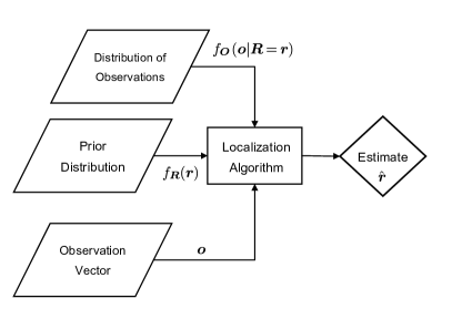
Algorithms for localization are essentially methods that derive a location estimate from the above posterior distribution. In fact, any localization algorithm $A$ is a mapping from

• the observation vector ${\bm{o}}$

• the prior distribution over the location, $f_{{\bm{R}}}({\bm{r}})$

• the conditional distribution over ${\bm{o}}$, $f_{{\bm{O}}}\left({\bm{o}}|{\bm{R}}={\bm{r}}\right)$

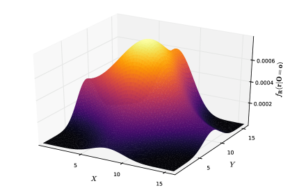
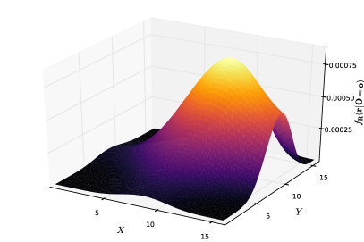
to a location estimate $\hat{{\bm{r}}}$, as illustrated in Figure 1. A visualization of the posterior distribution for the popular simple path loss model with log-normal fading is given in Figure 3.

III-A Optimization based approach to Localization

In the optimization based approach to localization that we advocate, the starting point for estimating the receiver location is a cost function that must be defined a priori. In the most general terms, the cost function is modelled as $\mathcal{C}({\bm{r}},\tilde{{\bm{r}}},{\bm{o}})$, i.e., a function of the true location ${\bm{r}}$, a given proposed location estimate $\tilde{{\bm{r}}}$, and the observation vector ${\bm{o}}$. We define the expected cost function given an observation vector as follows:

$$\operatorname*{\mathrm{E}}[\mathcal{C}({\bm{r}},\tilde{{\bm{r}}},{\bm{o}})]=\int_{{\bm{r}}\in\mathcal{S}}\mathcal{C}({\bm{r}},\tilde{{\bm{r}}},{\bm{o}})\;f_{{\bm{R}}}\left({\bm{r}}|{\bm{O}}={\bm{o}}\right)\mathrm{d}{\bm{r}}.$$ (2)

Given any cost function $\mathcal{C}$, the optimal location estimation algorithm can be obtained in a unified manner by solving the following optimization for any given observation vector to obtain the optimal estimate $\hat{{\bm{r}}}$:

$$~{}\hat{{\bm{r}}}=\operatorname*{arg\,min}_{\tilde{{\bm{r}}}}\operatorname*{\mathrm{E}}[\mathcal{C}({\bm{r}},\tilde{{\bm{r}}},{\bm{o}})].$$ (3)

Note that this optimization may be performed to obtain an arbitrarily near-optimal solution by numerically computing $\operatorname*{\mathrm{E}}[\mathcal{C}({\bm{r}},\tilde{{\bm{r}}},{\bm{o}})]$ over the discretization of a two or three dimensional search space. Given recent gains in computing power, the optimization is feasible for typical indoor localization problems. Moreover, the optimization naturally lends itself to parallel execution since the computation of the expected cost at all candidate locations are independent of each other. Assuming uniform coverage, our solution will improve on increasing the number of points in our search space. In practice, for RSS localization, these points could be spaced apart on the order of 10’s of centimeters.

Figure 2:
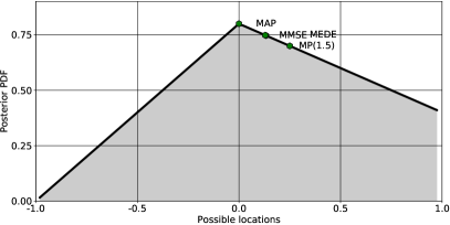
An Illustration of the distribution of true location given the observations and the locations that correspond to different optimizations. In this example, we show the different estimates returned by the various localization algorithms for a unimodal, asymmetric posterior probability density function of the form $\displaystyle f(x)=\begin{cases}\frac{4}{5}(1+x)&\quad\text{if }-1\leq x<0\\ \frac{4}{5}(1-\frac{x}{2})&\quad\text{if }0\leq x\leq 1.\\ \end{cases}$ The asymmetry of the distribution function pulls estimates other than MAP from the mode, with M$P(d)$ being the most affected. In this example, it may be shown that for $d\leq 1.5$, the M$P(d)$ estimate is $\hat{x}_{MP(d)}=\frac{d}{6}$. Thus we see that the M$P(d)$ estimate moves closer to the MAP estimate with decreasing $d$. This example serves to illustrate how differing optimization objectives can yield very different estimates for the same posterior distribution, thereby underlining the importance of deciding on an optimization objective upfront.

Existing algorithms such as MLE, MMSE, MEDE and M$P(d)$ can be recovered in our framework using suitable choices of the cost function $\mathcal{C}$. For instance, it is straightforward to verify that minimizing the expected distance error yields MEDE. Perhaps more interestingly, the MLE estimate can also be recovered using an appropriate distance based cost function. Figure 2 provides an example of how these different optimizations can yield very different location estimates.

(a)

(b)

(c)

(d)

Figure 3: Illustration of the posterior distribution of $R$ using observations taken from a log-normal distribution. For this illustration, four transmitters were placed in a $16\text{\,}\mathrm{m}$ $\times$ $16\text{\,}\mathrm{m}$ area. A log-normal path loss model was used to to determine the signal strengths. Each subplot above shows the posterior distribution of $R$ constructed by the receiver upon receiving a different vector of observations.

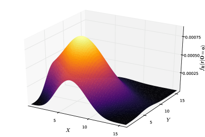
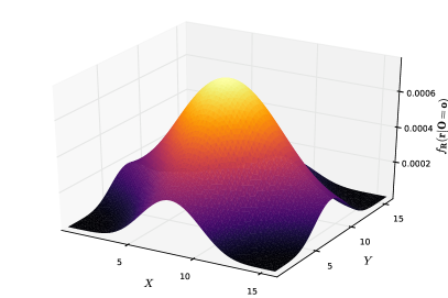
The most compelling aspect of this unified optimization-based approach to localization is its generality. Being Bayesian in nature, it can incorporate both model and data-driven approaches to characterizing the radio environment in a given space, and can accommodate prior information in a natural way (as such, it is also highly compatible with location tracking approaches that use Bayesian filtering). In addition, the framework has cognitive properties in that it gets better over time as more observations or inputs help improve the prior. While we present and evaluate our framework using RSS measurements for ease of exposition, it is not limited to such measurements. Other modalities such as ToA, TDoA [25, 26] and AoA [27] are easily incorporated as well.

IV A Unifying Framework for Evaluating Localization Algorithms

In addition to the previously defined unifying framework, we also propose the use of the distance error cdf as a unified way of evaluating localization algorithms. For a localization algorithm, say $A$, the $L_{2}$ (Euclidean) distance between the estimate ($\hat{{\bm{r}}}_{A}$) and the true location (${\bm{r}}$) is represented by the random variable $D_{A}$. Note that

$$D_{A}=\|\hat{{\bm{r}}}_{A}-{\bm{r}}\|_{2}.$$ (4)

The CDF of $D_{A}$, also termed the error cdf of algorithm $A$, may be characterized by averaging the probability that the true location lies within a certain distance, say $d$, of our estimate, over the all possible receiver locations. This notion is defined below.

Definition 1.

Let $A\in\mathcal{A}$, where $\mathcal{A}$ denotes the set of all localization algorithms. Denote by $\hat{{\bm{r}}}_{A}$ a location estimate returned by the algorithm $A$. Then, the error cdf of $A$ is a monotonically increasing function $F_{A}:\mathcal{Q}\subseteq\mathbb{R}_{\geq 0}\to[0,1]$ such that

$$F_{A}(d)=\int_{{\bm{r}}\in\mathcal{S}}P\left[D_{A}\leq d\right]f_{{\bm{R}}}({\bm{r}})\,\mathrm{d}{\bm{r}}.$$ (5)

Let $d^{*}$ be the maximum distace between any two points in $\mathcal{S}$. Then $\mathcal{Q}$ is the closed interval $[0,d^{*}]$. Using the error cdf, we may meaningfully define an ordering over the class of localization algorithms using the concept of stochastic dominance.

Definition 2.

Let $A_{1},A_{2}\in\mathcal{A}$. We say that $A_{1}$ stochastically dominates $A_{2}$ if

$$F_{A_{1}}(d)\geq F_{A_{2}}(d)\quad\forall d\in\mathcal{Q}.$$ (6)

Definition 3.

Let $A_{1},A_{2}\in\mathcal{A}$. We say that $A_{1}$ strictly stochastically dominates $A_{2}$ if in addition to equation (6), there exists $d_{1},d_{2}\in\mathcal{Q}$ such that $d_{1}<d_{2}$ and

$$F_{A_{1}}(d)>F_{A_{2}}(d)\quad\forall d\in[d_{1},d_{2}].$$ (7)

IV-A Distance Based Cost Functions

We now restrict our attention to an important class of metrics, those cost functions that can be specified to be monotonically increasing with respect to the distance between the true and estimated positions. We show that in fact localization algorithms form a partially-ordered set with respect to this important class of metrics. We also show that localization algorithms derived using the optimization-based approach for these metrics lie essentially on a “Pareto Boundary” of the set of all localization algorithms. The localization cost function, formally defined below, generalizes most metrics commonly used in the localization literature.

Definition 4.

Let $g:\mathcal{Q}\subseteq\mathbb{R}_{\geq 0}\to\mathbb{R}_{\geq 0}$ be a monotonically increasing function. Denote the set of all such functions by $\mathcal{G}$. For a localization algorithm $A$, $g(D_{A})$ is the distance error localization cost function. $\operatorname*{\mathrm{E}}\left[g(D_{A})\right]$ is the expected cost of the algorithm $A$.

We use the above notion of expected cost as a metric to compare different localization algorithms. Note that this cost function is a special case of the more general cost function introduced in the previous section. Here we are only interested in cost functions that depend on the distance between the true location and our estimate. Many localization algorithms of interest try to optimize for some distance based cost function, either explicitly or implicitly. We have seen already that MMSE, MEDE and M$P(d)$ have distance based cost functions. Although perhaps not immediately apparent, MAP may also be computed using a distance based cost function. Specifically, we may retrieve the MAP estimate using M$P(d)$ with an adequately small radius $d$ as shown in the theorem below and also borne out by our evaluation results.

Theorem 1.

If the posterior distribution $f_{{\bm{R}}|{\bm{O}}}$ is continuous and the MAP estimate lies in the interior of $\mathcal{S}$, then for any $\delta>0$ there exists $\epsilon>0$ such that,

$$\lvert P_{1}(d)-P_{2}(d)\rvert\leq\delta\quad\forall\,0<d<\epsilon,$$ (8)

where $P_{1}(d)$ and $P_{2}(d)$ give the probability of the receiver location being within distance $d$ of the MAP and the M$P(d)$ estimate respectively.

Proof.

See Appendix. ∎

IV-B Comparing Algorithms using Stochastic Dominance

In this section, we explore how we may meaningfully compare algorithms using our optimization based framework. If we are interested in a particular cost function, then comparing two algorithms is straightforward. Compute their expected cost and the algorithm with the lower cost is better. However, with stochastic dominance we can deduce something more powerful. For any two localization algorithms $A_{1}$ and $A_{2}$, if $A_{1}$ stochastically dominates $A_{2}$, then the expected cost of $A_{1}$ is lower that that of $A_{2}$ for any distance based cost function. More formally,

Theorem 2.

For any two localization algorithms $A_{1},A_{2}\in\mathcal{A}$, if $A_{1}$ stochastically dominates $A_{2}$, then

$$\operatorname*{\mathrm{E}}\left[g(D_{A_{1}})\right]\leq\operatorname*{\mathrm{E}}\left[g(D_{A_{2}})\right]\quad\forall g\in\mathcal{G}.$$ (9)

If $A_{1}$ strictly stochastically dominates $A_{2}$, then

$$\operatorname*{\mathrm{E}}\left[g(D_{A_{1}})\right]<\operatorname*{\mathrm{E}}\left[g(D_{A_{2}})\right]\quad\forall g\in\mathcal{G}.$$ (10)

Proof.

See Appendix. ∎

Theorem 2 is the first step towards ranking algorithms based on stochastic dominance. It also gives us a first glimpse of what an optimal algorithm might look like. From Theorem 2, an algorithm $A^{*}$ that stochastically dominates every other algorithm is clearly optimal for the entire set of distance based cost functions. However, it is not obvious that such an algorithm need even exist. On the other hand, we can compute algorithms that are optimal with respect to a particular cost function. As given in the following theorem, such optimality implies that the algorithm isn’t dominated by any other algorithm. In other words, if algorithm $A$ is optimal with respect to a distance based cost function $g$, then $A$ is not strictly stochastically dominated by any other algorithm $B$.

Theorem 3.

For a localization algorithm $A\in\mathcal{A}$, if there exists a distance based cost function $g\in G$ such that for any other localization algorithm $B\in\mathcal{A}$

$$\operatorname*{\mathrm{E}}\left[g\left(D_{A}\right)\right]\leq\operatorname*{\mathrm{E}}\left[g\left(D_{B}\right)\right],$$ (11)

then for all algorithms $B\in\mathcal{A}$, there exists a distance $d\in Q$ such that

$$F_{A}(d)\geq F_{B}(d).$$ (12)

Proof.

See Appendix. ∎

Theorems 2 & 3 establish the utility of ranking algorithms based on stochastic dominance. However, if we are given two algorithms, it is not necessary that one should dominate the other. As Theorem 4 shows, if they do not conform to a stochastic dominance ordering, the algorithms are incomparable.

Theorem 4.

For any two localization algorithms $A_{1}$ and $A_{2}$, if $A_{2}$ does not stochastically dominate $A_{1}$ and vice versa, then there exits distance based cost functions $g_{1},g_{2}\in\mathcal{G}$ such that

$$\operatorname*{\mathrm{E}}\left[g_{1}(D_{A_{1}})\right]<\operatorname*{\mathrm{E}}\left[g_{1}(D_{A_{2}})\right],$$ (13)

and

$$\operatorname*{\mathrm{E}}\left[g_{2}(D_{A_{2}})\right]<\operatorname*{\mathrm{E}}\left[g_{2}(D_{A_{1}})\right].$$ (14)

Proof.

See Appendix. ∎

Theorem 4 establishes the existence of a “Pareto Boundary” of the set of all localization algorithms. Choosing an algorithm from within this set depends on additional considerations such as its performance on specific cost functions of interest.

IV-C Comparison based on Upper Bound of Error CDFs

In the previous section, we focused on using stochastic dominance to rank and compare algorithms without paying much attention to what an ideal algorithm might look like. In this section, we explore this topic more detail. To begin, we ask if there exists an algorithm that dominates every other algorithm? From Theorem 2 we know that such an algorithm, if it exists, will be the best possible algorithm for the class of distance based cost functions. Moreover the error CDF of such an algorithm will be an upper bound on the error CDFs of all algorithms $A\in\mathcal{A}$.

Definition 5.

We denote the upper envelope of error CDFs for all possible algorithms $A\in\mathcal{A}$ by $F^{*}$.

We now turn our attention to formally defining the error bound $F^{*}$. Our definition also provides us with a way to compute $F^{*}$. Let $D_{A}$ represent the distance error for algorithm $A$. Consider the following class of M$P(d)$ cost functions. For each $d\in\mathcal{Q}$, let

$$~{}g_{d}\left(D\right)=\begin{cases}0&\text{if }D\leq d\\ 1&\text{if }D>d.\end{cases}$$ (15)

Then, the value of $F^{*}$ at any distance $d\in\mathcal{Q}$ may be computed using the M$P(d)$ cost function at that distance. More formally,

Definition 6.

The upper envelope of error CDFs for all possible algorithms $A\in\mathcal{A}$, $F^{*}$ is defined as

$$F^{*}(d)=\sup_{A\in\mathcal{A}}\left\{1-\operatorname*{\mathrm{E}}\left[g_{d}(D_{A})\right]\right\},\quad\forall d\in Q.$$ (16)

The upper envelope of error CDFs, $F^{*}$, satisfies the following properties:

1. $F^{*}$ stochastically dominates every algorithm $A\in\mathcal{A}$,

2. $F^{*}$ is monotonically increasing in $[0,d^{*}]$,

3. $F^{*}$ is Riemann integrable over $[0,d^{*}]$.

The monotonicity of $F^{*}$ is direct consequence of the monotonicity of CDFs. Moreover, since $F^{*}$ is monotonic, it is also Riemann integrable [28, p. 126]. In general, $F^{*}$ may not be attainable by any other algorithm. However, as we show below, it is achievable under certain circumstances, which lends credence to its claim as a useful upper bound that may be used as a basis of comparison of localization algorithms.

Given the ideal performance characteristics of $F^{*}$, it is worthwhile to investigate if it is ever attained by an algorithm. A trivial case is when the M$P(d)$ algorithm yields the same estimate for all distances of interest in the domain. In this particular case, MAP and M$P(d)$ are optimal since the error CDF of the MAP or M$P(d)$ estimate traces $F^{*}$. As an illustration consider a continuous symmetric unimodal posterior distribution over a circular space with the mode located on the center of the circle. Clearly, the MAP estimate is given by the center. Moreover, the MP$(d)$ estimate is the same at all distances, namely the center of the circle. Thus we immediately have that both the MAP and M$P(d)$ estimates have attained $F^{*}$. An extensive discussion on the attainability of $F^{*}$ can be found in Appendix F.

Thus we see that there exist conditions under which $F^{*}$ is attained by an algorithm. Consequently, it is worthwhile to search for algorithms that are close to this bound or even attain it under more general settings. This leads us directly to the second method of comparing algorithms. We identify how close the error CDFs of our algorithms get to the upper bound $F^{*}$.

Consider algorithms $A,B\in\mathcal{A}$. Intuitively, if the error CDF of $A$ is closer to $F^{*}$ than that of $B$, then it seems reasonable to expect $A$ to perform better. To make this idea precise, we need to define our measure of closeness to $F^{*}$. In the following paragraph, we propose one such measure of how close the error CDF of an algorithm $A$ is to $F^{*}$. Our proposal satisfies a nice property. Namely, searching for an algorithm that is optimal over this measure is equivalent to searching for an algorithm that minimizes a particular distance based cost function. Consequently, to specify the algorithm we only need to identify this cost function.

(a)

(b)

(c)

(d)

Figure 4: Illustration of the empirically estimated distribution of $O$ using signal strength measurements taken at different locations. Each subplot refers to the distribution of signal strength from a unique access point. The left subplots refer to measurements taken at night, while the right subplots refer to measurements taken during daytime. Our framework makes better use of the higher variance data.

Definition 7.

The area between the error CDF of algorithm $A$ and the upper envelope of error CDFs is given by

$$\Theta_{A}=\int_{0}^{d^{*}}\left(F^{*}(x)-F_{A}(x)\right)\mathrm{d}x.$$ (17)

The intuition behind our measure is can be summarized easily. We seek to find an algorithm $A$ that minimizes the “area enclosed” by $F^{*}$ and the error CDF of $A$. Note that $\Theta_{A}\geq 0$ for all $A\in\mathcal{A}$. In general, it is not clear if every measure of closeness between $F^{*}$ and $F_{A}$ will yield a cost function for us to minimize. However, if we do find such a cost function, then we have the advantage of not needing to explicit know $F^{*}$ in the execution of our algorithm. This is the case for $\Theta_{A}$ as proved in the theorem below.

Theorem 5.

The algorithm that minimizes the area between its error CDF and the upper envelope of error CDFs for all possible algorithms is the MEDE algorithm.

Proof.

See Appendix. ∎

As consequence of Theorem 5, we note that if $F^{*}$ is attainable by any localization algorithm, then it is attained by MEDE. This in turn yields a simple test for ruling out the existence of an algorithm that attains $F^{*}$. On plotting the error CDF plots of different algorithms, if we find an algorithm that is not dominated by MEDE, then we may conclude that $F^{*}$ is unattainable. Thus it is relatively easy to identify cases where there is a gap between $F^{*}$ and MEDE. However, the issue of confirming that MEDE has attained $F^{*}$ is more difficult as it involves a search over the set of all algorithms.

In summary, the utility of $F^{*}$ lies in its ability to pin point the strengths and weaknesses of a proposed algorithm. As we have seen, some algorithms such as M$P(d)$ is designed to do well at specific distances while others such as MEDE aims for satisfactory performance at all distances. Other algorithms lie somewhere in between. Consequently, choosing one algorithm over the other depends on the needs of the application utilizing the localization algorithm. Therein lies the strength of our proposed framework. It allows us to effectively reason about the applicability of an algorithm for the use case at hand.

V Evaluation

(a)

(b)

(c)

(d)

Figure 5: Comparison of error CDFs for different localization algorithms. Traditional fingerprinting based on matching the mean signal strengths is indicated by the moniker ‘FING’. Each subplot indicates the algorithm performance for a different set of test data. The left subplots refer to the case when the signal strengths are tightly clustered around the mean, while the right subplots refer to the measurements with more variance.

We evaluate the proposed framework using simulations, traces and real world experiments. In Section V-A, we provide an illustration of how fingerprinting methods fit in to the framework presented in Section III, using real-world data collected from an indoor office environment. We show that while many implementations of fingerprinting use only the mean signal strength from each transmitter, we are able to better utilize the collected data by building an empirical distribution of the received observations.

We also evaluate the performance of the MLE, M$P(d)$, MMSE and MEDE using simulations as well as using traces [7]. In both cases the signal propagation was modelled using a simplified path loss model with log-normal shadowing [23]. We also assume that the prior distribution ($f_{{\bm{R}}}$) is uniform over $\mathcal{S}$.

V-A Fingerprinting Methods

Model-based methods assume that the distribution of observations given a receiver location is known. In contrast, fingerprinting methods avoid the need to model the distribution of observations by noting that one only needs to identify the change in distribution of observations from one location to another. Most implementations simplify matters even further by assuming that mean of the observations is distinct across different locations in our space of interest. The estimated mean is thus said to ‘fingerprint’ the location.

This approach works well only in cases when the distribution of signal strengths is mostly concentrated around the mean. In this case, the approach of using only the mean signal strength amounts to approximating the signal strength distribution with a normal distribution centered at the estimated mean signal strength and variance approaching zero. However, if the distribution has significant variance this approach is likely to fail. Indeed, in the regime of significantly varying signal strengths, keeping only the mean amounts to throwing away much of the information that one has already taken pains to collect.

As already indicated in Section III, we make better use of the collected data by empirically constructing the distribution of observations $f_{{\bm{O}}}\left({\bm{o}}|{\bm{R}}={\bm{r}}\right)$. This formulation allows us to the use the same algorithms as in the model-based approach, as the only difference here is in the construction of $f_{{\bm{O}}}\left({\bm{o}}|{\bm{R}}={\bm{r}}\right)$. This is in contrast to many existing implementations where one resorts to heuristics such as clustering. Indeed, under mild assumptions it is well known that the empirical distribution converges with probability one to true distribution [29] which gives our approach the nice property that it can always do better given more data.

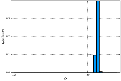
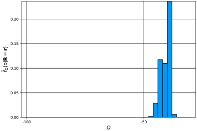
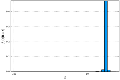
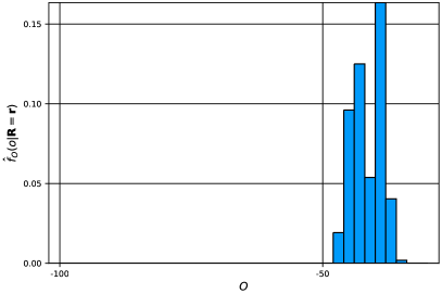
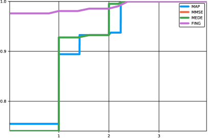
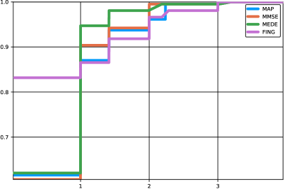
As a proof-of-concept, we compare the performance of our approach with that of traditional fingerprinting methods in two different settings. The data was collected from a $$4\text{\,}\mathrm{m}$\times$2\text{\,}\mathrm{m}$$ space inside an office environment. The space was divided into eight $$1\text{\,}\mathrm{m}$\times$1\text{\,}\mathrm{m}$$ squares and signal strength samples were collected from the center of each square. Two hundred and fifty signal strength readings were collected for the ten strongest access points detected using the WiFi card on a laptop running Linux. The beacon interval for each access point was approximately $100\text{\,}\mathrm{ms}$. The signal strength measurements were taken $400\text{\,}\mathrm{ms}$ apart. Two sets of data were collected, one at night time and the other during the day. The measurements taken at night show that the observed signal strengths are highly concentrated around the mean, as can be seen from the left subplots of Figure 4. The measurements taken during daytime show slightly more variability as can be seen in the right subplots of Figure 4.

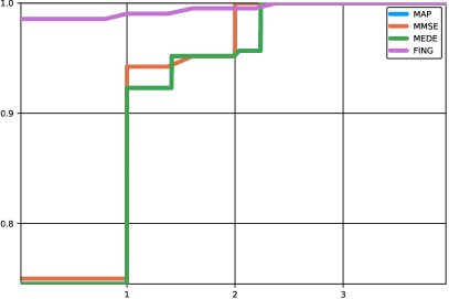
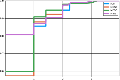
Ten percent of the collected data is randomly chosen for evaluating algorithm performance. The remaining data is used to construct the empirical distribution $\hat{f}_{{\bm{O}}}\left({\bm{o}}|{\bm{R}}={\bm{r}}\right)$ from which the MMSE, MAP and MEDE estimates are derived. It is also used to compute the mean signal strength vector or fingerprint for each location. For the algorithm denoted as ‘FING’ in Figure 5, the fingerprint closest to the test observation vector (in terms of Euclidean distance) is used to predict the location.

From the performance results given in Figure 5, we see that, as expected, the traditional fingerprinting approach works very well when the variability in the signal strength data is low. On the other hand, even with slight variability in the data, the estimates derived using our Bayesian framework outperforms traditional fingerprinting; thereby demonstrating how we may make better use of collected observation data using our framework.

V-A1 Cognitive Self-Improvement

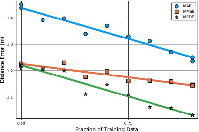
To illustrate the cognitive self-improving property of our approach, in that it performs better given more observations over time, we investigate the variation of distance error with increasing size of the training data set. The data set with more variability was chosen for the purposes of this illustration. For each fraction of the original data set, we compute the distance error for 100 random choices of the data points, for MAP, MEDE and MMSE algorithms. Figure 6 shows how the average of these distance errors varies on increasing the size of the training data set. As can be seen from Figure 6, with increasing data we are able to better estimate the empirical distribution $\hat{f}_{{\bm{O}}}\left({\bm{o}}|{\bm{R}}={\bm{r}}\right)$ from which the MMSE, MAP and MEDE estimates are derived, thereby resulting in better performance.

Figure 6: Variation of distance error with the size of the training data set. For each fraction of the original data set, we compute the distance error for 100 random choices of the data points. The regression line for each algorithm is also shown. The results indicate that our empirical estimates of the prior improves with increasing training data, which results in better algorithm performance.

V-B Simulation Model

Say $\left\{{\bm{l}}_{1},{\bm{l}}_{2},\dots,{\bm{l}}_{N}\right\}\>\left(N>2\right)$ are the known positions of $\left(N\right)$ wireless transmitters. We assume each transmitter is located on a planar surface given by $\mathcal{S}=[0,l]\times[0,b]$ where $l,b\;\in\mathbb{R}_{>{\bm{0}}}$. The locations of the transmitters are given by the two dimensional vector ${\bm{l}}_{i}=(x_{i},y_{i})\in\mathcal{S}\;\forall i\in\left\{1,2,\dots,N\right\}$. We wish to estimate the receiver locations, given by the vector ${\bm{r}}=\left(x,y\right)$, from the received signal strengths. For a given transmitter-receiver pair, say $i$, the relationship between the received signal power ($P_{r}^{i}$) and the transmitted signal power ($P_{t}^{i}$) may be modelled by the simplified path loss model:

$$P_{r}^{i}=P_{t}^{i}K{\left[\frac{d_{0}}{d_{i}}\right]}^{\eta}W_{i},$$ (18)

where the distance between the receiver and the $i^{th}$ transmitter is given by

$$d_{i}\left({\bm{r}}\right)=\sqrt{{\left(x-x_{i}\right)}^{2}+{\left(y-y_{i}\right)}^{2}},$$ (19)

and $W_{i}$ represents our noise that is log-normally distributed with zero mean and variance $\sigma^{2}$. Taking logarithm on both sides of (18), we get

$$P_{r}^{i}|_{$\mathrm{{}m}$}=P_{t}^{i}|_{$\mathrm{{}m}$}+K|_{$\mathrm{dB}$}-10\eta\log_{10}\left[\frac{d_{i}}{d_{0}}\right]+W_{i}|_{$\mathrm{dB}$},$$ (20)

where $K$ is a constant given by the gains of the receiver and transmit antennas and possibly the frequency of transmission. $d_{0}$ is a reference distance, taken to be $1$\mathrm{m}$$. In this setting, our estimation problem may be restated as follows. We are given measurements of the receiver signal strengths $\left\{P_{r}^{1},P_{r}^{2},\dots,P_{r}^{N}\right\}$ from which we are to estimate the receiver location ${\bm{r}}$. Thus, our observation vector ${\bm{O}}$ may be written as

$$O_{i} =P_{r}^{i}|_{$\mathrm{{}m}$}-P_{t}^{i}|_{$\mathrm{{}m}$}-K|_{$\mathrm{dB}$}$$ (21)

$$=W_{i}|_{$\mathrm{dB}$}-10\eta\log_{10}\left[\frac{d_{i}}{d_{0}}\right],$$ (22)

for all $i\in\{1,\dots,N\}$. In other words, the distribution of each observation is given by

$$O_{i}\sim\mathcal{N}\left(-10\eta\ln\left[d_{i}\left({\bm{r}}\right)\right],\sigma^{2}\right).$$ (23)

Finally, the distribution of the observation vector $f_{{\bm{O}}}({\bm{o}}|{\bm{R}}={\bm{r}})$ can be obtained from the above by taking the product of all the individual observation pdfs.

V-C Simulation and Trace Results

TABLE III: Normalized Performance Results

Simulations
	Likelihood	$P(\epsilon)$	$P(d)$	MSE	EDE
MLE	1.0000	0.9222	0.8994	1.4359	1.1240
M$P(\epsilon)$	0.9808	1.0000	0.9165	1.3172	1.0997
M$P(d)$	0.6963	0.7573	1.0000	1.2860	1.0857
MMSE	0.6806	0.6980	0.8737	1.0000	1.0643
MEDE	0.7247	0.7455	0.9080	1.1272	1.0000
Traces
	Likelihood	$P(\epsilon)$	$P(d)$	MSE	EDE
MLE	1.0000	0.9989	0.9865	1.1583	1.1808
M$P(\epsilon)$	0.9976	1.0000	0.9881	1.1522	1.1785
M$P(d)$	0.8213	0.8596	1.0000	1.2605	1.3760
MMSE	0.9013	0.9171	0.9797	1.0000	1.1101
MEDE	0.8529	0.8685	0.9517	1.1569	1.0000

The parameters for the simulation were chosen to be identical as that of the traces. The dimensions of the area of interest ($\mathcal{S}$) was $$50\text{\,}\mathrm{m}$\times$70\text{\,}\mathrm{m}$$. Sixteen transmitters were chosen randomly and $100$ RSSI readings were taken for each transmitter at $5$ distinct receiver locations. The transmit power was kept constant at $16\text{\,}\mathrm{{}m}$. The estimated model parameters were a path loss of $K=$39.13\text{\,}\mathrm{dB}$$ at reference distance $d_{0}=$1\text{\,}\mathrm{m}$$, fading deviation $\sigma=16.16$ and path loss exponent $\eta=3.93$. We used two distances for the M$P(d)$ algorithm: (i) $\epsilon=$0.5\text{\,}\mathrm{m}$$ was relatively small while (ii) $d=$3\text{\,}\mathrm{m}$$ covers a more sizable area. The normalized performance results are presented in Table III. Each row evaluates the performance of the indicated algorithm across different metrics, while each column demonstrates how different algorithms perform under the given metric. The performance value for each metric is normalized by the performance of the best algorithm for that metric. Thus the fact that each algorithm performs best in the metric that it is optimized for, is reflected in the occurrence of ones as the diagonal entries in the table.

As the algorithms presented here are each optimal for a specific cost function, the theory predicts that none of them are strictly stochastically dominated by any other algorithm. The results confirm this theoretical prediction. Also worthy of note is the similarity in the performance of MLE and M$P(\epsilon)$, which is in line with what we expect from Theorem 1.

Figure 7: The error CDFs of MLE, M$P(\epsilon)$, MMSE and MEDE. For this illustration, nine transmitters were placed evenly in a line and log-normal fading was assumed. Note that none of the given algorithms are strictly stochastically dominated. In addition, MLE and M$P(\epsilon)$ perform identically as expected.

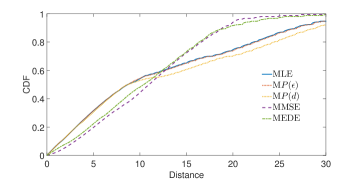
In Figure 7 we show the error CDFs of MLE, M$P(\epsilon)$, MMSE and MEDE for a linear topology. As expected, no algorithm is dominated by another and choosing $\epsilon$ to be small results in the performance of M$P(\epsilon)$ being near identical to that of MLE. Intuitively, M$P(d)$ tries to identify the region with given radius that ‘captures’ most of the a posteriori pdf $f_{{\bm{R}}}({\bm{r}}|{\bm{O}}={\bm{o}})$. Consequently for a sufficiently small radius $d$, M$P(d)$ will return a region that contains the MLE estimate. As a result, we are justified in thinking of the M$P(d)$ algorithm as a generalization of MLE (or MAP, in case our prior is non-uniform). In practice, the value of $d$ to be used will be dictated by the needs of the application that makes use of the localization service.

VI Conclusion

We have introduced an optimization based approach to localization using a general unified framework that also allows for a fair and consistent comparison of algorithms across various metrics of interest. We have demonstrated how this framework may be used to derive localization algorithms, including fingerprinting methods. We have shown the existence of a partial ordering over the set of localization algorithms using the concept of stochastic dominance, showing further that the optimality of an algorithm over a particular distance based cost function implies that the algorithm is not stochastically dominated by another. We have identified key properties of an “ideal” localization algorithm whose performance corresponds to the upper bound on error CDFs, and highlighted how we may compare different algorithms relative to this performance. Specifically, we have shown that MEDE minimizes the area between its own error CDF and the performance of such an ideal algorithm. We believe that the framework presented here goes a long way towards unifying the localization literature. The optimization based approach places the localization algorithm desideratum at the forefront, where we believe it belongs.

Appendix A Proof of Theorem 1

For ease of notation, denote the posterior distribution $f_{{\bm{R}}|{\bm{O}}}$ by $f$. Define the open ball of radius $d>0$ around ${\bm{r}}$ as

$$B_{d}({\bm{r}})=\left\{{\bm{x}}\in\mathcal{S}\mid\|{\bm{x}}-{\bm{r}}\|_{2}<d\right\}.$$ (24)

We denote the interior of $\mathcal{S}$ by ${\kern 0.0ptS}^{\mathrm{o}}$. Let ${\bm{r}}_{1}\in{\kern 0.0ptS}^{\mathrm{o}}$ be the MAP estimate. Pick any $\delta>0$. Define

$$\delta^{\prime}=\frac{\delta}{\int_{{\bm{r}}\in\mathcal{S}}\mathrm{d}{\bm{r}}}.$$ (25)

From the continuity of $f$ there exists $\epsilon>0$ such that

$$f({\bm{r}}_{1})-f({\bm{r}})<\delta^{\prime}\quad\forall\,\|{\bm{r}}_{1}-{\bm{r}}\|_{2}<\epsilon.$$ (26)

Consequently for any $0<d<\epsilon$ we have,

$$\int_{{\bm{r}}\in B_{d}({\bm{r}}_{1})}\left(f({\bm{r}}_{1})-\delta^{\prime}\right)\,\mathrm{d}{\bm{r}}\leq\int_{{\bm{r}}\in B_{d}({\bm{r}}_{1})}f({\bm{r}})\,\mathrm{d}{\bm{r}}.$$ (27)

Let ${\bm{r}}_{2}$ be the M$P(\epsilon)$ estimate. By definition,

$$\int_{{\bm{r}}\in B_{d}({\bm{r}}_{1})}f({\bm{r}})\,\mathrm{d}{\bm{r}}\leq\int_{{\bm{r}}\in B_{d}({\bm{r}}_{2})}f({\bm{r}})\,\mathrm{d}{\bm{r}}.$$ (28)

Since ${\bm{r}}_{1}$ is the MAP estimate,

$$\int_{{\bm{r}}\in B_{d}({\bm{r}}_{2})}f({\bm{r}})\,\mathrm{d}{\bm{r}}\leq\int_{{\bm{r}}\in B_{d}({\bm{r}}_{2})}f({\bm{r}}_{1})\,\mathrm{d}{\bm{r}}.$$ (29)

Combining the above inequalities together, we conclude

$$(f({\bm{r}}_{1})-\delta^{\prime})\int_{{\bm{r}}\in B_{d}({\bm{r}}_{1})}\mathrm{d}{\bm{r}} \leq P_{1}(d)\leq P_{2}(d)\leq f({\bm{r}}_{1})\int_{{\bm{r}}\in B_{d}({\bm{r}}_{2})}\mathrm{d}{\bm{r}}.$$ (30)

Note that the difference between the upper and lower bounds in the above inequality is at most $\delta$. Consequently, the difference $\lvert P_{1}(d)-P_{2}(d)\rvert$ is also bounded by $\delta$,

$$\lvert P_{1}(d)-P_{2}(d)\rvert\leq\delta\quad\forall\,0<d<\epsilon.$$ (31)

∎

Appendix B Proof of Theorem 2

Recall that the domain of the cost function is given by $\mathcal{Q}\subseteq\mathbb{R}_{\geq 0}$. For any element $p$ in the range of the cost function, the inverse image of $p$ is given by

$$g^{-1}(p)=\left\{d\in\mathcal{Q}\mid g(d)=p\right\}.$$ (32)

Let $h(p)=\inf\left(g^{-1}(p)\right)$. From the monotonicity of $g(d)$, we conclude that $h(p)$ is monotonically increasing in $p$. Moreover, we have the following relation for any algorithm $A\in\mathcal{A}$

$$P\left(g(D_{A})\leq p\right)=P\left(D_{A}\leq h(p)\right).$$ (33)

This allows us to characterize the CDF of $g(D_{A})$ as $F_{A}\left(h\left(g(d_{A})\right)\right)$. Moreover, since cost functions are non-negative, $g(D_{A})\geq 0$. Thus the expected value of $g(D_{A})$ for any algorithm $A$ may be expressed as

$$\operatorname*{\mathrm{E}}\left[g(D_{A})\right]=\int_{0}^{\sup(\mathcal{Q})}\left(1-F_{A}\left(h\left(g(d_{A})\right)\right)\right)\,\mathrm{d}d_{A}.$$ (34)

Consider any two algorithms $A_{1}$ and $A_{2}$ such that $A_{1}$ stochastically dominates $A_{2}$. From (6), we have

$$F_{A_{1}}\left(h\left(g(d)\right)\right)\geq F_{A_{2}}\left(h\left(g(d)\right)\right)\quad\forall d\in\mathcal{Q}.$$ (35)

From (34) and (35), we conclude

$$\operatorname*{\mathrm{E}}\left[g(D_{A_{1}})\right]\leq\operatorname*{\mathrm{E}}\left[g(D_{A_{2}})\right],$$ (36)

which proves (9). If $A_{1}$ strictly dominates $A_{2}$, then in addition to (35), $A_{1}$ and $A_{2}$ satisfies

$$F_{A_{1}}\left(h\left(g(d)\right)\right)>F_{A_{2}}\left(h\left(g(d)\right)\right)\quad\forall d\in[d_{1},d_{2}].$$ (37)

From (34), (35) and (37) we have

$$\operatorname*{\mathrm{E}}\left[g(D_{A_{1}})\right]<\operatorname*{\mathrm{E}}\left[g(D_{A_{2}})\right].$$ (38)

∎

Appendix C Proof of Theorem 3

Say $A\in\mathcal{A}$ is the optimal algorithm for the distance based cost function $g\in\mathcal{G}$. Further assume that for some algorithm $B\in\mathcal{A}$,

$$F_{A}(d)\leq F_{B}(d)\quad\forall d\in\mathcal{Q},$$ (39)

and that there exists some $d^{\prime}\in\mathcal{Q}$ such that $F_{A}(d^{\prime})<F_{B}(d^{\prime})$. If these conditions implied that $A$ is strictly dominated by $B$, then by Theorem 2 we have

$$\operatorname*{\mathrm{E}}\left[g(D_{A})\right]>\operatorname*{\mathrm{E}}\left[g(D_{B})\right].$$ (40)

However, from the optimality of $A$ with respect to $g$,

$$\operatorname*{\mathrm{E}}\left[g(D_{A})\right]\leq\operatorname*{\mathrm{E}}\left[g(D_{B})\right],$$ (41)

which contradicts (40). To complete the proof of Theorem 3 we need to show the strict dominance of $B$ over $A$. Since the error CDFs are right continuous, for any $\epsilon>0$ there exists a $\delta>0$ such that

$$F_{B}(d)-F_{B}(d^{\prime}) <\epsilon\quad\forall d\in[d^{\prime},d^{\prime}+\delta],$$ (42)

and

$$F_{A}(d)-F_{A}(d^{\prime}) <\epsilon\quad\forall d\in[d^{\prime},d^{\prime}+\delta].$$ (43)

Choosing $\epsilon<\frac{F_{B}(d^{\prime})-F_{A}(d^{\prime})}{2}$ implies

$$F_{B}(d)>F_{A}(d)\quad\forall d\in[d^{\prime},d^{\prime}+\delta],$$ (44)

which proves that $B$ strictly dominates $A$. ∎

Appendix D Proof of Theorem 4

Since $A_{2}$ does not stochastically dominate $A_{1}$, there exists some $d_{1}\in\mathcal{Q}$ such that

$$F_{A_{1}}\left(d_{1}\right)>F_{A_{2}}\left(d_{1}\right).$$ (45)

Since $A_{1}$ does not stochastically dominate $A_{2}$, there exists some $d_{2}\in\mathcal{Q}$ such that

$$F_{A_{1}}\left(d_{2}\right)<F_{A_{2}}\left(d_{2}\right).$$ (46)

Define the cost functions $g_{1}$ and $g_{2}$ as

$$g_{1}\left(D\right)=\begin{cases}0&\text{if }D\leq d_{1}\\ 1&\text{if }D>d_{1},\end{cases}$$ (47)

and

$$g_{2}\left(D\right)=\begin{cases}0&\text{if }D\leq d_{2}\\ 1&\text{if }D>d_{2}.\end{cases}$$ (48)

Thus,

$$\operatorname*{\mathrm{E}}\left[g_{1}(D_{A_{1}})\right] =1-F_{A_{1}}(d_{1})$$ (49)

$$<1-F_{A_{2}}(d_{1})=\operatorname*{\mathrm{E}}\left[g_{1}(D_{A_{2}})\right],$$ (50)

where the inequality follows from (45). Similarly,

$$\operatorname*{\mathrm{E}}\left[g_{2}(D_{A_{2}})\right] =1-F_{A_{2}}(d_{2})$$ (51)

$$<1-F_{A_{1}}(d_{2})=\operatorname*{\mathrm{E}}\left[g_{2}(D_{A_{1}})\right],$$ (52)

where the inequality in the second step follows from (46). ∎

Appendix E Proof of Theorem 5

As $F^{*}$ dominates every other algorithm, the area under the CDF curve of any other algorithm is no greater than the area under $F^{*}$. Consequently, maximizing $R_{A}$ is equivalent to maximizing the area under the CDF curve of the algorithm. We use this fact to show that the expected distance error of algorithm $A$, $\operatorname*{\mathrm{E}}\left[D_{A}\right]$ is a linear function of $R_{A}$. Thus an algorithm that minimizes $R_{A}$ minimizes $\operatorname*{\mathrm{E}}\left[D_{A}\right]$ as well and vice versa. More formally, for all $A\in\mathcal{A}$

$$R_{A} =\int_{0}^{d^{*}}\left(F^{*}(x)-F_{A}(x)\right)\mathrm{d}x$$ (53)

$$=\int_{0}^{d^{*}}\left(1-F_{A}(x)\right)\mathrm{d}x+\int_{0}^{d^{*}}\left(F^{*}(x)-1\right)\mathrm{d}x$$ (54)

$$=\operatorname*{\mathrm{E}}\left[D_{A}\right]+\alpha,$$ (55)

where the last equality follows from the fact that the random variable $D_{A}$ is non-negative and $\alpha$ is the constant given by $\alpha=\int_{0}^{d^{*}}\left(F^{*}(x)-1\right)\mathrm{d}x$. ∎

Appendix F Attainability of the optimal error CDF

As indicated in Section IV-C, if we have a symmetric unimodal distribution over a circular area with the mode located at the center, then the MAP estimate is optimal. On the other hand, from an algorithmic perspective, MEDE has the nice property, following Theorem 3, that if there exists an algorithm that attains $F^{*}$, then the MEDE algorithm will attain it as well. However, it is not clear a priori if $F^{*}$ is attainable. A sufficient and necessary condition for the attainability $F^{*}$ may be obtained in light of the following observations:

• By design, the M$P(d)$ estimate matches the performance of $F^{*}$ for the specific distance $d\in\mathcal{Q}$. However, there are no guarantees on the performance the estimate at other distances.

• The M$P(d)$ algorithm need not return a unique location estimate. This reflects the fact that there may be multiple locations in $\mathcal{S}$ that maximizes the $P(d)$ metric for the given posterior distribution.

Consequently, consider a modified version of the M$P(d)$ algorithm that enumerates all possible M$P(d)$ estimates for the given distance $d$. If $F^{*}$ is attainable by some algorithm $A$, then the estimate returned by $A$, say $\hat{{\bm{r}}}_{A}$, must exist in the list returned by the M$P(d)$ algorithm. Note that this condition holds for any distance $d\in\mathcal{Q}$ used for the M$P(d)$ algorithm. Consequently, if the intersection of the estimate list returned by M$P(d)$ for all $d\in\mathcal{Q}$ is non-empty, then we conclude that $F^{*}$ is attained by each estimate in the intersection. If the intersection is a null set, then we conclude that $F^{*}$ is unattainable, thereby giving us the necessary and sufficient condition for the existence of $F^{*}$.

While the above test calls for the repeated execution of the M$P(d)$ algorithm over a potentially large search space, we may exploit the fact that each execution is independent of each other, thereby gaining considerable speed improvements by utilizing parallel processing. In some cases, it may be possible to carry out this test analytically. The condition enumerated in Section IV-C is a case in point. The task of identifying the cases when we can obtain the algorithm that attains $F^{*}$ is a topic of future research. A slight generalization of the example given in Section IV-C leads to the following conjecture.

Conjecture 1.

If the posterior distribution $f_{{\bm{R}}}({\bm{r}}|{\bm{O}}={\bm{o}})$ is continuous, symmetric and unimodal with the mode located at the centroid of a convex space $\mathcal{S}$, then the MAP estimate is optimal.

Let $d^{\prime}$ be the maximal radius of a neighbourhood $N_{d}({\bm{c}})\subseteq\mathcal{S}$ centered on the centroid (${\bm{c}}$) of our space $\mathcal{S}$. For all $d\leq d^{\prime}$

$$\inf_{{\bm{r}}\in N_{d}({\bm{c}})}f_{{\bm{R}}}({\bm{r}}|{\bm{O}}={\bm{o}})\geq\sup_{{\bm{r}}\in N_{d}({\bm{r}}^{\prime})\setminus N_{d}({\bm{c}})}f_{{\bm{R}}}({\bm{r}}|{\bm{O}}={\bm{o}}),$$ (56)

for any ${\bm{r}}^{\prime}\in\mathcal{S}$. Note that this follows directly from the assumption that the posterior is unimodal. Consequently, for all $d\leq d^{\prime}$ the MAP estimate is one of the best performing estimates. The optimality of MAP at distances beyond $d^{\prime}$ follows immediately if

$$\int_{\mathcal{S}\cap(N_{d}({\bm{c}})\setminus N_{d}({\bm{r}}^{\prime}))}\mathrm{d}{\bm{r}}\geq\int_{\mathcal{S}\cap(N_{d}({\bm{r}}^{\prime})\setminus N_{d}({\bm{c}}))}\mathrm{d}{\bm{r}},$$ (57)

for any ${\bm{r}}^{\prime}\in\mathcal{S}$. We intuit that the above condition holds since ${\bm{c}}$ is the centroid of $\mathcal{S}$, but a proof remains elusive.

References

- [1] A. Waadt, C. Kocks, S. Wang, G. Bruck, and P. Jung, “Maximum likelihood localization estimation based on received signal strength,” in Proc. IEEE ISABEL’10, Nov. 2010, pp. 1–5.
- [2] Y.-F. Huang, Y.-T. Jheng, and H.-C. Chen, “Performance of an MMSE based indoor localization with wireless sensor networks,” in Proc. IEEE NCM’10, Aug. 2010, pp. 671–675.
- [3] L. Lin and H. So, “Best linear unbiased estimator algorithm for received signal strength based localization,” in Proc. IEEE EUSIPCO’11, Aug. 2011, pp. 1989–1993.
- [4] P. Bahl and V. Padmanabhan, “RADAR: an in-building RF-based user location and tracking system,” in Proc. IEEE INFOCOM’00, vol. 2, Mar. 2000, pp. 775–784.
- [5] K. Yedavalli and B. Krishnamachari, “Sequence-based localization in wireless sensor networks,” IEEE Trans. Mobile Comput., vol. 7, no. 1, pp. 81–94, Jan. 2008.
- [6] D. Fox, J. Hightower, L. Liao, D. Schulz, and G. Borriello, “Bayesian filtering for location estimation,” IEEE Pervasive Comput., vol. 2, no. 3, pp. 24–33, Jul. 2003.
- [7] K. Bauer, E. W. Anderson, D. McCoy, D. Grunwald, and D. C. Sicker, “CRAWDAD data set cu/rssi (v. 2009-05-28),” Downloaded from http://crawdad.org/cu/rssi/, May 2009.
- [8] M. Youssef, A. Agrawala, and A. Udaya Shankar, “WLAN location determination via clustering and probability distributions,” in Proc. IEEE PerCom’03, Mar. 2003, pp. 143–150.
- [9] G. Zanca, F. Zorzi, A. Zanella, and M. Zorzi, “Experimental comparison of RSSI-based localization algorithms for indoor wireless sensor networks,” in Proc. ACM RealWSN’08, 2008, pp. 1–5.
- [10] V. Seshadri, G. Zaruba, and M. Huber, “A bayesian sampling approach to in-door localization of wireless devices using received signal strength indication,” in Proc. IEEE PerCom’05, Mar. 2005, pp. 75–84.
- [11] M. Youssef and A. Agrawala, “The horus wlan location determination system,” in Proc. ACM MobiSys’05, 2005, pp. 205–218.
- [12] Z. Yang, C. Wu, and Y. Liu, “Locating in fingerprint space: Wireless indoor localization with little human intervention,” in Proc. ACM MobiCom’12, 2012, pp. 269–280.
- [13] J. Blumenthal, R. Grossmann, F. Golatowski, and D. Timmermann, “Weighted centroid localization in zigbee-based sensor networks,” in Proc. IEEE WISP’07, Oct. 2007, pp. 1–6.
- [14] N. Patwari, A. Hero, M. Perkins, N. Correal, and R. O’Dea, “Relative location estimation in wireless sensor networks,” IEEE Trans. Signal Process., vol. 51, no. 8, pp. 2137–2148, Aug. 2003.
- [15] S. Chitte, S. Dasgupta, and Z. Ding, “Distance estimation from received signal strength under log-normal shadowing: Bias and variance,” IEEE Signal Process. Lett., vol. 16, no. 3, pp. 216–218, Mar. 2009.
- [16] H. Aksu, D. Aksoy, and I. Korpeoglu, “A study of localization metrics: Evaluation of position errors in wireless sensor networks,” Comput. Netw., vol. 55, no. 15, pp. 3562–3577, Oct. 2011.
- [17] E. Elnahrawy, X. Li, and R. Martin, “The limits of localization using signal strength: a comparative study,” in Proc. IEEE SECON’04, Oct. 2004, pp. 406–414.
- [18] S. H. Low and D. E. Lapsley, “Optimization flow control i: Basic algorithm and convergence,” IEEE/ACM Trans. Netw., vol. 7, no. 6, pp. 861–874, Dec. 1999.
- [19] S. Shakkottai and R. Srikant, Network Optimization and Control, in Foundations and Trends in Networking. Boston - Delft: Now Publishers Inc, Jan. 2008.
- [20] B. Shahriari, K. Swersky, Z. Wang, R. P. Adams, and N. de Freitas, “Taking the human out of the loop: A review of bayesian optimization,” Proceedings of the IEEE, vol. 104, no. 1, pp. 148–175, Jan 2016.
- [21] J. Jacob, B. R. Jose, and J. Mathew, “Spectrum prediction in cognitive radio networks: A bayesian approach,” in 2014 Eighth International Conference on Next Generation Mobile Apps, Services and Technologies, Sept 2014, pp. 203–208.
- [22] X. Xing, T. Jing, Y. Huo, H. Li, and X. Cheng, “Channel quality prediction based on bayesian inference in cognitive radio networks,” in 2013 Proceedings IEEE INFOCOM, April 2013, pp. 1465–1473.
- [23] A. F. Molisch, Wireless Communications, 2nd ed. Chichester, West Sussex, U.K: Wiley, 2010.
- [24] N. A. Jagadeesan. (2017) Lczn.jl. [Online]. Available: https://github.com/ANRGUSC/Lczn.jl
- [25] N. B. Priyantha, A. Chakraborty, and H. Balakrishnan, “The cricket location-support system,” in Proc. ACM MobiCom’00, 2000, pp. 32–43.
- [26] A. Savvides, C.-C. Han, and M. B. Strivastava, “Dynamic fine-grained localization in ad-hoc networks of sensors,” in Proc. ACM MobiCom’01, 2001, pp. 166–179.
- [27] D. Niculescu and B. Nath, “Ad hoc positioning system (APS) using AoA,” in Proc. IEEE INFOCOM’03, vol. 3, Mar. 2003, pp. 1734–1743.
- [28] W. Rudin, Principles of Mathematical Analysis, 3rd ed. New York: McGraw-Hill Science/Engineering/Math, Jan. 1976.
- [29] H. G. Tucker, “A generalization of the glivenko-cantelli theorem,” Ann. Math. Statist., vol. 30, no. 3, pp. 828–830, 09 1959. [Online]. Available: http://dx.doi.org/10.1214/aoms/1177706212