Customer Lifetime Value Prediction Using Embeddings

Abstract.

We describe the Customer LifeTime Value (CLTV) prediction system deployed at ASOS.com, a global online fashion retailer. CLTV prediction is an important problem in e-commerce where an accurate estimate of future value allows retailers to effectively allocate marketing spend, identify and nurture high value customers and mitigate exposure to losses. The system at ASOS provides daily estimates of the future value of every customer and is one of the cornerstones of the personalised shopping experience. The state of the art in this domain uses large numbers of handcrafted features and ensemble regressors to forecast value, predict churn and evaluate customer loyalty. Recently, domains including language, vision and speech have shown dramatic advances by replacing handcrafted features with features that are learned automatically from data. We detail the system deployed at ASOS and show that learning feature representations is a promising extension to the state of the art in CLTV modelling. We propose a novel way to generate embeddings of customers, which addresses the issue of the ever changing product catalogue and obtain a significant improvement over an exhaustive set of handcrafted features.

1. Introduction

ASOS is a global e-commerce company, based in the UK and specialising in fashion and beauty. The business is entirely online, and products are sold through eight country-specific websites and mobile apps. At the time of writing, there were 12.5 million active customers and the product catalogue contained more than 85,000 items. Products are shipped to 240 countries and territories and the annual revenue for 2016 was £1.4B, making ASOS one of Europe’s largest pure play online retailers.

An integral element of the business model at ASOS is free delivery and returns. Free shipping is vital in online clothing retail because customers need to try on items without being charged. Since ASOS do not recoup delivery costs for returned items, customers can easily have negative lifetime value. For this reason the Customer LifeTime Value (CLTV) problem is particularly important in online clothing retail.

Our CTLV system addresses two tightly coupled problems: CLTV and churn prediction. We define a customer as churned if they have not placed an order in the past year. We define CLTV as the sales, net of returns, of a customer over a one year period. The objective is to improve three key business metrics: (1) the average customer shopping frequency, (2) the average order size, (3) the customer churn rate. The model supports the first two objectives by allowing ASOS to rapidly identify and nurture high-value customers, who will go on to have high frequency, high-order size, or both. The third objective is achieved by identifying customers at high risk of churn and controlling the amount spent on retention activities.

State-of-the-art CLTV systems use large numbers of handcrafted features and ensemble classifiers (typical random forest regressors), which have been shown to perform well in highly stochastic problems of this kind (Vanderveld et al., 2016; Hardie et al., 2006). However, handcrafted features introduce a human bottleneck, can be difficult to maintain and often fail to utilise the full richness of the data. We show how automatically learned features can be combined with handcrafted features to produce a model that is both aware of domain knowledge and can learn rich patterns of customer behaviour from raw data.

The deployed ASOS CLTV system uses the state-of-the-art architecture, which is a Random Forest (RF) regression model with 132 handcrafted features. To train the forest, labels and features are taken from disjoint periods of time as shown in the top row of Figure 1. The labels are the net spend (sales minus returns) of each customer over the past year. The training labels and features are used to learn the parameters of the RF. The second row of Figure 1 shows the live system where the RF parameters from the training period are applied to new features generated from the last year’s data to produce prediction for net customer spend over the next year.

Figure 1. Training and prediction time-scales for CLTV. The model is retrained every day using customer data from the past two years. Labels are the net customer spend over the previous year. Model parameters are learned in the training period and used to predict CLTV from new features in the live system.

We provide a detailed explanation of the challenges and lessons learned in deploying the ASOS CLTV system and describe our latest efforts to improve this system by augmenting it with learned features. Our approach is inspired by the recent successes of representation learning in the domains of vision, speech and language. We experimented with learning representations directly from data using two different approaches: (1) by training a feedforward neural network on the handcrafted features in a supervised setting (see Section 4.2); (2) By augmenting the RF feature set with unsupervised customer embeddings learnt from web and app browsing data (see Section 4.1). The novel customer embeddings are shown to improve CLTV prediction performance significantly compared with our benchmark. Incorporating embeddings into long-term prediction models is challenging because, unlike handcrafted features, the features are not easily identifiable. Figure 2 illustrates this point using a four dimensional embedding. Each column in the figure corresponds to a different dimension of the embeddings space and also a feature of the random forest model. In the training period we learn parameters for each feature. However, as the features are not labelled and their order randomly permutes from training to test time, it is not possible to map the training parameters to the test features. We describe how this problem can be solved within the neural embedding framework using a form of warm start for the test period embeddings.

Figure 2. Illustration of the challenges of using the components of embedded customer vectors as features for forecasting. Each column represents a component of the vector representation of customers. We have labelled the columns with the parameters that are learnt at training time. (Left) The vector components randomly permute between train and testing time and hence require different learned parameters. (Right) Applying the learned parameters from training time directly to the embeddings in test time will not work as they are no longer attached to the correct component of the embedded vectors.

Therefore, our main contributions are:

1. A detailed description of the large-scale CLTV system deployed at ASOS, including a discussion of the architecture, deployment challenges and lessons learned.

2. Analysis of two candidate architectures for hybrid systems that incorporate both handcrafted and learned features

3. Introduction of customer level embeddings and demonstration that these produce a significantly better performance than a benchmark classifier

4. We show how to use neural embeddings for long-term prediction tasks

2. Related Work

Statistical models of customer purchasing behaviour have been studied for decades. Early models were hampered by a lack of data and were often restricted to fitting simple parametric statistical models, such as the Negative Binomial Distribution in the NBD model (Morrison et al., 1988). It was only at the turn of the century, with the advent of large-scale e-commerce platforms that this problem began to attract the attention of machine learning researchers.

2.1. Distribution Fitting Approaches

The first statistical models of CLTV were known as “Buy ’Til You Die” (BTYD) models. BTYD models place separate parametric distributions on the customer lifetime and the purchase frequency and only require customer recency and frequency as inputs. One of the first models was the Pareto/NBD model (Schmittlein et al., 1987), which assumes an exponentially distributed active duration and a Poisson distributed purchase frequency for each customer. This yields a Pareto-II customer lifetime and negative-binomial (NBD) distributed purchase frequency. Fader et al. (Fader et al., 2005a) replaced the Pareto-II with a Beta-geometric distribution for easier implementation, assuming each customer has a certain probability to become inactive after every purchase. Bemmaor et al. (Bemmaor and Glady, 2012) proposed the Gamma/Gompertz distribution to model the customer active duration, which is more flexible than the Pareto-II as it can have a non-zero mode and be skewed in both directions.

Recency-Frequency-Monetary Value (RFM) models expand on BTYD by including an additional feature. Fader et al. (Fader et al., 2005b) linked the RFM model, which captures the time of last purchase (recency), number of purchases (frequency) and purchase values (monetary value) of each customer to CLTV estimation. Their model assumes a Pareto/NBD model for recency and frequency with purchase values following an independent gamma/gamma distribution.

While successful for the problems that they were applied to, it is difficult to incorporate the vast majority of the customer data available to modern e-commerce companies into the RFM/BYTD framework. It is particularly difficult to incorporate automatically learned or highly sparse features. This motivates the need for machine learning approaches to the problem.

2.2. Machine Learning Methods

The most related work to ours is that of Vanderveld et al. (2016), which is the first work to explicitly include customer engagement features in a CLTV prediction model. They also address the challenges of learning the complex, non-linear CLTV distribution by solving several simpler sub-problems. Firstly, a binary classifier is run to identify customers with predicted CLTV greater than zero. Secondly, the customers predicted to shop again are split into five groups and independent regressors are trained for each group. To the best of our knowledge, deep neural networks have not yet been successfully applied to the CLTV problem. However, there is work on the related churn problem (CLTV greater than zero) by Wangperawong et al. (2016) for telecommunications. The authors create a two-dimensional array for each customer where the columns are days of the year and the rows describe different kinds of communication (text, call etc.). They used this array to train deep convolutional neural networks. The model also used auto-encoders (Vincent et al., 2008) to learn low-dimensional representations of the customer arrays.

2.3. Neural Embeddings

Neural embeddings are a technique pioneered in Natural Language Processing (NLP) for learning distributed representations of words (Mikolov et al., 2013). They provide an alternative to the one-of-$k$ (or one-hot) representation. Unlike the one-of-$k$ representation, which uses large sparse orthogonal vectors (which are equally similar), embeddings are compact, dense representations that encapsulate similarity. Embedded representations have been shown to give superior performance to sparse representations in several downstream tasks in language and graph analysis (Perozzi and Skiena, 2014; Mikolov et al., 2013). All embedding methods define a context that groups objects. Typically, the data is a sequence and the context is a fixed-length window that is passed along the sequence. The model learns that objects frequently occurring in the same context are similar and will have embeddings with high cosine similarity.

One of the most popular embedding models is SkipGram with Negative Sampling (SGNS), which was developed by Mikolov et al. (2013). It has found a broad range of applications and we describe the most relevant to our work. Barkan and Koenigstein (2016) used SGNS for item-level embeddings in item-based collaborative filtering, which they called item2vec. As a context the authors use a basket of items that were purchased together . In (Grbovic et al., 2015) SGNS was used to generate a set of product embeddings, which the authors called prod2vec, by mining receipts from email data. For each customer a sequence of products was built (with arbitrary ordering for those bought together) and then a context window was run over it. The goal was to predict products that are co-purchased by a single customer within a given number of purchases. The authors also proposed a hierarchical extension called bagged-prod2vec that groups products appearing together in a single email. (Baeza-yates et al., 2015) used a variant of SGNS to predict the next app a mobile phone user would open. The key idea is to consider sequences of app usage within mobile sessions. The data had associated time stamps, which the authors used to modify the original model. Instead of including every pairwise set of apps within the context, the selection probability was controlled by a Gaussian sampling scheme based on the inter-open duration.

3. Customer Lifetime Value Model

The ASOS CLTV model uses a rich set of features to predict the net spend of customers over the next 12 months by training a random forest regressor on historic data. One of the major challenges of predicting CLTV is the unusual distribution of the target variable. A large percentage of customers have a CLTV of zero. Of the customers with greater than zero CLTV, the values differ by several orders of magnitude. To manage this problem we explicitly model CLTV percentiles using a random forest regressor. Having predicted percentiles, the outputs are then mapped back to real value ranges for use in downstream tasks.

The remainder of this section describes the features used by the model, the architecture that allows the model to scale to over 10 million customers, and our training and evaluation methodology.

3.1. Features

The model incorporates features from the full spectrum of customer information available at ASOS. There are four broad classes of data: (1) customer demographics, (2) purchase history (3) returns history (4) web and app session logs. By far the largest and richest of these classes are the session logs.

We apply random forest feature importance (Friedman et al., 2001) to rank the 132 handcrafted features. Table 1 shows the feature importance breakdown by the broad classes of data and Table 2 shows the top features. As expected, the number of orders, the number of sessions in the last quarter and the nationality of the customer were very important features for CLTV prediction. However, we were surprised by the importance of the standard deviation of the order and session dates, particularly because the maximum spans of these variables were also features. We also did not expect the number of items purchased from the new collection to be one of the most relevant features. This is because newness is a major consideration for high value fashion customers.

Table 1. Feature importance by data class.

Data class	Overall Importance
Customer demographics	0.078
Purchases history	0.600
Returns history	0.017
Web/app session logs	0.345

Table 2. Individual feature importance (top features).

Feature Name	Importance
Number of orders	0.206
Standard deviation of the order dates	0.115
Number of session in the last quarter	0.114
Country	0.064
Number of items from new collection	0.055
Number of items kept	0.049
Net sales	0.039
Days between first and last session	0.039
Number of sessions	0.035
Customer tenure	0.033
Total number of items ordered	0.025
Days since last order	0.021
Days since last session	0.019
Standard deviation of the session dates	0.018
Orders in last quarter	0.016
Age	0.014
Average date of order	0.009
Total ordered value	0.008
Number of products viewed	0.007
Days since first order in last year	0.006
Average session date	0.006
Number of sessions in previous quarter	0.005

3.2. Architecture

Figure 3. High-level overview of the CLTV system. The solid arrows represent the flow of data, and the dashed arrows represents interaction between stakeholders and systems/data. Customer data is collected and pre-processed by our data warehouse and stored on Microsoft Azure blob storage. The processed data is used to generate handcrafted features in Spark clusters, with web/app sessions additionally used to produce experimental customer embeddings in Tensorflow. The handcrafted features and customer embeddings are then fed through the machine learning pipeline on Spark, which trains calibrated random forests for churn classification and CLTV regression. The resulting prediction are piped to operational systems.

The high-level system architecture is shown in Figure 3. Raw customer data (see Section 3.1) is pre-processed in our data warehouse and stored in Microsoft Azure blob storage. From blob storage, data flows through two work streams to generate customer features: A handcrafted feature generator on Apache Spark and an experimental customer embedding generator on GPU machines running Tensorflow(Abadi et al., 2015), which uses only the web/app sessions as input. The model is trained in two stages using an Apache Spark ML pipeline. The first stage pre-processes the features and trains random forests for churn classification and CLTV regression on percentiles. The second stage performs calibration and maps percentiles to real values. Finally the predictions are presented to a range of business systems that trigger personalised engagement strategies with ASOS customers.

3.3. Training and Evaluation Process

Our live system uses a calibrated random forest model with features from the past twelve months that is re-trained every day. We use twelve months because there are strong seasonality effects in retail and failing to use an exact number of years would cause fluctuations in features that are calculated by aggregating data over the training period.

To train the model we use historic net sales over the last year as a proxy for CLTV labels and learn the random forest parameters using features generated from a disjoint period prior to the label period. This is illustrated in Figure 1. Every day we generate:

1. A set of aggregate features and product view-based embeddings for each customer based on their demographics, purchases, returns and web/app sessions between two years and one year ago,

2. Corresponding target labels, including the churn status and net one-year spend, for each customer based on data from the last year.

The feature and label periods are disjoint to prevent information leakage. As the predictive accuracy of our live system could only be evaluated in a year’s time, we establish our expectation on the performance of the model by forecasting for points in the past for which we already know the actual values as illustrated in Figure 1. We use the Area Under the receiver operating characteristic Curve (AUC) as a performance measure.

3.4. Calibration

In this context, calibration refers to our efforts to ensure that the statistics of the model predictions are consistent with the statistics of the data. Model predictions are derived from RF leaf distributions and we perform calibration for both churn and CLTV prediction.

For customer churn prediction, choosing RF classifier parameters that maximise the AUC does not guarantee that the predictive probabilities will be consistent with the realised churn rate (Zadrozny and Elkan, 2001). To generate consistent probabilities, we calibrate by learning a mapping between the estimates and the realised probabilities. This is done by training a one-dimensional logistic regression classifier to predict churn based only on the probabilities returned by the random forest. The logistic regression output is interpreted as a calibrated probability. Similarly, to estimate CLTV we have no guarantees that the regression estimates achieved by minimizing the Root Mean Squared Error (RMSE) loss function will match the realised CLTV distribution. To address this problem, analogously to churn probability calibration, we first forecast the CLTV percentile and then map the predicted percentiles into monetary values. In this case, the mapping is learnt using a decision tree. We observe two advantages in performing calibration: (1) the model becomes more robust to the existence of outliers and (2) we obtain predictions, which when aggregated over a set of customers, match the true values more accurately.

3.5. Results

To find the optimal meta-parameters for the RFs we use 10-fold cross validation on a sample of the data. For CLTV predictions (see Figure 4) we obtain Spearman rank-order correlation coefficients of 0.56 (for all customers) and 0.46 (excluding customers with a CLTV of 0). We can see in Figure 4 that the range and density of the predicted CLTV matches the actual CLTV (excluding customers with an LTV of 0). For the churn predictions (see Figure 5) we obtain an AUC of 0.798 and calibrated probabilities.

Figure 4. Predicted CLTV against actual CLTV (excluding customers with an actual CLTV of 0). Units (horizontal and vertical axis) are the average CLTV value in GBP. The distribution of the prediction and the actual CLTV are similar in log scale (top and right density plots). The central plot shows the fit between the predictions and the actual values, which have a Spearman rank-order correlation coefficient of 0.46.

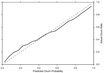
Figure 5. Churn prediction density (horizontal axis) and match between predicted probabilities and actual probabilities (black line) versus the optimal calibration (dashed grey line). The predicted probabilities match closely with the actual probabilities

.

4. Improving the CLTV model with feature learning

In the remainder of the paper we describe our ongoing efforts to supplement the handcrafted features in our deployed system with automatic feature learning. Feature learning is the process of learning features directly from data, so as to maximise the objective function of the classification or regression task. This technique is frequently used within the realms of deep learning (Jia et al., 2014) and dimensionality reduction (Roweis and Saul, 2000) to overcome some of the limitations of engineered features. Despite being more difficult to interpret, learnt features avoid the resource intensive task of constructing features manually from raw data and have been shown to outperform the best handcrafted features in the domains of speech, vision and natural language.

We experiment with two distinct approaches. Firstly, we learn unsupervised neural embeddings using customer product views. Once learnt the embeddings are added to the feature set of the RF model. Secondly, we train a hybrid model that combines logistic regression with a Deep Neural Network (DNN). The DNN uses the handcrafted features to learn higher order feature representations.

4.1. Embedding Customers using Browsing Sessions

We learn embeddings of ASOS customers using neural embedding models borrowed from NLP. To re-purpose them we replace sequences of words with sequences of customers viewing a product (see Figure 7). Previous work has looked at embedding products based on sequences of customer interactions (Grbovic et al., 2015; Vasile et al., 2016; Barkan and Koenigstein, 2016). It is possible to aggregate product embeddings to produce a customer embedding. However, this approach fails at the task of producing long-term forecasts when products are relatively short live (as is the case in the fashion industry). For this reason we learn embeddings of customers directly. Intuitively, high-value customers tend to browse products of higher value, less popular products and products that may not be at the lowest price on the market. By contrast, lower-value customers will tend to appear together in product sequences during sales periods or for products that are priced below the market. This information is difficult to incorporate into the model using hand-crafted features as the number of sequences of product views grows combinatorially.

Figure 6 shows the neural architecture of our customer embedding model. The model has two large weight matrices, $\mathbf{W}_{\rm in}$ and $\mathbf{W}_{\rm out}$ that learn distributed representations of customers. The output of the model is $\mathbf{W}_{\rm in}$ and after training, each row of $\mathbf{W}_{\rm in}$ is the vector representation of a customer in the embedding space. The inputs to the model are pairs of customers $(C_{\rm in},C_{\rm out})$ and the loss function is the probability of observing the output customer $C_{\rm out}$ given $C_{\rm in}$:

(1) $$E=-\log P(C_{\rm out}|C_{\rm in})=\frac{{\rm exp}\left({\mathbf{v}^{\prime}_{\rm out}}^{T}\mathbf{v}_{\rm in}\right)}{\sum_{j=1}^{|C|}{\rm exp}\left({\mathbf{v}^{\prime}_{j}}^{T}\mathbf{v}_{\rm in}\right)},$$

where ${\mathbf{v}^{\prime}_{j}}$ represents the $j^{\rm th}$ row of $\mathbf{W}_{\rm out}$, $v^{\prime}_{\rm out}$ represents the row of $W_{\rm out}$ that corresponds to the customer $C_{\rm out}$ and $v_{\rm in}$ represents the row of $W_{\rm in}$ that corresponds to the customer $C_{\rm in}$ and $|C|$ is the total number of customers.

The output softmax layer in Figure 6 has a unit for every customer, which must be evaluated for each training pair. This would be prohibitively expensive to do for approximately ten million customers. However, it can be approximated using SkipGram with Negative Sampling (SGNS) by only evaluating a small random selection of the total customers at each training step (Mikolov et al., 2013).

Figure 6. Neural network architecture and matrix representation of the network’s input/output weights (embedding representation) in the Skipgram model on customer embeddings. The Skipgram model uses a neural network with one hidden layer. Customers are represented by one-hot vectors in the input and output layers, and the weights between the input (output) and hidden layers are represented by a randomly initialised customer input (output) embedding matrix $\mathbf{W}_{\textrm{in}}$ ($\mathbf{W}_{\textrm{out}}$). Each row of the matrix represents a customer embedding in $\mathbb{R}^{n}$, with lighter cells representing a more negative value and darker cells representing a more positive value.

Applying SGNS requires three key design decisions:

1. How to define a context.

2. How to generate pairs of customers $(C_{\rm in},C_{\rm out})$ from within the context.

3. How to generate negative samples.

In NLP, the context is usually a sliding window over word sequences within a document. The word at the centre of the window is the input word and $(\text{word}_{\rm in},\text{word}_{\rm out})$ pairs are formed with every other word in the context. The negative samples are drawn from a modified unigram distribution of the training corpus. We adopt this approach here.

Figure 7. Customer pair generation in the skip-gram model based on product views. Each row represents a product sold on ASOS and the sequence of customer views of that product. In this example the context window is of length two and considers only adjacent view events (each pair in this example) of the same product. Hence, the exact time a product is viewed is ignored. Customers who often appear in the same context window will be close to each other in the embedding representation.

Figure 7 shows how we define a context and generate customer pairs. Each product in the catalogue is associated with a sequence of customer views. A sliding context window is then passed over the sequence of customers. For every position of the context window, the central customer is used as $C_{\rm in}$ and all other customers in the window are used to form $(C_{\rm in},C_{\rm out})$ pairs. In this way, a window of length three containing $(C_{1},C_{2},C_{3})$ would generate customer pairs $(C_{2},C_{1})$ and $(C_{2},C_{3})$. We empirically found that a window of length 11 worked well.

The embedding algorithm begins by randomly initialising $\mathbf{W}_{\rm in}$ and $\mathbf{W}_{\rm out}$. Then, for each customer pair $(C_{\rm in},C_{\rm out})$ with embedded representations $(\mathbf{v}_{\rm in},\mathbf{v}^{\prime}_{\rm out})$, $k$ negative customer samples $C_{\rm neg}$ are drawn. After the forward pass, $k+1$ rows of $\mathbf{W}_{\rm out}$ are updated via gradient descent, using backpropagation:

(2) $${\mathbf{v}^{\prime}_{j}}^{\rm new} =\begin{cases}{\mathbf{v}^{\prime}_{j}}^{\rm old}-\eta\,(\sigma({\mathbf{v}^{\prime}_{j}}^{T}\mathbf{v}_{\rm in})-t_{j})\,\mathbf{v_{\rm in}}&\forall j:\ C_{j}\in C_{\rm out}\cup C_{\rm neg}\\ {\mathbf{v}^{\prime}_{j}}^{\rm old}&\text{otherwise}\quad,\end{cases}$$

where $\eta$ is the update rate, $\sigma$ is the logistic sigmoid and $t_{j}=1$ if $C_{\rm in}=C_{\rm out}$ and $0$ otherwise.

Finally, only one row of $\mathbf{W}_{\rm in}$, corresponding to $\mathbf{v}_{\rm in}$ is updated according to:

(3) $$\mathbf{v}_{\rm in}^{\rm new} =\mathbf{v}_{\rm in}^{\rm old}-\eta\sum_{j:\,{C}_{j}\in C_{\rm out}\cup C_{\rm neg}}(\sigma({\mathbf{v}^{\prime}_{j}}^{T}\mathbf{v}_{\rm in})-t_{j})\,\mathbf{\mathbf{v}^{\prime}_{j}}\quad.$$

Figure 8 shows that we obtained a significant uplift in AUC using embeddings of customers. We experimented with a range of embedding dimensions and found the best performance to be in the range 32-128 dimensions. This result shows that this approach is highly relevant and we are working to incorporate the technique into our live system at the point of writing this paper.

Figure 8. Uplift in the area under the receiver operating characteristics curve achieved on random test sets of 20,000 customers with product view-based embeddings against number of neurons in the hidden layer of the Skipgram model. The error bars represent the 95% confidence interval of the sample mean.

4.1.1. Embeddings for the Live System

To use embeddings in the deployed system it is necessary to make a correspondence between the embedding dimensions in the training period and the live system’s feature generation period. Figure 1 shows that the features for training the CLTV model and features used for the live system come from disjoint time periods. As the embedding dimensions are unlabelled, randomly initialised and exchangeable in the SGNS loss function (see Equation (1)), the parameters learned in the training period can not be assumed to match the embeddings used in the live system. To solve this problem, instead of randomly initialising $W_{in}$ and $W_{out}$ we perform the following initialisation:

• Customers that were present in the training period: initialise with training embeddings.

• New customers: initialise to uniform random values with absolute values that are small compared to the training embeddings.

In the live system there are four types of $(C_{\rm in},C_{\rm out})$ customer pairs: $(C_{\rm new},C_{\rm new}),(C_{\rm new},C_{\rm old}),(C_{\rm old},C_{\rm new})$ and $(C_{\rm old},C_{\rm old})$. Equation (3) shows that the update to $v_{\rm in}$ is a linear combination of $v_{\rm out}$ and the negative vectors. Therefore a single update of a $(C_{\rm new},C_{\rm old})$ pair is guaranteed to be a linear combination of embedding vectors from the training period. To generate embeddings that are consistent across the two time periods we order the data in each training epoch as (1) $(C_{\rm old},C_{\rm old})$ to update the representation of the old customers, (2) $(C_{\rm new},C_{\rm old})$ to initialise the new customers with linear combinations of embeddings from old customers, (3) $(C_{\rm old},C_{\rm new})$, (4) $(C_{\rm new},C_{\rm new})$. For this scheme to work there must be a large proportion of customers that are present in both the training and test periods. This is true for customer embeddings but it is not true for product embeddings. This requirement explains why we chose to learn customer embeddings directly instead of using aggregations of product embeddings.

4.2. Embeddings of Handcrafted Features

We also investigate to what extent our deployed system could be improved by replacing the RF with a Deep Neural Network (DNN). This is motivated by the recent successes of DNNs in vision, speech recognition, and recommendation systems (LeCun et al., 2015; Covington et al., 2016). Our results indicate that while incorporating DNNs in our system may improve the performance, the monetary cost of training the model outweighs the performance benefits.

We limit our experiments with DNNs to the churn problem (predicting a CLTV of zero for the next 12 months). This reduces the CLTV regression problem to a binary classification problem with more interpretable predictions and metrics on performance.

We experiment with (1) deep feed-forward neural networks and (2) hybrid models combining logistic regression and a deep feed-forward neural network similar to that used in (Cheng et al., 2016). The deep feed-forward neural networks accept all continuous-valued features and dense embeddings of categorical features, which are described in Section 3.1, as inputs. We use Rectified Linear Units (ReLU) activations in the hidden units and sigmoid activation in the output unit. The hybrid models are logistic regression models incorporating a deep feed-forward neural network. The output of the neural network’s final hidden layer is used alongside all continuous-valued features and sparse categorical features, as input. This is akin to skip connections in neural networks described in (Raiko et al., 2012), with the inputs connected directly to the output instead of the next hidden layer. Training on the neural network part of the models is done via mini-batch stochastic gradient descent with Adagrad optimiser, with change of weights backpropagated to all layers of the network. Regularisation is applied on the logistic regression part of the hybrid models via the use of FTRL-Proximal algorithm as described by McMahan et al. (2013).

We evaluate the performance and scalability of the two models with different architectures, and compare them with other machine learning techniques. We experimented with neural networks with two, three and four hidden layers, each with different combinations of number of neurons. For each neuron architecture, we train the models using a subset of customer data (the training set), and record (1) the maximum AUC achieved when evaluating on a separate subset of customer data (the test set), (2) the (wall clock) time taken to complete a pre-specified number of training steps. We repeat the training/testing multiple times for each architecture to obtain an estimate on the maximum AUC achieved and the training time. All training/testing is implemented using the TensorFlow library (Abadi et al., 2015) on a Tesla K80 GPU machine.

Figure 9. Maximum area under the receiver operating characteristics curve achieved on a test set of 50,000 customers in deep feed-forward neural networks and hybrid models with different numbers of hidden layer neurons. The error bars represent the 95% confidence interval of the sample mean. The number of hidden-layer neurons are recorded in the following format: $[x,y]$ denotes a neural network with $x$ and $y$ neurons in the first and second hidden layer respectively, $[x,y,z]$ denotes a neural network with $x$, $y$, $z$ neurons in the first, second, and third hidden layers.

Introducing bypass connections in the hybrid models improves the predictive performance compared to a deep feed-forward neural network with the same architecture. Figure 9 shows a comparison of the maximum AUC achieved by DNNs to the hybrid logistic and DNN models on a test set of 50,000 customers. Our experiments show a statistically significant uplift at least $1.4\times 10^{-3}$ in every configuration of neurons that we experimented with. We believe the uplift is due to the hybrid models’ ability to memorize the relationship between a set of customer attributes and their churn status in the logistic regression part. This is complementary to a deep neural network’s ability to generalise customers based on other customers who have similar aggregation features, as described by Cheng et al. (2016).

Figure 10. Maximum Area Under the receiver operating characterics Curve (AUC) achieved on a test set of 50,000 customers in hybrid models against number of neurons in the hidden layers (in log scale). We only consider hybrid models with two hidden layers, each having the same number of neurons. The error bars represent the 95% confidence interval of the sample mean. The bottom (green) and top (red) horizontal line represent the maximum AUC achieved by a vanilla logistic regression model (LR) and our random forest model (RF) on the same set of customers. The dashed lines in the shaded region represent different forecast scenarios for larger architectures.

We tried to estimate the size (in number of neurons) of hybrid model required to outperform the AUC of the RF model. Figure 10 shows that there is a linear relationship between the maximum AUC achieved on the same test set of customers and the number of neurons in each hidden layer in logarithmic scale. We notice a hybrid model with a small number of neurons in each hidden layer already gives statistically significant improvement in maximum AUC achieved compared with a vanilla logistic regression  (LR), but within the range of our experiments we could not exceed the performance of the RF model. The shaded regions and dashed lines in Figure 10 provide three estimates of the number of neurons that would be required to outperform the RF model.

Figure 11. Mean monetary cost to train hybrid models on a training set of 100,000 customers against the number of neurons in the hidden layers (both in log scale). The training cost shown is relative to the cost of training our random forest (RF) model. Here we only consider hybrid models with two hidden layers, each having the same number of neurons. The bottom (green) and top (red) horizontal line represents the mean cost to train a vanilla logistic regression model (LR) and our RF model on the same set of customers. The cost shown is based on the time required to train each of the models, and the cost of using the computational resources - Spark clusters to train RF models, and GPU VMs to train LR and hybrid models in Microsoft Azure. The vertical dash-dotted (grey) line represents the estimated number of neurons in each layer required for a two-hidden layer hybrid model to out-perform our random forest model.

While the experiments suggest it is possible for our hybrid model, which incorporates a deep neural network, to outperform the calibrated RF model in churn classification, we believe the monetary cost required to perform such training outweighs the benefit of gain in performance. Figure 11 shows the relationship between monetary cost to train the hybrid models and the number of neurons in each hidden layer. The cost of training a vanilla LR model and our calibrated RF model are indicated by horizontal lines. The cost rises exponentially with increasing number of neurons, indicating that a hybrid model that outperformed our calibrated RF model is not be practical on cost grounds.

We believe the case is similar for CLTV prediction, in which a hybrid model on handcrafted features (whether in numerical values or categorical feature embeddings) can achieve better performance than our current deployed random forest model, though with a much higher cost that is not commercially viable. This is supported in principle by our preliminary experiments, which measures the root mean squared error (RMSE) between the hybrid models’ predicted percentile and actual percentile of each customer’s spend. We observe increasing the number of neurons in hybrid models decreases the RMSE, but are unable to train hybrid models with tens of thousands of neurons due to prohibitive runtimes.

5. Discussion and Conclusions

We have described the CLTV system deployed at ASOS and the main issues we faced while building it. In the first half of the paper we describe our baseline architecture, which achieves state of the art performance for this problem and discuss an important issue that is often overlooked in the literature: model calibration. Given the recent success of representation learning across a wide range of domains, in the second half of the paper we focus on our ongoing efforts to further improve the model by learning two additional types of representations: Training feedforward neural network on the handcrafted features in a supervised setting (Section 4.2); by learning an embedding of customers using session data in an unsupervised setting to augment our set of RF features (Section 4.1). We showed that learning an embedding of a rich source of data (products viewed by a customer) in an unsupervised setting can improve the performance over using only handcrafted features and plan to incorporate this embedding in the live system as well as apply this same approach to other types of events (e.g. products bought by a customer). The main alternative approach to the two described ways of learning representations would be to use a deep network to learn end-to-end from raw data sources as opposed to using handcrafted features as inputs. We are starting to explore this approach, which while extremely challenging, we believe might also provide large improvement versus the state of the art.

References

- (1)
- Abadi et al. (2015) Martin Abadi, Ashish Agarwal, Paul Barham, Eugene Brevdo, Zhifeng Chen, Craig Citro, Greg Corrado, Andy Davis, Jeffrey Dean, Matthieu Devin, Sanjay Ghemawat, Ian Goodfellow, Andrew Harp, Geoffrey Irving, Michael Isard, Yangqing Jia, Lukasz Kaiser, Manjunath Kudlur, Josh Levenberg, Dan Man, Rajat Monga, Sherry Moore, Derek Murray, Jon Shlens, Benoit Steiner, Ilya Sutskever, Paul Tucker, Vincent Vanhoucke, Vijay Vasudevan, Oriol Vinyals, Pete Warden, Martin Wicke, Yuan Yu, and Xiaoqiang Zheng. 2015. TensorFlow: Large-Scale Machine Learning on Heterogeneous Distributed Systems. 1, 212 (2015), 19. http://download.tensorflow.org/paper/whitepaper2015.pdf
- Baeza-yates et al. (2015) Ricardo Baeza-yates, Di Jiang, and Beverly Harrison. 2015. Predicting The Next App That You Are Going To Use. Proceedings of the 8th ACM International Conference on Web Search and Data Mining (2015), 285–294. DOI:http://dx.doi.org/10.1145/2684822.2685302
- Barkan and Koenigstein (2016) Oren Barkan and Noam Koenigstein. 2016. Item2Vec : Neural Item Embedding for Collaborative Filtering. Arxiv (2016), 1–8. DOI:http://dx.doi.org/1603.04259
- Bemmaor and Glady (2012) Albert C. Bemmaor and Nicolas Glady. 2012. Modeling Purchasing Behavior with Sudden ”Death”: A Flexible Customer Lifetime Model. Management Science 58, 5 (5 2012), 1012–1021. DOI:http://dx.doi.org/10.1287/mnsc.1110.1461
- Cheng et al. (2016) Heng-Tze Cheng, Levent Koc, Jeremiah Harmsen, Tal Shaked, Tushar Chandra, Hrishi Aradhye, Glen Anderson, Greg Corrado, Wei Chai, Mustafa Ispir, Rohan Anil, Zakaria Haque, Lichan Hong, Vihan Jain, Xiaobing Liu, and Hemal Shah. 2016. Wide & Deep Learning for Recommender Systems. arXiv preprint (2016), 1–4. DOI:http://dx.doi.org/10.1145/2988450.2988454
- Covington et al. (2016) Paul Covington, Jay Adams, and Emre Sargin. 2016. Deep Neural Networks for YouTube Recommendations. In Proceedings of the 10th ACM Conference on Recommender Systems (RecSys ’16). ACM, New York, NY, USA, 191–198. DOI:http://dx.doi.org/10.1145/2959100.2959190
- Fader et al. (2005a) Peter S. Fader, Bruce G. S. Hardie, and Ka Lok Lee. 2005a. Counting Your Customers? the Easy Way: An Alternative to the Pareto/NBD Model. Marketing Science 24, 2 (2005), 275–284. DOI:http://dx.doi.org/10.1287/mksc.1040.0098
- Fader et al. (2005b) Peter S. Fader, Bruce G. S. Hardie, and Ka Lok Lee. 2005b. RFM and CLV: Using Iso-Value Curves for Customer Base Analysis. Journal of Marketing Research XLII, November (2005), 415–430. DOI:http://dx.doi.org/10.1509/jmkr.2005.42.4.415
- Friedman et al. (2001) Jerome Friedman, Trevor Hastie, and Robert Tibshirani. 2001. The Elements of Statistical Learning. Vol. 1. Springer Series in Statistics, Springer, Berlin.
- Grbovic et al. (2015) Mihajlo Grbovic, Vladan Radosavljevic, Nemanja Djuric, Narayan Bhamidipati, Jaikit Savla, Varun Bhagwan, and Doug Sharp. 2015. E-commerce in Your Inbox : Product Recommendations at Scale Categories and Subject Descriptors. Proceedings of the 21st ACM SIGKDD International Conference on Knowledge Discovery and Data Mining (2015), 1809–1818. DOI:http://dx.doi.org/10.1145/2783258.2788627
- Hardie et al. (2006) B. Hardie, N. Lin, V. Kumar, S. Gupta, N. Ravishanker, S. Sriram, D. Hanssens, and W. Kahn. 2006. Modeling Customer Lifetime Value. Journal of Service Research 9, 2 (2006), 139–155. DOI:http://dx.doi.org/10.1177/1094670506293810
- Jia et al. (2014) Yangqing Jia, Evan Shelhamer, Jeff Donahue, Sergey Karayev, Jonathan Long, Ross Girshick, Sergio Guadarrama, and Trevor Darrell. 2014. Caffe: Convolutional Architecture for Fast Feature Embedding. In Proceedings of the 22nd ACM International Conference on Multimedia. ACM, 675–678.
- LeCun et al. (2015) Yann LeCun, Yoshua Bengio, and Geoffrey Hinton. 2015. Deep Learning. Nature 521, 7553 (2015), 436–444.
- McMahan et al. (2013) H Brendan McMahan, Gary Holt, D Sculley, Michael Young, Dietmar Ebner, Julian Grady, Lan Nie, Todd Phillips, Eugene Davydov, Daniel Golovin, Sharat Chikkerur, Dan Liu, Martin Wattenberg, Arnar Mar Hrafnkelsson, Tom Boulos, and Jeremy Kubica. 2013. Ad Click Prediction: A View from the Trenches. Proceedings of the 19th ACM SIGKDD International Conference on Knowledge Discovery and Data Mining (2013), 1222–1230. DOI:http://dx.doi.org/10.1145/2487575.2488200
- Mikolov et al. (2013) Tomas Mikolov, Kai Chen, Greg Corrado, and Jeffrey Dean. 2013. Distributed Representations of Words and Phrases and their Compositionality. Advances in Neural Information Processing Systems (2013), 3111–3119. DOI:http://dx.doi.org/10.1162/jmlr.2003.3.4-5.951
- Morrison et al. (1988) Donald G Morrison, David C Schmittlein, Source Journal, Royal Statistical, and Society Series. 1988. Generalizing the NBD model for Customer Purchases: What are the Implications and is it Worth the Effort? Journal of Business & Economic Statistics 6, 1 (1988), 129–145. DOI:http://dx.doi.org/10.1080/07350015.1988.10509648
- Perozzi and Skiena (2014) Bryan Perozzi and Steven Skiena. 2014. DeepWalk : Online Learning of Social Representations. Proceedings of the 20th ACM SIGKDD International Conference on Knowledge Discovery and Data Mining (2014), 701–710. DOI:http://dx.doi.org/10.1145/2623330.2623732
- Raiko et al. (2012) Tapani Raiko, Harri Valpola, and Yann LeCun. 2012. Deep Learning Made Easier by Linear Transformations in Perceptrons. In Proceedings of the 15th International Conference on Artificial Intelligence and Statistics. JMLR, 924–932.
- Roweis and Saul (2000) Sam T Roweis and Lawrence K Saul. 2000. Nonlinear Dimensionality Reduction by Locally Linear Embedding. science 290, 5500 (2000), 2323–2326.
- Schmittlein et al. (1987) David C. Schmittlein, Donald G. Morrison, and Richard Colombo. 1987. Counting Your Customers: Who Are They and What Will They Do Next? Management Science 33, 1 (1987), 1–24. DOI:http://dx.doi.org/10.1287/mnsc.33.1.1
- Vanderveld et al. (2016) Ali Vanderveld, Addhyan Pandey, Angela Han, and Rajesh Parekh. 2016. An Engagement-Based Customer Lifetime Value System for E-commerce. Proceedings of the 22nd ACM SIGKDD International Conference on Knowledge Discovery and Data Mining (2016).
- Vasile et al. (2016) Flavian Vasile, Elena Smirnova, and Alexis Conneau. 2016. Meta-Prod2Vec - Product Embeddings Using Side-Information for Recommendation. In Proceedings of the 10th ACM Conference on Recommender Systems - RecSys ’16. 225–232. DOI:http://dx.doi.org/10.1145/2959100.2959160
- Vincent et al. (2008) Pascal Vincent, Hugo Larochelle, Yoshua Bengio, and Pierre-Antoine Manzagol. 2008. Extracting and Composing Robust Features with Denoising Autoencoders. In Proceedings of the 25th International Conference on Machine Learning. ACM, 1096–1103.
- Wangperawong et al. (2016) Artit Wangperawong, Cyrille Brun, and Rujikorn Pavasuthipaisit. 2016. Churn Analysis Using Deep Convolutional Neural Networks and Autoencoders. arXiv preprint arXiv (2016), 1–6.
- Zadrozny and Elkan (2001) Bianca Zadrozny and Charles Elkan. 2001. Obtaining Calibrated Probability Estimates from Decision Trees and Naive Bayesian Classifiers. Proceedings of the 18th International Conference on Machine Learning 1 (2001), 609–616.