MHD modeling of a DIII-D low-torque QH-mode discharge and comparison to observations

Abstract

Extended-MHD modeling of DIII-D tokamak [J. L. Luxon, Nucl. Fusion 42, 614 2002] QH-mode discharges with nonlinear NIMROD [C. R. Sovinec et al., JCP 195, 355 2004] simulations saturates into a turbulent state, but does not saturate when the steady-state flow inferred from measurements is not included. This is consistent with the experimental observations of the quiescent regime on DIII-D. The simulation with flow develops into a saturated turbulent state where the $n_{\phi}$=1 and 2 toroidal modes become dominant through an inverse cascade. Each mode in the range of $n_{\phi}$=1-5 is dominant at a different time. Consistent with experimental observations during QH-mode, the simulated state leads to large particle transport relative to the thermal transport. Analysis shows that the amplitude and phase of the density and temperature perturbations differ resulting in greater fluctuation-induced convective particle transport relative to the convective thermal transport. Comparison to magnetic-coil measurements shows rotation frequencies differ between the simulation and experiment which indicates that more sophisticated extended-MHD two-fluid modeling is required.

I Introduction

The quiescent H-mode (QH-mode) tokamak regime addresses several burning-plasma requirements of ITER/DEMO operation Garofalo et al. (2015). To focus on one favorable property in particular, QH-mode is an operation regime without the impulsive heat loads arising from edge-localized modes (ELMs) Connor et al. (1998); Leonard et al. (2006). The quiescent regime was first observed in DIII-D Burrell et al. (2005); Solomon et al. (2014); Grierson et al. (2015); Garofalo et al. (2015); Burrell et al. (2016); Chen et al. (2017) discharges, but is also observed in JT-60U Sakamoto et al. (2004); Oyama et al. (2005), JET Solano et al. (2010) and ASDEX-U Suttrop et al. (2005). As the mode activity associated with QH-mode on DIII-D is characterized by small toroidal-mode numbers ($n_{\phi}\simeq 1-5$), it is suitable for simulation with global MHD codes. It is hypothesized that transport associated with the low-$n_{\phi}$ perturbations is enhanced during QH-mode leading to essentially steady-state profiles in the pedestal region Snyder et al. (2007). The goal of the present work is to use the extended-MHD model to develop further understanding of this hypothesis and the experimental phenomenology.

Computational investigation of QH-mode provides many insights. Linear computations with the M3D-C1 code show that low-$n_{\phi}$ modes are destabilized by rotation and/or rotational shear while high-$n_{\phi}$ modes are stabilized Chen et al. (2016). Nonlinear computations with the JOREK code demonstrate the existence of a saturated state dominated by low-$n_{\phi}$ perturbations Liu et al. (2015). In Ref. King et al. (2017a), initial analysis of nonlinear NIMROD Sovinec et al. (2004) simulations of a QH-mode discharge with broadband activity is presented.

Our present work extends that work in three major ways: (1) As presented in Sec. III, the saturated simulation, which uses steady-state toroidal and poloidal flow as inferred from measurements, is compared to a simulation with identical initial perturbations and profiles with the exception that the steady-state flow is set to zero. This simulation with flow progresses to a low-$n_{\phi}$ saturated state whereas high-$n_{\phi}$ dynamics dominate the simulation without flow. (2) The flux-surface-averaged transport is analyzed in Sec. IV. It is established that fluctuation amplitudes and phases lead to larger edge convective particle transport relative to the thermal transport. This is similar to experimental observations of density pump-out during QH-mode where the particle transport is larger than the thermal transport. (3) Finally, the simulated rotation frequency as computed by a synthetic diagnostic probe within the pedestal region is compared to an analysis of the experimental signal from magnetic coils in Sec. V. The simulated perturbations rotate approximately at the frequency of the steady-state ion flow, whereas slower rotation is observed in the experiment which indicates the importance of effects beyond the single-fluid MHD model. In particular, it is hypothesized that two-fluid modeling is required to resolve this discrepancy.

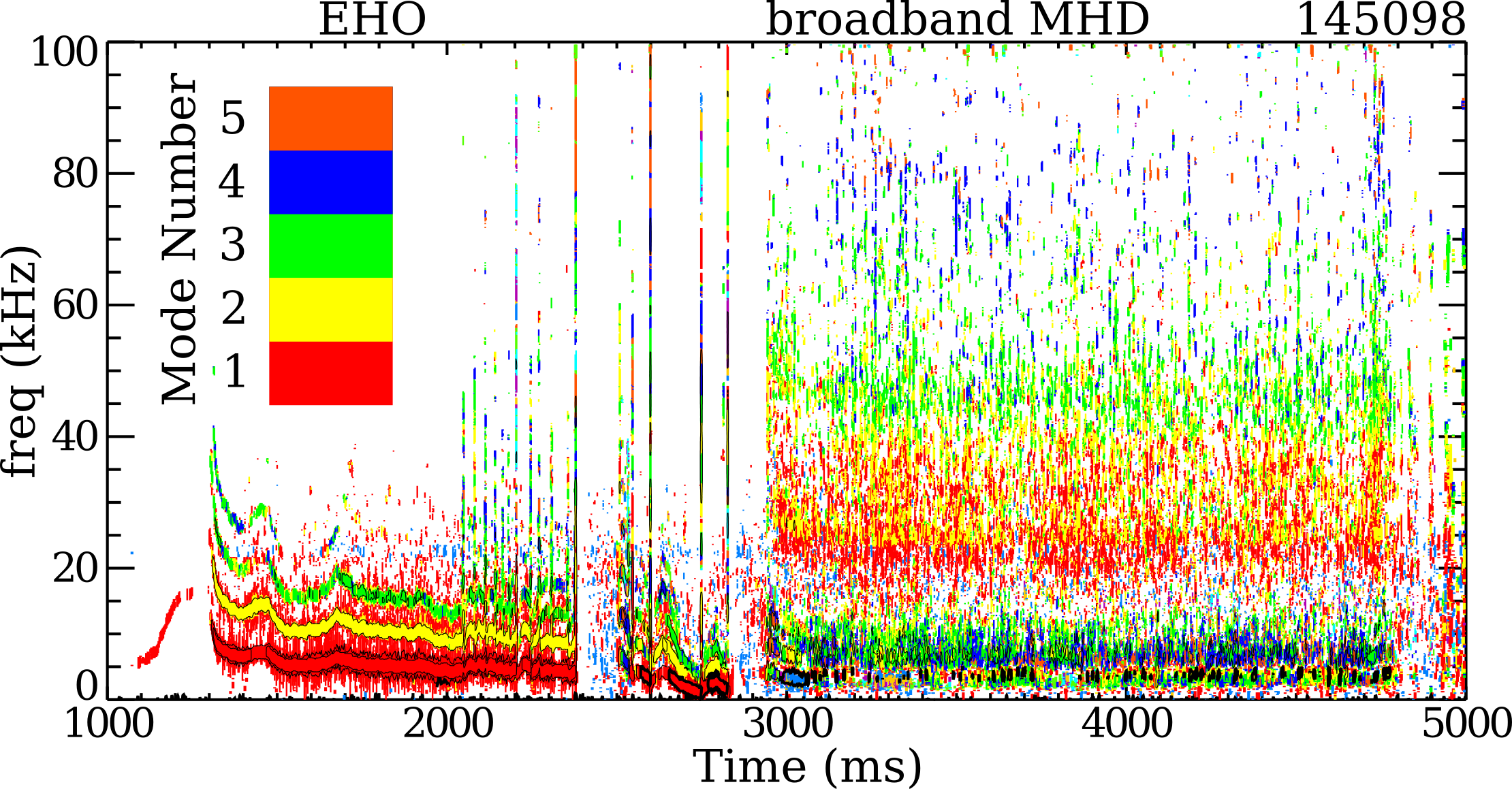
Figure 1: [color online] The cross-power spectrum plot from magnetic-probe measurements from DIII-D shot 145098 shows both an initial phase containing coherent EHO fluctuations, and a subsequent phase with a mix of broadband-MHD and coherent activity.

NIMROD simulations are performed on a DIII-D QH-Mode discharge which exhibits both a phase of coherent edge-harmonic oscillation (EHO) activity and a phase of broadband MHD activity. The cross-power spectrum plot from magnetic probe measurements from DIII-D shot 145098 is shown in Fig. 1. The initial phase of the discharge is dominated by an EHO and later, as the input neutral-beam torque is decreased, a subsequent phase with a mix of broadband-MHD and coherent activity is observed. Relative to QH-mode operation with EHO, operation with broadband MHD tends to occur at higher densities and lower rotation and thus may be more relevant to potential ITER discharge scenarios. We analyze the shot at t=4250 ms where the broadband MHD state has existed for over 1 second. This time period is chosen as it is a low-torque part of the discharge that is relevant to ITER. This is a lower-single-null discharge that predates the discovery of the double-null wide-pedestal QH-mode discharges Burrell et al. (2016); Chen et al. (2017). Before proceeding to the results of our analysis, we discuss the numerical formulation of the problem in the next section (Sec. II).

II Numerical formulation of the problem

The initial 2D condition is a Grad-Shafranov equilibrium, which is a reconstruction of the plasma state as constrained by measurements. A problem arises near the edge as QH-mode discharges typically have large current near the separatrix. EFITLao et al. (1985), the most-widely used code for equilibrium reconstructions, does not ordinarily include current in the scrape-off-layer (SOL). Without SOL current, reconstructions must have one of two undesirable properties: 1) either there is an artificial constraint on the current where it must smoothly vanish at the separatrix, or 2) there is a current discontinuity at the separatrix. The first constraint leads to incorrect gradients in the pedestal region, and the second constraint leads to poor convergence for nonlinear runs. Most importantly, neither constraint gives SOL profiles that are consistent with MHD-force balance.

To ameliorate these issues, our equilibrium solver, nimeq Howell and Sovinec (2014), is extended to include SOL profiles and current. The profiles are extended from the Last Closed Flux Surface (LCFS) into the SOL region. The SOL profiles for this particular case are described in detail in Ref. King et al. (2017a). In Ref. King et al. (2017b), a quantitative analysis of the impact of adding SOL current to the equilibrium is presented. Re-solving the equilibrium and including SOL current and flow has little effect on the linear analysis, but is critical for nonlinear simulations as it eliminates discontinuities in current and flow at the LCFS. These discontinuities produce numerical problems when perturbations are advected over the LCFS. We present details of the configuration of these nonlinear simulations next.

As seen in Figure 1, a time late in the discharge (4250 ms) is chosen to analyze. The simulation therefore starts from a state that is itself a result of the low-$n_{\phi}$ perturbation activity associated with QH-mode. The goal of our simulations is therefore not to understand the onset phase of the broadband activity, but rather is to answer the question: “Is the observed low-$n_{\phi}$ activity calculated by extended MHD consistent with experimental observations?” Because there is some ambiguity in separating external sources and the radial transport that is caused by both macroscopic and microscopic turbulence, the simulations are run such that the sources exactly maintain the equilibrium. Although the simulation is run as an initial-value simulation, it is the (possibly turbulent) steady-state that is of interest. Our simulation formulation is more similar to gyrokinetic turbulence simulations and has similar concerns in terms of statistical validation and temporal convergence issues Holland et al. (2011). One difference with gyrokinetic simulations is that the modes are allowed to generate $n=0$ transport. As long as this transport does not induce changes to the profiles that are far outside the measured constraints, our formulation is accurate and self-consistent.

The simulation is initialized from a linear computation of modes with a restricted toroidal-mode-number range ($n_{\phi}=1-8$). The mode energies at $t=0s$ are small, and the largest energy is contained within the $n_{\phi}=4$ mode that has a spectral kinetic-energy content of $4.2\times 10^{-5}\;J$ and a spectral magnetic-energy content of $4.4\times 10^{-6}\;J$. For the nonlinear runs, a resistive-MHD model with an anisotropic stress tensor and anisotropic thermal heat conduction is used as the computational resources required for two-fluid simulations are currently prohibitive. Although two-fluid nonlinearities could possibly change the nonlinear cascade, the macroscopic nature of this mode means that the MHD model may be sufficiently valid to begin gaining intuition in this regime. As discussed later, two-fluid effects are likely critical for more quantitative understanding.

The resistivity profile is chosen such that the Lundquist number, $S$, in the core is $1.1\times 10^{6}$. This choice of resistivity is enhanced by a factor of 100 relative to the Spitzer value for computational practicality. The model includes large parallel and small perpendicular diffusivities in the momentum and energy equations. Our simulations use $\chi_{\parallel}=10^{8}\;m^{2}/s$. The small perpendicular diffusivities are modeled as isotropic particle, momentum and thermal diffusivities with a magnitude of $1\;m^{2}/s$. Both the resistivity and isotropic viscosity profiles are proportional to $T_{e}^{-3/2}$. The simulation is performed with a $60\times 128$ high-order (bi-quartic) finite-element mesh packed around the pedestal region to resolve the poloidal plane and $24$ Fourier modes in the toroidal direction. The boundary conditions, on both the inner annulus and outer wall, are no-slip for the velocity, Dirichlet for the density and temperature and a perfectly conducting-wall boundary condition for the magnetic field. Linear computations show that the mode growth rates are unaffected by presence of the inner boundary. For our nonlinear computations, the Dirichlet boundary conditions on density and temperature provide an unconstrained source that prevents the edge modes from simply transporting all the stored energy out of the confined plasma region.

III Simulation dynamics with and without flow

Experimentally, it is known that access to the QH-mode regime requires control of the flow profile Garofalo et al. (2011). In particular, large $\mathbf{E}\times\mathbf{B}$ flow shear is correlated with QH-mode operation. In order to ascertain the impact of flow on the nonlinear evolution, we perform simulations with and without steady-state flow.

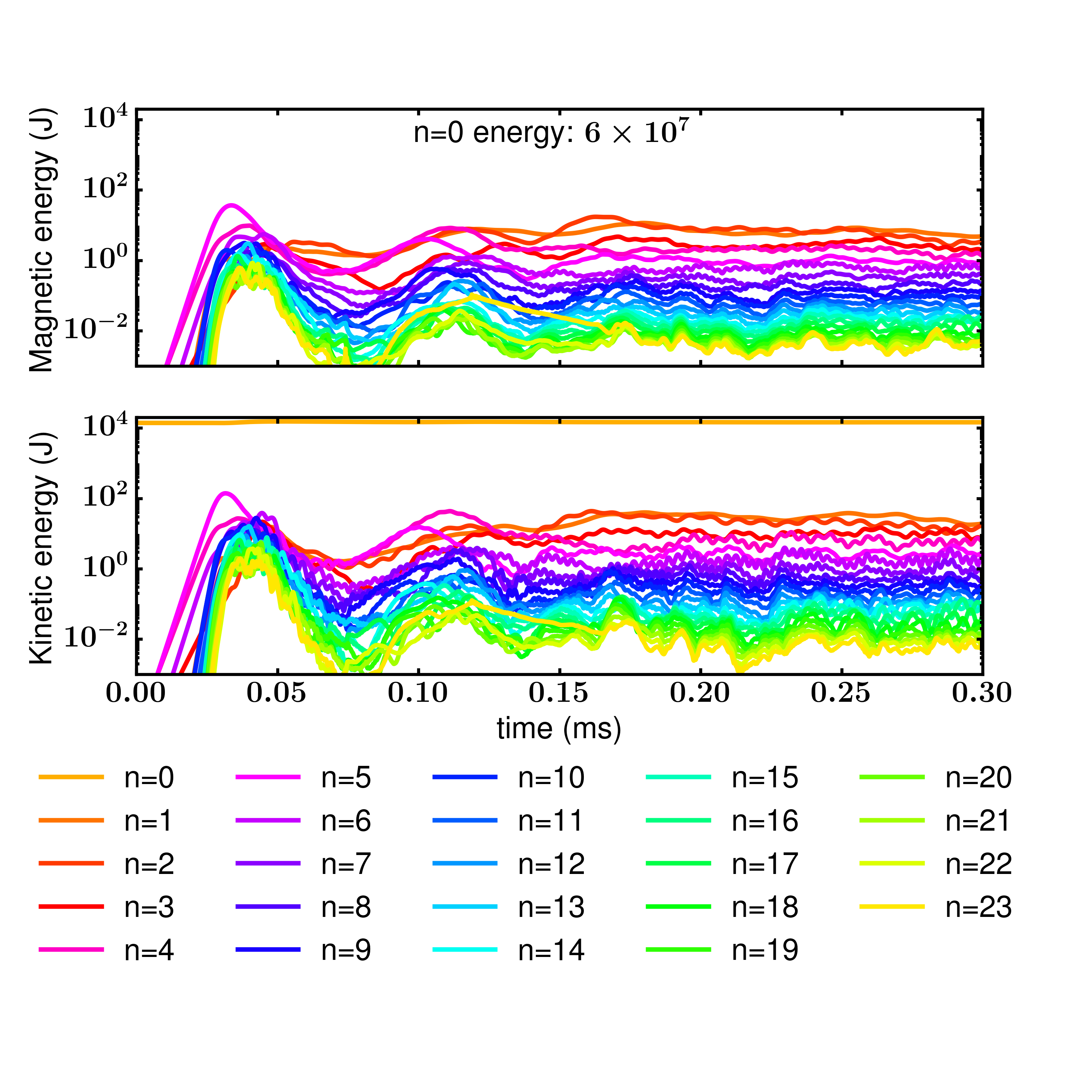
Figure 2: [color online] The time history of the magnetic (top) and kinetic (bottom) energies as decomposed by toroidal mode for a nonlinear simulation with steady-state flow. The simulation ultimately results in a low-$n_{\phi}$ saturated state.

The energy evolution from the nonlinear simulation with steady-state flow, as decomposed by toroidal mode number, of DIII-D QH-mode shot 145098 at $4250\;ms$ is shown in Fig. 2. This simulation includes the toroidal and poloidal rotation profiles inferred from the Carbon impurity species as measured by Charge-Exchange Recombination (CER) spectroscopy. The simulations are initially dominated by a $n_{\phi}=5$ perturbation that saturates at around $30\;\mu s$. After this time a nonlinear saturated quasi-turbulent state develops and the $n_{\phi}=1$ and $2$ perturbations become dominant through an inverse cascade. From $0.15ms$ onwards, modulations are observed in the energy (particularly the kinetic energy) and there is continued interplay between the perturbations. We use the phrase quasi-turbulent as the state is not laminar but it also is not strongly turbulent. If this were a laminar state such as a typical tearing mode case, the perturbed energies would be well-separated and constant in time.

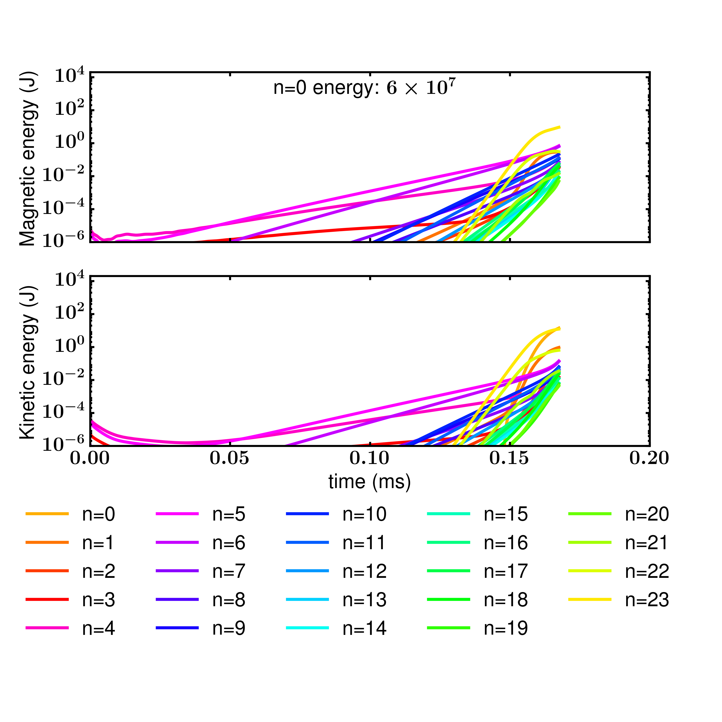
Figure 3: [color online] The time history of the magnetic (top) and kinetic (bottom) energies as decomposed by toroidal mode for a nonlinear simulation without steady-state flow. The dynamics ultimately proceed to high-$n_{\phi}$ and the computation stops when the limit of the spatial resolution is reached.

Simulations without steady-state flow observe an ELM-like high-$n_{\phi}$ evolution. With an identical initial condition as the simulations with flow, the low-$n_{\phi}$ modes are initially stable and later are slowly growing. The dynamics are ultimately overtaken by fast growing high-$n_{\phi}$ modes as shown in Fig. 3. The computation stops when the limit of the spatial resolution is reached. This behavior is similar to extended-MHD simulation of ELM dynamics Pankin et al. (2007); Sugiyama and Strauss (2010); Huijsmans and Loarte (2013), not QH-mode. Importantly, the result that simulations with steady-state flow (and the associated large flow shear) saturate to a low-$n_{\phi}$ state while simulations without steady-state flow (and thus no flow shear) lead to dynamics at high-$n_{\phi}$ is consistent with the experimental observation that QH-mode access requires large-edge flow shear.

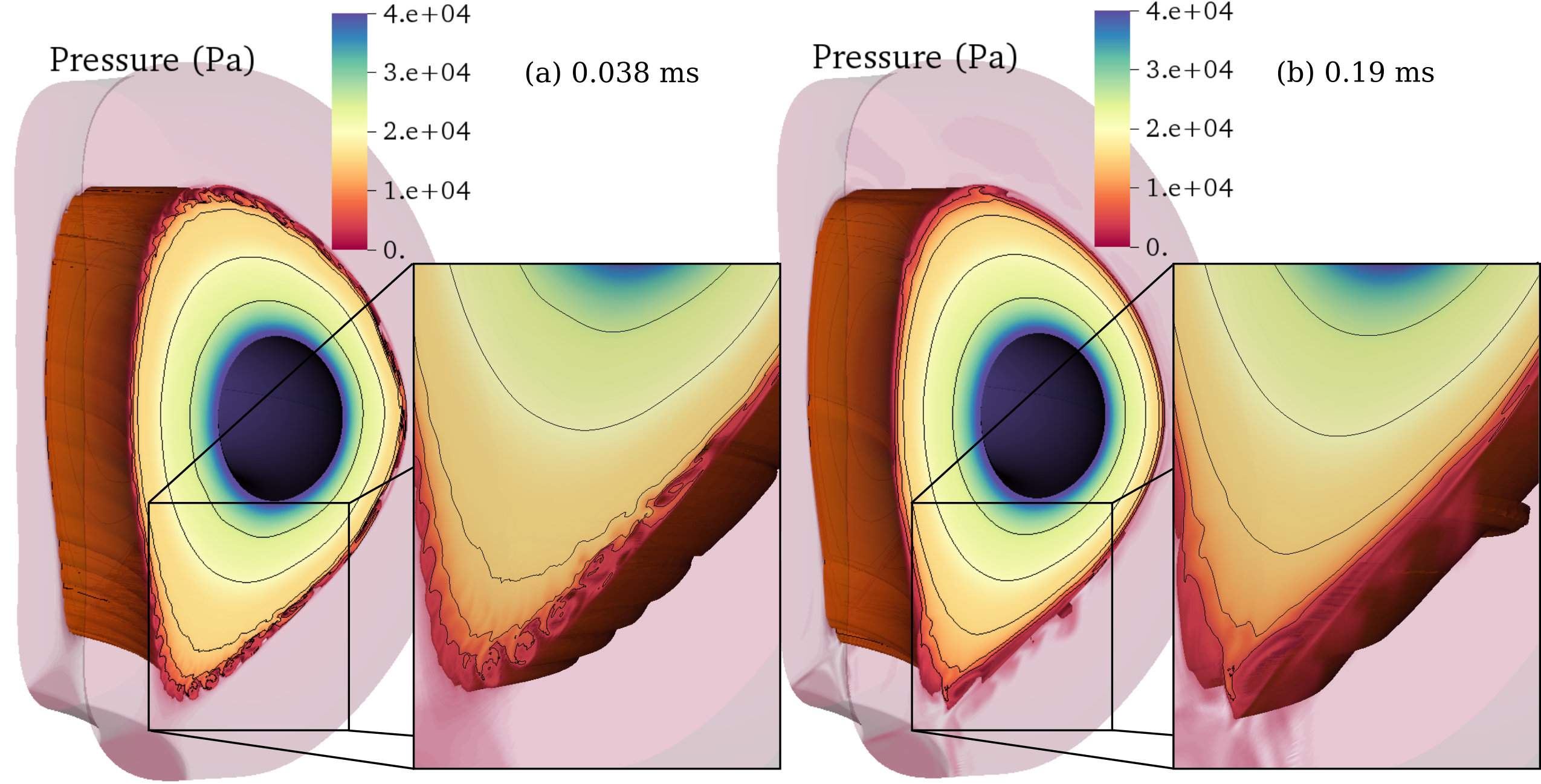
Figure 4: [color online] 3D pressure contours as a cut of the full 3D torus at two different times demonstrate the nonlinear evolution. (a) During the initial stages (t=$38\;\mu s$), dominantly $n_{\phi}=5$ eddies of hot, high density plasma are ejected from the pedestal and are advected poloidally in the counter-clockwise direction while being sheared apart. (b) Later in time (t=$0.19\;ms$), these eddies are sheared apart and a quasi-turbulent steady-state develops that is dominated by low-$n_{\phi}$ perturbations. Fingers of hot plasma form near the x-point in the magnetic-flux expansion region; these are advected poloidally in the counter-clockwise direction and are ultimately sheared apart as they reach the outboard midplane. (Multimedia view)

We turn to analysis of the simulation with steady-state flow for the remainder of the paper. The eddies from the simulation with flow can clearly be seen in Fig. 4. This figure plots 3D pressure contours on a poloidal cut of the full 3D torus at two different time slices to demonstrate the nonlinear evolution. During the initial stages (t=$38\;\mu s$), dominantly $n_{\phi}=5$ eddies of hot, high-density plasma are ejected from the pedestal and are advected poloidally in the counter-clockwise direction while being sheared apart through interaction with both the sub-dominant $n_{\phi}=4$ perturbation and the underlying sheared flow. After this time the perturbation amplitudes are reduced and plots show a smoke-like off-gassing behavior (not shown in figure). Later in time (t=$0.19\;ms$), a quasi-turbulent steady-state develops that is dominated by low-$n_{\phi}$ perturbations. Fingers of hot plasma form near the x-point in the magnetic-flux expansion region, these are advected poloidally in the counter-clockwise direction and are ultimately sheared apart as they reach the outboard midplane similar to theoretical considerations  Guo and Diamond (2015). Figure 4(b) shows both a recently formed finger near the x-point and a highly sheared eddy near the outboard midplane. A video of these dynamics is available with this article. The period of modulation in the spectral energies in Fig. 2 is consistent with the time it takes to form and shear apart the eddies shown in Fig. 4(b).

IV Transport analysis

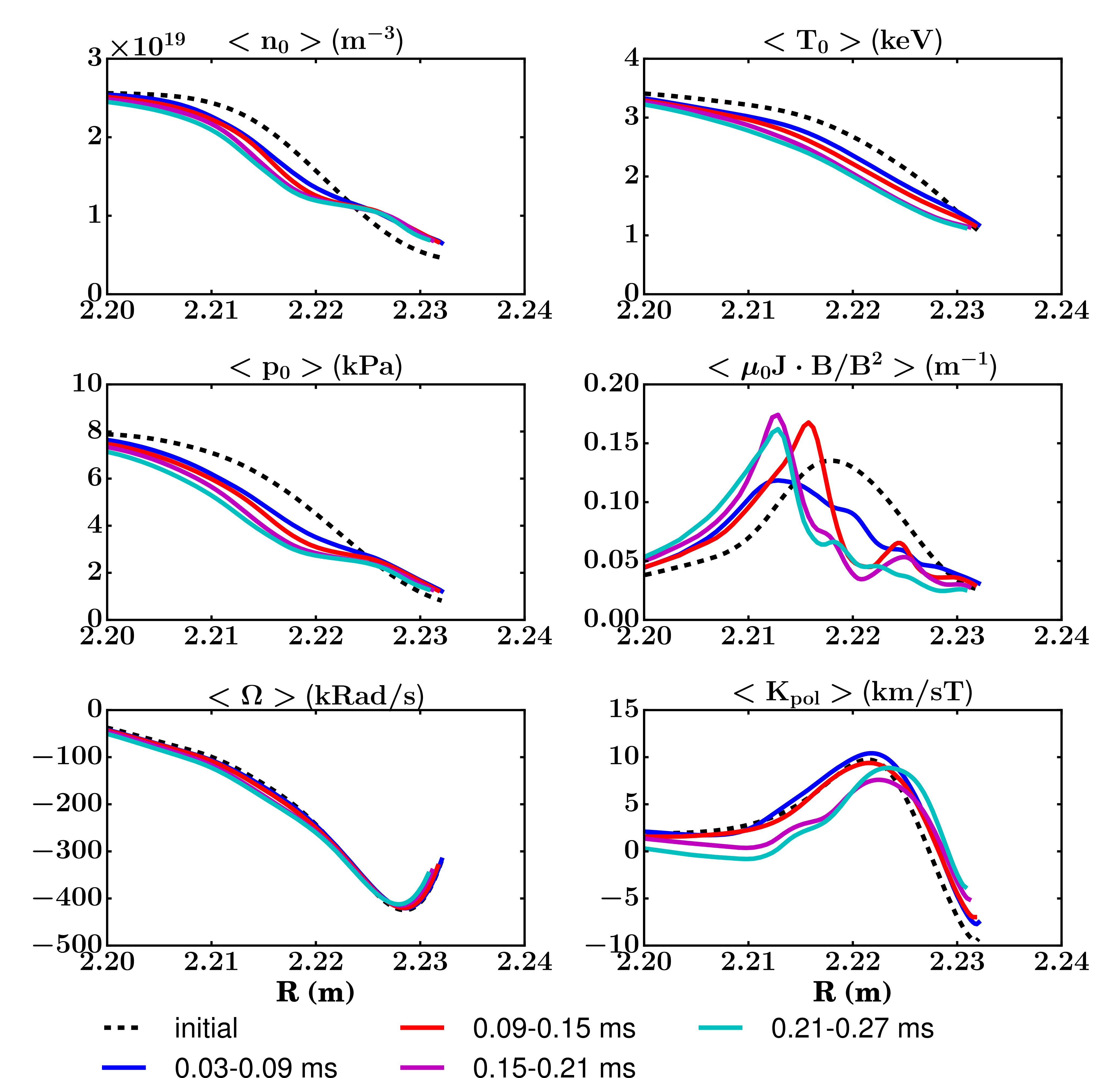
Figure 5: [color online] Flux-surface-averaged values of the density, temperature, pressure, parallel-current density, toroidal rotation frequency and poloidal rotation neoclassical coefficient relative to the location in the pedestal region on the outboard midplane. The initial condition and average values during four time windows are shown.

Having shown that low-$n_{\phi}$ perturbations lead to near steady-state perturbations within the pedestal, it is natural to study the saturation mechanisms and transport in more detail. Figure 5 shows the flux-surface-averaged values of the density, temperature, pressure, parallel-current density, toroidal rotation frequency and poloidal-rotation neoclassical coefficient relative to the location in the pedestal region on the outboard midplane for the initial condition and average values during four time windows. The symmetric flux surfaces associated with the 2D magnetic field are used to determine the surfaces in the flux-surface averages; i.e., we include both the equilibrium and the perturbed $n_{\phi}=0$ contributions. The profiles during the latter two time windows, as associated with the fully saturated state ($>0.15\;ms$ in Fig. 2), are very similar indicating a time-averaged steady 3D solution. The modifications to the flow profiles are small relative to the transport of pressure and current. We thus conclude that the saturation mechanism is related to a flattening of these latter profiles, and not changes to the flow profiles. This turbulent state leads to larger particle transport relative to thermal transport as shown by more flattening of the density profile relative to the temperature profile in Fig. 5, qualitatively consistent with the experimental observations of density pump-out during QH-mode Garofalo et al. (2015). This result is surprising as the magnetic field is stochastic within the pedestal (see Ref. King et al. (2017a)). With the highly anisotropic thermal conduction as included in the model, one would naively expect that thermal transport should be enhanced relative to the particle transport instead of the reverse.

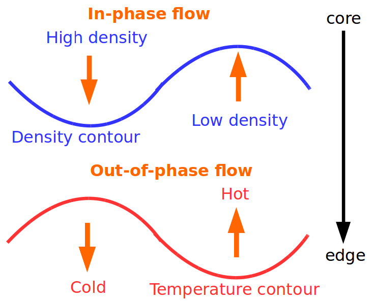
Figure 6: [color online] A schematic showing in-phase flow (arrows) with a density contour and out-of-phase flow (arrows) with a temperature contour.

The transport for density is advective, while temperature includes both convection and anisotropic thermal conduction. The contravariant normal component of the convective flux through a surface, $\Gamma_{f}$, is the flux-surface integral of the product of the density and temperature fluctuations, $\tilde{f}$, and the velocity normal to the surface,

$$\Gamma_{f}=\int\frac{\tilde{f}\tilde{\mathbf{v}}}{\mathbf{B}_{0}\cdot\nabla\theta}\cdot\mathbf{dS}/\int\frac{dS}{\mathbf{B}_{0}\cdot\nabla\theta}\;.$$ (1)

Here $\mathbf{B}_{0}$ is the $n_{\phi}=0$ magnetic field and $\theta$ is a poloidal coordinate. For this quadratic quantity, only mode self-interaction contributes after the application of a toroidal average to the toroidally symmetric surfaces. Importantly for $\Gamma_{T}$ and $\Gamma_{n}$, only the phase and the amplitude of the perturbation relative to the normal velocity may impact the overall normalized magnitude. In Fig. 6, a schematic shows how an in-phase density perturbation leads to enhanced outward (core to edge) transport while an out-of-phase temperature perturbation leads to inward (edge to core) transport. For mixed phases, the overall transport may vanish.

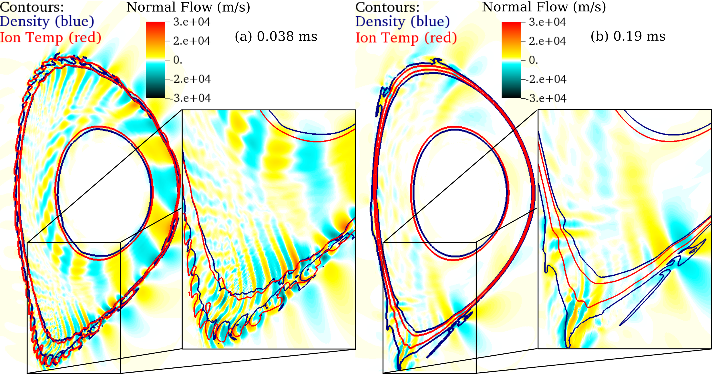
Figure 7: [color online] A poloidal cut of the tokamak at (a) $38\;\mu s$ and (b) $0.19\;ms$ showing three contour lines each of density (blue) and temperature (red) overlaying pseudocolor contours of flow normal to the $n_{\phi}=0$ magnetic field (note the normal flow color scale is adjusted in such a way as to show the global structure of the localized perturbations). Early in time (a), density is in phase with the normal flow while the temperature is out of phase. This effect leads to larger density flux relative to the thermal flux. Later in time (b), a more mixed result is achieved as both the density and temperature are more in phase with the flows, but the large variation in the density contours shows that the amplitude of the density perturbation is larger than that of the temperature perturbation. (Multimedia view)

Figure 7 shows temperature and density contours super-imposed with flux-surface-normal velocity color-plot on a poloidal cut of the tokamak at early and late times during the simulation. Early in time (Fig. 7(a)), density is in phase with the normal flow while the temperature is out of phase. This effect leads to larger density flux relative to the thermal flux. Later in time (Fig. 7(b)), a more mixed result is achieved as both the density and temperature are more in phase with the flows, but the large variation in the density contours shows that the amplitude of the density perturbations is larger than that of the temperature perturbations.

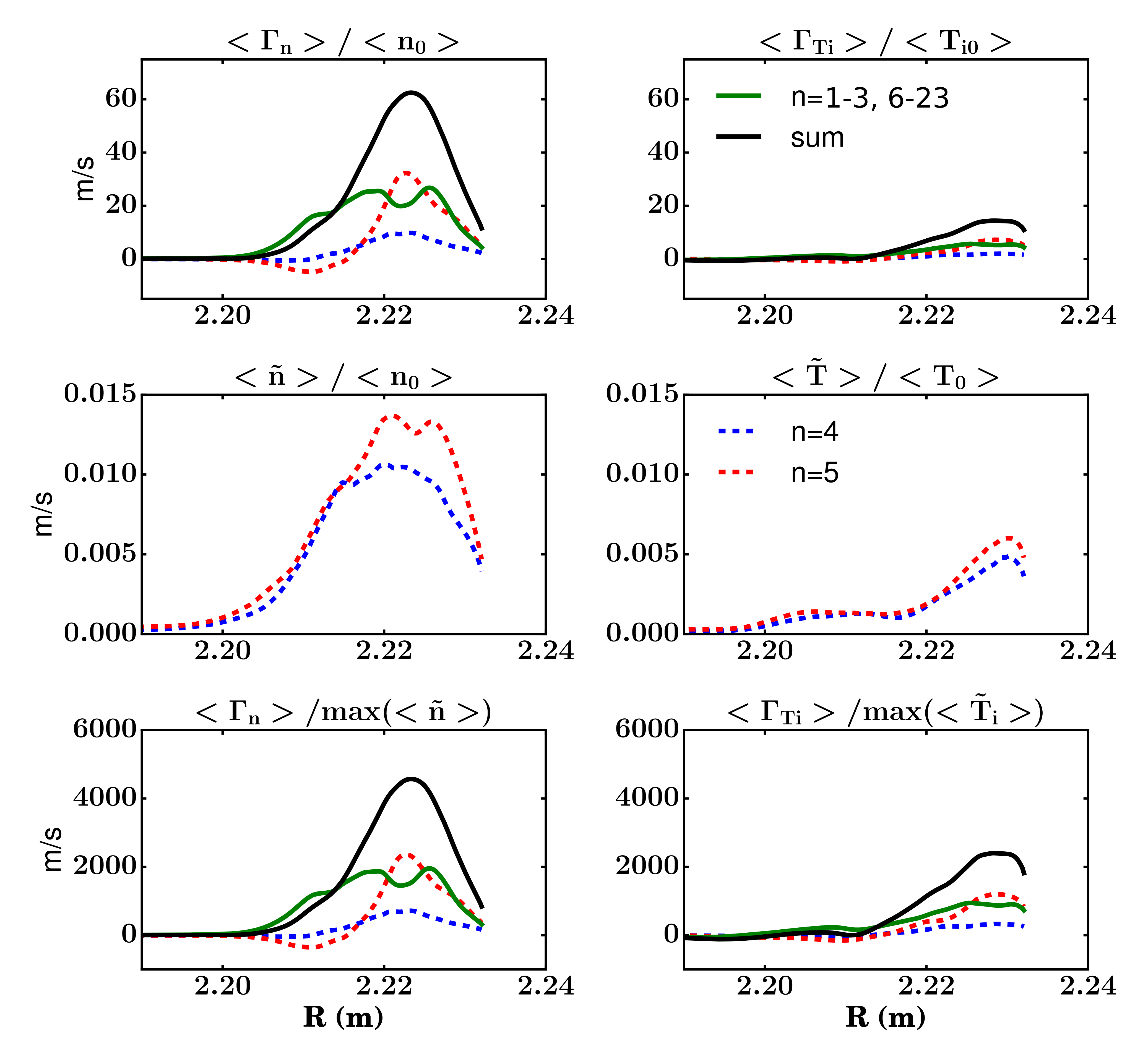
Figure 8: [color online] Flux-surface- and time-averaged ($0.03<t<0.09\;ms$) transport ($\Gamma$), total and broken out by contributions, for density and temperature as normalized to the $n_{\phi}=0$ value at $R=2.22\;m$ on the outboard midplane (top row) and to the maximum perturbation amplitude (bottom row). The middle row displays the flux-surface- and time-averaged density and temperature perturbations. Only the modes associated with the largest perturbations are displayed.

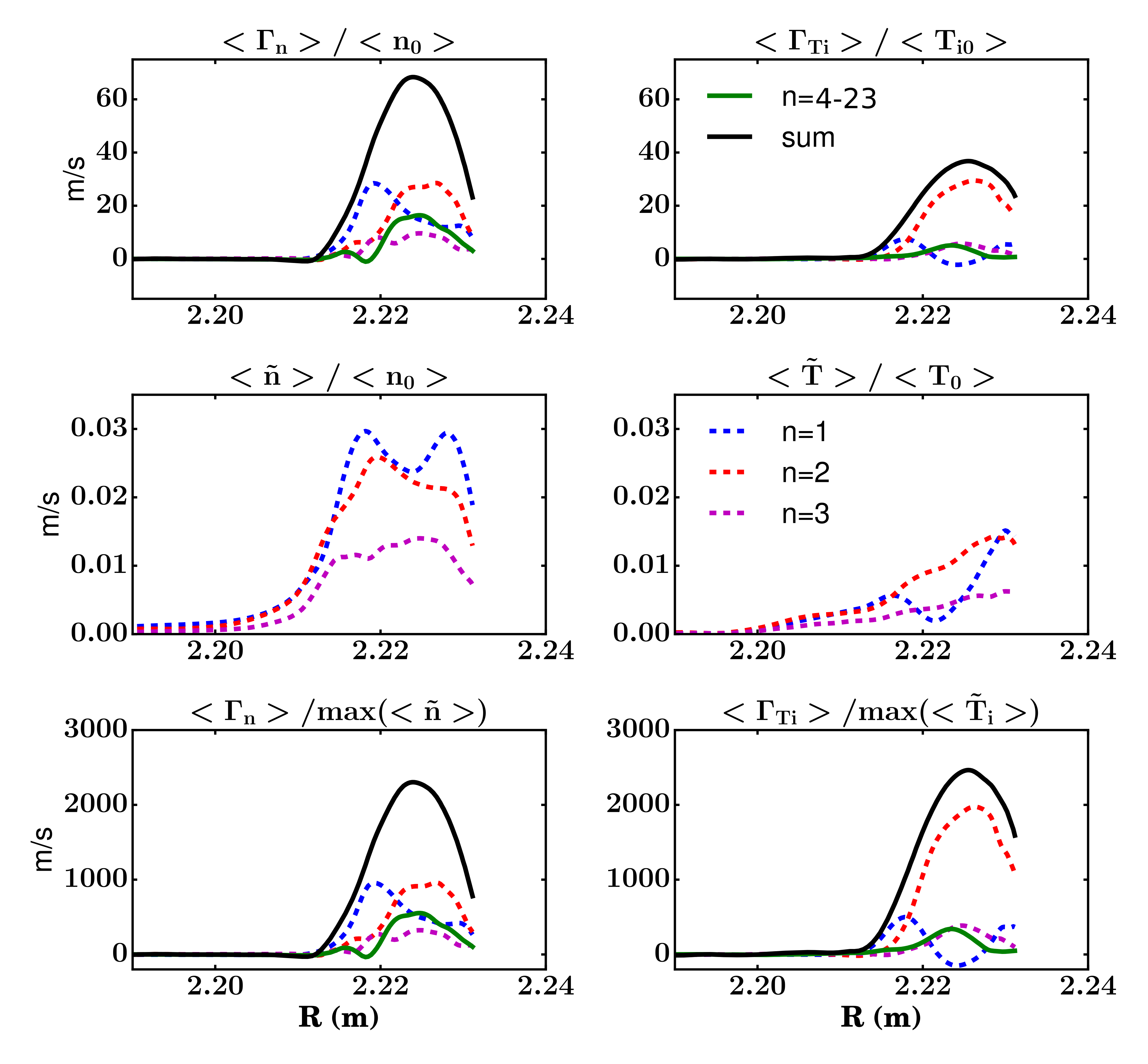
Figure 9: [color online] Flux-surface- and time-averaged ($0.16<t<0.21\;ms$) transport ($\Gamma$), total and broken out by contributions, for density and temperature as normalized to the $n_{\phi}=0$ value at $R=2.22\;m$ on the outboard midplane (top row) and to the maximum perturbation amplitude (bottom row). The middle row displays the flux-surface- and time-averaged density and temperature perturbations. Only the modes associated with the largest perturbations are displayed.

A more rigorous analysis is performed with Figs. 8 and 9. This analysis plots the flux-surface-integrated normalized fluxes and flux-surface-averaged perturbation amplitudes for both density and temperature in time-averaged early (Fig. 8, $0.03<t<0.09\;ms$) and late (Fig. 9, $0.16<t<0.21\;ms$) time windows. Both the total flux and contributions to it from the dominant modes during each time window are shown. The top two figures of each plot show the overall density and temperature convective transport during each window as normalized by the $n_{\phi}=0$ values at $R=2.22\;m$ on the outboard midplane. In both time windows, the density transport is large relative to the thermal transport. It is larger by factors of approximately $6\times$ and $2\times$ in the early and late windows, respectively. The second row of plots compares the normalized perturbation amplitudes, again normalized to the $n_{\phi}=0$ values at $R=2.22\;m$. Consistent with the toroidally decomposed global energy, Fig. 2, the $n_{\phi}=4$ and $5$ perturbations are dominant in the early time window and the $n_{\phi}=1-3$ perturbations are largest during the late time window. For both time windows, the density perturbations are larger than the temperature perturbations by factors of $3\times$ to $2\times$ for the early and late windows, respectively. Thus the difference in amplitude fully accounts for the difference in the fluctuation-induced transport in the late time window, while the early time window still has a factor of approximately $2\times$ that is unaccounted for. The last row of plots shows the convective transport normalized by the maximum perturbation amplitude. This choice of normalization provides an amplitude-independent plot of the effect of the phase. Consistent with estimates from earlier plots, the phase differences contribute a factor of $2\times$ in the early time window while they are negligible in the late time window. This more rigorous analysis shows that both amplitude and phase differences contribute to large fluctuation-induced convective density transport relative to the thermal transport.

More qualitatively, the differences in phase and amplitude arise from differences in the underlying density and temperature equations. The density equation captures the effects of advection and compression and also includes a small numerical diffusivity with coefficient $D_{n}$,

$$\frac{dn}{dt}=-n\nabla\cdot\mathbf{v}+D_{n}\nabla^{2}n\;.$$ (2)

In contrast, the temperature equation differs in factors of the ratio of specific heat, $\Gamma$, and through the inclusion of large anistropic thermal conduction,

$$\frac{n}{\Gamma-1}\frac{dT}{dt}=-nT\nabla\cdot\mathbf{v}+\nabla\cdot n_{0}(\psi_{0})\left(\chi_{\perp}+\chi_{\parallel}\hat{\mathbf{b}}\hat{\mathbf{b}}\cdot\right)\nabla T\;.$$ (3)

The factor of $n(\psi_{0})$ is the density on axis and is used to simplify the specification of the thermal conduction in units of $m^{2}/s$. It can be inferred that differences in the temperature-evolution equation result from differences with the factors of $\Gamma$, and, likely more importantly, the inclusion of anisotropic thermal conduction. The additional terms modify the amplitude and phase relative to the density and reduce the time-averaged fluctuation-induced convective thermal transport when compared to the particle transport.

Of course, the thermal transport is enhanced by anisotropic thermal conduction along the stochastic-magnetic-field lines. As the analysis of the convective transport in the preceding paragraphs appears to explain the differences in the computed density and thermal transport, we expect the conductive transport to be small. In order to ascertain the approximate level of transport we next estimate the confinement times associated with the conductive and convective transport. Using the values of the convective transport during the late time stage (Fig. 9), the convective confinement times for density and temperature are approximately

$$\tau_{conv,n}\simeq\frac{L_{\perp}<n_{0}>}{<\tilde{n}\tilde{v}_{n}>}\simeq 5\times 10^{-4}\;s$$ (4)

and

$$\tau_{conv,T}\simeq\frac{L_{\perp}<T_{0}>}{<\tilde{T}\tilde{v}_{n}>}\simeq 10^{-3}\;s,$$ (5)

respectively. We estimate that $L_{\perp}=0.03\;m$ and $<n_{0}>$ and $<T_{0}>$ are evaluated at $R=2.22\;m$. Phase and amplitude effects are included in the flux-surface-integrated expression in the denominator. The parallel conductive confinement time can be estimated based on the parallel length scale, $L_{\parallel}$, from the magnetic-field puncture plot of Fig. 8 of Ref. King et al. (2017a) of $2500\;m$ as

$$\tau_{cond,\parallel}\simeq\frac{L_{\parallel}^{2}<n_{0}>}{\chi_{\parallel}n_{0}(\psi_{0})}\simeq 1.5\times 10^{-2}\;s,$$ (6)

which is longer than the convective confinement time. The factors of density are added to produce an evaluation of the parallel thermal conduction in the pedestal that is consistent with our temperature-evolution equation (Eqn. (3)). Our parallel conduction model is somewhat crude; however, if we assume that the thermal conduction is in the fastest collisionless limit of free-streaming along field lines, we find that the confinement time is then

$$\tau_{cond,\parallel,vTe}\simeq\frac{L_{\parallel}}{v_{Te}}\simeq 2\times 10^{-3}\;s.$$ (7)

Here a thermal velocity of $v_{Te}=\sqrt{k_{B}T_{e}/m_{e}}\simeq 10^{6}\;m/s$ is used which assumes an electron temperature of $10eV$. This confinement time is comparable to the convective thermal confinement time; however, it is unlikely that collisionless conditions exist near the LCFS and thus the conductive confinement time is likely greater.

V Frequency analysis

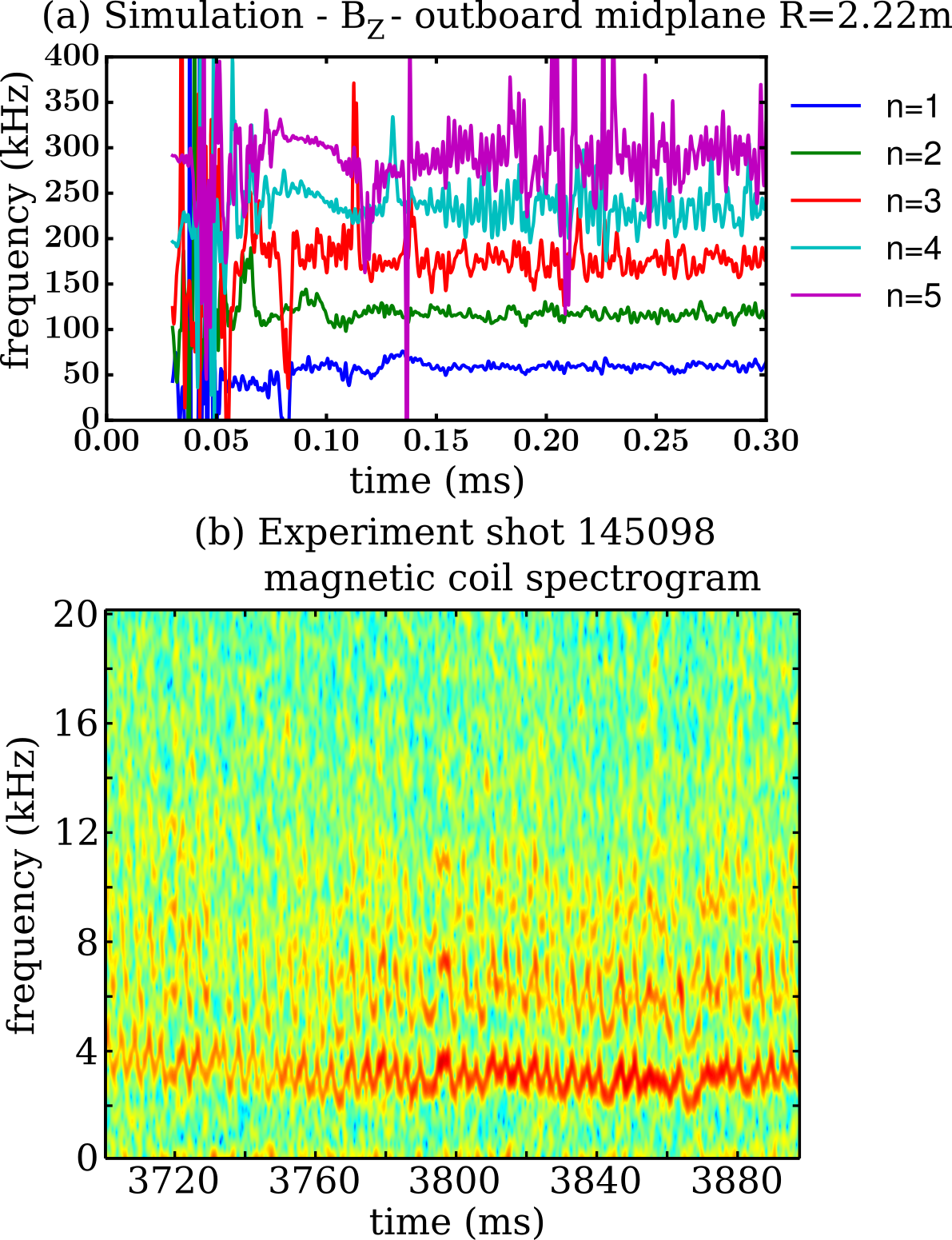
Figure 10: [color online] (a) The frequency of the $\tilde{B}_{Z}$ perturbation as measured by a toroidal set of synthetic probes at $R=2.22\;m$ on the outboard midplane and decomposed by toroidal-mode number relative to (b) a frequency spectrogram produced from a set of magnetic pickup coils at the wall in the experiment. Although we are unable to assign mode numbers to the rotating structures in the experiment, it is clear that the simulated perturbations rotate much faster than those in the experiment.

Figure 10 shows the frequency of the $\tilde{B}_{Z}$ perturbation as measured by a toroidal set of synthetic probes at $R=2.22\;m$ on the outboard midplane and decomposed by toroidal-mode number relative to a frequency spectrogram produced from a set of magnetic pickup coils at the wall in the experiment. Although we are unable to assign mode numbers to the rotating structures in the experiment, which precludes comparison of the amplitude and phase of the perturbations, it is clear that the simulated perturbation rotates much faster than those in the experiment. Our single-fluid computations rotate at approximately the frequency associated with the toroidal ion flow. It is likely that two-fluid effects (e.g. Ref. Coppi (1964); King and Kruger (2014); King et al. (2016)), which are known to modify the frequency through the mediation of the perturbations by both the ion and electron fluids are required to produce dynamics with a more representative frequency. The ion and electron fluids rotate in opposing directions for this discharge. Another possibility is that a drag on resistive wall components modifies the rotation frequency. This effect is not captured by the perfectly conducting wall boundary condition included in the simulation.

VI Discussion

VI.1 Power flow

As QH-mode leads to steady-state pedestal profiles, the fluctuation-induced power flow through the pedestal can be bounded from the experimental data. With the configuration of our present modeling, there is no prior constraint on how much power the perturbations transport through the pedestal. However, we are unable to make this comparison given two limitations of the current model: (1) it uses enhanced dissipation parameters and (2) it does not include Ohmic and viscous heating. The former choice is made for computational practicality while the latter is a natural consequence of the former as the heating rate with enhanced dissipation would be too large. Computations with more realistic dissipation parameters and heating require higher resolution and large computational resources. Additionally, high-resolution computations are currently limited by a time-step restriction that results from the inclusion of flow in the steady state. This restriction requires the time-step size to become smaller as the poloidal resolution is increased. As this time-step restriction is not inherent to NIMROD’s discretization or implicit time-step advance, further work is required to characterize its origin and circumvent it.

VI.2 Sheared eddy hypothesis for QH-mode perturbations

Our simulations are consistent with qualitative features of DIII-D QH-mode; however, further study requires validation with local diagnostics Terry et al. (2008) to determine whether our simulated state more closely resembles broadband MHD or coherent EHO. As explained in Sec. V, it is expected that extensions to the modeling are critical for quantitative comparison which likely requires the correct frequency dependence.

Despite this, the sheared nature of the computed saturated state leads to a hypothesis on the nature of different QH-mode perturbations. We posit that the broadband state is driven similar to the coherent EHO; however, the perturbations are sheared apart before they can reach a sufficient amplitude to form a coherent structure. Additionally, we expect that for moderate flow shear the eddy sizes are of the order of the ion gyroradius or larger, producing rotation in the ion direction. As the shearing rate increases relative to the growth of the instability, it restricts the saturated width of the perturbations to a radial extent that is smaller or on the order of the ion gyroradius. In this regime, the perturbation becomes dominated by the electron dynamics, and it then rotates in the direction of the electron fluid. This is consistent with experimental observations of the coherent EHO rotating in the ion direction, and broadband QH-mode rotating in the electron direction. Two-fluid computations that examine multiple cases with varied low-$n_{\phi}$ perturbations are required to explore this hypothesis further.

VI.3 Limitations of modeling assumptions

Ultimately, it is desired to have a modeling capability that can predict the onset of QH-mode. In such a simulation, the evolution of the 2D fields that comprise our underlying equilibrium are modeled. Presumably, a sufficient demonstration evolves the 2D fields through the stability boundary associated with the 3D modes and tracks the 3D dynamics through saturation. Our present simulation, which assumes the underlying state is static in time, is not able to capture this evolution. This requires a simulation that couples a model of the underlying drives and transport (which is a challenging problem itself, see e.g. Ref. Callen et al. (2010)) that are outside of the present model coupled to the dynamics and fluctuation-induced transport of the MHD model. This is left to future studies.

VII Summary

The simulations shown here have demonstrated the capability of the extended-MHD code NIMROD to model the low-$n_{\phi}$ perturbations associated with QH-mode. With this capability, our longer term goal is to produce a model that is able to determine the feasibility of QH-mode operation in future burning-plasma devices. This goal requires more quantitative validation on a broad set of discharges with varying parameters in addition to more focus on the role of the flow shear in the accessibility criterion for QH-mode.

Our simulations that include the flow profiles inferred from CER Carbon impurity measurements produce a quasi-turbulent state dominated by the low-$n_{\phi}$ perturbations. This state is only achieved after careful inclusion of the reconstructed equilibria including the addition of SOL profiles and associated current. The interplay between driven low-$n_{\phi}$ perturbations and the flow shear prevents the formation of laminar dynamics. Importantly, simulations without flow have dynamics that develop at high-$n_{\phi}$ and do not saturate consistent with experimental observations on the importance of large edge-flow shear to QH-mode access.

Analysis of the transport generated by the low-$n_{\phi}$ perturbations shows that a flattening of the pressure and current profiles is the likely mechanism that eliminates the free-energy drive and leads to saturation. Regarding the modifications to the pressure profile, the particle transport is large relative to thermal transport. Further analysis shows that differences in the particle and thermal fluxes result from a difference in the amplitudes of the density and temperature perturbations as well as phase decorrelation of the temperature with respect to the normal flow. The conclusion is that differences in the temperature-evolution equation resulting from the inclusion of the anisotropic thermal conduction modify the amplitude and phase relative to the density perturbation and reduce the time-averaged convective thermal transport when compared to the particle transport.

References

- Garofalo et al. (2015) A. M. Garofalo, K. H. Burrell, D. Eldon, B. A. Grierson, J. M. Hanson, C. Holland, G. T. A. Huijsmans, F. Liu, A. Loarte, O. Meneghini, T. H. Osborne, C. Paz-Soldan, S. P. Smith, P. B. Snyder, W. M. Solomon, A. D. Turnbull, and L. Zeng, Physics of Plasmas 22, 056116 (2015).
- Connor et al. (1998) J. W. Connor, R. J. Hastie, H. R. Wilson, and R. L. Miller, Physics of Plasmas 5, 2687 (1998).
- Leonard et al. (2006) A. W. Leonard, N. Asakura, J. A. Boedo, M. Becoulet, G. F. Counsell, T. Eich, W. Fundamenski, A. Herrmann, L. D. Horton, Y. Kamada, A. Kirk, B. Kurzan, A. Loarte, J. Neuhauser, I. Nunes, N. Oyama, R. A. Pitts, G. Saibene, C. Silva, P. B. Snyder, H. Urano, M. R. Wade, H. R. Wilson, and f. t. P. a. E. P. I. Group, Plasma Physics and Controlled Fusion 48, A149 (2006).
- Burrell et al. (2005) K. H. Burrell, W. P. West, E. J. Doyle, M. E. Austin, T. A. Casper, P. Gohil, C. M. Greenfield, R. J. Groebner, A. W. Hyatt, R. J. Jayakumar, D. H. Kaplan, L. L. Lao, A. W. Leonard, M. A. Makowski, G. R. McKee, T. H. Osborne, P. B. Snyder, W. M. Solomon, D. M. Thomas, T. L. Rhodes, E. J. Strait, M. R. Wade, G. Wang, and L. Zeng, Physics of Plasmas 12, 056121 (2005).
- Solomon et al. (2014) W. M. Solomon, P. B. Snyder, K. H. Burrell, M. E. Fenstermacher, A. M. Garofalo, B. A. Grierson, A. Loarte, G. R. McKee, R. Nazikian, and T. H. Osborne, Phys. Rev. Lett. 113, 135001 (2014).
- Grierson et al. (2015) B. A. Grierson, K. H. Burrell, R. M. Nazikian, W. M. Solomon, A. M. Garofalo, E. A. Belli, G. M. Staebler, M. E. Fenstermacher, G. R. McKee, T. E. Evans, D. M. Orlov, S. P. Smith, C. Chrobak, C. Chrystal, and D.-D. Team, Physics of Plasmas 22, 055901 (2015).
- Burrell et al. (2016) K. H. Burrell, K. Barada, X. Chen, A. M. Garofalo, R. J. Groebner, C. M. Muscatello, T. H. Osborne, C. C. Petty, T. L. Rhodes, P. B. Snyder, W. M. Solomon, Z. Yan, and L. Zeng, Physics of Plasmas 23, 056103 (2016).
- Chen et al. (2017) X. Chen, K. Burrell, T. Osborne, W. Solomon, K. Barada, A. Garofalo, R. Groebner, N. Luhmann, G. McKee, C. Muscatello, M. Ono, C. Petty, M. Porkolab, T. Rhodes, J. Rost, P. Snyder, G. Staebler, B. Tobias, Z. Yan, and the DIII-D Team, Nuclear Fusion 57, 022007 (2017).
- Sakamoto et al. (2004) Y. Sakamoto, H. Shirai, T. Fujita, S. Ide, T. Takizuka, N. Oyama, and Y. Kamada, Plasma Physics and Controlled Fusion 46, A299 (2004).
- Oyama et al. (2005) N. Oyama, Y. Sakamoto, A. Isayama, M. Takechi, P. Gohil, L. Lao, P. Snyder, T. Fujita, S. Ide, Y. Kamada, Y. Miura, T. Oikawa, T. Suzuki, H. Takenaga, K. Toi, and the JT-60 Team, Nuclear Fusion 45, 871 (2005).
- Solano et al. (2010) E. R. Solano, P. J. Lomas, B. Alper, G. S. Xu, Y. Andrew, G. Arnoux, A. Boboc, L. Barrera, P. Belo, M. N. A. Beurskens, M. Brix, K. Crombe, E. de la Luna, S. Devaux, T. Eich, S. Gerasimov, C. Giroud, D. Harting, D. Howell, A. Huber, G. Kocsis, A. Korotkov, A. Lopez-Fraguas, M. F. F. Nave, E. Rachlew, F. Rimini, S. Saarelma, A. Sirinelli, S. D. Pinches, H. Thomsen, L. Zabeo, and D. Zarzoso, Phys. Rev. Lett. 104, 185003 (2010).
- Suttrop et al. (2005) W. Suttrop, V. Hynönen, T. Kurki-Suonio, P. Lang, M. Maraschek, R. Neu, A. Stäbler, G. Conway, S. Hacquin, M. Kempenaars, P. Lomas, M. Nave, R. Pitts, K.-D. Zastrow, the ASDEX Upgrade team, and contributors to the JET-EFDA workprogramme, Nuclear Fusion 45, 721 (2005).
- Snyder et al. (2007) P. Snyder, K. Burrell, H. Wilson, M. Chu, M. Fenstermacher, A. Leonard, R. Moyer, T. Osborne, M. Umansky, W. West, and X. Xu, Nuclear Fusion 47, 961 (2007).
- Chen et al. (2016) X. Chen, K. Burrell, N. Ferraro, T. Osborne, M. Austin, A. Garofalo, R. Groebner, G. Kramer, N. L. Jr, G. McKee, C. Muscatello, R. Nazikian, X. Ren, P. Snyder, W. Solomon, B. Tobias, and Z. Yan, Nuclear Fusion 56, 076011 (2016).
- Liu et al. (2015) F. Liu, G. Huijsmans, A. Loarte, A. Garofalo, W. Solomon, P. Snyder, M. Hoelzl, and L. Zeng, Nuclear Fusion 55, 113002 (2015).
- King et al. (2017a) J. King, K. Burrell, A. Garofalo, R. Groebner, S. Kruger, A. Pankin, and P. Snyder, Nuclear Fusion 57, 022002 (2017a).
- Sovinec et al. (2004) C. Sovinec, A. Glasser, T. Gianakon, D. Barnes, R. Nebel, S. Kruger, D. Schnack, S. Plimpton, A. Tarditi, and M. Chu, Journal of Computational Physics 195, 355 (2004).
- Lao et al. (1985) L. L. Lao, H. S. John, R. D. Stambaugh, A. G. Kellman, and W. Pfeiffer, Nuclear Fusion 25, 1611 (1985).
- Howell and Sovinec (2014) E. Howell and C. Sovinec, Computer Physics Communications 185, 1415 (2014).
- King et al. (2017b) J. R. King, S. E. Kruger, R. J. Groebner, J. D. Hanson, J. D. Hebert, E. D. Held, and J. R. Jepson, Physics of Plasmas 24, 012504 (2017b), http://dx.doi.org/10.1063/1.4972822 .
- Holland et al. (2011) C. Holland, L. Schmitz, T. L. Rhodes, W. A. Peebles, J. C. Hillesheim, G. Wang, L. Zeng, E. J. Doyle, S. P. Smith, R. Prater, K. H. Burrell, J. Candy, R. E. Waltz, J. E. Kinsey, G. M. Staebler, J. C. DeBoo, C. C. Petty, G. R. McKee, Z. Yan, and A. E. White, Physics of Plasmas 18, 056113 (2011).
- Garofalo et al. (2011) A. Garofalo, W. Solomon, J.-K. Park, K. Burrell, J. DeBoo, M. Lanctot, G. McKee, H. Reimerdes, L. Schmitz, M. Schaffer, and P. Snyder, Nuclear Fusion 51, 083018 (2011).
- Pankin et al. (2007) A. Y. Pankin, G. Bateman, D. P. Brennan, A. H. Kritz, S. Kruger, P. B. Snyder, C. Sovinec, and the NIMROD team, Plasma Physics and Controlled Fusion 49, S63 (2007).
- Sugiyama and Strauss (2010) L. E. Sugiyama and H. R. Strauss, Physics of Plasmas 17, 062505 (2010).
- Huijsmans and Loarte (2013) G. Huijsmans and A. Loarte, Nuclear Fusion 53, 123023 (2013).
- Guo and Diamond (2015) Z. B. Guo and P. H. Diamond, Phys. Rev. Lett. 114, 145002 (2015).
- Coppi (1964) B. Coppi, Physics of Fluids 7, 1501 (1964).
- King and Kruger (2014) J. R. King and S. E. Kruger, Physics of Plasmas 21, 102113 (2014).
- King et al. (2016) J. R. King, A. Y. Pankin, S. E. Kruger, and P. B. Snyder, Physics of Plasmas 23, 062123 (2016).
- Terry et al. (2008) P. W. Terry, M. Greenwald, J.-N. Leboeuf, G. R. McKee, D. R. Mikkelsen, W. M. Nevins, D. E. Newman, D. P. Stotler, T. G. on Verification, Validation, U. B. P. Organization, and U. T. T. Force, Physics of Plasmas 15, 062503 (2008).
- Callen et al. (2010) J. Callen, R. Groebner, T. Osborne, J. Canik, L. Owen., A. Pankin, T. Rafiq, T. Rognlien, and W. Stacey, Nuclear Fusion 50, 064004 (2010).