On a cross-diffusion system arising in image denosing

Abstract

We study a generalization of a cross-diffusion problem deduced from a nonlinear complex-variable diffusion model for signal and image denoising.

We prove the existence of weak solutions of the time-independent problem with fidelity terms under mild conditions on the data problem. Then, we show that this translates on the well-posedness of a quasi-steady state approximation of the evolution problem, and also prove the existence of weak solutions of the latter under more restrictive hypothesis.

We finally perform some numerical simulations for image denoising, comparing the performance of the cross-diffusion model to other well-known demoising methods.

Keywords: cross-diffusion, denoising, Perona-Malik, existence of solutions, simulations.

1 Introduction

A fundamental problem in image analysis is the reconstruction of an original image from an observation, usually to perform subsequent operations on it, such as segmentation or inpainting. In this reconstruction, image denoising is the main task, involving the elimination or reduction of random phenomena -noise- which has been introduced in the image acquisition process due to a number of factors like poor lighting, magnetic perturbances, etc.

Additive white Gaussian noise is surely the most used noise model. In it, we assume that the observation $u_{0}$ is the addition of a ground truth image, $u$, with a zero mean Gaussian random variable, $n$. That is, $u_{0}=u+n$. The problem is then how to recover $u$ from $u_{0}$.

Along the years, many different techniques have been developed to treat with this important technological problem. Just to mention a few well known approaches, we have from variational models such as the ROF model [25], to models based on neighborhoods such as the Bilateral filters [30, 27, 28], based on nonlocal information such as the Nonlocal Means [4], or to methods based on partial differential equations, such as anisotropic diffusion models [1], or the Perona-Malik equation [23].

The Perona-Malik equation has received much attention due to the confluence of the very good denoising performance on the discrete level, the mathematical simplicity of its formulation, and the enormous difficulties to establish the well-posedness of the mathematical problem [19]. It reads as follows:

$${\partial}_{t}u=\operatorname{div}(g\nabla u).$$ (1)

The function $g:\mathbb{R}_{+}\to\mathbb{R}_{+}$ is known as the edge detector, which prevents or induces diffusion according to some criteria. In the most usual model, $g\equiv g(|\nabla u|)$, with $g$ satisfying $g(0)>0$ and $g(s)\to 0$ as $s\to\infty$. Common examples of the edge detector are

$$g(s)=\frac{1}{1+(s/\lambda)^{2}},\quad\text{and}\quad g(s)=\exp\big{(}-\frac{s^{2}}{\lambda^{2}}\big{)},$$ (2)

for some scaling parameter $\lambda>0$. Thus, for large gradients (edges in the image) the diffusion is small and so the edges are preserved. On the contrary, for small gradients (almost flat regions) diffusion is allowed, contributing to the elimination of small perturbances, i.e. denoising the image. Similar results are obtained when the norm of the gradient is replaced by the absolute value of the Laplacian, that is, when considering the edge detector as $g(|\Delta u|)$.

As aforementioned, many efforts have been devoted to prove the well-posedness of the Perona-Malik equation, although many questions remain open. Other efforts have been directed to state well-posed Perona-Malik type problems. In this line, Gilboa et al. [18, 17] introduced the following complex-variable problem: Find $I:[0,T]\times\Omega\to\mathbb{C}$ such that

$${\partial}_{t}I=c\operatorname{div}\big{(}g\nabla I\big{)} \text{in }Q_{T}=(0,T)\times\Omega,$$

$$g\nabla I\cdot\nu=0 \text{on }\Gamma_{T}=(0,T)\times{\partial}\Omega,$$

$$I(0,\cdot)=I_{0} \text{in }\Omega,$$

where $\Omega\subset\mathbb{R}^{m}$ is a bounded smooth domain, ${\partial}\Omega$ its boundary, $\nu$ the exterior unitary normal vector, and $c=\exp(i\theta)$, for some $\theta\in(0,\pi/2)$. Introducing the decomposition of $I$ as the sum of its real and imaginary parts, $I=u_{1}+iu_{2}$, and expanding the above equations, they arrived to the following problem: Find $u_{1},u_{2}:[0,T]\times\Omega\to\mathbb{R}$ such that

$${\partial}_{t}u_{1}-\operatorname{div}\big{(}g(a\nabla u_{1}-b\nabla u_{2})\big{)}=0 \text{in }Q_{T},$$ (3)

$${\partial}_{t}u_{2}-\operatorname{div}\big{(}g(b\nabla u_{1}+a\nabla u_{2})\big{)}=0 \text{in }Q_{T},$$ (4)

$$g\nabla u_{1}\cdot\nu=g\nabla u_{2}\cdot\nu=0 \text{on }\Gamma_{T},$$ (5)

$$u_{1}(0,\cdot)={\rm Re}(I_{0}),~{}~{}u_{2}(0,\cdot)={\rm Im}(I_{0}), \text{in }\Omega,$$ (6)

with $a=\cos\theta$, $b=\sin\theta$. In this denoising model, $I_{0}$ is identified with the initial noisy image, leading to ${\rm Re}(I_{0})=u_{0}$, and ${\rm Im}(I_{0})=0$. Thus, the $u_{1}$ equation establishes the rules of evolution of the noisy image, so $u_{1}$ should be regarded as an image itself. The second equation may be rewritten as

$${\partial}_{t}u_{2}-a\operatorname{div}\big{(}g\nabla u_{2}\big{)}=b\operatorname{div}\big{(}g\nabla u_{1}\big{)},$$ (7)

showing that $u_{2}$ is related to some regularization involving the second order derivatives of $u_{1}$. This motivated Gilboa et al. to, instead of considering an edge detector of the form $g(|\Delta u_{1}|)$, use the detector $g\equiv g(u_{2})$.

The Perona-Malik equation (1) is the pure filtering problem for denoising the original image. When deduced from variational principles, this kind of equations arise as the gradient descent corresponding to the Euler-Lagrange equation satisfied by the minima of certain functional. In this variational framework, evolution equations such as

$${\partial}_{t}u-\operatorname{div}(g\nabla u)=\beta(u-u_{0}),$$

may be used to approximate the true filtered image, solution of

$$-\operatorname{div}(g\nabla u)=\beta(u-u_{0}).$$

Here, the right hand side is the fidelity term, introduced to avoid an excessive smoothing in the denoising procedure, and $\beta>0$ is a constant balancing regularization and fidelity.

The corresponding extension of Gilboa’s et al. model (3)-(6) to its steady state version is: Find $u_{1},u_{2}:\Omega\to\mathbb{R}$ such that

$$-\operatorname{div}\big{(}g(a\nabla u_{1}-b\nabla u_{2})\big{)}=\beta_{1}(u_{10}-u_{1}) \text{in }\Omega,$$ (8)

$$-\operatorname{div}\big{(}g(b\nabla u_{1}+a\nabla u_{2})\big{)}=\beta_{2}(u_{20}-u_{2}) \text{in }\Omega,$$ (9)

$$g\nabla u_{1}\cdot\nu=g\nabla u_{2}\cdot\nu=0 \text{on }{\partial}\Omega,$$ (10)

being $u_{10}$ the original noisy image, and $u_{20}=0$.

The proof of existence of solutions of problem (3)-(6) (with or without fidelity terms) and of problem (8)-(10) may be achieved under several sets of restrictions on the data. We mention here three of such cases, making reference only to the evolution problem. The changes which must be introduced to cover the steady-state problem are straightforward.

Case 1. When $g$ is a positive constant, so that the problem becomes linear. Then, if the resulting diffusion matrix, which may be more general than that in (3)-(6), is definite positive the existence of solutions is a classical result.

Case 2. Under the following restriction on the edge detector: there exists a positive constant $\alpha$ such that $\alpha\leq g(s)\leq\alpha^{-1}$, for all $s\in\mathbb{R}_{+}$. In this case, the following key a priori estimate holds for the standard energies

$$\sum_{i=1}^{2}\Big{(}\int_{\Omega}u_{i}^{2}+\alpha\int_{Q_{T}}|\nabla u_{i}|^{2}\Big{)}\leq\int_{\Omega}u_{i0}^{2},$$ (11)

providing the compactness needed to construct the solution from approximation arguments.

Case 3. When $b=0$ the cross-diffusion is eliminated from the problem. Then, $L^{\infty}$ estimates for $u_{1},~{}u_{2}$ are obtained by standard arguments, making estimate (11) valid. In this line, one can ask whether a change of unknowns in (3)-(6) may lead to a diagonal diffusion system. Assuming the following general form for the diffusion terms

$$-\operatorname{div}\big{(}g(u_{1},u_{2})(a_{i1}\nabla u_{1}+a_{i2}\nabla u_{2})\big{)}$$

one finds that this change is possible, and therefore existence of solutions is granted, if one of the following conditions is satisfied:

1. $a_{12}a_{21}>0$, or

2. $a_{12}a_{21}=0$ and $a_{11}\neq a_{22}$,

Unfortunately, none of them is satisfied by problem (3)-(6), although the second is on the base of the proof of existence of solutions given in [22] for a simplified triangular version of the problem, already proposed by Gilboa et al. [18].

All these special cases have some disadvantages from the image denoising point of view. The linear filtering, as it is well known, produces an over-smoothing which results in the edges of the objects within the image being blurred. In the diagonal or triangular matrix diffusion case, the effects of cross-diffusion are neglected or very mild, and the interpretation of the second component, $u_{2}$, as a regularized version of $\Delta u_{1}$, see (7), does not apply. Finally, considering an edge detector which is a priori bounded away from zero introduces a new parameter, $\alpha$, which must be estimated for a practical implementation of the filter.

In this article we study the model problems (3)-(6) and (8)-(10) without any additional assumptions on the edge detector, $g$, and for a more general form of the diffusion coefficients. Moreover, the possibility of including a fidelity term in the evolution problem (3)-(6) is also treated.

The main result is the proof of existence of weak solutions of the steady state problem, see Theorem 1. This result is instrumental for establishing the well-posedness of a quasi-stationary steady state (QSS) approximation of the (generalized) evolution problem (3)-(6), see Corollary 1. The QSS can be interpreted as a discrete-time gradient descent approximation to the solution of (3)-(6), which we use in Section 3 to illustrate the denoising features of the evolution cross-diffusion model.

However, our $L^{\infty}$ estimates for the QSS approximation depend, in general, on the time discretization step, $\tau$, preventing the passing to the limit $\tau\to 0$ to get a solution of the time continuous problem. In Corollary 2, we summarize the special cases in which an uniform $L^{\infty}$ estimate may be found, and thus the existence of solutions of the evolution problem may be proven.

Let us finally mention that cross-diffusion problems like (3)-(6) appear in many applications in physics, chemistry or biology for describing the time evolution of densities of multi-component systems. A fundamental theory for the study of strongly coupled systems was developed by Amann [2] which established, under suitable conditions, local existence of solutions, which become global if their $L^{\infty}$ and Hölder norms may be controlled.

Since generally no maximum principle holds for parabolic systems, the proof of $L^{\infty}$ bounds is a challenging problem [20], and ad hoc techniques must be employed to deduce the existence of solutions of particular problems. A useful methodology avoiding the $L^{\infty}$ bounds requirement of Amman’s results was introduced in [10] and later generalized in a series of papers, see [7, 8, 11, 9, 12, 20] and the references therein. However, this technique relies on the introduction of a Lyapunov functional needing of a particular cross-diffusion structure which is not satisfied by system (3)-(6). Thus, the proof of existence of solutions of problem (3)-(6) with the edge detector $g$ of the type (2) remains open.

The nonlinear instability of these type of strongly coupled systems, as induced only by cross diffusion terms, has been also an active area of research, see [15, 26, 6, 16] and the references therein. The investigation of this property for systems of the type (3)-(6) will be subject of future research.

2 Main results

We consider the following problems.

Evolution problem: Given a fixed $T>0$ and a bounded domain $\Omega\subset\mathbb{R}^{m}$, find $\mathbf{u}=(u_{1},u_{2})$, with $u_{i}:(0,T)\times\Omega\to\mathbb{R}$, such that, for $i=1,2$,

$${\partial_{t}}u_{i}-\operatorname{div}J_{i}(\mathbf{u})=f_{i}(\mathbf{u}) \quad\text{in }Q_{T},$$ (12)

$$J_{i}(\mathbf{u})\cdot\nu=0 \quad\text{on }\Gamma_{T},$$ (13)

$$u_{i}(\cdot,0)=u_{i0} \quad\text{in }\Omega,$$ (14)

with flow and fidelity functions given by

$$J_{i}(\mathbf{u})=g(\mathbf{u})\big{(}a_{i1}\nabla u_{1}+a_{i2}\nabla u_{2}\big{)},$$ (15)

$$f_{i}(\mathbf{u})=\beta_{i}(u_{i0}-u_{i}),$$ (16)

for $\mathbf{u}_{0}\in L^{\infty}(\Omega)^{2}$, and for some constants $\beta_{i}\geq 0$.

Steady state problem: The steady state corresponding to problem (12)-(14) is found by dropping the time derivative in (12). However, we shall study the following generalization: find $\mathbf{u}=(u_{1},u_{2})$, with $u_{i}:\Omega\to\mathbb{R}$, such that, for $i=1,2$,

$$\gamma_{i}u_{i}-\operatorname{div}J_{i}(\mathbf{u})=G_{i} \quad\text{in }\Omega,$$ (17)

$$J_{i}(\mathbf{u})\cdot\nu=0 \quad\text{on }{\partial}\Omega,$$ (18)

for some functions $G_{i}\in L^{\infty}(\Omega)$, constants $\gamma_{i}>0$, and $J_{i}$ given by (15).

Assumptions on the data. We make the following hypothesis on the data, which we shall refer to as (H):

1. $\Omega\subset\mathbb{R}^{m}$ is a bounded domain with Lipschitz continuous boundary, $\partial\Omega$.

2. The constant matrix $A=(a_{ij})$ satisfies:

   • There exists a constant $a_{0}>0$ such that

     $$\xi^{T}A~{}\xi\geq a_{0}|\xi|^{2}\quad\text{for all }\xi\in\mathbb{R}^{m}.$$

   • The elements of $A$ satisfy $a_{ii}>|a_{ji}|$ for $i,j=1,2$, $i\neq j$.

3. The edge detector $g:\mathbb{R}^{2}\to\mathbb{R}$ is continuous, with $g(K)\subset(0,\infty)$ for all compact $K\subset\mathbb{R}^{2}$.

Theorem 1.

Assume (H), and let $\gamma_{i}>0$, and $G_{i}\in L^{\infty}(\Omega)$, for $i=1,2$. Then, there exists a weak solution $\mathbf{u}\in H^{1}(\Omega)^{2}\cap L^{\infty}(\Omega)^{2}$, of the stationary problem (17)-(18).

The next result establishes the existence of solutions of a time-discrete version of problem (12)-(14) known as the quasi-steady state approximation problem. This is the time discretization scheme we use in our numerical experiments of Section 3.

Corollary 1.

Let $\tau>0$, assume (H), and set $\mathbf{u}^{0}=\mathbf{u}_{0}\in L^{\infty}(\Omega)^{2}$. Then, for all $n\in\mathbb{N}$, there exists a weak solution $\mathbf{u}^{n+1}=(u_{1}^{n+1},u_{2}^{n+1})$, with $u_{i}^{n+1}\in H^{1}(\Omega)\cap L^{\infty}(\Omega)$, of the problem, for $i=1,2$,

$$\frac{1}{\tau}(u_{i}^{n+1}-u_{i}^{n})-\operatorname{div}J_{i}(\mathbf{u}^{n+1})=f_{i}(\mathbf{u}^{n+1}) \quad\text{in }\Omega,$$ (19)

$$J_{i}(\mathbf{u}^{n+1})\cdot\nu=0 \quad\text{on }\partial\Omega.$$ (20)

Finally, from the construction in Theorem 1 , we deduce the existence of solutions of the evolution problem (12)-(14) under some parameter restrictions.

Corollary 2.

Assume (H) and suppose that one of the following conditions is satisfied:

$$(i)~{}a_{12}=a_{21}=0,\quad(ii)~{}a_{12}a_{21}>0,\text{ or }(iii)~{}a_{12}a_{21}=0\text{ and }a_{11}\neq a_{22}.$$

Then, there exists a weak solution $\mathbf{u}=(u_{1},u_{2})$ of the evolution problem (12)-(14), with, for $i=1,2$,

$$u_{i}\in L^{2}(0,T;H^{1}(\Omega))\cap H^{1}(0,T;(H^{1}(\Omega))^{\prime})\cap L^{\infty}(Q_{T}).$$

3 Numerical simulations

In this section we numerically demonstrate the image denoising ability of the evolution cross-diffusion model (12)-(16) in its particular form (3)-(6) considered in Gilboa et al. [18]. For comparison, we use two sets of methods. The first is based on the Perona-Malik (PM) equation which is, as already mentioned, closely related to the cross-diffusion system. With this comparison, we intend to check whether the cross-diffusion system is a clear improvement of the Perona-Malik equation or not.

The second set is based on one step integral filters, among which we have chosen the Bilateral filter (BF) [30, 27, 28] and the Nonlocal Means filter (NLM) [4]. The BF is well-known due to its simplicity and good denoising properties when compared to execution times. The NLM is a clear improvement of the BF regarding denoising quality, and it is one of the state of the art reference method to any denoising algorithm. Comparing to it we also indirectly compare to many other methods which take the NLM as reference [4].

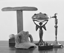
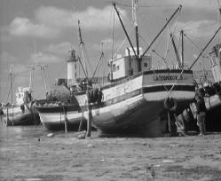
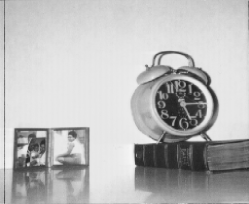
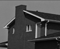
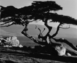
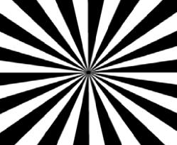
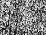
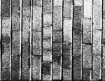
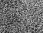
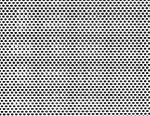
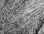
Figure 1: Set of test images. First and second rows are natural images: added value, boat, clock, house, tree, and test. The latter is not natural but it actually behaves as such in the denoising procedure. Third row are texture images: bark, bricks, bubbles, holes, and straw. All of them are of size $512\times 512$ but clock and test, which are $256\times 256$.

The comparison of the methods is done on two classes of intensity images: natural images and texture images, most of them obtained from the SIPI data set, see Figure 1. We add to the original image, $u_{\rm clean}$, a Gaussian white noise to obtain the noisy image, $u_{\rm noisy}$, with fixed signal to noise ratio $\operatorname{SNR}=10$, where

$$\operatorname{SNR}=\frac{\sigma(u_{\rm clean})}{\sigma(u_{\rm clean}-u_{\rm noisy})},$$

being $\sigma$ the standard deviation. After filtering $u_{\rm noisy}$ with each method, we obtain a denoised image, $u_{\rm denoised}$, that we compare to $u_{\rm clean}$ using three quality measures [29]:

• The pick signal to noise ratio (PSNR), given by

  $${\rm PSNR}(u_{1},u_{2})=20\log_{10}\Big{(}\frac{255}{\|u_{1}-u_{2}\|_{2}}\Big{)}.$$

• The normalized cross correlation (NCC), given by

  $${\rm NCC}(u_{1},u_{2})=\frac{\langle u_{1},u_{2}\rangle}{\|u_{1}\|_{2}\|u_{2}\|_{2}}\in[0,1].$$

• The structural similarity (SSIM), given by

  $${\rm SSIM}(u_{1},u_{2})=\frac{(2\mu_{1}\mu_{2}+c_{1})(2\sigma_{1,2}+c_{2})}{(\mu_{1}^{2}+\mu_{2}^{2}+c_{1})(\sigma_{1}^{2}+\sigma_{2}^{2}+c_{2})}\in[0,1],$$

  where $\mu_{i},~{}\sigma_{i},~{}\sigma_{i,j}$ stand for the mean, the standard deviation and the covariance of the corresponding images, and $c_{i}$ are some positive small constants included to avoid instability when the denominators are close to zero.

Since different methods have different sets of structural parameters which must be fixed for actual implementation, we have experimentally optimized them for each image in a reasonable range of values. The optimization has been performed with respect to the PSNR between the original and the denoised images.

3.1 Discretization

We use the well-posed QSS aproximation (19)-(20) of the cross-diffusion problem (12)-(14) to discretize in time. A similar approach is followed for the Perona-Malik equation (1). Then, for the cross-diffusion problem and for the gradient based Perona-Malik equation, that is, when $g\equiv g(|\nabla u|)$, we use the finite element method (FEM) to discretize in space, with linear-wise basis. For the Laplacian based Perona-Malik equation, the use of FEM would require to consider a basis of, at least, piece-wise quadratic polynomials to approximate the second order derivatives. Instead of incrementing the order of the FEM basis, we preferred to use a simpler scheme for this filter, based on the finite differences method.

We give the implementation details for the cross-diffusion system, being that of the Perona-Malik equation similar. Following [18], we fix the initial data as $\mathbf{u}_{0}=(u_{\rm noisy},0)$ and consider the edge detector function as given by

$$g(\mathbf{u})=g(u_{2}),\quad\text{with }g(s)=\exp\big{(}-s^{2}/\lambda_{cd}^{2}\big{)},$$

with $\lambda_{cd}>0$ optimized according to each method and image. The right hand side of (12) is taken as $f_{i}\equiv 0$ (pure filtering case). Finally, like in [18], the diffusion coefficient matrix is taken as, for fixed $\theta\in[0,\pi/2)$,

$$A=\begin{pmatrix}\cos\theta&-\sin\theta\\ \sin\theta&\cos\theta\end{pmatrix},$$

with $\theta=\pi/30$ in the experiments.

We used the open source software deal.II [3] to implement a time semi-implicit scheme with spatial linear-wise finite element discretization. For the time discretization, we take in the experiments a uniform partition of $[0,T]$ of time step $\tau$. For the spatial discretization, we take the natural uniform partition of the rectangle $[0,W]\times[0,H]$, where $W$ and $H$ stand for the width and height (in pixels) of the given image, respectively.

Let, initially, $t=t_{0}=0$ and set $u_{i}^{0}=u_{i0}$. For $n\geq 1$ the problem is: Find $u_{i}^{n}\in S^{h}$ such that for $i=1,2$,

$$\begin{array}[]{l}\frac{1}{\tau}\big{(}u^{n}_{i}-u^{n-1}_{i},\chi)^{h}+\big{(}g(u_{2}^{n})(a_{i1}\nabla u_{1}^{n}+a_{i2}\nabla u_{2}^{n}),\nabla\chi\big{)}^{h}=0,\end{array}$$ (21)

for every $\chi\in S^{h}$, the finite element space of piecewise $\mathbb{Q}_{1}$-elements. Here, $(\cdot,\cdot)^{h}$ stands for a discrete semi-inner product on $\mathcal{C}(\overline{\Omega})$.

Since (21) is a nonlinear algebraic problem, we use a fixed point argument to approximate its solution, $(u_{1}^{n},u_{2}^{n})$, at each time slice $t=t_{n}$, from the previous approximation $u_{i}^{n-1}$. Let $u_{i}^{n,0}=u_{i}^{n-1}$. Then, for $k\geq 1$ the linear problem to solve is: Find $u_{i}^{n,k}$ such that for $i=1,2$, and for all $\chi\in S^{h}$

$$\begin{array}[]{l}\frac{1}{\tau}\big{(}u^{n,k}_{i}-u^{n-1}_{i},\chi)^{h}+\big{(}g(u_{2}^{n,k-1})(a_{i1}\nabla u_{1}^{n,k}+a_{i2}\nabla u_{2}^{n,k}),\nabla\chi\big{)}^{h}=0.\end{array}$$

We use the stopping criteria

$$\max_{i=1,2}\|u_{i}^{n,k}-u_{i}^{n,k-1}\|_{2}<\text{tol},$$ (22)

for values of tol chosen empirically, and set $u_{i}^{n}=u_{i}^{n,k}$. See Algorithm 1 for implementation details.

Turning to the neighborhood one-step filters, we used the simplest version of the Bilateral filter, also known as Yaroslavsky filter [30], given by

$$\operatorname{Y}u(\mathbf{x})=\frac{1}{C(\mathbf{x})}\int_{B_{\rho}(\mathbf{x})}\exp\Big{(}-\frac{|u(\mathbf{x})-u(\mathbf{y})|^{2}}{h^{2}}\Big{)}u(\mathbf{y})d\mathbf{y},$$

where $B_{\rho}(\mathbf{x})$ is a box of diameter $4\rho$ centered at $\mathbf{x}$, and $\rho,~{}h$ are positive parameters. The term $C(\mathbf{x})$ is the normalizing factor

$$C(\mathbf{x})=\int_{B_{\rho}(\mathbf{x})}\exp\Big{(}-\frac{|u(\mathbf{x})-u(\mathbf{y})|^{2}}{h^{2}}\Big{)}d\mathbf{y}.$$

For its implementation, we used the fast algorithm introduced in [24, 13, 14].

The Nonlocal Means filter is defined as

$$\operatorname{NLM}u(\mathbf{x})=\frac{1}{C(\mathbf{x})}\int_{\Omega}\exp\Big{(}-\frac{M_{\sigma}(\mathbf{x},\mathbf{y})}{h^{2}}\Big{)}u(\mathbf{y})d\mathbf{y},$$

with $h>0$, and the normalizing factor

$$C(\mathbf{x})=\int_{\Omega}\exp\Big{(}-\frac{M_{\sigma}(\mathbf{x},\mathbf{y})}{h^{2}}\Big{)}d\mathbf{y}.$$

The nonlocal term, $M_{\sigma}$, is given in convolution form by

$$M_{\sigma}(\mathbf{x},\mathbf{y})=\int_{\mathbb{R}^{2}}G_{\sigma}(\mathbf{z})|u(\mathbf{x}+\mathbf{z})-u(\mathbf{y}+\mathbf{z})|^{2}d\mathbf{z},$$

where $G_{\sigma}$ is a Gaussian of standard deviation $\sigma$. In practice, the parameter $h$ is fixed in terms of $\sigma$, so this method has a single parameter to be optimized. For the discrete implementation, we used the patch-wise approach introduced by the authors [5].

Algorithm 1 FEM-Fixed point method for cross-diffusion problem (21)

1:Noisy image: $u_{noisy}$; Final time: $T$; Time step: $\tau$

2:Diffusion matrix: $a$; Edge detector function: $g$

3:Tolerance $tol$ for the fixed point method; Max. number of fixed point iterations: maxFpIter

4:Spatial domain

5:Compute triangulation, function basis $\varphi$, and massMatrix

6:$\mathbf{u}=(u_{noisy},0)$, $t=0$

7:while $t<T$ do

8:     $t~{}+\!=~{}\tau$

9:     $\mathbf{u}_{old}=\mathbf{u}$, $\mathbf{u}_{fp}=\mathbf{u}$, relDifference = $\infty$, fpIter=0

10:     while relDifference $>$ tol and fpIter $<$ maxFpIter do

11:         fpIter $+\!=$ 1

12:         $\mathbf{u}_{fp,old}=\mathbf{u}_{fp}$

13:         for All cells of the triangulation do

14:              cellMatrix = 0

15:              for All points in each cell do

16:                  $edge=g(u_{fp,old,2})$

17:                  for $\varphi_{i}$’s of cell basis do

18:                       for $\varphi_{j}$’s of cell basis do

19:                           $cellMatrix(i,j)+\!=\tau*edge*a(i,j)*\nabla\varphi_{i}*\nabla\varphi_{j}*area$                                                        

20:              Add cellMatrix contribution to systemMatrix          

21:         systemMatrix $+\!=$ massMatrix

22:         if fpIter = 1 then

23:              RHS = systemMatrix*$\mathbf{u}$          

24:         Solve by LU method: systemMatrix*$\mathbf{u}_{fp}$ = RHS

25:         Compute relative difference between $\mathbf{u}_{fp}$ and $\mathbf{u}_{fp,old}$      

26:      $\mathbf{u}=\mathbf{u}_{fp}$

27: $\mathbf{u}$

3.2 Experiment data and results

	Initial	CD	PM-L	PM-G	BF	NLM
Parameters		$T$, $\lambda_{cd}$	$T$, $\lambda_{pm}$	$T$, $\lambda_{pm}$	$h$, $\rho$	$\sigma$
		added value
Opt. Par.		(0.2, 0.15)	(0.8, 10)	(0.3, 20)	(64, 4)	8
PSNR	31.8618	35.5620	34.0086	36.7013	36.2672	38.4068
NCC	0.9994	0.99975	0.99963	0.9998	0.99978	0.99987
SSIM	0.99503	0.99788	0.99695	0.99838	0.99819	0.99891
		boat
Opt. Par.		(0.1, 0.1)	(0.3, 10)	(0.1, 20)	(12, 3)	5
PSNR	34.7000	36.2916	35.4629	36.4356	36.0391	36.9337
NCC	0.99942	0.9996	0.99952	0.99962	0.99957	0.99966
SSIM	0.99502	0.99653	0.99579	0.99666	0.9963	0.99702
		clock
Opt. Par.		(0.14, 0.15)	(0.5, 10)	(0.3, 20)	(33, 4)	7
PSNR	32.9488	35.5378	34.187	37.0526	36.8077	38.4792
NCC	0.99957	0.99976	0.99968	0.99983	0.99982	0.99988
SSIM	0.99505	0.99726	0.99625	0.99809	0.99796	0.99863
		house
Opt. Par.		(0.13 , 0.15)	(0.5, 10)	(0.2, 20)	(20, 3)	5
PSNR	34.4251	37.0206	35.7168	37.8745	37.7222	39.2158
NCC	0.99859	0.99924	0.99891	0.99937	0.99934	0.99954
SSIM	0.99504	0.99726	0.99608	0.99777	0.99769	0.99838
		test
Opt. Par.		(0.12, 0.1)	(0.3, 10)	(0.3, 25)	(17, 64)	14
PSNR	28.8457	30.1614	29.1625	30.8796	32.5611	33.0273
NCC	0.99874	0.99916	0.9973	0.99928	0.99947	0.99964
SSIM	0.99711	0.99786	0.99408	0.9982	0.99881	0.9989
		tree
Opt. Par.		(0.12, 0.15)	(0.4, 10)	(0.25, 20)	(35, 4)	8
PSNR	31.7344	33.7960	32.5588	34.7020	34.1934	35.2368
NCC	0.99795	0.99874	0.99617	0.99897	0.99884	0.9991
SSIM	0.99517	0.99697	0.99092	0.99756	0.99727	0.99785

Table 1: Optimal parameters and quality results for the set of natural images.

Measure	Initial	CD	PM-L	PM-G	BF	NLM
Parameters		$T$, $\lambda_{cd}$	$T$, $\lambda_{pm}$	$T$, $\lambda_{pm}$	$h$, $\rho$	$\sigma$
		bark
Opt. Par.		(0.02, 0.3)	(0.05, 50)	(0.03, 70)	(12, 6)	8
PSNR	30.8550	31.3764	30.9596	31.3815	30.9778	30.8820
NCC	0.99877	0.99892	0.99873	0.99892	0.99881	0.99878
SSIM	0.99517	0.99566	0.99492	0.99568	0.99528	0.9952
		bricks
Opt. Par.		(0.01, 0.25)	(0.05, 50)	(0.04, 50)	(13, 5)	4
PSNR	30.8471	31.1076	30.975	31.1590	31.1448	30.9597
NCC	0.99878	0.99886	0.99881	0.99887	0.99886	0.99881
SSIM	0.99517	0.9954	0.99522	0.99547	0.99547	0.9953
		bubbles
Opt. Par.		(0.03, 0.1)	(0.05, 30)	(0.04, 40)	(7, 3)	2
PSNR	36.1726	36.8475	36.3222	37.0446	36.3846	36.2160
NCC	0.99944	0.99953	0.99946	0.99955	0.99946	0.99945
SSIM	0.99502	0.99569	0.99515	0.9959	0.99518	0.99507
		holes
Opt. Par.		(0.03, 0.3)	(0.05, 20)	(0.15, 30)	(14, 7)	14
PSNR	29.2774	29.9741	29.2695	29.9926	30.1212	30.1021
NCC	0.999	0.9992	0.99892	0.99916	0.99914	0.9992
SSIM	0.99617	0.99672	0.99584	0.99677	0.99681	0.99686
		straw
Opt. Par.		(0.01, 0.3)	(0.01, 50)	(0.02, 70)	(12, 5)	14
PSNR	30.8735	31.1492	30.8961	31.1175	30.9911	30.8918
NCC	0.99878	0.99886	0.99875	0.99885	0.99881	0.99878
SSIM	0.99518	0.99542	0.99506	0.99541	0.99528	0.9952

Table 2: Optimal parameters and quality results for the set of texture images.

For the cross-diffusion and the Perona-Malik equations, the time step is fixed as $\tau=0.01$, and the tolerance for the fixed point iteration inside each time loop, see (22), is taken as ${\rm tol}=10^{-3}$.

In Table 1 we show the optimal parameters found for each method, in the sense of PSNR maximization, and the resulting quality measures for each image in the set of natural images. For most of these images, the Laplacian based Perona-Malik equation gives the poorest results. The cross-diffusion, the gradient based Perona-Malik equation and the Bilateral (Yaroslavsky) filters give, in general, similar results. The Nonlocal Means filter outperforms the other methods for all the images.

In Table 2 we present the same information for the set of texture images. In this case the results are not conclusive. The relative performance among methods is closer than in the case of natural images and, in fact, the cross-diffusion and the gradient based Perona-Malik equations give the best results for most of the images. However, the denoising capacity of all of them is very limited and the denoising effect is hard to visualize.

In Figure 2 we show a detail of the image added value showing the performance of all the methods for a natural image. In Figure 3 we show the contours plots for a detail of the texture image holes.

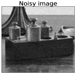
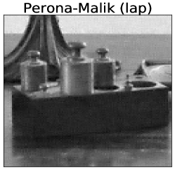
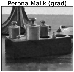
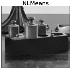
Figure 2: Detail of the natural image added value showing the performance of each method.

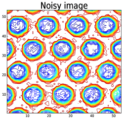
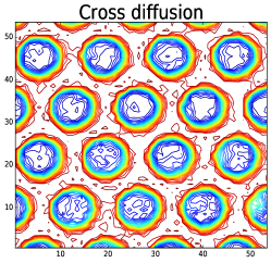
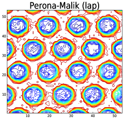
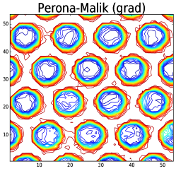
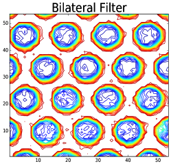
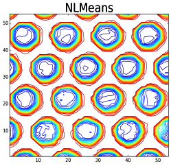
Figure 3: Contours plots for a detail of the texture image holes.

4 Proofs

Proof of Theorem 1. We start considering the following problem: Find $\mathbf{u}:\Omega\to\mathbb{R}^{2}$ such that, for $i=1,2$, and $i\neq j$,

$$\gamma_{i}u_{i}-\frac{\det(A)}{a_{jj}}\operatorname{div}\big{(}g(\mathbf{u})\nabla u_{i}\big{)}=G_{i}-\alpha_{ij}G_{j}+\alpha_{ij}\gamma_{j}u_{j} \quad\text{in }\Omega,$$ (23)

$$g(\mathbf{u})\nabla u_{i}\cdot\nu=0 \quad\text{on }\partial\Omega.$$ (24)

with $\alpha_{ij}=a_{ij}/a_{jj}$. Notice that, due to assumption (H)₂,

$$\det(A)>0,\quad a_{ii}>0,\quad\text{and}\quad|\alpha_{ij}|<1.$$

Step 1: Linearizing. Let $\tilde{\mathbf{u}}\in L^{2}(\Omega)^{2}$ be given and consider the function $g_{k}(s_{1},s_{2})=g(T_{k}(s_{1}),T_{k}(s_{2}))$, with the truncation function $T_{k}:\mathbb{R}\to\mathbb{R}$ given by

$$T_{k}(s)=\left\{\begin{array}[]{ll}-k&\text{if }s\leq-k,\\ s&\text{if }-k\leq s\leq k,\\ k&\text{if }s\geq k.\end{array}\right.$$

Let $\sigma\in[0,1]$. We set the following linear problem: Find $\mathbf{u}\in H^{1}(\Omega)^{2}$ such that for $i=1,2$, and $i\neq j$,

$$\gamma_{i}u_{i}-\frac{\det(A)}{a_{jj}}\operatorname{div}\big{(}g_{k}(\tilde{\mathbf{u}})\nabla u_{i}\big{)}=\sigma(G_{i}-\alpha_{ij}G_{j})+\alpha_{ij}\gamma_{j}u_{j} \quad\text{in }\Omega,$$ (25)

$$g_{k}(\tilde{\mathbf{u}})\nabla u_{i}\cdot\nu=0 \quad\text{on }\partial\Omega.$$ (26)

Since, $g_{k}(\mathbb{R}^{2})\subset g(K)$, with $K=[-k,k]\times[-k,k]$, and by assumption (H)₃, $g(K)\subset(0,\infty)$, that is, the problem is uniformly elliptic, we may apply [21][Chapter 6, Theorem 2.1], to deduce the existence of a unique weak solution $\mathbf{u}\in H^{1}(\Omega)^{2}\cap L^{\infty}(\Omega)^{2}$ of problem (25)-(26).

We now show that the $L^{\infty}(\Omega)$ bound does not depend on $\tilde{\mathbf{u}}$ or $k$. Let $[s]_{+}$ and $[s]_{-}$ denote the positive and negative parts of $s$, so that $s=[s]_{+}-[s]_{-}$. Taking, for $p\geq 1$, $[u_{i}]_{+}^{p}\in H^{1}(\Omega)$ as test function in the weak formulation of (25)-(26), and using Young’s inequlity, we deduce

$$\gamma_{i}\|[u_{i}]_{+}\|_{p+1}\leq\sigma\big{(}\|G_{i}\|_{p+1}+|\alpha_{ij}|\|G_{j}\|_{p+1}\big{)}+\gamma_{j}|\alpha_{ij}|\|[u_{j}]_{+}\|_{p+1}.$$

Summing for $i,j=1,2$, with $i\neq j$, we obtain

$$\gamma_{1}(1-|\alpha_{21}|) \|[u_{1}]_{+}\|_{p+1}+\gamma_{2}(1-|\alpha_{12}|)\|[u_{2}]_{+}\|_{p+1}$$

$$\leq\sigma\big{(}1+|\alpha_{21}|\big{)}\|G_{1}\|_{p+1}+\sigma\big{(}1+|\alpha_{12}|\big{)}\|G_{2}\|_{p+1}$$

A similar estimate holds for $[u_{i}]_{-}^{p+1}$, so we obtain, taking the limit $p\to\infty$,

$$\gamma_{1}(1-|\alpha_{21}|)\|u_{1}\|_{\infty}+ \gamma_{2}(1-|\alpha_{12}|)\|u_{2}\|_{\infty}$$

$$\leq\sigma\big{(}1+|\alpha_{21}|\big{)}\|G_{1}\|_{\infty}+\sigma\big{(}1+|\alpha_{12}|\big{)}\|G_{2}\|_{\infty}.$$ (27)

Step 2: Fixed point. Consider the operator $P:L^{2}(\Omega)^{2}\times[0,1]\to L^{2}(\Omega)^{2}$ given by $P(\tilde{\mathbf{u}},\sigma)=\mathbf{u}$, being $\mathbf{u}$ the solution of the linear problem (25)-(26) corresponding to $(\tilde{\mathbf{u}},\sigma)$. We check that $P$ satisfies the conditions of the Leray-Schauder’s Fixed Point theorem, that is

1. $P$ is continuous and compact.

2. $P(\mathbf{v},0)=0$ for all $\mathbf{v}\in L^{2}(\Omega)^{2}$.

3. The fixed points of $P$ are uniformly bounded in $L^{2}(\Omega)^{2}$.

1. Let $\mathbf{v}_{n}\in L^{2}(\Omega)$ be a sequence strongly convergent to $\mathbf{v}\in L^{2}(\Omega)$, and $\sigma_{n}\to\sigma$. Define $\mathbf{u}_{n}=P(\mathbf{v}_{n},\sigma_{n})$. Using $u_{i,n}\in H^{1}(\Omega)$ as a test function in the weak formulation of (25)-(26) leads to

$$\gamma_{i}\int_{\Omega}|u_{i,n}|^{2}+\frac{\det(A)}{a_{jj}}\min(g(K))\int_{\Omega}|\nabla u_{i,n}|^{2}\leq \sigma_{n}\int_{\Omega}(|G_{i}|+|\alpha_{ij}||G_{j}|)|u_{i,n}|$$

$$+|\alpha_{ij}|\int_{\Omega}|u_{i,n}||u_{j,n}|.$$ (28)

We first use Hölder’s inequality to deduce, after summing for $i,j=1,2$, with $i\neq j$

$$\gamma_{1}(1-|\alpha_{21}|) \|u_{1}\|_{2}^{2}+\gamma_{2}(1-|\alpha_{12}|)\|u_{2}\|_{2}^{2}$$

$$\leq\sigma_{n}\big{(}1+|\alpha_{21}|\big{)}\|G_{1}\|_{2}^{2}+\sigma_{n}\big{(}1+|\alpha_{12}|\big{)}\|G_{2}\|_{2}^{2},$$

and then, from (28), we also deduce that $\|\nabla u_{i,n}\|_{2}$ is uniformly bounded. Therefore, there exists a subsequence of $\mathbf{u}_{n}$ (not relabeled), and a function $\mathbf{u}\in H^{1}(\Omega)^{2}$, such that

$$\nabla u_{i,n}\rightharpoonup\nabla u_{i} \text{weakly in }L^{2}(\Omega),$$

$$u_{i,n}\to u_{i} \text{strongly in }L^{2}(\Omega).$$

Since, by assumption, $v_{i,n}\to v_{i}$ in $L^{2}(\Omega)$ (and a.e. in $\Omega$, for a subsequence), and $\|g_{k}(v_{i,n})\|_{\infty}$ is uniformly bounded with respect to $n$, we deduce by the dominated convergence theorem that $g_{k}(v_{i,n})\to g_{k}(v_{i})$ in $L^{q}(\Omega)$, for all $q<\infty$. Therefore,

$$g_{k}(\mathbf{v}_{n})\nabla u_{i,n}\rightharpoonup g_{k}(\mathbf{v})\nabla u_{i}\quad\text{weakly in }L^{\gamma}(\Omega)$$

for any $\gamma<2$. But since the sequence $g_{k}(\mathbf{v}_{n})\nabla u_{i,n}$ is bounded in $L^{2}(\Omega)$, we deduce that, in fact,

$$g_{k}(\mathbf{v}_{n})\nabla u_{i,n}\rightharpoonup g_{k}(\mathbf{v})\nabla u_{i}\quad\text{weakly in }L^{2}(\Omega).$$

The other terms in the weak formulation of (25)-(26) (with the replacements $\tilde{\mathbf{u}}=\mathbf{v}_{n}$, $\mathbf{u}=\mathbf{u}_{n}$, and $\sigma=\sigma_{n}$) pass clearly to their corresponding limits. Finally, the uniqueness of solutions of problem (25)-(26) implies that the whole sequence $\mathbf{u}_{n}$ converges to $\mathbf{u}$. So the continuity follows. The compactness is directly deduced from the compact embedding $H^{1}(\Omega)\subset L^{2}(\Omega)$.

2. If $\mathbf{u}=P(\mathbf{v},0)$ then, in particular, $\mathbf{u}$ satisfies estimate (27) with $\sigma=0$. Thus, $\mathbf{u}=0$ a.e. in $\Omega$.

3. If $\mathbf{u}=S(\mathbf{u},\sigma)$, we again use that $\mathbf{u}$ satisfies (27) with $\sigma\in[0,1]$, to get the uniform bound of $\mathbf{u}$ in $L^{2}(\Omega)$.

Thus, the Leray-Schauder’s fixed point theorem ensures the existence of a fixed point, $\mathbf{u}$, of $P(\mathbf{u},1)$, which is a solution of (23)-(24) with $g$ replaced by $g_{k}$. But since this fixed point satisfies the $L^{\infty}(\Omega)$ bound (27) (with $\sigma=1$), we deduce that for $k$ large enough $g_{k}(\mathbf{u})=g(\mathbf{u})$, and thus $\mathbf{u}$ is a solution of (23)-(24).

Step 3: Solution of the original problem (17)-(18). The weak solution, $\mathbf{u}$, of problem (23)-(24) satisfies, for all $\varphi\in H^{1}(\Omega)$,

$$\gamma_{1}\int_{\Omega}u_{1}\varphi+\frac{\det(A)}{a_{22}}\int_{\Omega}g(\mathbf{u})\nabla u_{1}\cdot\nabla\varphi=\int_{\Omega}G_{1}\varphi-\alpha_{12}\int_{\Omega}G_{2}\varphi+\alpha_{12}\gamma_{2}\int_{\Omega}u_{2}\varphi,$$

$$\gamma_{2}\int_{\Omega}u_{2}\varphi+\frac{\det(A)}{a_{11}}\int_{\Omega}g(\mathbf{u})\nabla u_{2}\cdot\nabla\varphi=\int_{\Omega}G_{2}\varphi-\alpha_{21}\int_{\Omega}G_{1}\varphi+\alpha_{21}\gamma_{1}\int_{\Omega}u_{1}\varphi.$$

Multiplying the first equation by $a_{11}a_{22}/\det(A)$, the second by $a_{12}a_{11}/\det(A)$ and adding the results leads to

$$\gamma_{1}\int_{\Omega}u_{1}\varphi+\int_{\Omega}g(\mathbf{u})(a_{11}\nabla u_{1}+a_{12}\nabla u_{2})\cdot\nabla\varphi=\int_{\Omega}G_{1}\varphi.$$

A similar combination, also gives

$$\gamma_{2}\int_{\Omega}u_{2}\varphi+\int_{\Omega}g(\mathbf{u})(a_{21}\nabla u_{1}+a_{22}\nabla u_{2})\cdot\nabla\varphi=\int_{\Omega}G_{2}\varphi,$$

so $\mathbf{u}$ is a weak solution of (17)-(18). $\Box$

Proof of Corollary 1. The proof follows easily from Theorem 1 by taking $\gamma_{i}=\beta_{i}+1/\tau>0$ and, recursively, $G_{i}=\beta_{i0}u_{i0}+u_{i}^{n}/\tau\in L^{\infty}(\Omega)$. $\Box$

Remark 1.

The $L^{\infty}$ bound (27) of the steady state problem translates, in the case of the QSS approximation, to

$$\|u_{1}^{n+1}\|_{\infty}+\|u_{2}^{n+1}\|_{\infty}\leq C_{1}\big{(}\|u_{1}^{n}\|_{\infty}+\|u_{2}^{n}\|_{\infty}\big{)}+C_{2}\big{(}\|u_{10}\|_{\infty}+\|u_{20}\|_{\infty}\big{)},$$

with $C_{1}>1$ unless $\alpha_{12}=\alpha_{21}=0$, that is, $a_{12}=a_{21}=0$. Thus, this bound is not useful for passing to the limit $\tau\to 0$, and thus to prove the existence of the evolution problem, except when $A$ is diagonal.

Proof of Corollary 2.

Case 1: $a_{12}=a_{21}=0$ (diagonal case). Consider the time discretization (19)-(20), for which the existence of a solution $\mathbf{u}^{n+1}$ is guaranteed by Corollary 1. In this case, a finer $L^{\infty}$ estimate of each time slice may be obtained. Indeed, the $L^{p+1}$ estimate (27) of Step 1 of the proof of Corollary 1 reduces to

$$(1+\tau\beta_{i})\|u_{i}^{n+1}\|_{p+1}\leq\|u_{i}^{n}\|_{p+1}+\tau\beta_{i}\|u_{10}\|_{p+1},$$

and thus we get

$$\|u_{i}^{n+1}\|_{\infty}\leq\frac{1}{1+\tau\beta_{i}}\|u_{i}^{n}\|_{\infty}+\frac{\tau\beta_{i}}{1+\tau\beta_{i}}\|u_{i0}\|_{\infty}.$$

Solving this differences inequality, we find the required uniform $L^{\infty}$ estimate for proving the convergence of time interpolators. Indeed, observe that this uniform estimate also implies a uniform estimate for $\|\nabla u_{i}^{n+1}\|_{2}$, since by assumption $g(\mathbf{u}^{n+1})$ remains bounded away from zero for all $n\in\mathbb{N}$.

Time interpolators and passing to the limit $\tau\to 0$. This step is somehow standard, so we give an sketch. We define, for $(t,x)\in(t_{n},t_{n+1}]\times\Omega$, the piecewise constant and piecewise linear interpolators

$$u_{i}^{(\tau)}(t,x)=u_{i}^{n+1}(x),\quad\tilde{u}_{i}^{(\tau)}(t,x)=u_{i}^{n}(x)+\frac{t-t_{n}}{\tau}(u_{i}^{n+1}(x)-u_{i}^{n}(x)).$$

Using the uniform estimates of $\|u_{i}^{n+1}\|_{\infty}$ and $\|\nabla u_{i}^{n+1}\|_{2}$, we deduce the corresponding uniform estimates for $\|u_{i}^{(\tau)}\|_{L^{\infty}(Q_{T})}$, $\|\tilde{u}_{i}^{(\tau)}\|_{L^{\infty}(Q_{T})}$, and for

$$\|\nabla u_{i}^{(\tau)}\|_{L^{2}(Q_{T})},\quad\|\nabla\tilde{u}_{i}^{(\tau)}\|_{L^{2}(Q_{T})}\quad\|{\partial}_{t}\tilde{u}_{i}^{(\tau)}\|_{L^{2}(0,T;(H^{1}(\Omega))^{\prime})},$$

implying the existence of $u_{i}\in L^{2}(0,T;H^{1}(\Omega))\cap L^{\infty}(\Omega)$ and

$$\tilde{u}_{i}\in L^{2}(0,T;H^{1}(\Omega))\cap H^{1}(0,T;(H^{1}(\Omega))^{\prime})\cap L^{\infty}(\Omega)$$

such that, at least in a subsequence (not relabeled), as $\tau\to 0$,

$$u_{i}^{(\tau)}\to u_{i}\quad\text{weakly in }L^{2}(0,T;H^{1}(\Omega)),$$ (29)

$$u_{i}^{(\tau)}\to u_{i}\quad\text{weakly* in }L^{\infty}(Q_{T})),$$

$$\tilde{u}_{i}^{(\tau)}\to\tilde{u}_{i}\quad\text{weakly in }H^{1}(0,T;(H^{1}(\Omega))^{\prime}),$$ (30)

$$\tilde{u}_{i}^{(\tau)}\to\tilde{u}_{i}\quad\text{weakly in }L^{2}(0,T;H^{1}(\Omega)),$$ (31)

$$\tilde{u}_{i}^{(\tau)}\to\tilde{u}_{i}\quad\text{weakly* in }L^{\infty}(Q_{T})).$$

In particular, by compactness

$$\tilde{u}_{i}^{(\tau)}\to\tilde{u}_{i}\quad\text{strongly in }L^{2}(Q_{T}).$$

Since $\tilde{u}_{i}^{(\tau)}-u_{i}^{(\tau)}=\tau(\delta t-1){\partial}_{t}\tilde{u}_{i}^{(\tau)}$, with $\delta t=t/\tau-n\in[0,1]$, we also find

$$\|\tilde{u}_{i}^{(\tau)}-u_{i}^{(\tau)}\|_{L^{2}(0,T;(H^{1}(\Omega))^{\prime})}\to 0\quad\text{as }\tau\to 0.$$ (32)

Hence, $u_{i}=\tilde{u}_{i}$. Finally, by interpolation, we deduce

$$\|u_{i}^{(\tau)}-u_{i}\|_{L^{1}(0,T;L^{2}(\Omega))} \leq\|u_{i}^{(\tau)}-\tilde{u}_{i}^{(\tau)}\|_{L^{1}(0,T;L^{2}(\Omega))}+\|\tilde{u}_{i}^{(\tau)}-u_{i}\|_{L^{1}(0,T;L^{2}(\Omega))}$$

$$\leq\|u_{i}^{(\tau)}-\tilde{u}_{i}^{(\tau)}\|_{L^{1}(0,T;(H^{1}(\Omega))^{\prime})}^{1/2}\|u_{i}^{(\tau)}-\tilde{u}_{i}^{(\tau)}\|_{L^{1}(0,T;H^{1}(\Omega))}^{1/2}$$

$$+\|\tilde{u}_{i}^{(\tau)}-u_{i}\|_{L^{1}(0,T;L^{2}(\Omega))}\to 0,$$

as $\tau\to 0$, by (31)-(32). Thus, we deduce

$$u_{i}^{(\tau)}\to u_{i}\quad\text{strongly in }L^{2}(Q_{T}).$$ (33)

Considering the shift operator $\sigma_{\tau}u_{i}^{(\tau)}(t,\cdot)=u_{i}^{n}$, we rewrite the weak form of (19) as

$$\int_{0}^{T}<{\partial}_{t}\tilde{u}_{i}^{(\tau)},\varphi>+\int_{Q_{T}}J_{i}(\mathbf{u}^{(\tau)})\cdot\nabla\varphi=\int_{Q_{T}}f_{i}(\mathbf{u}^{(\tau)}),$$

for all $\varphi\in L^{2}(0,T;H^{1}(\Omega))$, with $<\cdot,\cdot>$ denoting the duality product of $(H^{1}(\Omega))^{\prime}\times H^{1}(\Omega)$. Finally, we pass to the limit using (29), (30), and (33), obtaining a weak solution of (12)-(13) (with $a_{12}=a_{21}=0$).

Case 2: $a_{12}a_{21}>0$, or $a_{12}a_{21}=0$ and $a_{11}\neq a_{22}$. This case may be reduced to the diagonal case through a change of unknown. The eigenvalues of the matrix $A$ are given by

$$\mu_{1,2}=\frac{1}{2}\Big{(}\operatorname{tr}(A)\pm\sqrt{\Delta}\Big{)},\quad\text{with }\Delta=(a_{11}-a_{22})^{2}+4a_{12}a_{21}.$$

Thus, the conditions on the coefficients imply $\mu_{1}\neq\mu_{2}$ (and positive). Therefore, $A$ is diagonalizable through a change of basis $P$, that is, there exist non-singular matrices $D$ and $P$, with $D$ diagonal, such that $A=P^{-1}DP$. Introducing the new unknown $\mathbf{v}=P\mathbf{u}$, we may write problem (12)-(16) as

$${\partial_{t}}v_{i}-\mu_{i}\operatorname{div}\big{(}g(P^{-1}\mathbf{v})\nabla v_{i}\big{)}=f_{i}(\mathbf{v}) \quad\text{in }Q_{T}=(0,T)\times\Omega,$$ (34)

$$g(P^{-1}\mathbf{v})\nabla v_{i}\cdot\nu=0 \quad\text{on }\Gamma_{T}=\partial(0,T)\times\Omega,$$ (35)

$$v_{i}(\cdot,0)=v_{i0} \quad\text{in }\Omega,$$ (36)

with $\mathbf{v}_{0}=P\mathbf{u}_{0}$, $f(\mathbf{v})=B(\mathbf{v}_{0}-\mathbf{v})$, and $B=\operatorname{diag}(\{\beta_{1},\beta_{2}\})$.

Therefore, the change of unknown renders the problem to a diagonal problem similar to the studied in Case 1. We thus get a solution $\mathbf{v}\in L^{2}(0,T;H^{1}(\Omega))\cap H^{1}(0,T;(H^{1}(\Omega))^{\prime})\cap L^{\infty}(Q_{T})$ of (34)-(36). Showing that $\mathbf{u}=P^{-1}\mathbf{v}$ satisfies the original problem (12)-(14) is immediate. $\Box$

5 Conclusions

We investigated the existence of solutions of a cross-diffusion model which arises as a generalization of the image denoising model introduced by Gilboa et al. [18].

For the time-independent problem with fidelity terms, we showed the existence of $L^{\infty}$ bounded solutions under rather general conditions on the data problem. This result allowed to prove the well-posedness of a quasi-steady state approximation of the evolution problem with the same generality on the coefficient conditions as for the time-independent problem. This well-posed time-discretization of the evolution problem was the base for our numerical experiments.

However, the $L^{\infty}$ bounds necessary to ensure the ellipticity of the diffusion operator are not directly translated from the time-independent problem to the corresponding evolution problem. Only under some rather restrictive conditions on the coefficients the passing to the limit from the QSS approximation to the evolution problem could be achieved.

Regarding the denoising capability of the method, the general conclusion is that its performance on natural images is similar to that of the gradient based Perona-Malik equation and to the Bilateral filter, and superior than the Laplacian based Perona-Malik equation. In these experiments, the Nonlocal Means filter always gave the best results.

For textured images, the cross-diffusion method is comparable or superior to the other methods. However, the quality gaining for these kind of images is rather poor and, probably, other more specific methods should be employed in this case.

In our experiments with the cross-diffusion model we have always fixed the diffusion matrix as suggested in [18, 17]. Future work will be devoted to investigate whether other elections of the diffusion matrix coefficients may lead to improvements of the results herein reported.

References

- [1] L. Álvarez, P.L. Lions, J.M. Morel, Image selective smoothing and edge detection by nonlinear diffusion II, Siam J. Numer. Anal. 29 (1992) 845–866.
- [2] H. Amann, Dynamic theory of quasilinear parabolic systems: III. Global existence, Meteorol. Z. 202 (1989) 219–50.
- [3] W. Bangerth, T. Heister, L. Heltai, G. Kanschat, M. Kronbichler, M. Maier, B. Turcksin, The deal.II Library, Version 8.3, Arch. Numer. Software 4(100) (2016) 1–11.
- [4] A. Buades, B. Coll, J.M. Morel, A review of image denoising algorithms, with a new one, Multiscale Model. Sim. 4(2) (2005) 490–530.
- [5] A. Buades, B. Coll, J.M. Morel, Non-Local Means Denoising, Image Proc. On Line (IPOL) 1 (2011) 208–212, https://doi.org/10.5201/ipol.2011.bcm_nlm
- [6] Y. Cai, W. Wang, Fish-hook bifurcation branch in a spatial heterogeneous epidemic model with cross-diffusion, Nonlinear Anal. Real World App. 30 (2016) 99–125.
- [7] L. Chen, A. Jüngel, Analysis of a multidimensional parabolic population model with strong cross-diffusion, SIAM J. Math. Anal. 36(1) (2004), 301–322.
- [8] L. Chen, A. Jüngel, Analysis of a parabolic cross-diffusion population model without self-diffusion, J. Differ. Equ., 224 (2006), 39–59.
- [9] L. Desvillettes, T. Lepoutre, A. Moussa, Entropy, Duality, and Cross Diffusion, SIAM J. Math. Anal. 46 (2014) 820–853.
- [10] G. Galiano, M. L. Garzón, A. Jüngel, Semi-discretization in time and numerical convergence of solutions of a nonlinear cross-diffusion population model, Numer. Math. 93(4) (2003) 655–673.
- [11] G. Galiano, On a cross-diffusion population model deduced from mutation and splitting of a single species, Comput. Math. Appl. 64 (2012) 1927–1936.
- [12] G. Galiano, V. Selgas, On a cross-diffusion segregation problem arising from a model of interacting particles, Nonlinear Anal. Real World Appl. 18 (2014) 34–49.
- [13] G. Galiano, J. Velasco, Neighborhood filters and the decreasing rearrangement, J. Math. Imaging Vis. 51(2) (2015) 279–295.
- [14] G. Galiano, J. Velasco, On a fast bilateral filtering formulation using functional rearrangements, J. Math. Imaging Vis. 53(3) (2015) 346–363.
- [15] G. Gambino, M. C. Lombardo, M. Sammartino, Pattern formation driven by cross-diffusion in a 2D domain, Nonlinear Anal. Real World Appl. 14(3) (2013) 1755–1779.
- [16] G. Gambino, M. C. Lombardo, M. Sammartino, Cross-diffusion-induced subharmonic spatial resonances in a predator-prey system, Phys. Rev. E 97 (2018) 012220.
- [17] G. Gilboa, N. Sochen, Y. Zeevi, Image enhancement and denoising by complex diffusion processes, IEEE Trans. Pattern Anal. Mach. Intell. 26(8) (2004) 1020–1036.
- [18] G. Gilboa, Y. Zeevi, N. Sochen, Complex diffusion processes for image filtering, In: Scale-Space Morph. Comput. Vision (2001) Springer 299–307.
- [19] P. Guidotti, Anisotropic Diffusions of Image Processing From Perona-Malik on. Adv Studies Pure Math 99 (2014) 20XX.
- [20] A. Jüngel, The boundedness-by-entropy method for cross-diffusion systems, Nonlinearity 28(6) (2015) 1963–2001.
- [21] O. Ladyzhenskaya, N. Uraltseva, Linear and quasilinear elliptic equations, Academic Press, New York, 1968.
- [22] D.A. Lorenz, K. Bredies, Y. Zeevi, Nonlinear Complex and Cross Diffusion. Unpublished report, University of Bremen, 2006.
- [23] P. Perona, J. Malik, Scale-space and edge detection using anisotropic diffusion, IEEE T. Pattern Anal. 12(7) (1990) 629–639.
- [24] F. Porikli Constant time O(1) bilateral filtering. In: Conf. CVPR (2008) IEEE 1–8.
- [25] L.I. Rudin, S. Osher, E. Fatemi, Nonlinear total variation based noise removal algorithms, Physica D 60(1) (1992) 259–268.
- [26] R. Ruiz-Baier, C. Tian, Mathematical analysis and numerical simulation of pattern formation under cross-diffusion, Nonlinear Anal. Real World Appl. 14(1) (2013) 601–612.
- [27] S.M. Smith, J.-M. Brady, Susan. A new approach to low level image processing, Int. J. Comput. Vision 23 (1997) 45–78.
- [28] C. Tomasi, R. Manduchi, Bilateral filtering for gray and color images, In: Conf. Comput. Vision (1998) IEEE, 839–846.
- [29] Z. Wang, A. C. Bovik, H. R. Sheikh, E. P. Simoncelli, Image quality assessment: from error visibility to structural similarity, IEEE Trans. Image Proc. 13(4) (2004) 600–612.
- [30] L.P. Yaroslavsky, Digital picture processing. An introduction. Springer Verlag, Berlin, 1985.