OrpheusDB: Bolt-on Versioning for Relational Databases

Abstract

Data science teams often collaboratively analyze datasets, generating dataset versions at each stage of iterative exploration and analysis. There is a pressing need for a system that can support dataset versioning, enabling such teams to efficiently store, track, and query across dataset versions. While git and svn are highly effective at managing code, they are not capable of managing large unordered structured datasets efficiently, nor do they support analytic (SQL) queries on such datasets. We introduce OrpheusDB, a dataset version control system that “bolts on” versioning capabilities to a traditional relational database system, thereby gaining the analytics capabilities of the database “for free”, while the database itself is unaware of the presence of dataset versions. We develop and evaluate multiple data models for representing versioned data, as well as a light-weight partitioning scheme, LyreSplit, to further optimize the models for reduced query latencies. With LyreSplit, OrpheusDB is on average $10^{3}\times$ faster in finding effective (and better) partitionings than competing approaches, while also reducing the latency of version retrieval by up to $20\times$ relative to schemes without partitioning. LyreSplit can be applied in an online fashion as new versions are added, alongside an intelligent migration scheme that reduces migration time by $10\times$ on average.

1 Introduction

When performing data science, teams of data scientists repeatedly transform their datasets in many ways, by normalizing, cleaning, editing, deleting, and updating one or more data items at a time; the New York Times defines data science as a step-by-step process of experimentation on data [5]. The dataset versions generated, often into the hundreds or thousands, are stored in an ad-hoc manner, typically via copying and naming conventions in shared (networked) file systems. This makes it impossible to effectively manage, make sense of, or query across these versions. One alternative is to use a source code version control system like git or svn to manage dataset versions. However, source code version control systems are both inefficient at storing unordered structured datasets, and do not support advanced querying capabilities, e.g., querying for versions that satisfy some predicate, performing joins across versions, or computing some aggregate statistics across versions [12]. Therefore, when requiring advanced (SQL-like) querying capabilities, data scientists typically store each of the dataset versions as independent tables in a traditional relational database. This approach results in massive redundancy and inefficiencies in storage, as well as manual supervision and maintenance to track versions. As a worse alternative, they only store the most recent versions—thereby losing the ability to retrieve the original datasets or trace the provenance of the new versions.

A concrete example of this phenomena occurs with biologists who operate on shared datasets, such as a gene annotation dataset [17] or a protein-protein interaction dataset [48], both of which are rapidly evolving, by periodically checking out versions, performing local analysis, editing, and cleaning operations, and committing these versions into a branched network of versions. This network of versions is also often repeatedly explored and queried for global statistics and differences (e.g., the aggregate count of protein-protein tuples with confidence in interaction greater than $0.9$, for each version) and for versions with specific properties (e.g., versions with a specific gene annotation record, or versions with “a bulk delete”, ones with more than 100 tuples deleted from their parents).

While recent work has outlined a vision for collaborative data analytics and versioning [12], and has developed solutions for dataset versioning from the ground up [37, 13], these papers offer partial solutions, require redesigning the entire database stack, and as such cannot benefit from the querying capabilities that exist in current database systems. Similarly, while temporal databases [49, 25, 41, 31] offer functionality to revisit instances at various time intervals on a linear chain of versions, they do not support the full-fledged branching and merging essential in a collaborative data analytics context, and the temporal functionalities offered and concerns are very different. We revisit related work in Section 6.

The question we ask in this paper is: can we have the best of both worlds—advanced querying capabilities, plus effective and efficient versioning in a mature relational database? More specifically, can traditional relational databases be made to support versioning for collaborative data analytics?

To answer this question we develop a system, OrpheusDB , to “bolt-on” versioning capabilities to a traditional relational database system that is unaware of the existence of versions. By doing so, we seamlessly leverage the analysis and querying capabilities that come “for free” with a database system, along with efficient versioning capabilities. Developing OrpheusDB comes with a host of challenges, centered around the choice of the representation scheme or the data model used to capture versions within a database, as well as effectively balancing the storage costs with the costs for querying and operating on versions. We describe the challenges associated with the data model first.

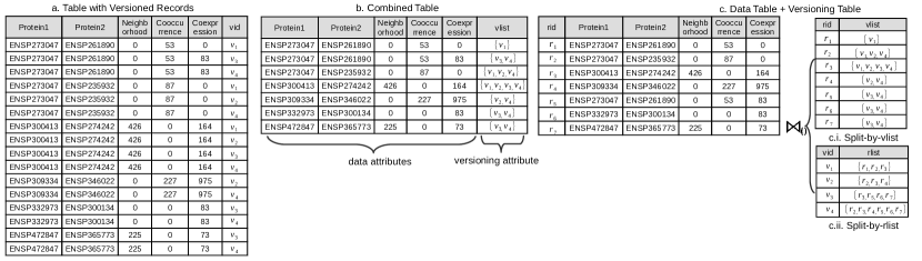
Figure 1: Data models for protein interaction data [48]

Challenges in Representation. One simple approach of capturing dataset versions would be to represent the dataset as a relation in a database, and add an extra attribute corresponding to the version number, called vid, as shown in Figure 1(a) for simplified protein-protein interaction data [48]; the other attributes will be introduced later. The version number attribute allows us to apply selection operations to retrieve specific versions. However, this approach is extremely wasteful as each record is repeated as many times as the number of versions it belongs to. It is worth noting that a timestamp is not sufficient here, as a version can have multiple parents (a merge) and multiple children (branches). Therefore, a scalar timestamp value cannot capture which versions a tuple belongs to. To remedy this issue, one can use the array data type capabilities offered in current database systems, by replacing the version number attribute with an array attribute vlist containing all of the versions that each record belongs to, as depicted in Figure 1(b). This reduces storage overhead from replicating tuples. However, when adding a new version (e.g., a clone of an existing version) this approach leads to extensive modifications across the entire relation, since the array will need to be updated for every single record that belongs to the new version. Another strategy is to separate the data from the versioning information into two tables as in Figure 1(c), where the first table—the data table—stores the records appearing in any of the versions, while the second table—the versioning table—captures the versioning information, or which version contains which records. This strategy requires us to perform a join of these two tables to retrieve any versions. Further, there are two ways of recording the versioning information: the first involves using an array of versions, the second involves using an array of records; we illustrate this in Figure 1(c.i) and Figure 1(c.ii) respectively. The latter approach allows easy insertion of new versions, without having to modify existing version information, but may have slight overheads relative to the former approach when it comes to joining the versioning table and the data table. Overall, as we demonstrate in this paper, the latter approach outperforms other approaches (including those based on recording deltas) for most common operations.

Challenges in Balancing Storage and Querying Latencies. Unfortunately, the previous approach still requires a full theta join and examination of all of the data to reconstruct any given version. Our next question is if we can improve the efficiency of the aforementioned approach, at the cost of possibly additional storage. One approach is to partition the versioning and data tables such that we limit data access to recreate versions, while keeping storage costs bounded. However, as we demonstrate in this paper, the problem of identifying the optimal trade-off between the storage and version retrieval time is NP-Hard, via a reduction from the 3-Partition problem. To address this issue, we develop an efficient and light-weight approximation algorithm, LyreSplit, that enables us to trade-off storage and version retrieval time, providing a guaranteed $((1+\delta)^{\ell},\frac{1}{\delta})$-factor approximation under certain reasonable assumptions—where the storage is a $(1+\delta)^{\ell}$-factor of optimal, and the average version retrieval time is $\frac{1}{\delta}$-factor of optimal, for any value of parameter $\delta\leq 1$ that expresses the desired trade-off. The parameter $\ell$ depends on the complexity of the branching structure of the version graph. In practice, this algorithm always leads to lower retrieval times for a given storage budget, than other schemes for partitioning, while being about $1000\times$ faster than these schemes. Further, we adapt LyreSplit to an online setting that incrementally maintains partitions as new versions arrive, and develop an intelligent migration approach to minimize the time taken for migration (by up to $10\times$).

Contributions. The contributions of this paper are as follows:

• We develop a dataset version control system, titled OrpheusDB, with the ability to support both git-style version control commands and SQL-like queries. (Section 2)

• We compare different data models for representing versioned datasets and evaluate their performance in terms of storage consumption and time taken for querying. (Section 3)

• To further improve query efficiency, we formally develop the optimization problem of trading-off between the storage and version retrieval time via partitioning and demonstrate that this is NP-Hard. We then propose a light-weight approximation algorithm for this optimization problem, titled LyreSplit, providing a $((1+\delta)^{\ell},\frac{1}{\delta})$-factor guarantee. (Section 4.2 and 4.1)

• We further adapt LyreSplit to be applicable to an online setting with new versions coming in, and develop an intelligent migration approach. (Section 4.3)

• We conduct extensive experiments using a versioning benchmark [37] and demonstrate that LyreSplit is on average 1000$\times$ faster than competing algorithms and performs better in balancing the storage and version retrieval time. We also demonstrate that our intelligent migration scheme reduces the migration time by $10\times$ on average. (Section 5)

2 OrpheusDB Overview

OrpheusDB is a dataset version management system that is built on top of standard relational databases. It inherits much of the same benefits of relational databases, while also compactly storing, tracking, and recreating versions on demand. OrpheusDB has been developed as open-source software (orpheus-db.github.io). We now describe fundamental version-control concepts, followed by the OrpheusDB APIs, and finally, the design of OrpheusDB.

2.1 Dataset Version Control

The fundamental unit of storage within OrpheusDB is a collaborative versioned dataset (cvd) to which one or more users can contribute. Each cvd corresponds to a relation and implicitly contains many versions of that relation. A version is an instance of the relation, specified by the user and containing a set of records. Versions within a cvd are related to each other via a version graph—a directed acyclic graph—representing how the versions were derived from each other: a version in this graph with two or more parents is defined to be a merged version. Records in a cvd are immutable, i.e., any modifications to any record attributes result in a new record, and are stored and treated separately within the cvd. Overall, there is a many-to-many relationship between records and versions: each record can belong to many versions, and each version can contain many records. Each version has a unique version id, vid, and each record has its unique record id, rid. The record ids are used to identify immutable records within the cvd and are not visible to end-users of OrpheusDB. In addition, the relation corresponding to the cvd may have primary key attribute(s); this implies that for any version no two records can have the same values for the primary key attribute(s). However, across versions, this need not be the case. OrpheusDB can support multiple cvds at a time. However, in order to better convey the core ideas of OrpheusDB, in the rest of the paper, we focus our discussion on a single cvd.

2.2 OrpheusDB APIs

Users interact with OrpheusDB via the command line, using both SQL queries, as well as git-style version control commands. In our companion demo paper, we also describe an interactive user interface depicting the version graph, for users to easily explore and operate on dataset versions [51]. To make modifications to versions, users can either use SQL operations issued to the relational database that OrpheusDB is built on top of, or can alternatively operate on them using programming or scripting languages. We begin by describing the version control commands.

Version control commands. Users can operate on cvds much like they would with source code version control. The first operation is checkout: this command materializes a specific version of a cvd as a newly created regular table within a relational database that OrpheusDB is connected to. The table name is specified within the checkout command, as follows:

$${\sf checkout~{}~{}[{\sc cvd}]~{}~{}\text{-}v~{}[vid]~{}~{}\text{-}t~{}[table~{}name]}\vspace{-5pt}$$

Here, the version with id vid is materialized as a new table [table name] within the database, to which standard SQL statements can be issued, and which can later be added to the cvd as a new version. The version from which this table was derived (i.e., vid) is referred to as the parent version for the table.

Instead of materializing one version at a time, users can materialize multiple versions, by listing multiple vids in the command above, essentially merging multiple versions to give a single table. When merging, the records in the versions are added to the table in the precedence order listed after -v: for any record being added, if another record with the same primary key has already been added, it is omitted from the table. This ensures that the eventual materialized table also respects the primary key property. There are other conflict-resolution strategies, such as letting users resolve conflicted records manually; for simplicity, we use a precedence based approach. Internally, the checkout command records the versions that this table was derived from (i.e., those listed after -v), along with the table name. Note that only the user who performed the checkout operation is permitted access to the materialized table, so they can perform any analysis and modification on this table without interference from other users, only making these modifications visible when they use the commit operation, described next.

The commit operation adds a new version to the cvd, by making the local changes made by the user on their materialized table visible to others. The commit command has the following format:

$${\sf commit~{}~{}\text{-}t~{}[table~{}name]~{}~{}\text{-}m~{}[commit~{}message]}\vspace{-5pt}$$

The command does not need to specify the intended cvd since OrpheusDB internally maintains a mapping between the table name and the original cvd. In addition, since the versions that the table was derived from originally during checkout are internally known to OrpheusDB, the table is added to the cvd as a new version with those versions as parent versions. During the commit operation, OrpheusDB checks the primary key constraint if PK is specified, and compares the (possibly) modified materialized table to the parent versions. If any records were added or modified these records are treated as new records and added to the cvd. (Recall that records are immutable within a cvd.) An alternative is to compare the new records with all of the existing records in the cvd to check if any of the new records have existed in any version in the past, which would take longer to execute. At the same time, the latter approach would identify records that were deleted then re-added later. Since we believe that this is not a common case, we opt for the former approach, which would only lead to modest additional storage at the cost of much less computation during commit. We call this the no cross-version diff implementation rule. Lastly, if the schema of the table that is being committed is different from the cvd it derived from, we alter the cvd to incorporate the new schema; we discuss this in Section 3.3, but for most of the paper we consider the static schema case.

In order to support data science workflows, we additionally support the use of checkout and commit into and from csv (comma separated value) files via slightly different flags: -f for csv instead of -t. The csv file can be processed in external tools and programming languages such as Python or R, not requiring that users perform the modifications and analysis using SQL. However, during commit, the user is expected to also provide a schema file via a -s flag so that OrpheusDB can make sure that the columns are mapped in the correct manner. An alternative would be to use schema inference tools, e.g., [38, 22], which could be seamlessly incorporated if need be. Internally, OrpheusDB also tracks the name of the csv file as being derived from one or more versions of the cvd, just like it does with the materialized tables.

In addition to checkout and commit, OrpheusDB also supports other commands, described very briefly here: (a) diff:a standard differencing operation that compares two versions and outputs the records in one but not the other. (b) init:initialize either an external csv file or a database table as a new cvd in OrpheusDB. (c) create_user, config, whoami:allows users to register, login, and view the current user name. (d) ls, drop: list all the cvds or drop a particular cvd. (e) optimize:as we will see later, OrpheusDB can benefit from intelligent incremental partitioning schemes (enabling operations to process much less data). Users can setup the corresponding parameters (e.g., storage threshold, tolerance factor, described later) via the command line; the OrpheusDB backend will periodically invoke the partitioning optimizer to improve the versioning performance.

SQL commands. OrpheusDB supports the use of SQL commands on cvds via the command line using the run command, which either takes a SQL script as input or the SQL statement as a string. Instead of materializing a version (or versions) as a table via the checkout command and explicitly applying SQL operations on that table, OrpheusDB also allows users to directly execute SQL queries on a specific version, using special keywords VERSION, OF, and CVD via syntax

SELECT … FROM VERSION [vid] OF CVD [cvd], …

without having to materialize it. Further, by using renaming, users can operate directly on multiple versions (each as a relation) within a single SQL statement, enabling operations such as joins across multiple versions.

However, listing each version individually as described above may be cumbersome for some types of queries that users wish to run, e.g., applying an aggregate across a collection of versions, or identifying versions that satisfy some property. For this, OrpheusDB also supports constructs that enable users to issue aggregate queries across cvds grouped by version ids, or select version ids that satisfy certain constraints. Internally, these constructs are translated into regular SQL queries that can be executed by the underlying database system. In addition, OrpheusDB provides shortcuts for several types of queries that operate on the version graph, e.g., listing the descendant or ancestors of a specific version, or querying the metadata, e.g., identify the last modification (in time) to the cvd. The details of the query syntax, translation, as well as examples can be found in our companion demo paper [51].

2.3 System Architecture

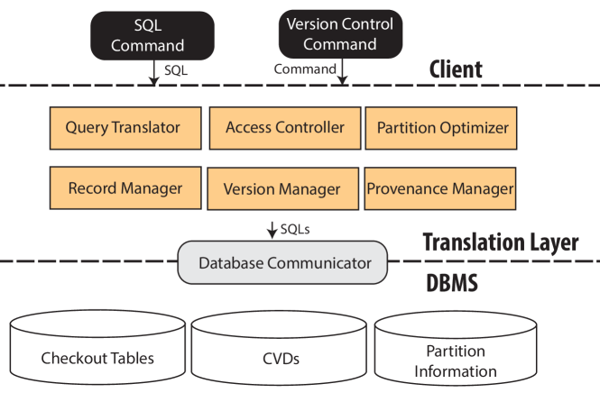
Figure 2: OrpheusDB Architecture

We implement OrpheusDB as a middleware layer or wrapper between end-users (or application programs) and a traditional relational database system—in our case, PostgreSQL. PostgreSQL is completely unaware of the existence of versioning, as versioning is handled entirely within the middleware. Figure 2 depicts the overall architecture of OrpheusDB. OrpheusDB consists of six core modules: the query translator is responsible for parsing input and translating it into SQL statements understandable by the underlying database system; the access controller monitors user permissions to various tables and files within OrpheusDB; the partition optimizer is responsible for periodically reorganizing and optimizing the partitions via a partitioning algorithm LyreSplit along with a migration engine to migrate data from one partitioning scheme to another, and is the focus of Section 4; the record manager is in charge of recording and retrieving information about records in cvds; the version manager is in charge of recording and retrieving versioning information, including the rids each version contains as well as the metadata for each version; and the provenance manager is responsible for the metadata of uncommitted tables or files, such as their parent version(s) and the creation time. At the backend, a traditional DBMS, we maintain cvds that consist of versions, along with the records they contain, as well as metadata about versions. In addition, the underlying DBMS contains a temporary staging area consisting of all of the materialized tables that users can directly manipulate via SQL without going through OrpheusDB. Understanding how to best represent and operate on these cvds within the underlying DBMS is an important challenge—this is the focus of the next section.

In brief, we now describe how these components work with each other for the basic checkout and commit commands, once the command is parsed. For checkout, the query translator generates SQL queries to retrieve records from the relevant versions, which are then handled and materialized in the temporary staging area by the record manager; the provenance manager logs the related derivation information and other metadata; and finally the access controller to grant permissions to the relevant user. On commit, the record manager appends new records to the cvd, also performs cleanup by removing the table from the staging area; the version manager updates the metadata of the newly added version.

Command	SQL Translation with combined-table	SQL Translation with Split-by-vlist	SQL Translation with Split-by-rlist
CHECKOUT	SELECT * into T’ FROM T WHERE ARRAY[$v_{i}$] <@ vlist	SELECT * into T’ FROM dataTable, (SELECT rid AS rid_tmp FROM versioningTable WHERE ARRAY[$v_{i}$] <@ vlist) AS tmp WHERE rid = rid_tmp	SELECT * into T’ FROM dataTable, (SELECT unnest(rlist) AS rid_tmp FROM versioningTable WHERE vid = $v_{i}$) AS tmp WHERE rid = rid_tmp
COMMIT	UPDATE T SET vlist=vlist+$v_{j}$ WHERE rid in (SELECT rid FROM T’)	UPDATE versioningTable SET vlist=vlist+$v_{j}$ WHERE rid in (SELECT rid FROM T’)	INSERT INTO versioningTable VALUES ($v_{j}$, ARRAY[SELECT rid FROM T’])

Table 1: SQL Queries for Checkout and Commit Commands with Different Data Models

3 Data Models for cvds

In this section, we consider and compare methods to represent and operate on cvds within a backend relational database, starting with the data within versions, and then the metadata about versions.

3.1 Versions and Data: The Models

To explore alternative storage models, we consider the array-based data models, shown in Figure 1, and compare them to a delta-based data model, which we describe later. The table(s) in Figure 1 displays simplified protein-protein interaction data [48], and has a composite primary key <protein1, protein2>, along with numerical attributes indicating sources and strength of interactions: neighborhood represents how frequently the two proteins occur close to each other in runs of genes, cooccurrence reflects how often the two proteins co-occur in the species, and coexpression refers to the level to which genes are co-expressed in the species.

One approach, as described in the introduction, is to augment the cvd’s relational schema with an additional versioning attribute. For example, in Figure 1(a) the tuple of <ENSP273047, ENSP261890, 0, 53, 83> exists in two versions: $v_{3}$ and $v_{4}$. (Note that even though <protein1, protein2> is the primary key, it is only the primary key for any single version and not across all versions.) There are two records with <ENSP273047, ENSP261890> that have different values for the other attributes: one with (0, 53, 83) that is present in $v_{3}$ and $v_{4}$, and another with (0, 53, 0) that is present in $v_{1}$. However, this approach implies that we would need to duplicate each record as many times as the number of versions it is in, leading to severe storage overhead due to redundancy, as well as inefficiency for several operations, including checkout and commit. We focus on alternative approaches that are more space efficient and discuss how they can support the two most fundamental operations—commit and checkout—on a single version at a time. Considerations for multiple version checkout is similar to that for a single version; our findings generalize to that case as well.

Approach 1: The Combined Table Approach. Our first approach of representing the data and versioning information for a cvd is the combined table approach. As before, we augment the schema with an additional versioning attribute, but now, the versioning attribute is of type array and is named vlist (short for version list) as shown in Figure 1(b). For each record the vlist is the ordered list of version ids that the record is present in, which serves as an inverted index for each record. Returning to our example, there are two versions of records corresponding to <ENSP273047, ENSP261890>, with coexpression 0 and 83 respectively—these two versions are depicted as the first two records, with an array corresponding to $v_{1}$ for the first record, and $v_{3}$ and $v_{4}$ for the second.

Even though array is a non-atomic data type, it is commonly supported in many database systems [8, 3, 1]; thus OrpheusDB can be built with any of these systems as the back-end database. As our implementation uses PostgreSQL, we focus on this system for the rest of the discussion, even though similar considerations apply to the rest of the databases listed. PostgreSQL provides a number of useful functions and operators for manipulating arrays, including append operations, set operations, value containment operations, and sorting and counting functions.

For the combined table approach, committing a new version to the cvd is time-consuming due to the expensive append operation for every record present in the new version. Consider the scenario where the user checks out version $v_{i}$ into a materialized table $T^{\prime}$ and then immediately commits it back as a new version $v_{j}$. The query translator parses the user commands and generates the corresponding SQL queries for checkout and commit as shown in Table 1. In the checkout statement, the containment operator ‘int[] <@ int[]’ returns true if the array on the left is contained within the array on the right. When checking out $v_{i}$ into a materialized table $T^{\prime}$, the array containment operator ‘ARRAY[$v_{i}$] <@ vlist’ first examines whether $v_{i}$ is contained in vlist for each record in cvd, then all records that satisfy that condition are added to the materialized table $T^{\prime}$. Next, when $T^{\prime}$ is committed back to the cvd as a new version $v_{j}$, for each record in the cvd, if it is also present in $T^{\prime}$ (i.e., the WHERE clause), we append $v_{j}$ to the attribute vlist (i.e., vlist=vlist+$v_{j}$). In this case, since there are no new records that are added to the cvd, no new records are added to the combined table. However, even this process of appending $v_{j}$ to vlist can be expensive especially when the number of records in $v_{j}$ is large, as we will demonstrate.

Approach 2: The Split-by-vlist Approach. Our second approach addresses the limitations of the expensive commit operation for the combined table approach. We store two tables, keeping the versioning information separate from the data information, as depicted in Figure 1(c)—the data table and the versioning table. The data table contains all of the original data attributes along with an extra primary key rid, while the versioning table maintains the mapping between versions and rids. The rid attribute was not needed in the previous approach since it was not necessary to associate identifiers with the immutable records. Specifically, the relation primary key— <protein1, protein2> —is not sufficient to distinguish between multiple copies of the same record. For example, $r1$ and $r5$ are two versions of the same record (i.e., the record with a given <protein1, protein2>). There are two ways we can store the versioning data. The first approach is to store the rid along with the vlist, as depicted in Figure 1(c.i). We call this approach split-by-vlist. Split-by-vlist has a similar SQL translation as combined-table for commit, while it incurs the overhead of joining the data table with the versioning table for checkout. Specifically, we select the rids that are in the version to be checked out and store it in the table tmp, followed by a join with the data table. For example, when checking out version $v_{1}$, tmp will comprise the relevant rids $r_{1},r_{2},r_{3}$, which are identified by looking at the vlist for each record in the versioning table and checking if $v_{1}$ is present, which is then joined with the data table to extract the appropriate results into the materialized table $T^{\prime}$.

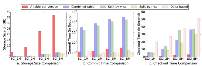
Figure 3: Comparison Between Different Data Models

Approach 3: The Split-by-rlist Approach. Alternatively, we can organize the versioning table with a primary key as vid (version id), and another attribute rlist, containing the array of the records present in that particular version, as in Figure 1(c.ii). We call this approach the split-by-rlist approach. When committing a new version $v_{j}$ from the materialized table $T^{\prime}$, we only need to add a single tuple in the versioning table with vid equal to $v_{j}$, and rlist equal to the list of record ids in $T^{\prime}$. This eliminates the expensive array appending operations that are part of the previous two approaches, making the commit command much more efficient. For the checkout command for version $v_{i}$, we first extract the record ids associated with $v_{i}$ from the versioning table, by applying the unnesting operation: unnest(rlist), following which we join the rids with the data table to identify all of the relevant records. For example, for checking out $v_{1}$, instead of examining the entire versioning table, we simply need to examine the tuple corresponding to $v_{1}$, unnest those rids—$r_{1},r_{2},r_{3}$, followed by a join.

So far, all our models support convenient rewriting of arbitrary and complex versioning queries into SQL queries understood by the backend database; see details in our demo paper [51]. However, our delta-based model, discussed next, does not support convenient rewritings for some of the more advanced queries, e.g., “find versions where the total count of tuples with protein1 as ENSP273047 is greater than 50”: in such cases, delta-based model essentially needs to recreate all of the versions, and/or perform extensive and expensive computation outside of the database. Thus, even though this model does not support advanced analytics capabilities “for free”, we include it in our comparison to contrast its performance to the array-based models.

Approach 4: Delta-based Approach. Here, each version records the modifications (or deltas) from its precedent version(s). Specifically, each version is stored as a separate table, with an added tombstone boolean attribute indicating the deletion of a record. In addition, we maintain a precedent metadata table with a primary key vid and an attribute base indicating from which version vid stores the delta. When committing a new version $v_{j}$, a new table stores the delta from its previous version $v_{i}$. If $v_{j}$ has multiple parents, we will store $v_{j}$ as the modification from the parent that shares the largest common number of records with $v_{j}$. (Storing deltas from multiple parents would make reconstruction of a version complicated, since we would need to trace back multiple paths in the version graph, or alternatively materialize each version in the version graph in a top-down manner, merging versions based on conflict resolution mechanisms. Here, we opt for the simpler solution.) A new record is then inserted into the metadata table, with vid as $v_{j}$ and base as $v_{i}$. For the checkout command for version $v_{i}$, we trace the version lineage (via the base attribute) all the way back to the root. If an incoming record has occurred before, it is discarded; otherwise, if it is marked as “insert”, we insert it into the checkout table $T^{\prime}$.

Approach 5: The A-Table-Per-Version Approach. Our final array-based data model is impractical due to excessive storage, but is useful from a comparison standpoint. In this approach, we store each version as a separate table. We include a-table-per-version in our comparison; we do not include the approach in Figure 1a, containing a table with duplicated records, since it would do similarly in terms of storage and commit times to a-table-per-version, but worse in terms of checkout times.

3.2 Versions and Data: The Comparison

We perform an experimental evaluation between the approaches described in the previous section on storage size, and commit and checkout time. We focus on the commit and checkout times since they are the primitive versioning operations on which the other more complex operations and queries are built on. It is important that these operations are efficient, because data scientists checkout a version to start working on it immediately, and often commit a version to have their changes visible to other data scientists who may be waiting for them.

In our evaluation, we use four versioning benchmark datasets SCI_1M, SCI_2M, SCI_5M and SCI_8M, each with $1M$, $2M$, $5M$ and $8M$ records respectively, that will be described in detail in Section 5.1. For split-by-vlist, a physical primary key index is built on rid in both the data table and the versioning table; for split-by-rlist, a physical primary key index is built on rid in the data table and on vid in the versioning table. When calculating the total storage size, we count the index size as well. Our experiment involves first checking out the latest version $v_{i}$ into a materialized table $T^{\prime}$ and then committing $T^{\prime}$ back into the cvd as a new version $v_{j}$. We depict the experimental results in Figure 3.

Storage. From Figure 3(a), we can see that a-table-per-version takes $10\times$ more storage than the other data models. This is because each record exists on average in 10 versions. Compared to a-table-per-version and combined-table, split-by-vlist and split-by-rlist deduplicate the common records across versions and therefore have roughly similar storage. In particular, split-by-vlist and split-by-rlist share the same data table, and thus the difference can be attributed to the difference in the size of the versioning table. For the delta-based approach, the storage size is similar to or even slightly smaller than split-by-vlist and split-by-rlist. This is because our versioning benchmark contains only a few deleted tuples (opting instead for updates or inserts); in other cases, where deleted tuples are more prevalent, the storage in the delta-based approach is worse than split-by-vlist/rlist, since the deleted records will be repeated. We also remark that the storage size for array-based appoaches can be further reduced by applying compression techniques like range-encoding [14].

Commit. From Figure 3(b), we can see that the combined-table and split-by-vlist take multiple orders of magnitude more time than split-by-rlist for commit. We also notice that the commit time when using combined-table is almost $10^{4}s$ as the dataset size increases: when using combined-table, we need to add $v_{j}$ to the attribute vlist for each record in the cvd that is also present in $T^{\prime}$. Similarly, for split-by-vlist, we need to perform an append operation for several tuples in the versioning table. On the contrary, when using split-by-rlist, we only need to add one tuple to the versioning table, thus getting rid of the expensive array appending operations. A-table-per-version also has higher latency for commit than split-by-rlist since it needs to insert all the records in $T^{\prime}$ into the cvd. For the delta-based approach, the commit time is small since the new version $v_{j}$ is exactly the same as its precedent version $v_{i}$. It only needs to update the precedent metadata table, and create a new empty table. The commit time of the delta-based approach is not small in general when there are extensive modifications to $T^{\prime}$, as illustrated by other experiments (not displayed); For instance, for a committed version with 250K records of which 30% of the records are modified, delta-based takes 8.16s, while split-by-rlist takes 4.12s.

Checkout. From Figure 3 (c), we can see that split-by-rlist is a bit faster than combined-table and split-by-vlist for checkout. Not surprisingly, a-table-per-version is the best for this operation since it simply requires retrieving all the records in a specific table (corresponding to the desired version). We dive into the query plan for the other data models. Combined-table requires one full scan over the combined table to check whether each record is in version $v_{i}$. On the other hand, split-by-vlist needs to first scan the versioning table to retrieve the rids in version $v_{i}$, and then join the rids with the data table. Lastly, split-by-rlist retrieves the rids in version $v_{i}$ using the primary key index on vid in the versioning table, and then joins the rids with the data table. For both split-by-vlist and split-by-rlist, we used a hash-join, which was the most efficient, where a hash table on rids is first built, followed by a sequential scan on the data table by probing each record in the hash table. Overall, combined-table, split-by-vlist, and split-by-rlist all require a full scan on the combined table or the data table, and even though split-by-rlist introduces the overhead of building a hash table, it reduces the expensive array operation for containment checking as in combined-table and split-by-vlist. For the delta-based approach, the checkout time is large since it needs to probe into a number of tables, tracing all the way back to the root, remembering which records were seen.

Takeaways. Overall, considering the space consumption, the commit and checkout time, plus the fact that delta-based models are inefficient in supporting advanced queries as discussed in Section 3.1, we claim that split-by-rlist is preferable to the other data models in supporting versioning within a relational database. Thus, we pick split-by-rlist as our data model for representing cvds. That said, from Figure 3(c), we notice that the checkout time for split-by-rlist grows with dataset size. For instance, for dataset SCI_8M with $8M$ records in the data table, the checkout time is as high as 30 seconds. On the other hand, a-table-per-version has very low checkout times on all datasets; it only needs to access the relevant records instead of all records as in split-by-rlist. This motivates the need for the partition optimizer module in OrpheusDB, which tries to attain the best of both worlds by adopting a hybrid representation of split-by-rlist and a-table-per-version, described in Section 4.

3.3 Version Derivation Metadata

Version Provenance. As discussed in Section 2.3, the version manager in OrpheusDB keeps track of the derivation relationships among versions and maintains metadata for each version. We store version-level provenance information in a separate table called the metadata table; Figure 4(a) depicts the metadata table for the example in Figure 1. It contains attributes including version id, parent/child versions, creation time, commit time, a commit message, and an array of attributes present in the version. Using the data contained in this table, users can easily query for the provenance of versions and for other metadata. In addition, using the attribute parents we can obtain each version’s derivation information and visualize it as directed acyclic graph that we call a version graph. Each node in the version graph is a version and each directed edge points from a version to one of its children version(s). An example is depicted in Figure 4(b), where version $v_{2}$ and $v_{3}$ are both derived from version $v_{1}$, and version $v_{2}$ and $v_{3}$ are merged into version $v_{4}$. We will return to this concept in Section 4.2.

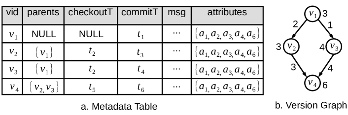
Figure 4: Metadata Table and Version Graph (Fixed Schema)

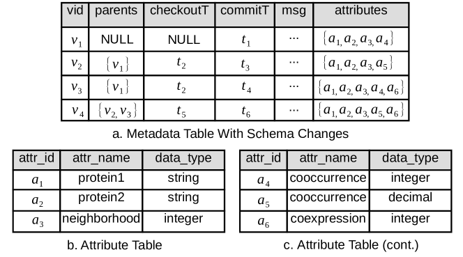
Figure 5: Metadata Table and Attribute Table (Schema Changes)

Schema Changes. During a commit, if the schema of the table being committed is different from the schema of the cvd it was derived from, we update the schema of cvd to incorporate the changes. More precisely, in OrpheusDB, we maintain an attribute table (as in Figure 5) where each tuple represents an attribute with a unique identifier, along with the corresponding attribute name and data type; any change of a property of an attribute results in a new attribute entry in the table. If the data type of any attribute changes, we transform the attribute type to a more general data type (e.g., from integer to string as in Jain et al. [24]), and insert a new tuple into the attribute table with the updated data type. All of our array-based models can adapt to changes in the set of attributes: a simple solution for new attributes is so use the ALTER command to add any new attributes to the model, assigning NULLs to the records from the previous versions that do not possess these new attributes. Attribute deletions only require an update in the version metadata table. To illustrate, we modify the previous example in Figure 4 (which showed a static schema) to a dynamic one. For example, as shown in Figure 5, initially version $v_{1}$ has four attributes: protein1, protein2, neighborhood and cooccurrence. When a user commits version $v_{2}$, with the data type of the cooccurrence attribute ($a_{4}$) changed from integer to decimal, within OrpheusDB, we create another attribute ($a_{5}$) in the attribute table with data type decimal, log $a_{5}$ in the metadata table for $v_{2}$ and alter the cooccurrence attribute to decimal within the cvd. Moreover, when a new coexpression attribute is added in $v_{3}$, we generate a corresponding attribute ($a_{6}$) in the attribute table, add $a_{6}$ in the metadata table for $v_{3}$, and add the coexpression attribute to the cvd. During the merge, the resulting version includes all attributes from its parents and contains the more general data type for conflicting attributes (e.g., attributes in $v_{4}$). This simple mechanism is similar to the single pool method proposed in a temporal schema versioning context by De Castro et al. [18]. Compared to the multi pool method where any schema change results in the new version being stored separately, the single pool method has fewer records with duplicated attributes and therefore has less storage consumption overall. Even though ALTER TABLE is indeed a costly operation, due to the partitioning schemes we describe later, we only need to ALTER a smaller partition of the cvd rather than a giant cvd, and consequently the cost of an ALTER operation is substantially mitigated. In Appendix C.3, we describe how our partitioning schemes (described next in Section 4) can adapt to the single pool mechanism with comparable guarantees; for ease of exposition, for the rest of this paper, we focus on the static schema case, which is still important and challenging. There has been some work on developing schema versioning schemes [19, 40, 39] and we plan to explore these and other schema evolution mechanisms (including hybrid single/multi-pool methods) as future work.

4 Partition Optimizer

Recall that Figure 3(c) indicated that as the number of records within a cvd increases, the checkout latency of our data model (split-by-rlist) increases—this is because the number of “irrelevant” records, i.e., the records that are not present in the version being checked out, but nevertheless require processing increases. Even with index on rid, the checkout latency is still high since records are scattered across the whole data table, and hundreds of thousands of random accesses are eventually reduced to a full table scan as demonstrated in Appendix D.1. In this section, we introduce the concept of partitioning a cvd by breaking up the data and versioning tables, in order to reduce the number of irrelevant records during checkout. We formally define our partitioning problem, demonstrate that this problem is NP-Hard, and identify a light-weight approximation algorithm. We provide a convenient table of notation in the Appendix (Table 3).

4.1 Problem Overview

The Partitioning Notion. Let $V=\{v_{1},v_{2},...,v_{n}\}$ be the $n$ versions and $R=\{r_{1},r_{2},...,$ $r_{m}\}$ be the $m$ records in a cvd. We can represent the presence of records in versions using a version-record bipartite graph $G=(V,R,E)$, where $E$ is the set of edges—an edge between $v_{i}$ and $r_{j}$ exists if the version $v_{i}$ contains the record $r_{j}$. The bipartite graph in Figure 6(a) captures the relationships between records and versions in Figure 1.

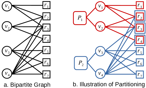
Figure 6: Version-Record Bipartite Graph & Partitioning

The goal of our partitioning problem is to partition $G$ into smaller subgraphs, denoted as $\mathcal{P}_{k}$. We let $\mathcal{P}_{k}=(\mathcal{V}_{k},\mathcal{R}_{k},\mathcal{E}_{k})$, where $\mathcal{V}_{k}$, $\mathcal{R}_{k}$ and $\mathcal{E}_{k}$ represent the set of versions, records and bipartite graph edges in partition $\mathcal{P}_{k}$ respectively. Note that $\cup_{k}\mathcal{E}_{k}=E$, where $E$ is the set of edges in the original version-record bipartite graph $G$. We further constrain each version in the cvd to exist in only one partition, while each record can be duplicated across multiple partitions. In this manner, we only need to access one partition when checking out a version, consequently simplifying the checkout process by reducing the overhead from accessing multiple partitions. (While we do not consider it in this paper, in a distributed setting, it is even more important to ensure that as few partitions are consulted during a checkout operation.) Thus, our partition problem is equivalent to partitioning $V$, such that each partition ($\mathcal{P}_{k}$) stores all of the records corresponding to all of the versions assigned to that partition. Figure 6(b) illustrates a possible partitioning strategy for Figure 6(a). Partition $\mathcal{P}_{1}$ contains version $v_{1}$ and $v_{2}$, while partition $\mathcal{P}_{2}$ contains version $v_{3}$ and $v_{4}$. Note that records $r_{2},r_{3}$ and $r_{4}$ are duplicated in $\mathcal{P}_{1}$ and $\mathcal{P}_{2}$.

Metrics. We consider two criteria while partitioning: the storage cost and the time for checkout. Recall that the time for commit is fixed and small—see Figure 3(b), so we only focus on checkout.

The overall storage costs involves the cost of storing all of the partitions of the data and the versioning table. However, we observe that the versioning table simply encodes the bipartite graph, and as a result, its cost is fixed. Furthermore, since all of the records in the data table have the same (fixed) number of attributes, so instead of optimizing the actual storage we will optimize for the number of records in the data table across all the partitions. Thus, we define the storage cost, $\mathcal{S}$, to be the following:

$$\small\mathcal{S}=\sum_{k=1}^{K}|\mathcal{R}_{k}|$$ (4.1)

Next, we note that the time taken for checking out version $v_{i}$ is proportional to the size of the data table in the partition $\mathcal{P}_{k}$ that contains version $v_{i}$, which in turn is proportional to the number of records present in that data table partition. We theoretically and empirically justify this in Appendix D.1. So we define the checkout cost of a version $v_{i}$, $\mathcal{C}_{i}$, to be $\mathcal{C}_{i}=|\mathcal{R}_{k}|$, where $v_{i}\in\mathcal{V}_{k}$. The checkout cost, denoted as $\mathcal{C}_{avg}$, is defined to be the average of $\mathcal{C}_{i}$, i.e., $\mathcal{C}_{avg}=\frac{\sum_{i}\mathcal{C}_{i}}{n}$. While we focus on the average case, which assumes that each version is checked out with equal frequency—a reasonable assumption when we have no other information about the workload, our algorithms generalize to the weighted case as described in Appendix C.2. (The weighted case can help represent the workload in real world settings, where recent versions may be checked out more frequently.) On rewriting the expression for $\mathcal{C}_{avg}$ above, we get:

$$\small\mathcal{C}_{avg}=\frac{\sum_{k=1}^{K}|\mathcal{V}_{k}||\mathcal{R}_{k}|}{n}\vspace{4mm}$$ (4.2)

The numerator is simply sum of the number of records in each partition, multiplied by the number of versions in that partition, across all partitions—this is the cost of checking out all of the versions.

Formal Problem. Our two metrics $\mathcal{S}$ and $\mathcal{C}_{avg}$ interfere with each other: if we want a small $\mathcal{C}_{avg}$, then we need more storage, and if we want the storage to be small, then $\mathcal{C}_{avg}$ will be large. Typically, storage is under our control; thus, our problem can be stated as:

Problem 1 (Minimize Checkout Cost)

Given a storage threshold $\gamma$ and a version-record bipartite graph $G=(V,R,E)$, find a partitioning of $G$ that minimizes $\mathcal{C}_{avg}$ such that $\mathcal{S}\leq\gamma$.

We can show that Problem 1 is NP-Hard using a reduction from the 3-Partition problem, whose goal is to decide whether a given set of $n$ integers can be partitioned into $\frac{n}{3}$ sets with equal sum. 3-Partition is known to be strongly NP-Hard, i.e., it is NP-Hard even when its numerical parameters are bounded by a polynomial in the length of the input.

Theorem 1

Problem 1 is NP-hard.

The proof for this theorem can be found in Appendix A.

We now clarify one complication between our formalization so far and our implementation. OrpheusDB uses the no cross-version diff rule: that is, while performing a commit operation, to minimize computation, OrpheusDB does not compare the committed version against all of the ancestor versions, instead only comparing it to its parents. Therefore, if some records are deleted and then re-added later, these records would be assigned different rids, and are treated as different. As it turns out, Problem 1 is still NP-Hard when the space of instances are those that can be generated when this rule is applied. For the rest of this section, we will use the formalization with the no cross-version diff rule in place, since that relates more closely to practice.

4.2 Partitioning Algorithm

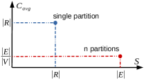
Figure 7: Extreme Schemes

Given a version-record bipartite graph $G=(V,R,E)$, there are two extreme cases for partitioning. At one extreme, we can minimize the checkout cost by storing each version in the cvd as one partition; there are in total $K=|V|=n$ partitions, and the storage cost is $\mathcal{S}=\sum_{k=1}^{n}|\mathcal{R}_{k}|=|E|$ and the checkout cost is $\mathcal{C}_{avg}=\frac{1}{n}\sum_{k=1}^{n}$ $(|\mathcal{V}_{k}||\mathcal{R}_{k}|)=\frac{|E|}{|V|}$. At another extreme, we can minimize the storage by storing all versions in one single partition; the storage cost is $\mathcal{S}=|R|$ and $\mathcal{C}_{avg}=|R|$. We illustrate these schemes in Figure 7. We also list them as formal observations below:

Observation 1

Given a bipartite graph $G=(V,R,E)$, the checkout cost $\mathcal{C}_{avg}$ is minimized by storing each version as one separate partition: $\mathcal{C}_{avg}=\frac{|E|}{|V|}$.

Observation 2

Given a bipartite graph $G=(V,R,E)$, the storage cost $\mathcal{S}$ is minimized by storing all versions in a single partition: $\mathcal{S}=|R|$.

Version Graph Concept. Our goal in designing our partitioning algorithm, LyreSplit , is to trade-off between these two extremes. Instead of operating on the version-record bipartite graph, which may be very large, LyreSplit operates on the much smaller version graph instead, which makes it a lot more lightweight. We recall the concept of a version graph from Section 3.3, and depicted in Figure 4. We denote a version graph as $\mathbb{G}=(\mathbb{V},\mathbb{E})$, where each vertex $v\in\mathbb{V}$ is a version and each edge $e\in\mathbb{E}$ is a derivation relationship. Note that $\mathbb{V}$ is essentially the same as $V$ in the version-record bipartite graph. An edge from vertex $v_{i}$ to a vertex $v_{j}$ indicates that $v_{i}$ is a parent of $v_{j}$; this edge has a weight $w(v_{i},v_{j})$ equals the number of records in common between $v_{i}$ and $v_{j}$. We use $p(v_{i})$ to denote the parent versions of $v_{i}$. For the special case when there are no merge operations, $|p(v_{i})|\leq 1,\forall i$, and the version graph is a tree, denoted as $\mathbb{T}=(\mathbb{V},\mathbb{E})$. Lastly, we use $R(v_{i})$ to be the set of all records in version $v_{i}$, and $l(v_{i})$ to be the depth of $v_{i}$ in the version graph $\mathbb{G}$ in a topological sort of the graph—the root has depth 1. For example, in Figure 4, version $v_{2}$ has $|R(v_{2})|=3$ since it has three records, and is at level $l(v_{2})=2$. Further, $v_{2}$ has a single parent $p(v_{2})=v_{1}$, and shares two records with its parent, i.e., $w(v_{1},v_{2})=2$. Next, we describe the algorithm for LyreSplit when the version graph is a tree (i.e., no merge operations). We then naturally extend our algorithm to other settings, as we will describe next.

The Version Tree Case. Our algorithm is based on the following lemma, which intuitively states that if every version $v_{i}$ shares a large number of records with its parent version, then the checkout cost is small, and bounded by some factor of $\frac{|E|}{|V|}$, where $\frac{|E|}{|V|}$ is the lower bound on the optimal checkout cost (from Observation 1).

Lemma 1

Given a bipartite graph $G=(V,R,E)$, a version tree $\mathbb{T}=(\mathbb{V},\mathbb{E})$, and a parameter $\delta\leq 1$, if the weight of every edge in $\mathbb{E}$ is larger than $\delta|R|$, then the checkout cost $\mathcal{C}_{avg}$ when all of the versions are in one single partition is less than $\frac{1}{\delta}\cdot\frac{|E|}{|V|}$.

Proof 4.2.

Consider the nodes of the version tree $\mathbb{T}$ level-by-level, starting from the root. That is, all of a version’s ancestors are considered before it is evaluated. Now, given a version $v_{i}$, the number of new records added by $v_{i}$ is $R(v_{i})-w(v_{i},p(v_{i}))$. Thus, we have:

$$\small\begin{split}|R|&=|\cup_{i=1}^{|V|}R(v_{i})|\\ &=R(v_{1})+\sum_{l(v_{i})=2}(R(v_{i})-w(v_{i},p(v_{i})))\\ &+\sum_{l(v_{i})=3}(R(v_{i})-w(v_{i},p(v_{i})))+\cdots\\ \implies|R|&=\sum_{i=1}^{|V|}R(v_{i})-\sum_{i=2}^{|V|}(w(v_{i},p(v_{i})))\\ \end{split}$$

Since each edge weight is larger than $\delta|R|$, i.e., $w(v_{i},p(v_{i}))>\delta|R|,\forall 2\leq i\leq|V|$, we have:

$$|R|<|E|-\delta(|V|-1)|R|\leq|E|-\delta|V||R|+|R|$$

where the last inequality is because $\delta\leq 1$. Thus, we have $|R|<\frac{1}{\delta}\cdot\frac{|E|}{|V|}$. Since $\mathcal{C}_{avg}=|R|$ when we have only one partition, the result follows.

Lemma 1 indicates that when $\mathcal{C}_{avg}\geq\frac{1}{\delta}\cdot\frac{|E|}{|V|}$, there must exist some version $v_{j}$ that only shares a small number of common records with its parent version $v_{i}$, i.e., $w(v_{i},v_{j})\leq\delta|R|$; otherwise $\mathcal{C}_{avg}<\frac{1}{\delta}\cdot\frac{|E|}{|V|}$. Intuitively, such an edge $(v_{i},v_{j})$ with $w(v_{i},v_{j})\leq\delta|R|$ is a potential edge for splitting since the overlap between $v_{i}$ and $v_{j}$ is small.

Input : Version tree $\mathbb{G}=(\mathbb{V},\mathbb{E})$ and parameter $\delta$

Output : Partitions $\{\mathcal{P}_{1},\mathcal{P}_{2},\cdots,\mathcal{P}_{K}\}$

1 if $|R|\times|V|<\frac{|E|}{\delta}$ then

2       return $V$

3 end if

4else

5       $\Omega\leftarrow\{e|e.w\leq\delta\times|R|,e\in\mathbb{E}\}$

6       $e^{*}\leftarrow\text{PickOneEdgeCut}(\Omega)$

7       Remove $e^{*}$ and split $\mathbb{G}$ into two parts $\{\mathbb{G}_{1},\mathbb{G}_{2}\}$

8       Update the number of records, versions and bipartite edges in $\mathbb{G}_{1}$, denoted as $|R_{1}|$, $|V_{1}|$ and $|E_{1}|$

9       Update the number of records, versions and bipartite edges in $\mathbb{G}_{2}$, denoted as $|R_{2}|$, $|V_{2}|$ and $|E_{2}|$

10       $\mathcal{P}_{1}$=LyreSplit ($\mathbb{G}_{1},|R_{1}|,|V_{1}|,|E_{1}|,\delta$)

11       $\mathcal{P}_{2}$=LyreSplit ($\mathbb{G}_{2},|R_{2}|,|V_{2}|,|E_{2}|,\delta$)

12       return $\{\mathcal{P}_{1},\mathcal{P}_{2}\}$

13 end if

Algorithm 1 LyreSplit ($\mathbb{G},|R|,|V|,|E|,\delta$)

LyreSplit Illustration. We describe a version of LyreSplit that accepts as input a parameter $\delta$, and then recursively applies partitioning until the overall $\mathcal{C}_{avg}<\frac{1}{\delta}\cdot\frac{|E|}{|V|}$; we will adapt this to Problem 1 later. The pseudocode is provided in Algorithm 1, and we illustrate its execution on an example in Figure 8.

As before, we are given a version tree $\mathbb{T}=(\mathbb{V},\mathbb{E})$. We start with all of the versions in one partition. We first check whether $|R||V|<\frac{|E|}{\delta}$ (line 1). If yes, then we terminate; otherwise, we pick one edge $e^{*}$ with weight $e^{*}.w\leq\delta|R|$ (lines 5–6) to cut in order to split the partition into two. According to Lemma 1, if $|R||V|\geq\frac{|E|}{\delta}$, there must exist some edge whose weight is no larger than $\delta|R|$. The algorithm does not prescribe a method for picking this edge if there are multiple; the guarantees hold independent of this method. For instance, we can pick the edge with the smallest weight; or the one such that after splitting, the difference in the number of versions in the two partitions is minimized. In our experiments, we use the latter, and break a tie by selecting the edge that balances the records between two partitions in addition to the number of versions. In our example in Figure 8(a), we first find that having the entire version tree as a single partition violates the property, and we pick the red edge to split the version tree $\mathbb{T}$ into two partitions—as shown in Figure 8(b), we get one partition $\mathcal{P}_{1}$ with the blue nodes (versions) and another $\mathcal{P}_{2}$ with the red nodes (versions).

After each edge split, we update the number of records, versions and bipartite edges (lines 8–9), and then we recursively call the algorithm on each partition (lines 10–11). In the example, we terminate for $\mathcal{P}_{2}$ but we split the edge $(v_{2},v_{4})$ for $\mathcal{P}_{1}$, and then terminate with three partitions—Figure 8(c). We define $\ell$ be the recursion level number. In Figure 8 (a) (b) and (c), $\ell=0$, $\ell=1$ and $\ell=2$ respectively. We will use this notation in the performance analysis next.

Figure 8: Illustration of LyreSplit ($\delta=0.5$)

Now that we have an algorithm for the $\delta$ case, we can simply apply binary search on $\delta$ and obtain the best $\delta$ for Problem 1. We refer readers to Appendix B for a detailed analysis of $\delta$.

Performance Analysis. Overall, the lowest storage cost is $|R|$ and the lowest checkout cost is $\frac{|E|}{|V|}$ respectively (as formalized in Observation 1 and 2). We now analyze the performance in terms of these quantities: an algorithm has an approximation ratio of $(X,Y)$ if its storage cost $\mathcal{S}$ is no larger than $X\cdot R$ while its checkout cost $\mathcal{C}_{avg}$ is no larger than $Y\cdot\frac{|E|}{|V|}$. We first study the impact of a single split edge.

Lemma 4.3.

Given a bipartite graph $G=(V,R,E)$, a version tree $\mathbb{T}=(\mathbb{V},\mathbb{E})$ and a parameter $\delta$, let $e^{*}\in\mathbb{E}$ be the edge that is split in LyreSplit, then after splitting the storage cost $\mathcal{S}$ must be within $(1+\delta)|R|$.

Proof 4.4.

First according to Lemma 1, if $|R||V|\geq\frac{|E|}{\delta}$, there must exist some edge $e^{*}=(v_{i},v_{j})$ whose weight is less than $\delta|R|$, i.e., $e^{*}.w\leq\delta|R|$. Then, we remove one such $e^{*}$ and split $\mathbb{G}$ into two parts $\{\mathbb{G}_{1},\mathbb{G}_{2}\}$ as depicted in line 7-9 in Algorithm 1. The current storage cost $\mathcal{S}=|R_{1}|+|R_{2}|$. The common records between $\mathbb{G}_{1}$ and $\mathbb{G}_{2}$ is exactly the common records shared by version $v_{i}$ and $v_{j}$, i.e., $e^{*}.w$. Thus, we have:

$$\small\begin{split}|R|&=|R_{1}\cup R_{2}|=|R_{1}|+|R_{2}|-e^{*}.w\geq|R_{1}|+|R_{2}|-\delta|R|\\ \implies\mathcal{S}&=|R_{1}|+|R_{2}|\leq(1+\delta)|R|\end{split}$$

Hence proved.

Now, overall, we have:

Theorem 4.5.

Given a parameter $\delta$, LyreSplit results in a $((1+\delta)^{\ell},\frac{1}{\delta})$-approximation for partitioning.

Proof 4.6.

Let us consider all partitions when Algorithm 1 terminates at level $\ell$. Each partition (e.g., Figure 8(c)) corresponds to a subgraph of the version tree (e.g., Figure 8(a)). According to Lemma 1, the total checkout cost $\mathcal{C}_{k}$ in each partition $\mathcal{P}_{k}=(\mathcal{V}_{k},\mathcal{R}_{k},\mathcal{E}_{k})$ must be smaller than $\frac{|\mathcal{E}_{k}|}{\delta}$, where $|\mathcal{E}_{k}|$ is the number of bipartite edges in partition $\mathcal{P}_{k}$. Since $\sum_{k=1}^{K}|\mathcal{E}_{k}|=|E|$, we prove that the overall average checkout cost $\mathcal{C}_{avg}$ is $\frac{\sum\mathcal{C}_{k}}{|V|}<\frac{1}{\delta}\cdot\frac{|E|}{|V|}$.
Next, we consider the storage cost. The analysis is similar to the complexity analysis for quick sort. Our proof uses a reduction on the recursive level number $\ell$. First, when $\ell=0$, all versions are stored in a single partition (e.g. Figure 8(a)). Thus, the storage cost is $|R|$. Next, as the recursive algorithm proceeds, there can be multiple partitions at each recursive level $\ell$. For instance, there are two partitions at level $\ell=1$ and three partitions at level $\ell=2$ as shown in Figure 8(b) and (c). Assume that there are $\tau$ partitions $\{\mathcal{P}_{1},\mathcal{P}_{2},\cdots,\mathcal{P}_{\tau}\}$ at level $\ell=\alpha$, and the storage cost for these partitions is no bigger than $(1+\delta)^{\alpha}\cdot|R|$. Then according to Lemma 4.3, for each partition $\mathcal{P}_{k}$ at level $\ell=\alpha$, after splitting the storage cost at level $(\alpha+1)$ will be no bigger than $(1+\delta)$ times that at level $\alpha$. Thus, we have the total storage cost at level $(\alpha+1)$ must be no bigger than $(1+\delta)^{\alpha+1}\cdot|R|$.

Complexity. At each recursive level of Algorithm 1, it takes $O(n)$ time for checking the weight of each edge in the version tree (line 5). The update in line 8–9 can also be done in $O(n)$ using one pass of tree traversal for each partition. The total time complexity is $O(n\ell)$, where $\ell$ is the recursion level number when the algorithm terminates.

Generalizations. We can naturally extend our algorithms for the case where the version graph is a DAG: in short, we first construct a version tree $\hat{\mathbb{T}}$ based on the original version graph $\mathbb{G}$, then apply LyreSplit on the constructed version tree $\hat{\mathbb{T}}$. We describe the details for this algorithm in Appendix C.1.

4.3 Incremental Partitioning

LyreSplit can be explicitly invoked by users or by OrpheusDB when there is a need to improve performance or a lull in activity. We now describe how the partitioning identified by LyreSplit is incrementally maintained during the course of normal operation, and how we reduce the migration time when LyreSplit identifies a new partitioning.

Online Maintenance. When a new version $v_{i}$ is committed, OrpheusDB applies the same intuition as LyreSplit to determine whether to add $v_{i}$ to an existing partition, or to create a new partition. This is again a trade-off between the storage cost and the checkout cost. Compared to creating a new table, adding $v_{i}$ to an existing partition has smaller storage cost but larger checkout cost. Sharing the same intuition with LyreSplit: if $v_{i}$ has a large number of common records with one of its parent version $v_{j}$, we opt to add $v_{i}$ into the partition $\mathcal{P}_{k}$ where $v_{j}$ is in. This is because the added storage cost is minimized and the added checkout cost is guaranteed to be small as stated in Lemma 1. Essentially, the online maintenance is performing incremental partitioning in the version graph as new versions are coming in. Specifically, if $w(v_{i},v_{j})\leq\delta^{*}|R|$ and $\mathcal{S}<\gamma$, where $\delta^{*}$ was the splitting parameter used during the last invocation of LyreSplit, then we create a new version; otherwise, $v_{i}$ is added to partition $\mathcal{P}_{k}$. Recall that $\gamma$ is the storage threshold and $|R|$ is the number of records currently.

Even with the proposed online maintenance scheme, the checkout cost tends to diverge from the best checkout cost that LyreSplit can identify under the current constraints. This is because LyreSplit performs global partitioning using the full version graph as input, while online maintenance makes small changes to the existing partitioning. To maintain the checkout performance, OrpheusDB allows for a tolerance factor $\mu$ on the current checkout cost (users can also set $\mu$ explicitly). We let $\mathcal{C}_{avg}$ and $\mathcal{C}^{*}_{avg}$ be the current checkout cost and the best checkout cost identified by LyreSplit respectively. If $\mathcal{C}_{avg}>\mu\mathcal{C}^{*}_{avg}$, the migration engine is triggered, and we reorganize the partitions by migrating data from the old partitions to the new ones; until then, we perform online maintenance. In general, when $\mu$ is small, the migration engine is invoked more frequently. Next, we discuss how migration is performed.

Migration Approach. Given the existing partitioning $P=\{\mathcal{P}_{1},\mathcal{P}_{2},$ $\ldots,\mathcal{P}_{\alpha}\}$ and the new partitioning $P^{\prime}=\{\mathcal{P}^{\prime}_{1},\mathcal{P}^{\prime}_{2},...,\mathcal{P}^{\prime}_{\beta}\}$ identified by LyreSplit, we need an algorithm to efficiently migrate the data from $P$ to $P^{\prime}$ without dropping all existing tables and recreating the partitions from scratch, which could be very costly. The question asked here is whether we can make use of the existing tables and only perform some small modifications accordingly. To do so, OrpheusDB needs to identify, for every $\mathcal{P}^{\prime}_{i}\in P^{\prime}$, the closest partition $\mathcal{P}_{j}\in P$, in terms of modification cost, defined as $|\mathcal{R}^{\prime}_{i}\setminus\mathcal{R}_{j}|+|\mathcal{R}_{j}\setminus\mathcal{R}^{\prime}_{i}|$, where $\mathcal{R}^{\prime}_{i}\setminus\mathcal{R}_{j}$ and $\mathcal{R}_{j}\setminus\mathcal{R}^{\prime}_{i}$ are the records needed to be inserted and deleted respectively to transform $\mathcal{P}_{j}$ to $\mathcal{P}^{\prime}_{i}$. This task consists of two main steps: 1) calculate the number of modifications needed for each partition pair $(\mathcal{P}^{\prime}_{i},\mathcal{P}_{j})$; 2) find the closest partition $\mathcal{P}_{j}$ for each $\mathcal{P}^{\prime}_{i}\in P^{\prime}$. For step one, if we calculate the modification cost directly based on $\mathcal{R}^{\prime}_{i}$ and $\mathcal{R}_{j}$, it may be very expensive especially when the number of records is large. Instead, we first find the common versions in $\mathcal{P}^{\prime}_{i}$ and $\mathcal{P}_{j}$, and then calculate the number of common records based on the version graph $\mathbb{G}$ without probing into $\mathcal{R}^{\prime}_{i}$ or $\mathcal{R}_{j}$. Next, for step two, we greedily pick the partition pair $(\mathcal{P}^{\prime}_{i},\mathcal{P}_{j})$ with the smallest modification cost and assign $\mathcal{P}_{j}$ to $\mathcal{P}^{\prime}_{i}$. Finally, we perform insertions and deletions on $\mathcal{P}_{j}$ accordingly to obtain $\mathcal{P}^{\prime}_{i}$. Note that if the modification cost is larger than $|\mathcal{R}^{\prime}_{i}|$, we would prefer to build partition $\mathcal{P}^{\prime}_{i}$ from scratch rather than modifying the existing partition $\mathcal{P}_{k}$.

5 Partitioning Evaluation

While Section 3.2 explores the performance of data models, this section evaluates the impact of partitioning. In Section 5.2 we evaluate if LyreSplit can be more efficient than existing partitioning techniques; in Section 5.3, we ask whether versioned databases strongly benefit from partitioning; and lastly, in Section 5.4 we evaluate how LyreSplit performs for online scenarios.

5.1 Experimental Setup

Datasets. We evaluated the performance of LyreSplit using the versioning benchmark datasets from Maddox et al. [37]. The versioning model used in the benchmark is similar to git, where a branch is a working copy of a dataset. For simplicity, we can think of branches as different users’ working copies. We selected the Science (SCI) and Curation (CUR) workloads since they are most representative of real-world use cases. The SCI workload simulates the working patterns of data scientists, who often take copies of an evolving dataset for isolated data analysis. The version graph here can be visualized as a mainline (i.e., a single linear version chain) with various branches at different points—both from different points on the mainline as well as from other already existing branches. Thus, the version graph is analogous to a tree with branches. The CUR workload simulates the evolution of a canonical dataset that many individuals are contributing to—these individuals not just branch from the canonical dataset but also periodically merge their changes back in, resulting in a DAG of versions. Branches can be created from existing branches, and then merged back into the parent branch. We varied the following parameters when we generated the benchmark datasets: the number of branches $\mathbb{B}$, the total number of records $|R|$, as well as the number of inserts (or updates) from parent version(s) $\mathbb{I}$. We list our configurations in Table 2. For instance, dataset SCI_1M represents a SCI workload dataset where the input parameter corresponding to $|R|$ in the dataset generator is set to $1M$ records. Note that due to the inherent randomness in the dataset generator, the actual number of records generated does not perfectly match the value of $|R|$ we input to the generator. Furthermore, since the version graphs for all CUR_* datasets are DAGs (i.e., have multiple merges between versions), we also list their $|\hat{R}|$, the number of duplicated records described in Appendix C.1. Compared with $|R|$, $|\hat{R}|$ is about 7 to 10 percent of $|R|$. In all of our datasets, each record contains 100 attributes, each of which is a 4-byte integer.

Dataset	$|V|$	$|R|$	$|E|$	$|\mathbb{B}|$	$|\mathbb{I}|$	$|\hat{R}|$
SCI_1M	1K	944K	11M	100	1000	-
SCI_2M	1K	1.9M	23M	100	2000	-
SCI_5M	1K	4.7M	57M	100	5000	-
SCI_8M	1K	7.6M	91M	100	8000	-
SCI_10M	10K	9.8M	556M	1000	1000	-
CUR_1M	1.1K	966K	31M	100	1000	90K
CUR_5M	1.1K	4.8M	157M	100	5000	0.35M
CUR_10M	11K	9.7M	2.34G	1000	1000	0.9M

Table 2: Dataset Description

Setup. We conducted our evaluation on a HP-Z230-SFF workstation with an Intel Xeon E3-1240 CPU and 16 GB memory running Linux OS (LinuxMint). We built OrpheusDB as a wrapper written in C++ over PostgreSQL 9.5, where we set the memory for sorting and hash operations as $1GB$ (i.e., work_mem=1GB) to reduce external memory sorts and joins. In addition, we set the buffer cache size to be minimal (i.e., shared_buffers =128KB) to eliminate the effects of caching on performance. In our evaluation, for each dataset, we randomly sampled 100 versions and used them to get an estimate of the checkout time. Each experiment was repeated 5 times, with the OS page cache being cleaned before each run. Due to experimental variance, we discarded the largest and smallest number among the five trials, and then took the average of the remaining three trials.

Algorithms. We compare LyreSplit against two partitioning algorithms in the NScale graph partitioning project [42]: the Agglomerative Clustering-based one (Algorithm 4 in [42]) and the KMeans Clustering-based one (Algorithm 5 in [42]), denoted as Agglo and Kmeans respectively: Kmeans had the best performance, while Agglo is an intuitive method for clustering versions. After mapping their setting into ours, like LyreSplit, NScale [42]’s algorithms group versions into different partitions while allowing the duplication of records. However, the NScale algorithms are tailored for arbitrary graphs, not for bipartite graphs (as in our case).

We implement Agglo and Kmeans as described. Agglo starts with each version as one partition and then sorts these partitions based on a shingle-based ordering. Then, in each iteration, each partition is merged with a candidate partition that it shares the largest number of common shingles with. The candidate partitions have to satisfy two conditions (1) the number of the common shingles is larger than a threshold $\tau$, which is set via a uniform sampling-based method, and (2) the number of records in the new partition after merging is smaller than a constraint $BC$, a pre-defined maximum number of records per partition. Furthermore, based on the shingle ordering, NScale proposes that each partition only considers its following $l$ partitions as its merging candidates and $l$ is adjusted dynamically. In our experiments, initially $l$ is set to 100. To address Problem 1 with storage threshold $\gamma$, we conduct a binary search on $BC$ and find the best partitioning scheme under the storage constraint.

For Kmeans, there are two input parameters: partition capacity $BC$ as in Agglo, and the number of partitions $K$. Initially, $K$ random versions are assigned to partitions, the centroid of which is initialized as the set of records in each partition. Next, we assign the remaining versions to their nearest centroid based on the number of common records, after which each centroid is updated to the union of all records in the partition. In subsequent iterations, each version is moved to a partition, such that after the movement, the total number of records across partitions is minimized, while respecting the constraint that the number of records in each partition is no larger than $BC$. The number of Kmeans iterations is set to 10. In our experiment, we vary $K$ and set $BC$ to be infinity. We tried other values for $BC$; the results are similar to that when $BC$ is infinity. Overall, with the increase of $K$, the total storage cost increases and the checkout cost decreases. Again, we use binary search to find the best $K$ for Kmeans and minimize the checkout cost under the storage constraint $\gamma$ for Problem 1.

5.2 Comparison of Partitioning Algorithms

In these experiments, we consider both datasets where the version graph is a tree, i.e., there are no merges (SCI_1M, SCI_5M and SCI_10M), and datasets where the version graph is a DAG (CUR_1M, CUR_5M and CUR_10M). We first compare the effectiveness of different partitioning algorithms: LyreSplit, Agglo and Kmeans, in balancing the storage size and the checkout time. Then, we compare the efficiency of these algorithms by measuring their running time.

Figure 9: Storage Size vs. Checkout Time

Effectiveness Comparison.

Summary of Trade-off between Storage Size and Checkout Time. LyreSplit dominates Agglo and Kmeans with respect to the storage size and checkout time after partitioning, i.e., with the same storage size, LyreSplit’s partitioning scheme provides a smaller checkout time.

In order to trade-off between $\mathcal{S}$ and $\mathcal{C}_{avg}$, we vary $\delta$ for LyreSplit, $BC$ for Agglo and $K$ for Kmeans to obtain the overall trend between the storage size and the checkout time. The results are shown in Figure 9, where the x-axis depicts the total storage size for the data table in gigabytes (GB) and the y-axis depicts the average checkout time in seconds for the 100 randomly selected versions. Recall that for a cvd, its versioning table is of constant storage size for different partitioning schemes, so we do not include this in the storage size computation. Each point in Figure 9 represents a partitioning scheme obtained by one algorithm with a specific input parameter value. We terminated the execution of Kmeans when its running time exceeded 10 hours for each $K$, which is why there are only two points with star markers in Figure 9(c) and 9(f) respectively. The overall trend for Agglo, Kmeans, and LyreSplit is that with the increase in storage size, the average checkout time first decreases and then tends to a constant value—the average checkout time when each version is stored as a separate table, which in fact corresponds to the smallest possible checkout time. For instance, in Figure 9(f) with LyreSplit, the checkout time decreases from 22s to 4.8s as the storage size increases from 4.5GB to 6.5GB, and then converges at around 2.9s.

Furthermore, LyreSplit has better performance than the other two algorithms in both the SCI and CUR datasets in terms of the storage size and the checkout time, as shown in Figure 9. For instance, in Figure 9(b), with 2.3GB storage budget, LyreSplit can provide a partitioning scheme taking 2.9s for checkout on average, while both Kmeans and Agglo give schemes taking more than 7s for checkout. Thus, with equal or lesser storage size, the partitioning scheme selected by LyreSplit achieves much less checkout time than the ones proposed by Agglo and Kmeans, especially when the storage budget is small. The reason for this is that LyreSplit takes a “global” perspective to partitioning, while Agglo and Kmeans take a “local” perspective. Specifically, each split in LyreSplit is decided based on the derivation structure and similarity between various versions, as opposed to greedily merging partitions with partitions in Agglo, and moving versions between partitions in Kmeans.

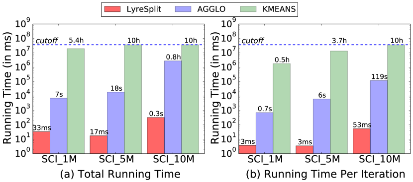
Figure 10: Algorithms’ Running Time Comparison (SCI_*)

Figure 11: Algorithms’ Running Time Comparison (CUR_*)

Efficiency Comparison.

Summary of Comparison of Running Time of Partitioning Algorithms. When minimizing the checkout time under a storage constraint (Problem 1), LyreSplit is on average $10^{3}\times$ faster than Agglo, and more than $10^{5}\times$ faster than Kmeans for all SCI_* and CUR_* datasets.

As discussed, given a storage constraint in Problem 1, we use binary search to find the best $\delta$, $BC$, and $K$ for LyreSplit, Agglo and Kmeans respectively. In this experiment, we set the storage threshold as $\gamma=2|R|$, and terminate the binary search process when the resulting storage cost $\mathcal{S}$ meets the constraint: $0.99\gamma\leq\mathcal{S}\leq\gamma$. Figure 10a and 11a shows the total running time during the end-to-end binary search process, while Figure 10b and 11b shows the running time per binary search iteration. Again, we terminate Kmeans and Agglo when the running time exceeds 10 hours, thus we cap the running time in Figure 10 and 11 at 10 hours. We can see that LyreSplit takes much less time than Agglo and Kmeans. Consider the largest dataset SCI_10M in Figure 10 as an example: with LyreSplit the entire binary search procedure and each binary search iteration took 0.3s and 53ms respectively; Agglo takes 50 minutes in total; while Kmeans does not even finish a single iteration in 10 hours.

Overall, LyreSplit is $10^{2}\times$ faster than Agglo for SCI_1M, $10^{3}\times$ faster for SCI_5M, and $10^{4}\times$ faster for SCI_10M respectively (and is $10^{3}\times$ faster than Agglo for CUR_1M and CUR_5M and $10^{5}\times$ faster for CUR_10M respectively), and more than $10^{5}\times$ faster than Kmeans for all datasets. This is mainly because LyreSplit only needs to operate on the version graph while Agglo and Kmeans operate on the version-record bipartite graph, which is much larger than the version graph. Furthermore, Kmeans can only finish the binary search process within 10 hours for SCI_1M and CUR_1M. This algorithm is extremely slow due to the pairwise comparison between each version with each centroid in each iteration, especially when the number of centroids $K$ is large. Referring back to Figure 9(f), the running times for the left-most point on the Kmeans line takes 3.6h with $K=5$, while the right-most point takes 8.8h with $K=10$. Thus our proposed LyreSplit is much more scalable than Agglo and Kmeans. Even though Kmeans is closer to LyreSplit in performance (as seen in the previous experiments), it is impossible to use in practice.

5.3 Benefits of Partitioning

Summary of Checkout Time Comparison with and without Partitioning: With only a $2\times$ increase on the storage, we can achieve a substantial $3\times$, $10\times$ and $21\times$ reduction on checkout time for SCI_1M, SCI_5M, and SCI_10M, and $3\times$, $7\times$ and $9\times$ reduction for CUR_1M, CUR_5M, and CUR_10M respectively.

We now study the impact of partitioning and demonstrate that with a relatively small increase in storage, the checkout time can be substantially reduced. We conduct two sets of experiments with the storage threshold as $\gamma=1.5\times|R|$ and $\gamma=2\times|R|$ respectively, and compare the average checkout time with and without partitioning. Figure 12 and 13 illustrate the comparison on checkout time and storage size for SCI_* and CUR_* respectively. Each collection of bars in Figure 12 and Figure 13 corresponds to one dataset. Consider SCI_5M in Figure 12 as an example: the checkout time without partitioning is 16.6s while the storage size is 2.04GB; when the storage threshold is set to be $\gamma=2\times|R|$, the checkout time after partitioning is 1.71s and the storage size is 3.97GB. As illustrated in Figure 12, with only $2\times$ increase in the storage size, we can achieve $3\times$ reduction on SCI_1M, $10\times$ reduction on SCI_5M, and $21\times$ reduction on SCI_10M for the average checkout time compared to that without partitioning. Thus, with partitioning, we can eliminate the time for accessing irrelevant records. Consequently, the checkout time remains small even for large datasets.

The results shown in Figure 13 are similar to those in Figure 12: with $2\times$ increase on the storage size, we can achieve $3\times$ reduction on CUR_1M, $7\times$ reduction on CUR_5M, and $9\times$ reduction on CUR_10M for average checkout time compared to that without partitioning. However, the reduction in Figure 13a is smaller than that in Figure 12a. The reason is the following. We can see that the checkout time without partitioning is similar for SCI and CUR datasets, but the checkout time after partitioning for CUR dataset is greater than the corresponding SCI dataset. This is because the average number of records in each version, i.e., $\frac{|E|}{|V|}$, in CUR is around 3 to 4 times greater than that in the corresponding SCI, as depicted in Table 2. Recall that $\frac{|E|}{|V|}$ is the minimal checkout cost $\mathcal{C}_{avg}$ after partitioning as stated in Observation 1. Thus, the smallest possible checkout time for CUR, which is where the blue lines with triangle markers (corresponding to LyreSplit) in Figure 9(d)(e)(f) converges to, is typically larger than that for the corresponding SCI in Figure 9(a)(b)(c). Overall, as demonstrated in Figure 12 and 13, with a small increase in the storage size, we can reduce the average checkout time to within a few seconds even when the number of records in a cvd increases dramatically. Referring back to our motivating experiment in Figure 3(c), we claim that with partitioning the checkout time using split-by-rlist is comparable to that by a-table-per-version.

Figure 12: Comparison With and Without Partitioning

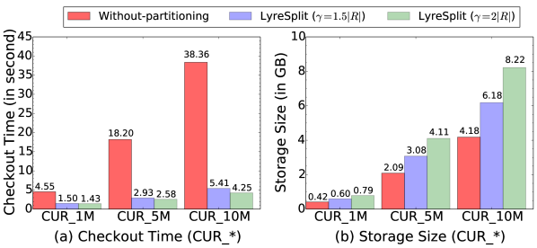
Figure 13: Comparison With and Without Partitioning

5.4 Maintenance and Migration

We now evaluate the performance of OrpheusDB’s partitioning optimizer over the course of an extended period with many versions being committed to the system. We employ our SCI_10M dataset, which contains the largest number of versions (i.e. $10k$). Here, the versions are streaming in continuously; as each version commits, we perform online maintenance based on the mechanism described in Section 4.3. When $\frac{\mathcal{C}_{avg}}{\mathcal{C}^{*}_{avg}}$ reaches the tolerance factor $\mu$, the migration engine is automatically invoked, and starts to perform the migration of data from the old partitions to the new ones identified by LyreSplit. We first examine how our online maintenance performs, and how frequently migration is invoked. Next, we test the latency of our proposed migration approach. The storage threshold is set to be $\gamma=1.5|R|$ and $\gamma=2|R|$ respectively.

Online Maintenance.

Summary of Online Maintenance Compared to LyreSplit. With our proposed online maintenance mechanism, the checkout cost $\mathcal{C}_{avg}$ diverges slowly from the best checkout cost $\mathcal{C}^{*}_{avg}$ identified by LyreSplit. When $\mu=1.5$, our migration engine is triggered only 7 and 4 times across a total of 10,000 committed versions when $\gamma=1.5|R|$ and $\gamma=2|R|$ respectively.

As shown in Figure 14(a) and 15(a), the red line depicts the best checkout cost $\mathcal{C}^{*}_{avg}$ identified by LyreSplit (note that LyreSplit is lightweight and can be run very quickly after every commit), while the blue and green lines illustrate the current checkout cost $\mathcal{C}_{avg}$ with tolerance factor $\mu=1.5$ and $\mu=2$, respectively. We can see that with online maintenance, the checkout cost $\mathcal{C}_{avg}$ (blue and green lines) starts to diverge from $\mathcal{C}^{*}_{avg}$ (red line). When $\frac{\mathcal{C}_{avg}}{\mathcal{C}^{*}_{avg}}$ exceeds the tolerance factor $\mu$, the migration engine is invoked, and the blue and green lines jump back to the red line once migration is complete. With the increase of $\mu$, the frequency of triggering migration decreases. As depicted in Figure 14(a), when $\mu=1.5$, migration is triggered 7 times, while it is only triggered 3 times when $\mu=2$, across a total of 10000 versions committed. Thus, our proposed online maintenance performs well, diverging slowly from LyreSplit. This can be explained by the same intuition shared by the online maintenance scheme and LyreSplit.

(a) Online Maintenance

(b) Migration Time

Figure 14: Online Partitioning and Migration ($\gamma=1.5|R|$)

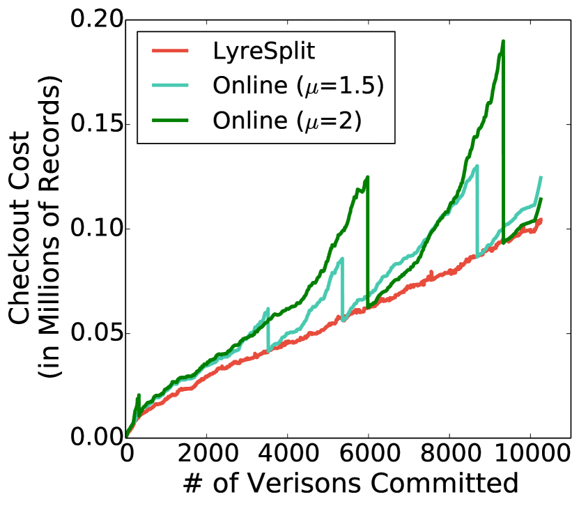
(a) Online Maintenance

(b) Migration Time

Figure 15: Online Partitioning and Migration ($\gamma=2|R|$)

Migration Time.

Summary of Comparison of Running Time of Migration. When $\mu=1.05$, the migration time with our proposed method is on average $\frac{1}{10}$ of that with naive approach of rebuilding the partitions from scratch when $\gamma=1.5|R|$ and $\gamma=2|R|$. As $\mu$ decreases, the migration time with our proposed method decreases.

Figure 14(b) and 15(b) depict the migration time when the migration engine is invoked. Figure 14(b) is in correspondence with Figure 14(a) sharing the same x-axis. For instance, with $\mu=2$, when the $5024^{th}$ version commits, the migration engine is invoked as shown by the green line in Figure 14(a). Correspondingly, the migration takes place, and we record the migration time with the green circle ($\mu=2$) in Figure 14(b). Hence, there are three green circles in Figure 14(b), corresponding to the three migrations in Figure 14(a). Same are Figure 15(a) and Figure 15(b).

We now compare our intelligent migration approach from Section 4.3, denoted intell, with the naive approach of rebuilding partitions from scratch, denoted naive. The points with upward triangles in Figure 14(b) all have $\mu=1.05$, with the red points representing intell, and the brown representing naive: we see that intell takes at most $\frac{1}{3}$, and on average $\frac{1}{10}$ of the time of naive. For the sake of clarity, we omit the migration times for different $\mu$ using naive, since they roughly fall on the same line as that of $\mu=1.05$. Next, consider the migration time with different $\mu$ using intell. Overall, as $\mu$ decreases, the migration time decreases. To see this, one can connect the points corresponding to each $\mu$ (denoted using different markers) to form lines in Figure 14(b). When $\mu$ is smaller, migration takes place more frequently, due to which the new partitioning scheme identified by LyreSplit is more similar to the current one, and hence fewer modifications need to be performed. Essentially, we are amortizing the migration cost across multiple migrations. Similar results can be found in Figure 15 when $\gamma=2|R|$.

6 Related Work

We now survey work from multiple areas related to OrpheusDB.

Dataset Version Control. A recent vision paper on Datahub [12] acknowledges the need for database systems to support collaborative data analytics—we execute on that vision by supporting collaborative analytics using a traditional relational database, thereby seamlessly leveraging the sophisticated analysis capabilities. Decibel [37] describes a new version-oriented storage engine designed “from the ground up” to support versioning. Unfortunately, the architecture involves several choices that make it impossible to support within a traditional relational database without substantial changes at all layers of the stack. For example, the eventual solution requires the system to log and query tuple membership on compressed bitmaps, reason about and operate on “delta files”, and execute new and fairly complex algorithms for even simple operations such as branch (in our case checkout) or merge (in our case commit). It remains to be seen how this storage engine can be made to interact with other components, such as the parser, the transaction manager, and the query optimizer, and all the other benefits that come “for free” with a relational database. We are approaching the problem from a different angle—the angle of reuse: how do we leverage relational databases to support versioning without any substantial changes to existing databases, which have massive adoption and open-source development that we can tap into. Recent work on the principles of dataset versioning is also relevant [13] in that it shares the concerns of minimizing storage and recreation cost; however, the paper considered the unstructured setting from an algorithmic viewpoint, and did not aim to build a full-fledged dataset versioning system. Lastly, Chavan et al. [15] describe a query language for versioning and provenance, but do not develop a system that can support such a language—our system can support an important subset of this language already.

The problem of incremental view maintenance, e.g., [9], is also related since it implicitly considers the question of storage versus query efficiency, which is one of the primary concerns in data versioning. However, the considerations and challenges are very different, making the solutions not applicable to data versioning. Finally, Buneman et al. [14] introduce a range encoding approach to track the versioning of hierarchical data in scientific databases, but their method focuses on XML data and is not applicable to the relational datasets.

Temporal Databases. There is a rich body of work on time travel (or temporal) databases, e.g., [10, 46, 47, 25, 41, 49], focusing on data management when the state of the data at a specific time is important. Temporal databases support a linear clock, or a linear chain of versions, whereas our work focuses on enabling non-linear histories. There has been some work on developing temporal databases by “bolting-on” capabilities to a traditional database [50], with DB2 [16, 45] and Teradata [11] supporting time-travel in this way. Other systems adopt an “in-database” approach [29]. For example, the SAP HANA database [20] maintains a Timeline Index [29] to efficiently support temporal join, aggregation, and time travel. Kaufmann et al. [30] provide a good summary of the temporal features in databases, while Kulkarni et al. [31] describe the temporal features in SQL2011.

The canonical approach to recording time in temporal databases is via attributes indicating the start and end time, which differs a bit depending on whether the time is the “transaction time” or the “valid time”. In either case, if one extends temporal databases to support arrays capturing versions instead of the start and end time, we will end up as a solution like the one in Figure 1b, which as shown severely limits performance. Thus, the techniques we describe in the paper on evaluating efficient data models and partitioning are still relevant and complement this prior work.

Most work in this area focuses on supporting constructs that do not directly apply to OrpheusDB, due to the lack of time-oriented notions such as: (a) queries that probe interval related-properties, such as which tuples were valid in a specific time interval, via range indexes [43], or queries that roll back to specific points [35]; (b) temporal aggregation [29] to aggregate some attributes for every time interval granularity, and temporal join [23] to join tuples if they overlap in time; (c) queries that involve time-related constructs such as AS OF, OVERLAPS, PRECEDES.

There has been limited work on branched temporal databases [33, 44], with multiple chains of linear evolution as opposed to arbitrary branching and merging. While there has been some work on developing indexing [34, 26] techniques in that context, these techniques are specifically tailored for queries that select a specific branch, and a time-window within that branch, which therefore have no correspondences in our context. Moreover, these techniques require substantial modifications to the underlying database.

Restricted Dataset Versioning. There have been some open-source projects on versioning topics related to OrpheusDB. For example, LiquiBase [6] tracks schema evolution as the only applicable modifications giving rise to new versions: in our case, we focus primarily on the data-level modifications, but also support schema modifications. On the other hand, DBV [4] is focused on recording SQL operations that give rise to new versions such that these operations can be “replayed” on new datasets—thus the emphasis is on reuse of workflows rather than on efficient versioning. As other recent projects, Dat [2] can be used to share and sync local copies of dataset across machines, while Mode [7] integrates various analytics tools into a collaborative data analysis platform. However, neither of the tools are focused on providing advanced querying and versioning capabilities. In addition, git and svn can be made to support dataset versioning, however, recent work shows these techniques are not efficient [37], and do not support sophisticated querying.

Graph Partitioning. There has been a lot of work on graph partitioning [27, 36, 21, 28], with applications ranging from distributed systems and parallel computing, to search engine indexing. The state-of-the-art in this space is NScale [42], which proposes algorithms to pack subgraphs into the minimum number of partitions while keeping the computation load balanced across partitions. In our setting, the versions are related to each other in very specific ways; and by exploiting these properties, our algorithms are able to beat the NScale ones in terms of performance, while also providing a $10^{3}$$\times$ speedup. Kumar et al. [32] study workload-aware graph partitioning by performing balanced k-way cuts on the tuple-query hypergraph for data placement and replication on the cloud; in their context, however, queries are allowed to touch multiple partitions.

7 Conclusions

We presented OrpheusDB, a dataset version control system that is “bolted on” a relational database, thereby seamlessly benefiting from advanced querying as well as versioning capabilities. We proposed and evaluated four data models for storing cvds in a database. We further optimized the best data model (split-by-rlist) via the LyreSplit algorithm that applies intelligent but lightweight partitioning to reduce the amount of irrelevant data that is read during checkout. We also adapt LyreSplit to operate in an incremental fashion as new versions are introduced. Our experimental results demonstrate that LyreSplit is 10${}^{3}\times$ faster in finding the effective partitioning scheme compared to other algorithms, can improve the checkout performance up to 20$\times$ relative to schemes without partitioning, and is capable of operating efficiently (with relatively few and efficient migrations) in a dynamic setting.

Symb.	Description	Symb.	Description
$G$	bipartite graph	$E$	bipartite edge set in $G$
$V$	version set in $G$	$n$	total number of versions
$R$	record set in $G$	$m$	total number of records
$v_{i}$	version $i$ in $V$	$r_{j}$	record $j$ in $R$
$\mathcal{P}_{k}$	$k^{th}$ partition	$\mathcal{V}_{k}$	version set in $\mathcal{P}_{k}$
$\mathcal{R}_{k}$	record set in $\mathcal{P}_{k}$	$\mathcal{E}_{k}$	bipartite edge set set in $\mathcal{P}_{k}$
$\mathcal{S}$	total storage cost	$\gamma$	storage threshold
$\mathcal{C}_{i}$	checout cost for $v_{i}$	$\mathcal{C}_{avg}$	average checkout cost
$\mathbb{G}$	version graph	$\mathbb{V}$	version set in $\mathbb{G}$
$\mathbb{E}$	edge set in $\mathbb{G}$	$e$	$e=(v_{i},v_{j})$: $v_{i}$ derives $v_{j}$
$\mathbb{T}$	version tree	$e.w$	# of common records on $e$
$l(v_{i})$	level # of $v_{i}$ in $\mathbb{G}$	$p(v_{i})$	parent version(s) of $v_{i}$ in $\mathbb{G}$
$R(v_{i})$	record set in $v_{i}$	$\ell$	# of recursive levels in Alg 1

Table 3: Notations

Appendix A Proof of Theorem 1

Proof A.7.

We reduce the well known NP-hard 3-partition problem to our Problem 1. The 3-partition problem is defined as follows: Given an integer set $\mathcal{A}=\{a_{1},\cdots,a_{n}\}$ where $n$ is divisible by 3, partition $\mathcal{A}$ into $\frac{n}{3}$ sets {$A_{1},A_{2},A_{j}\cdots A_{\frac{n}{3}}$} such that for any $A_{j}$, $\sum_{a_{i}\in A_{j}}a_{i}=\frac{B}{n/3}$ where $B=\sum_{a_{i}\in\mathcal{A}}a_{i}$.

To reduce 3-partition to our Problem 1, we first construct a version-record bipartite graph $G=(V,R,E)$ (Figure 16) that consists of $B$ versions and $(B+D)$ records, where $D$ is the number of dummy records and can be any positive integer. Specifically:

• For each integer $a_{i}\in\mathcal{A}$:

  • Create $a_{i}$ versions $\{v_{i}^{1},v_{i}^{2},\cdots,v_{i}^{a_{i}}\}$ in $V$;

  • Create $a_{i}$ records $\{r_{i}^{1},r_{i}^{2},\cdots,r_{i}^{a_{i}}\}$ in $R$;

  • Connect each $v_{i}^{j}$ with $r_{i}^{\tau}$ in $E$, where $1\leq j\leq a_{i}$ and $1\leq\tau\leq a_{i}$. This forms a biclique between $\{v_{i}^{1},\cdots,v_{i}^{a_{i}}\}$ and $\{r_{i}^{1},\cdots,r_{i}^{a_{i}}\}$.

• We also create dummy records $R_{D}$ and edges $E_{D}$:

  • $R_{D}$: create $D$ dummy records $R_{D}=\{r_{0}^{1},r_{0}^{2},\cdots,r_{0}^{D}\}$ in $R$, where $D\geq 1$;

  • $E_{D}$: connect each dummy record with every version $v\in V$.

Figure 16: An Example of a Constructed Graph $G$

As inputs to Problem 1, we take the constructed graph $G$ and set storage threshold $\gamma=\frac{n}{3}\cdot D+B$. We have the following two claims for the optimal solution to Problem 1:

Claim 1. For each $a_{i}$, its corresponding versions $\{v_{i}^{1},v_{i}^{2},\cdots,v_{i}^{a_{i}}\}$ must be in the same partition.

Claim 2. The optimal solution must have $\frac{n}{3}$ partitions, i.e, $K=\frac{n}{3}$.

We prove our first claim by contradiction. For a fixed $a_{i}$, if $\{v_{i}^{1},v_{i}^{2},\cdots,v_{i}^{a_{i}}\}$ are in different partitions, denoted as $P^{\prime}=\{\mathcal{P}_{\tau_{1}},$ $\mathcal{P}_{\tau_{2}},\cdots\}$, we can reduce the average checkout cost while maintaining the same storage cost by moving all these versions into the same partition $\mathcal{P}_{k^{*}}\in P^{\prime}$ with the smallest $|\mathcal{R}_{k^{*}}|$. Furthermore, the only common records between $v_{i}^{x}$ and $v_{j}^{y}$, where $i\neq j$, are the dummy records in $R_{D}$, thus only these dummy records will be duplicated across different partitions. Consequently, the total storage cost from records except the dummy record, i.e., $R\setminus R_{D}$, in all partitions is a constant $B$, regardless of the partitioning scheme.

Based on the first claim, we have $|\mathcal{R}_{k}|=|\mathcal{V}_{k}|+D,\forall k$ and our optimization objective function can be represented as follows:

$$\small\begin{split}\mathcal{C}_{avg}&=\frac{1}{B}\sum_{k=1}^{K}|\mathcal{V}_{k}|\times(|\mathcal{V}_{k}|+D)=\frac{1}{B}(\sum_{k=1}^{K}|\mathcal{V}_{k}|^{2}+B\cdot D)\end{split}\vspace{-3pt}$$ (A.1)

Next, we prove the correctness of our second claim. First, we show that keeping the total storage cost $\sum_{k=1}^{K}|\mathcal{R}_{k}|\leq\frac{n}{3}\times D+B$ is equivalent to keeping the number of partitions $K\leq\frac{n}{3}$. From our first claim, we know that no record in $R\setminus R_{D}$ will be duplicated and the total number of records that corresponds to $R\setminus R_{D}$ in all of the partitions is $B$. On the other hand, each partition $\mathcal{P}_{k}$ must include all dummy records $R_{D}$, which is of size $D$. Thus, the number of partitions $K$ must be no larger than $\frac{n}{3}$. Furthermore, we claim that the optimal solution must have $\frac{n}{3}$ partitions, i.e., $K=\frac{n}{3}$; otherwise, we can easily reduce the checkout cost by splitting any partition into multiple partitions.

Lastly, we prove that the optimal $\mathcal{C}_{avg}$ equals $B/K+D$ if and only if the decision problem to 3-partition is correct. First, since $\sum_{k=1}^{K}|\mathcal{V}_{k}|=B$, $\mathcal{C}_{avg}$ in Equation A.1 is minimized when all $|\mathcal{V}_{k}|=B/K,\forall k$. Returning to the 3-partition problem, if our decision to 3-partition is true, then we can partition the versions in the constructed graph $G$ accordingly and $\mathcal{C}_{avg}=B/K+D$ with each $|\mathcal{V}_{k}|=\frac{B}{K}=\frac{B}{n/3}$. Second, if the decision problem is false, then $\mathcal{C}_{avg}$ must be larger than $B/K+D$. Otherwise, all $|\mathcal{V}_{k}|$ must be the same and equal to $B/K$. Subsequently, we can easily partition $\mathcal{A}$ into $\frac{n}{3}$ sets with equal sum for 3-partition, which contradicts the assumption that the decision problem is false.

Appendix B Analysis of $\delta$

Given a storage budget $\gamma$ in Problem 1, we can simply perform a binary search on $\delta$ and get the best $\delta$ as the input for Algorithm 1. This claim is evidenced by the fact that the same sequence of edges are snipped for different $\delta$. In general, as $\delta$ increases, there are more partitions, consequently less checkout cost and larger storage cost.

Superset property of $\delta$. Consider two different $\delta$: $\delta_{1}$ and $\delta_{2}$, without loss of generality we assume $\delta_{1}<\delta_{2}$, and to simplify the analysis we pick the smallest weight as the splitting edge in each iteration. First we claim that Algorithm 1 takes more iterations when $\delta=\delta_{2}$ than $\delta=\delta_{1}$. This is because $\delta_{1}<\delta_{2}$ and the termination constraint is $|R||V|<\frac{|E|}{\delta}$. Next, we assert that the edges cut when $\delta=\delta_{1}$ is a subset of the same sequence of $\delta=\delta_{2}$. This is because in each iteration, the edge with the smallest weight is cut for both $\delta_{1}$ and $\delta_{2}$, and when $\delta_{1}$ terminates ($|R||V|<\frac{|E|}{\delta_{1}}$), $\delta_{2}$ may still goes on since $|R||V|\geq\frac{|E|}{\delta_{2}}$. Thus, compared to $\delta_{1}$, $\delta_{2}$ has more splits, larger storage cost, and less checkout cost.

Binary search on $\delta$. Initially, the search space for $\delta$ is $[\frac{|E|}{|R||V|},1]$, where each version is stored in a separate partiton(i.e., $\delta=1$) and all versions are in the same partition(i.e., $\delta=\frac{|E|}{|R||V|}$). We first try $\delta=\frac{1}{2}(\frac{|E|}{|R||V|}+1)$ in Algorithm 1 and get the resulting storage cost $\mathcal{S}$ after partitioning. If $\mathcal{S}<\gamma$, then the search space for $\delta$ is reduced to $[\frac{1}{2}(\frac{|E|}{|R||V|}+1),1]$; otherwise, $[\frac{|E|}{|R||V|},\frac{1}{2}(\frac{|E|}{|R||V|}+1)]$. Repeat this process until $0.99\gamma\leq\mathcal{S}\leq\gamma$.

Appendix C Extensions

C.1 Version graph is a DAG

When there are merges between versions, the version graph $\mathbb{G}=(\mathbb{V},\mathbb{E})$ is a DAG. We can simply transform the $\mathbb{G}$ to a version tree $\hat{\mathbb{T}}$ and then apply LyreSplit as before. Specifically, for each vertex $v_{i}\in\mathbb{V}$, if there are multiple incoming edges, we retain the edge with the highest weight and remove all other incoming edges. In other words, for each merge operation in the version graph $\mathbb{G}$, e.g., where $v_{i}$ is merged with $v_{j}$ to obtain $v_{k}$, the corresponding operation in $\hat{\mathbb{T}}$ with the removed edge $(v_{j},v_{k})$ is to inherit records only from one parent $v_{i}$ and (conceptually) create new records in the cvd for all other records in $v_{k}$ even though some records have exactly the same value as that in $v_{j}$.

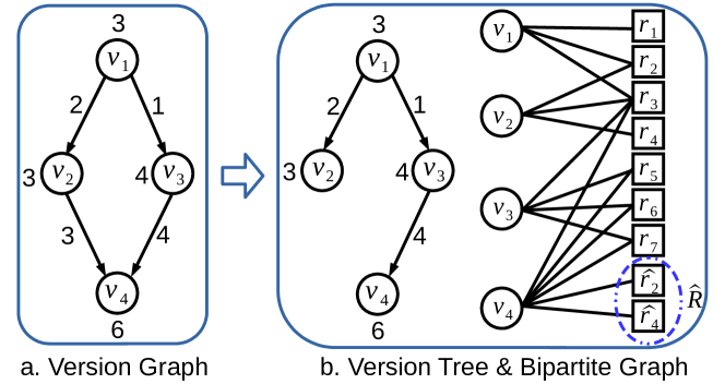
Figure 17: $\hat{\mathbb{T}}$ and $\hat{G}$ for $\mathbb{G}$ in Figure 4

For example, for the version graph $\mathbb{G}$ shown in Figure 17(a), its version $v_{4}$ has two parent versions $v_{2}$ and $v_{3}$. Since $3=w(v_{2},v_{4})<w(v_{3},v_{4})=4$, we remove edge $(v_{2},v_{4})$ from $\mathbb{G}$ and obtain the version tree $\hat{\mathbb{T}}$ in Figure 17(b). Moreover, conceptually, we can draw a bipartite graph $\hat{G}$ corresponding to $\hat{\mathbb{T}}$ as shown in Figure 17(b) with two duplicated records, i.e., $\{\hat{r_{2}},\hat{r_{4}}\}$. That is, $v_{4}$ in $\hat{\mathbb{T}}$ inherits 4 records from $v_{3}$ and creates two new records $\hat{R}=\{\hat{r_{2}},\hat{r_{4}}\}$ even though $\hat{r_{2}}$ ($\hat{r_{4}}$) is exactly the same as $r_{2}$ ($r_{4}$). Thus, we have 9 records with $|\hat{R}|=2$ and 16 bipartite edges in Figure 17(b).

Performance analysis. The number of bipartite edges in the bipartite graph $\hat{G}$ (corresponding to $\hat{\mathbb{T}}$) is the same as that in $G$ (corresponding to $\mathbb{G}$), i.e., $|E|$. However, compared to $G$, the number of records in $\hat{G}$ is larger, i.e., $|R|+|\hat{R}|$, where $R$ is the set of records in the original version-record bipartite graph $G$ and $\hat{R}$ is the set of duplicated records. According to Theorem 4.5, given $\delta$, LyreSplit provides a partitioning scheme with the checkout cost within $\frac{1}{\delta}\cdot\frac{|E|}{|V|}$ and the storage cost within $(1+\delta)^{\ell}(|R|+|\hat{R}|)$. We formally state the performance guarantee in Theorem C.8. Moreover, this analysis is obtained by treating $\hat{R}$ as different from $R$ when calculating the storage cost and checkout cost. In post-processing, we can combine $\hat{R}$ with $R$ when calculating the real storage cost and checkout cost, making the real $\mathcal{S}$ and $\mathcal{C}_{avg}$ even smaller.

Theorem C.8.

Given a version graph $\mathbb{G}$ with merges and a parameter $\delta$, LyreSplit results in a $(\frac{|R|+|\hat{R}|}{|R|}(1+\delta)^{\ell},\frac{1}{\delta})$-approximation for partitioning.

C.2 Weighted Checkout Cost

In this section, we focus on the weighted checkout cost case, where versions are checked out with different frequencies.

Problem formulation. Let $\mathcal{C}_{w}$ denote the weighted checkout cost; say version $v_{i}$ is checked out with probability or frequency $f_{i}$ Then the weighted checkout cost $\mathcal{C}_{w}$ can be represented as $\mathcal{C}_{w}=\frac{\sum_{i=1}^{n}(f_{i}\times\mathcal{C}_{i})}{\sum_{i=1}^{n}f_{i}}$. With this weighted checkout cost, we can modify the problem formulation for Problem 1 by simply replacing $\mathcal{C}_{avg}$ with $\mathcal{C}_{w}$.

Proposed Algorithm. Without the loss of generality, we assume that $f_{i}$ for any version $v_{i}$ is an integer. Given a version tree $\mathbb{T}=(\mathbb{V},\mathbb{E})$ and the frequency $f_{i}$ for each version $v_{i}$, we construct a version tree $\mathbb{T}^{\prime}=(\mathbb{V}^{\prime},\mathbb{E}^{\prime})$ in the following way:

• For each version $v_{i}\in\mathbb{V}$:

  • $\mathbb{V}^{\prime}$: Create $f_{i}$ versions $\{v_{i}^{1},v_{i}^{2},\cdots,v_{i}^{f_{i}}\}$ in $\mathbb{V}^{\prime}$;

  • $\mathbb{E}^{\prime}$: Connect $v_{i}^{j}$ with $v_{i}^{j+1}$ to form a chain in $\mathbb{E}^{\prime}$, where $1\leq j<f_{i}$

• For each edge $(v_{i},v_{j})\in\mathbb{E}$:

  • $\mathbb{E}^{\prime}$: Connect $v_{i}^{f_{i}}$ with $v_{j}^{1}$ in $\mathbb{E}^{\prime}$

The basic idea of constructing $\mathbb{T}^{\prime}$ is to duplicate each version $v_{i}\in\mathbb{V}$ $f_{i}$ times. Afterwards, we apply LyreSplit directly on $\mathbb{T}^{\prime}$ to obtain the partitioning scheme. However, after partitioning, $v_{i}^{j}\in\mathbb{V}^{\prime}$ with the same $i$ may be assigned to different partitions, denoted as $P^{\prime}$. Thus, as a post process, we move all $v_{i}^{j}$ ($1\leq j\leq f_{i}$) into the same partition $\mathcal{P}\in P^{\prime}$ that has the smallest number of records. Correspondingly, we get a partitioning scheme for $\mathbb{V}$, i.e., for each $v_{i}\in\mathbb{V}$, assign it to the partition where $v_{i}^{j}\in\mathbb{V}^{\prime}$ ($1\leq j\leq f_{i}$) is in.

Performance analysis. At one extreme, when each version is stored in a separate table, the checkout cost $\mathcal{C}_{w}$ for $\mathbb{T}$ is the lowest with each $\mathcal{C}_{i}=|R(v_{i})|$, the number of records in version $v_{i}$; thus, $\mathcal{C}_{w}=\frac{\sum_{i=1}^{n}(f_{i}\times|R(v_{i})|)}{\sum_{i=1}^{n}f_{i}}$, denoted as $\zeta$. At the other extreme, when all versions are stored in a single partition, the total storage cost is the smallest, i.e., $|R|$. In the following, we study the performance of the extended algorithm in the weighted case, and compare the storage cost and weighted checkout cost with $|R|$ and $\zeta$ respectively.

First, consider the bipartite graph $G^{\prime}=(V^{\prime},R^{\prime},E^{\prime})$ corresponding to the constructed version tree $\mathbb{T}^{\prime}$. The number of versions $|V^{\prime}|$ equals $\sum_{i=1}^{n}f_{i}$, since there are $f_{i}$ replications for each version $v_{i}$; the number of records $|R^{\prime}|$ is the same as $|R|$, since there are no new records added; the number of bipartite edges $|E^{\prime}|$ is $\sum_{i=1}^{n}(\sum_{j=1}^{f_{i}}|R(v_{i}^{j})|)=\sum_{i=1}^{n}(f_{i}\times|R(v_{i})|)$, since the number of records in each version $v_{i}^{j}$ with the same $i$ is in fact $|R(v_{i})|$. Next, based on Theorem 4.5, the average checkout cost after appyling Algorithm 1 is within $\frac{1}{\delta}\cdot\frac{|E^{\prime}|}{|V^{\prime}|}=\frac{1}{\delta}\cdot\frac{\sum_{i=1}^{n}(f_{i}\times|R(v_{i})|)}{\sum_{i=1}^{n}f_{i}}=\frac{1}{\delta}\cdot\zeta$, while the storage cost is within $(1+\delta)^{\ell}\cdot|R^{\prime}|=(1+\delta)^{\ell}\cdot|R|$, where $\ell$ is the termination level in Algorithm 1. After post-processing, the total storage cost as well the average checkout cost decreases since we pick the partition with the smallest number of records for all $v_{i}^{j}$ with a fixed $i$. At last, note that after mapping the partitioning scheme from $\mathbb{T}^{\prime}$ to $\mathbb{T}$, the total storage cost and the average (unweighted) checkout cost for $\mathbb{T}^{\prime}$ are in fact the total storage cost and the weighted checkout cost for $\mathbb{T}$ respectively. Thus, with the extended algorithm, we achieve the same approximation bound as in Theorem 4.5 with respect to the lowest storage cost and weighted checkout cost, i.e., in the weighted checkout case, our algorithm also results in $((1+\delta)^{\ell},\frac{1}{\delta})$-approximation for partitioning.

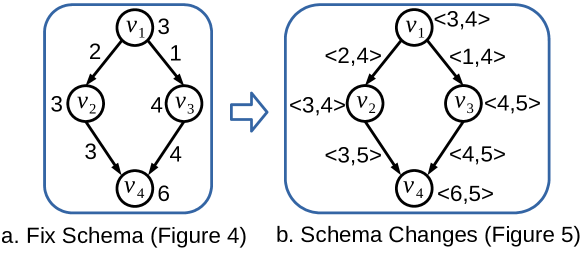
Figure 18: Version Graph $\mathbb{G}$ with/without Schema Changes

Figure 19: Checkout Cost Model Validation

C.3 Schema Changes

Our algorithm can be adapted to the single-pool setting described in Section 3.3 with schema changes. Recall the examples in Figure 4 and 5, corresponding to the fixed and dynamic schema settings. Figure 18a only maintains the number of records in each node (version), and the number of common records between two versions for each edge. In addition, Figure 18b also records the number of attributes and common attributes for each node and edge respectively. For instance, $v_{3}$ has five attributes and shares four common attributes with $v_{1}$.

Given a version graph, let $A$ be the total number of attributes in all versions. For instance, Figure 18b, corresponding to Figure 5, has five attributes in total. Without partitioning, the storage cost and the checkout cost can be represented as $\mathcal{S}=|A||R|$ and $\mathcal{C}_{avg}=|A||R|$ respectively, where $|R|$ is the number of records. Next, let $a(v_{i})$ and $a(v_{i},v_{j})$ denote the number of attributes in version $v_{i}$ and the number of common attributes between version $v_{i}$ and $v_{j}$, respectively. Recall that $w(v_{i},v_{j})$ denotes the number of common records between version $v_{i}$ and $v_{j}$, disregarding the schema. For instance, if version $v_{j}$ is obtained by deleting an attribute from $v_{i}$, then $a(v_{i},v_{j})=a(v_{i})-1$ and $w(v_{i},v_{j})=|R(v_{i})|$.

The high-level idea is similar to LyreSplit: split an edge if its "weight" is smaller than some threshold. However, the weight here not only depends on the number of common records $w(v_{i},v_{j})$, but also the number of common atrributes $a(v_{i},v_{j})$. Specifically, if $a(v_{i},v_{j})\times w(v_{i},v_{j})\leq\delta\times|A||R|$, edge $(v_{i},v_{j})$ is considered as a candidate splitting edge. Note that when there is no schema change, $a(v_{i},v_{j})=|A|$, and the constraint is reduced to $w(v_{i},v_{j})\leq\delta|R|$ (line 5 in Algorithm 1). The remaining algorithm is the same as Algorithm 1.

Appendix D Additional Experiments

D.1 Verification of Checkout Cost Model

In this section, we both analyze and experimentally evaluate the checkout cost model proposed in Section 4.1. We demonstrate that the checkout cost $\mathcal{C}_{i}$ of a version $v_{i}$ grows linearly with the number of records in the partition $\mathcal{P}_{k}$ that contains $v_{i}$, i.e., $\mathcal{C}_{i}\propto|\mathcal{R}_{k}|$.

As depicted in the SQL query in Table 1, the checkout cost is impacted by the cost of two operations: (a) obtaining the list of records rlist associated with $v_{i}$; (b) joining data table with rlist to get all valid records. The cost from part (a) is a constant regardless of the partitioning scheme we use, and it is small since rlist can be obtained efficiently using a physical primary key index on vid. Thus, we focus our analysis on the cost from part (b).

We focus on three important types of join operations: hash-join, merge-join and nested-loop-join. In the following, we evaluate the checkout cost model for all these join algorithms and provide a detailed analysis. We vary the number of records in the checkout version ($|rlist|$) and the number of records in its corresponding partition ($|\mathcal{R}_{k}|$) in our experiments. The parameter $|\mathcal{R}_{k}|$ is varied from 1K to 30M and $|rlist|$ is varied from 1K to 1M, where rlist is a sorted list of randomly sampled rids from $\mathcal{R}_{k}$. In addition, we have two different physical layouts for the data table, one clustered on rid and another clustered on its original relation primary key (PK)— <protein1, protein2> in Figure 1. For each of the three join types, we compare the checkout time (in seconds) vs. the estimated checkout cost (in millions of records). Note that we build an index on rid in the data table, otherwise, the nested-loop-join would be very time-consuming since each outer loop requires a full scan on the inner table. The results are presented in Figure 19, where each line is plotted with a fixed $|rlist|$ (1K, 10K, 100K, and 1M respectively) and varying $|\mathcal{R}_{k}|$. We now describe the performance of the individual join algorithms below.

Hash-join. No matter which physical layout is used, the query plan for a hash-join based approach is to first build a hash table for rlist and then sequentially scan the data table with each record probing the hash table. By benefiting from the optimized implementation of the hash-join in PostgreSQL, the cost of probing each rid in the hash table is almost a constant. With fixed $|rlist|$, the building phase in hash-join is the same, while the running time in the probing phase is proportional to $|\mathcal{R}_{k}|$. Hence, as depicted in Figure 19(a) and (d), with a fixed $|rlist|$, the running time increases linearly with the growth of $|\mathcal{R}_{k}|$.

Merge-join. When the data table is clustered on rid, the query plan for a merge-join based approach is to first sort rlist obtained from the versioning table, then conduct an index scan using rid index on the data table and merge with the rlist from the versioning table. First, since rlist from the versioning table has already been sorted, quicksort can immediately terminate after the first iteration. Second, since the data table is physically clustered on rid, an index scan on rid is equivalent to a sequential scan in the data table. Thus, with fixed $|rlist|$, the running time grows linearly with the increase of $|\mathcal{R}_{k}|$, which is experimentally verified in Figure 19(b).

On the other hand, when the data table is clustered on the relation primary key, PostgreSQL gives different query plans for different $|\mathcal{R}_{k}|$. When $|\mathcal{R}_{k}|$ is equal to 4M, 6M and 8M, the query plan is the same as the above—sort rlist, conduct an index scan on rid and merge with rlist. However, since the physical layout is no longer clustered on rid, having an index scan on rid is equivalent to performing random access $|\mathcal{R}_{k}|$ times into the data table, which is very time-consuming as illustrated in Figure 19(e). For other $|\mathcal{R}_{k}|$ except 4M, 6M and 8M, the query plan is to first sort rlist from the versioning table, conduct a sequantial scan on the data table, sort the rids, and then finally merge rids with rlist. Thus, with fixed $|rlist|$, the running time is proportional to $|\mathcal{R}_{k}|$, but greater than the hash-join based approach due to the overhead of sorting, as shown by the last five points in Figure 19(e).

Index-nested-loop-join. No matter which physical layout is used, the query plan for an index-nested-loop-join based approach is to perform a random I/O in the data table for each rid in rlist from the versioning table. Consider the scenario where $|rlist|$ is fixed and the data table is clustered on rid. When $|rlist|$ is much smaller than $|\mathcal{R}_{k}|$, the running time is almost the same since each random I/O is a constant and $|rlist|$ is fixed. This is also verified by the right portion of the blue line ($|rlist|$=1K) and red line ($|rlist|$=10K) in Figure 19(c). However, when $|rlist|$ is comparable to $|\mathcal{R}_{k}|$, the running time is proportional to $|\mathcal{R}_{k}|$ as illustrated in the green ($|rlist|$=1M) and yellow ($|rlist|$=100K) line in Figure 19(c). This is because hundreds of thousands of random I/Os are eventually reduced to a full sequential scan on the data table when $\mathcal{R}_{k}$ is clustered on rid. Returning to the checkout cost model, since partitioning algorithms tend to group similar versions together, after partitioning, $|rlist|$ is very likely to be comparable to $|\mathcal{R}_{k}|$ and thus the checkout time can be quantified by $|\mathcal{R}_{k}|$. Furthermore, the yellow line ($|rlist|$=100K) in Figure 19(c) indicates that even when $\frac{|rlist|}{|\mathcal{R}_{k}|}=\frac{1}{300}$, random I/Os will still be reduced to a sequential scan, consequently the running time grows linearly with $|\mathcal{R}_{k}|$.

However, note that when the data table is not clustered on $rid$, each random I/O takes almost constant time as shown in Figure 19(f). Since random I/O is more time-consuming than sequential I/O, the index-nested-loop-join performs much worse than hash-join as shown in Figure 19(d) and (f).

Overall Takeaways. When the data table is clustered on rid, the checkout cost can be quantified by $|\mathcal{R}_{k}|$ for hash-join and merge-join based approaches; while for index-nested-loop-join, the checkout cost can also be quantified by $|\mathcal{R}_{k}|$ when $\frac{|rlist|}{|\mathcal{R}_{k}|}\geq\frac{1}{300}$, which is typically the case in the partitions after partitioning especially for latest versions. On the other hand, when the data table is not clustered on rid, the checkout cost for the hash-join based approach can still be quantified by $|\mathcal{R}_{k}|$, while the merge-join and the index-nested-loop-join based approaches perform worse than that of hash-join for most cases. Overall, a hash-join based approach has the following advantages: (a) the checkout time using hash-join does not rely on any index on rid; (b) hash-join based approach has good and stable performance regardless of the physical layout; (c) the checkout cost using hash-join is easy to model, laying foundation for further optimization on checkout time. Thus, throughout our paper we focus on hash-join for the checkout command and model the checkout cost $\mathcal{C}_{i}$ as linear in the number of records $|\mathcal{R}_{k}|$ in the partition that contains $v_{i}$.

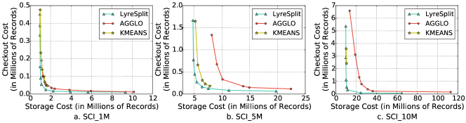
Figure 20: Estimated total Storage Cost vs. Estimated Checkout Cost (SCI_*)

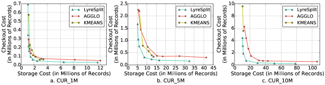
Figure 21: Estimated Storage Cost vs. Estimated Checkout Cost (CUR_*)

Figure 22: Estimated Checkout Cost vs. Real Checkout Time (SCI_*)

Figure 23: Estimated Checkout Cost vs. Real Checkout Time (CUR_*)

D.2 Estimated Storage Cost and Checkout Cost

In the main body of the paper, we performed an experimental evaluation of the trade-off between the actual checkout time and the storage size in Figure 9. One question we may have is whether our cost model has a similar trade-off. In Figure 21, we report the estimated checkout cost versus the estimated storage cost according to our model. We can see that the trend in Figure 21 is very similar to that in Figure 9. However, the absolute reduction on checkout cost in Figure 21 is typically greater than that in Figure 9. This is because we do not count the constant overhead in the estimated checkout cost. We again check the correctness of our checkout cost model by comparing the estimated checkout cost with the actual checkout time. We present the result in Figure 22 and 23. We can see that the points in Figure 22 and 23(a)(b)(c) roughly form a straight line, validating that the checkout time is linearly correlated to our cost model. Hence, we conclude that our cost modeling and problem formulation are accurate.

References

- [1] Array in MySql. https://dev.mysql.com/worklog/task/?id=2081.
- [2] Dat. http://datproject.org/.
- [3] DB2 9.7 array. https://www.ibm.com/support/knowledgecenter/SSEPGG_9.7.0/com.ibm.db2.luw.sql.ref.doc/doc/r0050497.html.
- [4] dbv. https://dbv.vizuina.com/.
- [5] For big-data scientists, ‘janitor work’ is key hurdle to insights. http://www.nytimes.com/2014/08/18/technology/for-big-data-scientists-hurdle-to-insights-is-janitor-work.html?_r=0.
- [6] Liquibase. http://www.liquibase.org/.
- [7] Mode. https://about.modeanalytics.com/.
- [8] PostgreSQL 9.5 intarray. https://www.postgresql.org/docs/current/static/intarray.html.
- [9] Y. Ahmad et al. Dbtoaster: Higher-order delta processing for dynamic, frequently fresh views. VLDB Endowment, 5(10):968–979, 2012.
- [10] I. Ahn et al. Performance evaluation of a temporal database management system. In ACM SIGMOD Record, volume 15, pages 96–107. ACM, 1986.
- [11] M. Al-Kateb et al. Temporal query processing in teradata. In EDBT’13, pages 573–578. ACM.
- [12] A. Bhardwaj, S. Bhattacherjee, A. Chavan, A. Deshpande, A. J. Elmore, S. Madden, and A. G. Parameswaran. Datahub: Collaborative data science & dataset version management at scale. CIDR, 2015.
- [13] S. Bhattacherjee, A. Chavan, S. Huang, A. Deshpande, and A. Parameswaran. Principles of dataset versioning: Exploring the recreation/storage tradeoff. VLDB, 2015.
- [14] P. Buneman, S. Khanna, K. Tajima, and W.-C. Tan. Archiving scientific data. ACM Transactions on Database Systems (TODS), 29(1):2–42, 2004.
- [15] A. Chavan, S. Huang, A. Deshpande, A. Elmore, S. Madden, and A. Parameswaran. Towards a unified query language for provenance and versioning. In TaPP 15, 2015.
- [16] C. X. Chen, J. Kong, and C. Zaniolo. Design and implementation of a temporal extension of sql. In Data Engineering, pages 689–691, 2003.
- [17] G. O. Consortium et al. Gene ontology consortium: going forward. Nucleic acids research, 43(D1):D1049–D1056, 2015.
- [18] C. De Castro, F. Grandi, and M. R. Scalas. On schema versioning in temporal databases. In Recent advances in temporal databases, pages 272–291. 1995.
- [19] C. De Castro, F. Grandi, and M. R. Scalas. Schema versioning for multitemporal relational databases. Information Systems, 22(5):249–290, 1997.
- [20] F. Färber, N. May, W. Lehner, P. Große, I. Müller, H. Rauhe, and J. Dees. The sap hana database–an architecture overview. IEEE Data Eng. Bull., 35(1):28–33, 2012.
- [21] U. Feige, D. Peleg, and G. Kortsarz. The dense k-subgraph problem. Algorithmica, 29(3):410–421, 2001.
- [22] K. Fisher, D. Walker, K. Q. Zhu, and P. White. From dirt to shovels: fully automatic tool generation from ad hoc data. In ACM SIGPLAN Notices, volume 43, pages 421–434. ACM, 2008.
- [23] D. Gao, S. Jensen, T. Snodgrass, and D. Soo. Join operations in temporal databases. The VLDB Journal, 14(1):2–29, 2005.
- [24] S. Jain, D. Moritz, D. Halperin, B. Howe, and E. Lazowska. Sqlshare: Results from a multi-year sql-as-a-service experiment. In Proceedings of the 2016 International Conference on Management of Data, pages 281–293. ACM, 2016.
- [25] C. S. Jensen and R. T. Snodgrass. Temporal data management. IEEE Transactions on Knowledge and Data Engineering, 11(1):36–44, 1999.
- [26] L. Jiang, B. Salzberg, D. B. Lomet, and M. B. García. The bt-tree: A branched and temporal access method. In VLDB, pages 451–460, 2000.
- [27] G. Karypis and V. Kumar. A fast and high quality multilevel scheme for partitioning irregular graphs. SISC, 20(1):359–392, 1998.
- [28] G. Karypis and V. Kumar. Multilevel k-way hypergraph partitioning. VLSI design, 11(3):285–300, 2000.
- [29] M. Kaufmann et al. Timeline index: A unified data structure for processing queries on temporal data in sap hana. In SIGMOD 2013, pages 1173–1184.
- [30] M. Kaufmann et al. Benchmarking bitemporal database systems: Ready for the future or stuck in the past? In EDBT, pages 738–749, 2014.
- [31] K. Kulkarni and J.-E. Michels. Temporal features in sql: 2011. ACM Sigmod Record, 41(3):34–43, 2012.
- [32] K. A. Kumar, A. Quamar, A. Deshpande, and S. Khuller. Sword: workload-aware data placement and replica selection for cloud data management systems. The VLDB Journal, 23(6):845–870, 2014.
- [33] G. M. Landau et al. Historical queries along multiple lines of time evolution. The VLDB Journal, 4(4):703–726, 1995.
- [34] S. Lanka and E. Mays. Fully persistent B+-trees, volume 20. ACM, 1991.
- [35] J. W. Lee, J. Loaiza, M. J. Stewart, W.-M. Hu, and W. H. Bridge Jr. Flashback database, Feb. 20 2007. US Patent 7,181,476.
- [36] D.-R. Liu and S. Shekhar. Partitioning similarity graphs: A framework for declustering problems. Information Systems, 21(6):475–496, 1996.
- [37] M. Maddox, D. Goehring, A. J. Elmore, S. Madden, A. Parameswaran, and A. Deshpande. Decibel: The relational dataset branching system. VLDB, 9(9):624–635, 2016.
- [38] R. J. Miller et al. The clio project: managing heterogeneity. SIGMOD Record, 30(1):78–83, 2001.
- [39] H. J. Moon et al. Scalable architecture and query optimization fortransaction-time dbs with evolving schemas. In SIGMOD 2010.
- [40] H. J. Moon et al. Managing and querying transaction-time databases under schema evolution. VLDB, 2008.
- [41] G. Ozsoyoglu and R. T. Snodgrass. Temporal and real-time databases: A survey. IEEE Transactions on Knowledge and Data Engineering, 7(4):513–532, 1995.
- [42] A. Quamar, A. Deshpande, and J. Lin. Nscale: neighborhood-centric large-scale graph analytics in the cloud. The VLDB Journal, pages 1–26, 2014.
- [43] B. Salzberg and V. J. Tsotras. Comparison of access methods for time-evolving data. ACM Computing Surveys (CSUR), 31(2):158–221, 1999.
- [44] B. J. Salzberg and D. B. Lomet. Branched and Temporal Index Structures. College of Computer Science, Northeastern University, 1995.
- [45] C. M. Saracco, M. Nicola, and L. Gandhi. A matter of time: Temporal data management in db2 for z. IBM Corporation, New York, 2010.
- [46] R. Snodgrass and I. Ahn. A taxonomy of time databases. ACM Sigmod Record, 14(4):236–246, 1985.
- [47] R. T. Snodgrass et al. Tsql2 language specification. Sigmod Record, 23(1):65–86, 1994.
- [48] D. Szklarczyk et al. The string database in 2011: functional interaction networks of proteins, globally integrated and scored. Nucleic acids research, 39(suppl 1):D561–D568, 2011.
- [49] A. U. Tansel et al. Temporal databases: theory, design, and implementation. Benjamin-Cummings Publishing Co., Inc., 1993.
- [50] K. Torp, C. S. Jensen, and R. T. Snodgrass. Stratum approaches to temporal dbms implementation. In IDEAS’98, pages 4–13. IEEE, 1998.
- [51] L. Xu, S. Huang, S. Hui, A. Elmore, and A. Parameswaran. OrpheusDB: A lightweight approach to relational dataset versioning. In SIGMOD’17 Demo (accepted), data-people.cs.illinois.edu/papers/orpheus-demo.pdf.