Variational principle for the determination of unstable periodic orbits and instanton trajectories at saddle points

Abstract

The complexity of arbitray dynamical systems and chemical reactions, in particular, can often be resolved if only the appropriate periodic orbit—in the form of a limit cycle, dividing surface, instanton trajectories or some other related structure—can be uncovered. Determining such a periodic orbit, no matter how beguilingly simple it appears, is often very challenging. We present a method for the direct construction of unstable periodic orbits and instanton trajectories at saddle points by means of Lagrangian descriptors. Such structures result from the minimization of a scalar-valued phase space function without need for any additional constraints or knowledge. We illustrate the approach for two-degree of freedom systems at a rank-1 saddle point of the underlying potential energy surface by constructing both periodic orbits at energies above the saddle point as well as instanton trajectories below the saddle point energy.

I Introduction

Periodic orbits (POs) are useful in resolving the overall dynamics in the disparate fields of chaotic dynamics,Stöckmann (1999); Grobgeld et al. (1992); Marcinek and Pollak (1994); Ott (2002); Schuster and Just (2005); Gekle et al. (2006) semiclassics,Gutzwiller (1970, 1971, 1990); Brack and Bhaduri (2003) classical reaction dynamics,Pollak (1985); Pechukas and Pollak (1977); Pollak and Pechukas (1978); Pollak and Child (1980) and tunneling processes. Miller (1975a); Coleman (1977); Callan and Coleman (1977); Affleck (1981); Stoof (1997); Wunner et al. (2008); Rommel et al. (2011); Einarsdóttir et al. (2012); Meisner and Kästner (2016) A general distinction can be made between stable and unstable POs. Integrable systems give rise to POs whose oscillations on the invariant tori can be characterized by corresponding particular frequencies. More generally, POs form limit cycles, are essential to Gutzwiller’s trace formulaGutzwiller (1970, 1971) and are crucial in semiclassical quantization theories.Miller (1974a, 1977); Hernandez and Miller (1993); Hernandez (1994) Unstable POs are of importance in the field of classical reaction dynamics in classical systems where they form recrossing-free dividing surfaces.Pollak and Pechukas (1979); Pollak (1985); Grobgeld et al. (1992); Marcinek and Pollak (1994); Bartsch et al. (2005); Hernandez et al. (2010) They are important for understanding tunneling dynamics through a barrier in quantum mechanical reactions wherein the PO on the inverted potential, $-V$, is the instanton trajectory providing the leading contribution to the path integral.Kleinert (2009) In common between all of these cases, is the invariance of POs as they provide a scaffold from which to obtain other geometric structures, and thus remain objects of current interest such as in, e.g., Refs. Janković and Dmitrašinović, 2016; Ding et al., 2016.

In many cases, the PO of interest is a rather simple trajectory, but a substantial effort is often needed to find it, if can be found at all. The requirement of periodicity, $\boldsymbol{x}(t)=\boldsymbol{x}(t+T)$ with the characteristic period $T$, is usually employed as an appropriate constraint. Specifically, root-search algorithms are employed to solve $\boldsymbol{x}(T)-\boldsymbol{x}(0)=0$ with respect to the boundary conditions: the unknown initial position $\boldsymbol{x}(0)$ on the PO, and the unknown period $T$. If the desired PO is a hyperbolic trajectory, then numerical instabilities can derail the convergence in the root-search procedure. In some such cases, it may even be impossible to integrate the PO over the whole period within the numerical accuracy of standard integrators. Multi-step integrators such as the advanced multi-shooting algorithmMorrison et al. (1962); Kiehl (1994) can help to address some of these but not all.

In this paper, we present an alternate approach for determining unstable POs at saddle points with energies above and below the corresponding saddle point energy $E^{\ddagger}$. We have found that such POs can be obtained through a variational procedure based on Lagrangian descriptors (LDs).Mendoza and Mancho (2010); Mancho et al. (2013); Craven et al. (2014a, b, 2015); Craven and Hernandez (2015); Junginger and Hernandez (2016a); Junginger et al. (2016); Junginger and Hernandez (2016b) The connection of the LD to the construction of POs is presented in Sec. II. An advantage of this procedure in avoiding the root-search algorithm is that it requires no knowledge of the boundary conditions. It is only based on minimizing the scalar-valued LD in phase space. We demonstrate the LD-PO procedure in Sec. III through the determination of unstable POs in two very different dynamical cases involving rank-1 saddle points. The first example addresses classical POs at energies above the saddle point energy, $E>E^{\ddagger}$, that are related to the dividing surface. The second example constructs instanton trajectories below the saddle point energy, $E<E^{\ddagger}$, that are related to quantum-mechanical tunneling.

II Construction of periodic orbits through Lagrangian descriptors

The LD is a scalar-valued function in phase space and for each point $(\boldsymbol{x}_{0},\boldsymbol{v}_{0})$ and time $t_{0}$. It is defined by

$$\mathcal{L}(\boldsymbol{x}_{0},\boldsymbol{v}_{0},t_{0})=\int_{t_{0}-\tau}^{t_{0}+\tau}\|\boldsymbol{v}(t)\|\,\mathrm{d}t\,.$$ (1)

Here, the integration time $\tau$ is a free parameter that has to be chosen large enough such that underlying structures of the dynamics are sufficiently resolved, and that all relevant time scales are covered. For a given $\tau$, the resulting LD is a measure of the arc length of the respective trajectory $\boldsymbol{q}(t)$ starting at $(\boldsymbol{x}_{0},\boldsymbol{v}_{0},t_{0})$ in forward and backwards time. In recent work,Craven and Hernandez (2015); Junginger and Hernandez (2016a); Craven and Hernandez (2016) our group has demonstrated that the moving dividing surface associated with the transition state trajectory is nonrecrossing. In arbitrary dimensions at each instance in time, this structure is a normally hyperbolic invariant manifold (NHIM)Fenichel (1972); Uzer et al. (2002) which can be obtained by perturbation theory.Hernandez and Miller (1993); Hernandez (1994); Jaffé et al. (2005); Komatsuzaki and Berry (1999); Waalkens and Wiggins (2004); Hernandez et al. (2010) Using extremal values of the LD, we were also able to construct the DS, itself.Craven and Hernandez (2015); Junginger and Hernandez (2016a); Craven and Hernandez (2016) Meanwhile, at constant energy on two-dimensional stationary potentials, Pollak and PechukasPollak and Pechukas (1978); Pechukas and Pollak (1979); Pollak et al. (1980) showed that the nonrecrossing dividing surface is a PO associated with the nearby saddle point. Thus the LD-PO conjecture arises from the logic of these connected arguments in two-dimensions: the trajectory which minimizes the LD is a periodic orbit associated with a saddle point.

More generally, the essential connection between the LD and PO associated with a saddle point lies in the fact that each orbit $\mathcal{P}_{E}$ at energy $E$ is located at the intersection of the stable and unstable manifolds $\mathcal{W}_{\text{s,u}}$ attached to the saddle,

$$\mathcal{P}_{E}=\mathcal{W}_{\text{s}}\cap\mathcal{W}_{\text{u}}\bigl{.}\bigr{|}_{E}\,.$$ (2)

This relation holds because any deviation of the trajectory from the PO with a nonzero unstable contribution would let the particle escape. Moreover, trajectories on both of these manifolds ($\mathcal{W}_{\text{s}}$ and $\mathcal{W}_{\text{u}}$) lead to extremal values of the LD in Eq. (1). More precisely, the manifolds correspond either to a minimum of the LD’s forward ($f$: $t_{0}\leq t\leq t_{0}+\tau$) or its backward ($b$: $t_{0}-\tau\leq t\leq t_{0}$) contribution,

$$\mathcal{W}_{\text{s}}(t_{0}) =\operatorname{arg\,min}\mathcal{L}^{\text{(f)}}(\boldsymbol{x}_{0},\boldsymbol{v}_{0},t_{0})\,,$$ (3a)

$$\mathcal{W}_{\text{u}}(t_{0}) =\operatorname{arg\,min}\mathcal{L}^{\text{(b)}}(\boldsymbol{x}_{0},\boldsymbol{v}_{0},t_{0})\,,$$ (3b)

where ‘$\operatorname{arg\,min}$’ denotes the argument of the minimum of the LD hypersurface with respect to the phase space coordinates ($\boldsymbol{x}_{0},\boldsymbol{v}_{0}$). Thus the position of the PO in phase space is directly related to the minimum of the LD (1), leading to the periodic orbit:

$$\mathcal{P}_{E}(t_{0})=\operatorname{arg\,min}\mathcal{L}(\boldsymbol{x}_{0},\boldsymbol{v}_{0},t_{0})\bigl{.}\bigr{|}_{E}\,.$$ (4)

In order to obtain the LD-PO, it is not necessary that the integration time $\tau$ of the LD coincides with the period $T$. In a numerical scheme, it is therefore possible to start a PO search optimization with short integration times providing an approximation to the PO. A subsequent increase of the integration times then improves the results and the numerical accuracy of the PO as needed.

III Applications to rank-1 saddles in two-degree of freedom systems

We illustrate the LD-PO method through two cases: the construction of the periodic orbit dividing surface (PODS),Pollak (1985); Pechukas and Pollak (1977); Pollak and Pechukas (1978); Pollak and Child (1980) and the instanton trajectory.Stoof (1997); Wunner et al. (2008) All the following results have been obtained by numerically integrating the dynamical equations corresponding to the respective given potentials using a velocity verlet algorithm. For the resulting trajectory, the LD (1) has been evaluated on the fly during the integration, and the minimization of the LD hypersurface in Eq. (4) has been performed using a standard simplex procedure.

III.1 Determining the PODS in 2D

We first apply the LD-PO method to construct unstable POs of a rank-1 saddle point in a two-degree of freedom system in the form of the model potentialFeldmaier et al.

$$V(x,y)=E^{\ddagger}\,\exp\left(-x^{2}\right)+\frac{\omega_{\mathrm{y}}^{2}}{2}\left[y-\frac{2}{\pi}\arctan\left(2x\right)\right]^{2}$$ (5)

with $E^{\ddagger}=2$ and $\omega_{\mathrm{y}}=2$ in arbitrary units. This potential represents a Gaussian barrier in the $x$-direction that is nonlinearly coupled to a harmonic oscillator in the $y$-direction. It can be seen as prototypical for a chemical reaction with reactants $x\to-\infty$ and products $x\to+\infty$ that are separated by an energy barrier.

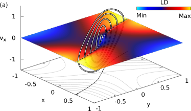
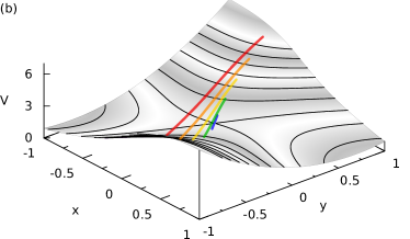
Figure 1: Visualization of five POs (solid lines) at different energies above the activation energy. Panel (a) shows an LD cut through phase space according to Eq. (1) with $\tau=10$ and a selection of POs in $(x,y,v_{x})$-space (analogous results are obtained also for $v_{y}$) and the LD is calculated for initial conditions $v_{x}=v_{y}=0$. The LD exhibits a minimum valley (dashed black and white lines) whose phase space coordinates belong to the periodic orbit at the respective energy. Panel (b) presents the configuration space projection of the POs together with the underlying potential. The POs presented have periods in the range $2.19\lesssim T\lesssim 2.45$, so that the integration time $\tau$ is sufficient to provide a high-resolution minimum LD valley.

In Fig. 1(a), we show a cut of the LD (1) through the $x$-$y$-plane in phase space for an integration time $\tau=10$ as a colored contour plot. (The selected value of $\tau$ is large compared to the periods $T$ of the POs shown in the figure which satisfy $2.19\lesssim T\lesssim 2.45$.) For each energy $E$ there are two minima of the LD which correspond to the intersection of the PO with that plane. All the minima of the LD at different energies together form a valley which is highlighted by the dashed white line. According to Eq. (4), each point on this line is an initial condition of a PO at the respective energy. Five POs selected at representative distinct energies $E>E^{\ddagger}$ are shown in $x$-$y$-$v_{x}$-space with little loss of information because $v_{y}$ is not shown. All five intersect with the $x$-$y$-plane at the LD’s minimum valley as suggested by Eq. (4). Figure 1(b) shows the configuration space projection of the POs together with the potential (5) visualizing the location of the POs on the potential energy surface.

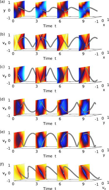
Figure 2: Complete time-dependent phase space representation of a periodic orbit (solid line) and the corresponding LD (1). The comparison shows that the PO’s coordinates are equivalent to the LD minimum throughout. The panels (a)–(f) show the time-evolution of both these objects for the different two-variable combinations of the variables $x,y,v_{x},v_{y}$.

A complete phase space visualization of the dynamics and LD of a single PO is shown in Fig. 2. Each panel shows the projection of the trajectory onto two of the four phase space variables. The trajectory is shown as a solid curve. A series of four colored contour planes of the LD is shown at selected times.

The PO intersects with all phase space cuts exactly where the LD minimum is located, once again verifying the relation in Eq. (4). Thus, the dynamical picture in Fig. 2 illustrates that this relation is valid in the whole phase space and for any time $t$.

III.2 Determining instanton trajectories in 2D

We now demonstrate the use of the LD-PO method for constructing instanton trajectories through a barrier. The instanton trajectory is a PO in the inverted potential $-V$ and, in a path integral formalism, it is directly related to the tunneling of a particle through the barrier.Miller (1974b, 1975b); Kleinert (2009); Stoof (1997); Wunner et al. (2008)

We use the potential

$$\begin{split}V(x,y)=&\frac{1}{2x^{2}}+\frac{1}{8y^{2}}+2\gamma_{x}^{2}x^{2}+2\gamma_{y}^{2}y^{2}+\frac{a}{2\sqrt{2}x^{2}y}\\ &+\frac{1+\kappa^{2}-(3x^{2}\arctan\sqrt{\eta})/(2y^{2}\sqrt{\eta})}{12\sqrt{2\pi}x^{2}y\eta}\,,\end{split}$$ (6)

where $\kappa=(x/y)^{2}$, $\eta=\kappa/2-1$, and $\gamma_{x,y},a$ are free parameters in arbitrary units. This potential describes within a mean-field approximation and a Gaussian approach to the wave function a dipolar Bose-Einstein condensate (BEC) in an axisymmetric, harmonic trap, where the variables $x,y$ can be interpreted as the mean extensions of the wave function.Huepe et al. (1999, 2003) The parameters $\gamma_{x,y}$ are the strength of the external traps (which we define by $\gamma_{x}^{2}\gamma_{y}=34\,000$ and $\gamma_{y}/\gamma_{x}=6$) and $a=0.1$ is the s-wave scattering length describing the contact interaction of two bosons. The physical meaning of Eq. (6) is as follows: The potential exhibits a local minimum at $x\approx 0.013$ and $y\approx 0.023$ which corresponds to the metastable ground state of the BEC and it diverges to $V\to-\infty$ for $x\to 0$. Both these regions are separated by a barrier and its crossing physically means the collapse of the BEC. There are two different ways to reach the collapsed state: One is the classical crossing of the barrier at high energies which is referred to as the thermally induced coherent collapse of the condensate.Huepe et al. (1999, 2003); Junginger et al. (2012); A. Junginger et al. (2013) The other possibility is the tunneling through the barrier in the limit of zero temperature referred to as macroscopic quantum tunneling.Stoof (1997); Wunner et al. (2008) As mentioned above, the theoretical description of the tunneling through the barrier in a path integral formalism Kleinert (2009) is directly related to the properties of the instanton trajectory which is the corresponding PO at the saddle of the inverted potential $-V$. In the following, we therefore apply the method described in Sec. II to those trajectories.

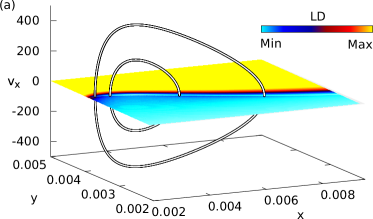
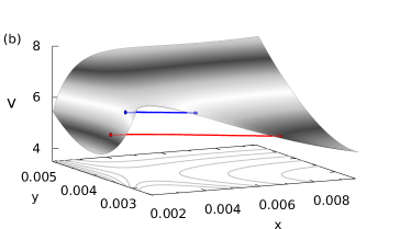
Figure 3: Visualization of two POs (solid lines) at different energies below the activation energy on the inverted potential $-V$ of Eq. (6): (a) A colored contour surface of LD values obtained at $\tau=10$ with POs cutting through the minimum values. (b) Configuration space projection of the instanton trajectories draw on the potential.

Figure 3(a) presents an LD cut through the $x$-$y$-plane calculated for the inverted potential, $-V$ in Eq. (6), and it can be seen that this LD portrait also exhibits a minimum valley. In analogy to the case in Sec. III.1, the corresponding phase space coordinates are initial values of classical POs in the inverted potential as indicated by the solid lines. The phase space coordinates at the minimum valley again correspond to initial points of the corresponding POs. We note here that, because of the divergence of the potential (6) for $x\to 0$, we have cut off the trajectories for the LD calculations when they have reached $x\leq 0.001$. This prevents one from facing numerical problems with the diverging potential for $x\to 0$, but it does not affect the search for the POs because they never reach this region.

Since the POs in Fig. 3(a) have been calculated for the inverted potential $-V$, the energy of the particles is below the saddle point energy for the real potential $+V$. In Fig. 3(b), we present the configuration space projection of the respective POs in the original potential $+V$, where the trajectories open up the tunnel connecting the two regions on both sides of the barrier.

IV Conclusion and outlook

From the relation of the PO being located at the intersection of the stable and unstable manifolds together with the fact that the LD exhibits extremal, i. e. minimal, values on these manifolds, we have presented a general construction scheme for this type of periodic orbits. Our LD-PO method is solely based on a minimization of the LD in phase space (or a subspace of constant energy, respectively). Neither boundary conditions nor any previous knowledge (e. g. the period $T$) are required. The procedure is easy to implement formally, as well as numerically, because the LD can be obtained on the fly when the trajectory is integrated and the minimization can be performed e. g. using standard algorithms.Press et al. (2007) Since the LD-PO method is based on minimizing a scalar phase space function, it can also be applied directly in higher-dimensional systems.

We have shown the applicability of the procedure to both the cases of energies above the saddle point, i. e. classical POs, as well as energies below the saddle point where the solutions represent the instanton trajectory related to the tunneling through the barrier. In both cases, we have identified minimum valleys of the LD in phase space which provide initial values of the POs at the respective energies.

We further observe that not only 1-cycles, but also $n$-cycles, can be obtained by the LD-PO method. Such POs of higher order emerge as local minima of the LD. They can be distinguished from each other by the LD’s actual value which is a measure of the PO’s cycle order. Possible applications lie in the general construction of POs in various systems and the extraction of periodic orbit dividing surfaces or instanton trajectories in reaction dynamics.