The recovery of a recessive allele
in a Mendelian diploid model

Abstract.

We study the large population limit of a stochastic individual-based model which describes the time evolution of a diploid hermaphroditic population reproducing according to Mendelian rules. In [27] it is proved that sexual reproduction allows unfit alleles to survive in individuals with mixed genotype much longer than they would in populations reproducing asexually. In the present paper we prove that this indeed opens the possibility that individuals with a pure genotype can reinvade in the population after the appearance of further mutations. We thus expose a rigorous description of a mechanism by which a recessive allele can re-emerge in a population. This can be seen as a statement of genetic robustness exhibited by diploid populations performing sexual reproduction.

1. Introduction

In population genetics, the study of Mendelian diploid models of fixed population size began more than a century ago (see e.g. [30, 16, 29, 18, 19, 12, 26, 15, 3]), while their counterparts of variable population size models were studied in the context of adaptive dynamics from 1999 onwards [22]. The approach of adaptive dynamics is to introduce competition kernels to regulate the population size instead of maintaining it constant, see [21, 23, 24].

Stochastic individual-based versions of these models appeared in the 1990s, see [13, 5, 4, 17, 6, 7]. They assume single events of reproduction, mutation, natural death, and death by competition happen at random times to each individual in the population. An important and interesting feature of these models is that different limiting processes on different time-scales appear as the carrying capacity tends to infinity while mutation rates and mutation step-size tend to zero (see [4, 13, 25, 7, 1]). One of the major results in this context is the convergence of a properly rescaled process to the so called Trait Substitution Sequence (TSS) process, which describes the evolution of a monomorphic population as a jump process between monomorphic equilibria. More generally, Champagnat and Méléard [7] obtained the convergence to a Polymorphic Evolution Sequence (PES), where jumps occur between equilibria that may include populations that have multiple co-existing phenotypes. The appearance of co-existing phenotypes is, however, exceptional and happens only at so-called evolutionary singularities. From a biological point of view, this is somewhat unsatisfactory, as it apparently fails to explain the biodiversity seen in real biological systems.

Most of the models considered in this context assume haploid populations with a-sexual reproduction. Exceptions are the paper [8] by Collet, Méléard and Metz from 2013 and a series of papers by Coron and co-authors [11, 9, 10] following it. In [8], the Trait Substitution Sequence is derived in a Mendelian diploid model under the assumption that the fitter mutant allele and the resident allele are co-dominant.

The main reason why both in haploid models and in the model considered in [8] the evolution along monomorphic populations is typical is that the time scales for the fixation of a new trait and the extinction of the resident trait are the same (both of order $\ln K$) (unless some very special fine-tuning of parameters occurs that allows for co-existence). This precludes (at least in the rare mutation scenarios considered) that an initially less fit trait survives long enough for several new mutations to occur, creating a situation where this trait may become fit again and recover.

In a follow-up paper to [8], two of the present authors [27], it was shown that, if instead one assumes that the resident allele is recessive, the time to extinction of this allele is dramatically increased. This will be discussed in detail in Section 1.2 and paves the way for the appearance of a richer limiting process.

The general framework in [8] and [27] is the following. Each individual is characterised by a reproduction and death rate which depend on a phenotypic trait determined by its genotype, which here is determined by two alleles (e.g. $A$ and $a$) on one single locus. The evolution of the trait distribution of the three genotypes $aa,aA$ and $AA$ is studied under the action of (1) heredity, which transmits traits to new offsprings according to Mendelian rules, (2) mutation, which produces variations in the trait values in the population onto which selection is acting, and (3) competition for resources between individuals.

The paper [27] proves that sexual reproduction allows unfit alleles to survive in individuals with mixed genotype much longer than they would in populations reproducing asexually. This opens the possibility that while this allele is still alive in the population, the appearance of new mutants alters the fitness landscape in such a way that is favourable for this allele and allows it to reinvade in the population, leading to a new equilibrium with co-existing phenotypes. The goal of this paper is to rigorously prove that such a scenario indeed occurs under fairly natural assumptions.
Recently, Billiard and Smadi [2] considered related questions for haploid individuals (performing clonal reproduction). The authors show that a deleterious allele can reinvade after a new mutation, but the range of parameters allowing this behaviour is though very small.

1.1. The stochastic model

The individual-based microscopic Mendelian diploid model is a non-linear birth-and-death process. We consider a model for a population of a finite number of hermaphroditic individuals which reproduce sexually. Each individual $i$ is characterised by two alleles, $u_{1}^{i}u_{2}^{i}$, taken from some allele space $\mathcal{U}\subset{\mathbb{R}}$. These two alleles define the genotype of the individual $i$. We suppress parental effects, which means that we identify individuals with genotype $u_{1}u_{2}$ and $u_{2}u_{1}$. Each individual has a Mendelian reproduction rate with possible mutations and a natural death rate. Moreover, there is an additional death rate due to ecological competition with the other individuals in the population. Let

$f_{u_{1}u_{2}}\in{\mathbb{R}}_{+}$	be the per capita birth rate (fertility) of an individual with genotype
	$u_{1}u_{2}$,
$D_{u_{1}u_{2}}\in{\mathbb{R}}_{+}$	be the per capita natural death rate of an individual with genotype $u_{1}u_{2}$,
$K\in{\mathbb{N}}$	be the carrying capacity, a parameter which scales the population size,
$\frac{c_{u_{1}u_{2},v_{1}v_{2}}}{K}\in{\mathbb{R}}_{+}$	be the competition effect felt by an individual with genotype $u_{1}u_{2}$ from an individual of genotype $v_{1}v_{2}$,
$R_{u_{1}u_{2}}(v_{1}v_{2})\!\in\!\{0,\!1\}$	be the reproductive compatibility of the genotype $v_{1}v_{2}$ with $u_{1}u_{2}$,
$\mu_{K}\in{\mathbb{R}}_{+}$	be the mutation probability per birth event. Here it is independent of
	the genotype,
$m(u,dh)$	be the mutation law of a mutant allelic trait $u+h\in\mathcal{U}$, born from an individual with allelic trait $u$.

Scaling the competition function $c$ down by a factor $1/K$ amounts to scaling the population size to order $K$. We are interested in asymptotic results when $K$ is large. We assume rare mutations, i.e. $\mu_{K}\ll 1$. If a mutation occurs at a birth event, only one allele changes from $u$ to $u+h$ where $h$ is a random variable with law $m(u,dh)$.

At any time $t$, there is a finite number, $N_{t}$, of individuals, each with genotype in $\mathcal{U}^{2}$. We denote by $u_{1}^{1}(t)u_{2}^{1}(t),...,u_{1}^{N_{t}}(t)u_{2}^{N_{t}}(t)$ the genotypes of the population at time $t$. The population, $\nu_{t}$, at time $t$ is represented by the rescaled sum of Dirac measures on $\mathcal{U}^{2}$,

$$\nu_{t}=\frac{1}{K}\sum_{i=1}^{N_{t}}\delta_{u_{1}^{i}(t)u_{2}^{i}(t)}.$$ (1.1)

Formally, $\nu_{t}$ takes values in the set of re-scaled point measures

$$\mathcal{M}^{K}=\left\{\frac{1}{K}\sum_{i=1}^{n}\delta_{u_{1}^{i}u_{2}^{i}}\;\Big{|}\;n\geq 0,u_{1}^{1}u_{2}^{1},...,u_{1}^{n}u_{2}^{n}\in\mathcal{U}^{2}\right\},$$ (1.2)

on $\mathcal{U}^{2}$, equipped with the vague topology.

For a formal construction of the corresponding measure valued Markov process, see [27]. We just insist on the reproduction rate of an individual of genotype $u_{1}u_{2}$ with an individual of genotype $v_{1}v_{2}$, which takes the form $f_{u_{1}u_{2}}\frac{f_{v_{1}v_{2}}R_{u_{1}u_{2}}(v_{1}v_{2})}{K\langle\nu R_{u_{1}u_{2}},f\rangle}$, where $\nu R_{u_{1}u_{2}}$ is the population restricted to the pool of potential partners of an individual of genotype $u_{1}u_{2}$. At the individual level, this form of reproduction rate means that each individual of genotype $u_{1}u_{2}$ reproduces at a rate which depends on its genotype through its fertility $f_{u_{1}u_{2}}$; more precisely, it bears an exponentially distributed clock with parameter $f_{u_{1}u_{2}}$, and when this rings, it chooses a partner at random in the pool determined by the reproductive compatibility $R$, with a weight proportional to the fertility of the partner. The reproductive compatibility can for example be thought as a way of coding if two individuals are or not of the same species. Within a species, the reproduction rate of a pair of (compatible) individuals is given by the product of their fertilities.

We make the following Assumptions (A):

• The functions $f,D$ and $c$ are measurable and bounded, which means that there exist constants $\bar{f},\bar{D},\bar{c}<\infty$ such that for all $u_{1}u_{2},v_{1}v_{2}\in\mathcal{U}^{2}$,

  $$0\leq f_{u_{1}u_{2}}\leq\bar{f},\quad 0\leq D_{u_{1}u_{2}}\leq\bar{D}\quad\text{and}\quad 0\leq c_{u_{1}u_{2},v_{1}v_{2}}\leq\bar{c}.\vspace{0pt}$$ (1.3)

• There exists a constant $\underline{c}>0$ such that for all $u_{1}u_{2}\in\mathcal{U}^{2}$, $c_{u_{1}u_{2},u_{1}u_{2}}\geq\underline{c}$ and $f_{u_{1}u_{2}}-D_{u_{1}u_{2}}>0$,

• There exists a function, $\bar{m}:{\mathbb{R}}\rightarrow{\mathbb{R}}_{+}$, such that $\int\bar{m}(h)dh<\infty$ and $m(u,h)\leq\bar{m}(h)$ for any $u\in\mathcal{U}$ and $h\in{\mathbb{R}}$.

For fixed $K$, under the Assumptions (A1)+(A3) and assuming that ${\mathbb{E}}(\langle\nu_{0},\mathbbm{1}\rangle)<\infty$, Fournier and Méléard [17] have shown existence and uniqueness in law of the process. For $K\rightarrow\infty$, under mild restrictive assumptions, they prove the convergence of the process in the space $\mathbb{D}({\mathbb{R}}_{+},\mathcal{M}^{K})$ of càdlàg functions from ${\mathbb{R}}^{+}$ to $\mathcal{M}_{K}$, to a deterministic process, which is the solution to a non-linear integro-differential equation. Assumption (A2) ensures that the population does not tend to infinity in finite time or becomes extinct too fast.

1.2. Previous works

Consider the process starting with a monomorphic $aa$ population, with one additional mutant individual of genotype $aA$. Assume that the phenotype difference between the mutant and the resident population is small. The phenotype difference is assumed to be a slightly smaller death rate compared to the resident population, namely

$$D_{aa}=D,\quad D_{aA}=D-\Delta,$$ (1.4)

for some small enough $\Delta>0$. The mutation probability for an individual with genotype $u_{1}u_{2}$ is given by $\mu_{K}$. Hence, the time until the next mutation in the whole population is of order $\frac{1}{K\mu_{K}}$. Now assume that the demographic parameters introduced in Section 1.1 depend continuously on the phenotype. In particular, they are the same for individuals bearing the same phenotype.

In [8] it is proved that if the two alleles $a$ and $A$ are co-dominant and if the allele $A$ is slightly fitter than the allele $a$, namely

$$D_{aa}=D,\quad D_{aA}=D-\Delta,\quad D_{AA}=D-2\Delta,$$ (1.5)

then in the limit of large population and rare mutations ($\ln K\ll\frac{1}{\mu_{K}K}\ll e^{VK}$ for some $V>0$), the suitably time-rescaled process converges to the TSS model of adaptive dynamics, essentially as shown in [4] in the haploid case. In particular, the genotypes containing the unfit allele $a$ decay exponentially fast after the invasion of $AA$ (see Figure 1).

If in place of co-dominance we assume, as in [27], that the fittest phenotype $A$ is dominant, namely

$$D_{aa}=D,\quad D_{aA}=D-\Delta,\quad D_{AA}=D-\Delta,$$ (1.6)

then this has a dramatic effect on the evolution of the population and, in particular, leads to a much prolonged survival of the unfit phenotype $aa$. Indeed, it was known for some time (see e.g. [26]) that in this case the unique stable fixed point $(0,0,\bar{n}_{AA})$ corresponding to a monomorphic $AA$ population is degenerate, i.e. its Jacobian matrix has zero-eigenvalue. This implies that in the deterministic system, the $aa$ and $aA$ populations decay in time only polynomially fast to zero, namely like $1/t^{2}$ and $1/t$, respectively. This is in contrast to the exponential decay in the co-dominant scenario (see Figure 1). In [27] it was shown that the deterministic system remains a good approximation of the stochastic system as long as the size of the $aA$ population remains much larger than $K^{1/2}$ and therefore that the $a$ allele survives for a time of order at least $K^{1/2-{\alpha}}$, for any ${\alpha}>0$. Note that this statement is a non trivial fact, since it is not a consequence of the law of large numbers, because the time window diverges as $K$ grows. In summary, the unfit recessive $a$ allele survives in the population much longer due to the slow decay of the $aA$ population.

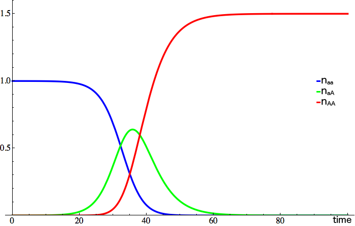
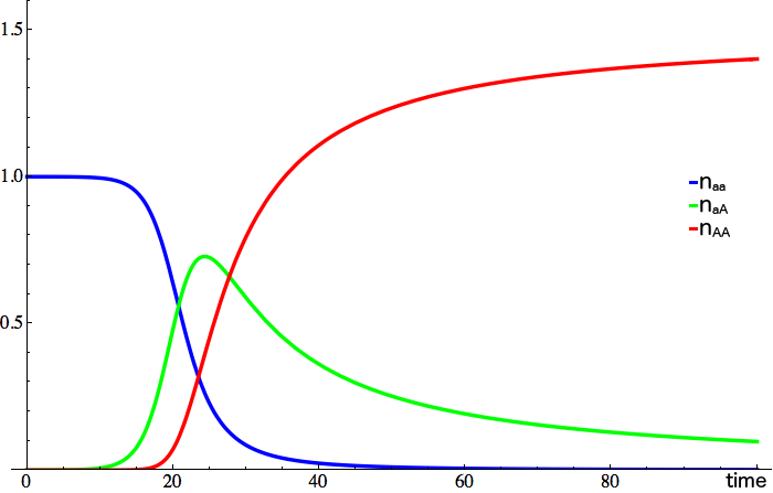
Figure 1. Evolution of the model from a resident $aa$ population at equilibrium with a small amount of mutant $aA$, and when the alleles $a$ and $A$ are co-dominant (left) or when the mutant phenotype $A$ is dominant (right).

It is argued in [27] that if we choose the mutation time scale in such a way that there remain enough $a$ alleles in the population when a new mutation occurs, i.e.

$$\ln K\ll\frac{1}{\mu_{K}K}\ll K^{1/2-\alpha}\quad\text{as }K\to\infty,\text{for some }\alpha>0,$$ (1.7)

and if the new mutant can coexist with the unfit $aa$ individuals, then the $aa$ population can potentially recover. This is the starting point of the present paper.

1.3. Goal of the paper

The goal of this paper is to show that under reasonable hypotheses, the prolonged survival of the $a$ allele after the invasion of the $A$ allele can indeed lead to a recovery of the $aa$-type. To do this, we assume that there will occur a new mutant allele (on the same gene), $B$, that on the one hand has a higher fitness than the $AA$-phenotype but that (for simplicity) has no competition with the $aa$-type. The possible genotypes after this mutation are $aa,aA,AA,aB,AB$, and $BB$, so that even for the deterministic system we have now to deal with a $6$-dimensional dynamical system whose analysis if far from simple.

Under the assumption of dominance of the fittest phenotype, and mutation rate satisfying (1.7), we consider the model described in Section 1.1 starting at the time of the second mutation, that is (with probability converging to 1 as $K\to\infty$) the $AA$ population being close to its equilibrium and the $aA$ population having decreased to a size of order ${\varepsilon}_{K}=O(K\mu_{K})$, while the $aa$ population is of the order of the square of the $aA$ population. We assume that there just occurred a mutation to a fitter (and more dominant) allele $B$: we thus start with a quantity $\frac{1}{K}$ of genotype $AB$. We will start with a population where $AA$ is close to its equilibrium, the populations of $aA$ and $aa$ are already small (of order ${\varepsilon}_{K}$ and ${\varepsilon}_{K}^{2}$), and by mutation a single individual of genotype $AB$ appears.

By using well known techniques [4, 7, 8], we know that the $AB$ population behaves as a super-critical branching process and reaches a level ${\varepsilon}_{0}>0$ with positive probability in a time of order $\ln K$, without perturbing the 3-system $(aa,aA,AA)$.

We see in numerical solutions to the deterministic system that a reduced fertility together with a reduced competition between $a$ and $B$ phenotypes constitutes a sufficient condition for the recovery of the $aa$ population. For simplicity and in order to prove rigorous results, we suppose that there can be no reproduction between individuals of phenotypes $a$ and $B$, nor competition between them, and we reduce the number of remaining parameters as much as possible (see Section 2). We study the deterministic system which corresponds to the large population limit of the stochastic counterpart, and we show that (for an initial quantity ${\varepsilon}$ of $aA$, ${\varepsilon}^{2}$ of $aa$ and ${\varepsilon}^{3}$ of $AB$) the system converges to a fixed point denoted by $p_{aB}$ consisting of the two coexisting populations $aa$ and $BB$. If no further assumptions are made, we show that the number of individuals bearing an $a$ allele decreases to level ${\varepsilon}^{1+{\Delta}/(1-{\Delta})}$ (where $\Delta$ is defined in (1.4)) before $aa$ grows and stabilises at order 1.

Remark.

Note that our study considers an initial quantity of $aA$ individuals $n_{aA}(0)={\varepsilon}>0$, which should be thought as ${\varepsilon}={\varepsilon}_{K}=O(K\mu_{K})$ for the following discussion about the associated stochastic system. The quantity ${\varepsilon}_{K}$ satisfies $(\ln K)^{-1}\ll{\varepsilon}_{K}\ll O(K^{-\frac{1}{2}+\alpha})$ if the mutation time satisfies (1.7).

Let us discuss the (conjectural) implications of our results on the stochastic system:
If $\Delta<\frac{\alpha}{1-2\alpha}$, our control on the $a$ allele is in principle sufficient in order for the stochastic system to exhibit the recovery of $aa$ with positive probability in the large population limit. Indeed, if the mutation time is of order $K^{\frac{1}{2}-\alpha}$, then the initial amount of $aA$ and $aa$ genotypes is close to the typical fluctuations of those populations, that is respectively of orders $O(K^{-\frac{1}{2}+\alpha})$ and $O(K^{-1+2\alpha})$. Following the heuristics of [27] (although the six-dimensional stochastic process is surely much more tedious to study), the deterministic system should constitute a good approximation of the process if the typical fluctuations of populations containing an $a$ allele do not bring them to extinction. If $\Delta<\frac{\alpha}{1-2\alpha}$ this ensures that the population containing an $a$ allele is not falling below order $K^{-1/2}$ at any time.

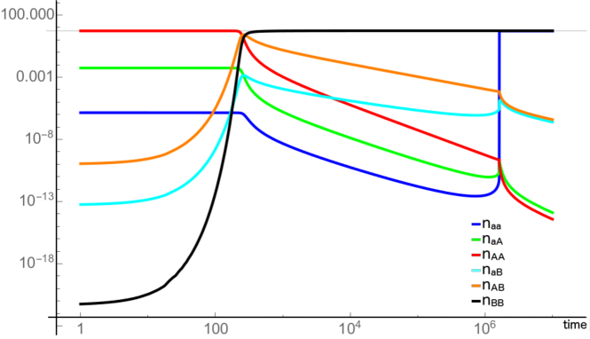
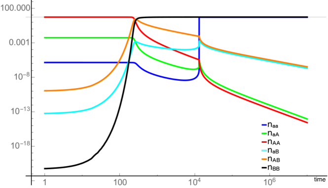
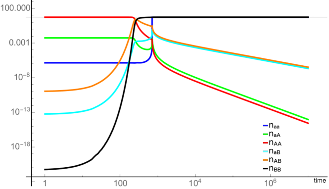
Figure 5. Log-plots of $\{n_{i}(t),i\in\mathcal{G}\}$ for $\eta=0$ (top), $\eta=0.003$ (center) and $\eta=0.014$ (bottom).

In order to go deeper and control the speed of recovery of the $aa$ population, we look for a parameter regime which ensures that the $aa$ population always grows after the invasion of $B$. Ensuring this lower bound on $aa$ is not trivial at all, and the solution we found is to introduce an additional parameter $\eta$, which lowers the competition between the $aA$ and $BB$ populations, compared to the one between $AA$ and $BB$. Note that the competition does not depend only on the phenotype, and can be interpreted as a refinement of a phenotypic competition for resources: the strength (or ability to get resources) of an individual not only depends on its phenotype but also on the dominance of its genotype. A biological interpretation for this kind of competition could be that it is coded in the alleles which food an individual with a given genotype prefers. We show that for $\eta$ larger than some positive value (of order $\Delta$), the $aa$ population always grows after the invasion of $B$. The time of convergence to the coexistence fixed point is thus lowered, see Figure 5. Moreover, we point out the existence of a bifurcation: for $\eta$ larger than some threshold, the co-existence fixed point $p_{aB}$ becomes unstable and the system converges to another fixed point where all populations coexist.

Our contribution is a rigorous description of a mechanism by which a recessive allele can re-emerge in a population. This can be seen as a statement of genetic robustness exhibited by diploid populations performing sexual reproduction.

The structure of the paper is the following. In Section 2 we describe our assumptions on the parameters of the model, and compute the large population limit; in Section 3 we present our results on the evolution of the deterministic system towards the co-existence fixed point $p_{aB}$, and we give a heuristic of the proof. Section 4 is dedicated to the proof of these results. The closing Section 5 contain a heuristic considerations and numerical simulations of the model with relaxed assumption on the parameters.

Figure 2. Simulation of the stochastic system for $f=6,D=0.7$, $\Delta=0.1$, $c=1,\eta=0.02$, ${\varepsilon}=0.014$ and $K=7000$.

Notation.

We write $x={\Theta}(y)$ whenever $x=O(y)$ and $y=O(x)$ as ${\varepsilon}\to 0.$

2. Model setup

Let $\mathcal{G}=\{aa,aA,AA,aB,AB,BB\}$ be the genotype space. Let $n_{i}(t)$ be the number of individuals with genotype $i\in\mathcal{G}$ in the population at time $t$ and set $n^{K}_{i}(t)\equiv\frac{1}{K}n_{i}(t)$.

Definition 2.1.

The equilibrium size of a monomorphic $uu$ population, $u\in\{a,A,B\}$, is the fixed point of a 1-dimensional Lotka-Volterra equation and is given by

$$\bar{n}_{u}=\frac{f_{uu}-D_{uu}}{c_{uu,uu}}.$$ (2.1)

Definition 2.2.

For $u,v\in\{a,A,B\}$, we call

$$S_{uv,uu}=f_{uv}-D_{uv}-c_{uv,uu}\bar{n}_{u},$$ (2.2)

the invasion fitness of a mutant $uv$ in a resident $uu$ population.

We take the phenotypic viewpoint and assume that the $B$ allele is the most dominant one. That means the ascending order of dominance (in the Mendelian sense) is given by $a<A<B$, i.e.

1. phenotype $a$ consists of the genotype $aa$,

2. phenotype $A$ consists of the genotypes $aA,AA$,

3. phenotype $B$ consists of the genotypes $aB,AB,BB$.
   

For simplicity, we assume that the fertilities are the same for all genotypes, and that natural death rates are the same within the three different phenotypes. Moreover, we assume that there can be no reproduction between $a$ and $B$ phenotypes.
To sumarize, we make the following Assumptions (B) on the rates:

• Fertilities. For all $i\in\mathcal{G}$, and some $f>0$

  $$f_{i}\equiv f.$$ (2.3)

• Natural death rates. The difference in fitness of the three phenotypes is realised by choosing a slightly higher natural death-rate of the $a$-phenotype and a slightly lower death-rate for the $B$-phenotype. For some $0<{\Delta}<D$,

  $$D_{aa} =D+{\Delta},$$ (2.4)

  $$D_{AA}\equiv D_{aA} =D,$$ (2.5)

  $$D_{aB}\equiv D_{AB}\equiv D_{BB} =D-{\Delta}.$$ (2.6)

• Competition rates. We require that phenotypes $a$ and $B$ do not compete with each other. Moreover, we introduce a parameter $\eta\geq 0$ which lowers the competition between $BB$ and $aA$. For some $0\leq\eta<c$,

  $$\left(c_{i,j}\right)_{\{i,j\}\in\mathcal{G}\times\mathcal{G}}=:\begin{tabular}[]{c|c|c|c}&$aa$&$aA\quad AA$&$aB\quad AB\quad BB$\\ \hline\cr$aa$&$c$&$c\quad c$&$0\quad 0\quad 0$\\ \hline\cr$aA$&$c$&$c\quad c$&$c\quad c\quad c-\eta$\\ $AA$&$c$&$c\quad c$&$c\quad c\quad c$\\ \hline\cr$aB$&$0$&$c\quad c$&$c\quad c\quad c$\\ $AB$&$0$&$c\quad c$&$c\quad c\quad c$\\ $BB$&$0$&$c-\eta\quad c$&$c\quad c\quad c$\\ \hline\cr\end{tabular}$$

  Remark.

  If $\eta>0$, the competition does not depend only on the phenotype, and can be interpreted as a refinement of a phenotypic competition for resources: the strength (or ability to get resources) of an individual not only depends on its phenotype but also on its genotype. Genetically, it makes sense to assume that (positive) competition rates are decreasing in the ”genetic distance” between two individuals. This is the case for the above competition matrix if we assume that the mutations $a\to A\to B$ can only occur successively. Indeed, the Hamming distance between genotypes is then the following graph distance, where $d(aA,BB)>d(AA,BB)$.

  

• Reproductive compatibility. We require that phenotypes $a$ and $B$ do not reproduce with each other.

  $$\left(R_{i}(j)\right)_{\{i,j\}\in\mathcal{G}\times\mathcal{G}}\equiv\begin{tabular}[]{c|c|c|c}&$aa$&$aA\quad AA$&$aB\quad AB\quad BB$\\ \hline\cr$aa$&$1$&$1\quad 1$&$0\quad 0\quad 0$\\ \hline\cr$aA$&$1$&$1\quad 1$&$1\quad 1\quad 1$\\ $AA$&$1$&$1\quad 1$&$1\quad 1\quad 1$\\ \hline\cr$aB$&$0$&$1\quad 1$&$1\quad 1\quad 1$\\ $AB$&$0$&$1\quad 1$&$1\quad 1\quad 1$\\ $BB$&$0$&$1\quad 1$&$1\quad 1\quad 1$\\ \hline\cr\end{tabular}$$

Observe that, under Assumptions (B),

$$S_{AB,AA} =f-(D-{\Delta})-c\bar{n}_{AA}=f-D+\Delta-c\frac{f-D}{c}={\Delta},$$ (2.7)

$$S_{aa,BB} =f-D-{\Delta},$$ (2.8)

$$c\bar{n}_{B} =f-D+\Delta$$ (2.9)

Therefore, the mutant $AB$ has a positive invasion fitness in the population $AA$, as well as $aa$ in the $BB$ population (due to the absence of competition between them).

2.1. Birth rates

Since we assume that there is no recombination between phenotypes $a$ and $B$. Thus,

1. the pool of possible partners for the phenotype $a$ consists of phenotypes $a$ and $A$; the total population of this pool is denoted by

   $$\Sigma_{3}:=n_{aa}+n_{aA}+n_{AA},$$ (2.10)

2. the pool of possible partners for the phenotype $A$ consists of the three phenotypes $a$, $A$, and $B$; the total population of this pool is denoted by

   $$\Sigma_{6}:=n_{aa}+n_{aA}+n_{AA}+n_{aB}+n_{AB}+n_{BB},$$ (2.11)

3. the pool of possible partners for the phenotype $B$ consists of phenotypes $A$ and $B$; the total population of this pool is denoted by

   $$\Sigma_{5}:=n_{aA}+n_{AA}+n_{aB}+n_{AB}+n_{BB}.$$ (2.12)

Computing the reproduction rates with the Mendelian rules as described in [27] leads to the following (time-dependent) birth-rates $b_{i}=b_{i}(n(t))$:

$$b_{aa}= f\frac{n_{aa}\left(n_{aa}+\frac{1}{2}n_{aA}\right)}{\Sigma_{3}}+f\frac{\frac{1}{2}n_{aB}\left(\frac{1}{2}n_{aA}+\frac{1}{2}n_{aB}\right)}{\Sigma_{5}}+f\frac{\frac{1}{2}n_{aA}\left(n_{aa}+\frac{1}{2}n_{aA}+\frac{1}{2}n_{aB}\right)}{\Sigma_{6}},$$ (2.13)

$$b_{aA}= f\frac{n_{aa}\left({\textstyle{1\over 2}}n_{aA}+n_{AA}\right)}{\Sigma_{3}}+f\frac{\frac{1}{2}n_{aA}\left(\frac{1}{2}n_{aB}+\frac{1}{2}n_{AB}\right)+\frac{1}{2}n_{aB}\left(n_{AA}+n_{AB}\right)}{\Sigma_{5}}$$

$$+f\frac{\left(\frac{1}{2}n_{aA}+n_{AA}\right)\left(n_{aa}+n_{aA}+\frac{1}{2}n_{aB}\right)+\frac{1}{4}n_{aA}n_{AB}}{\Sigma_{6}},$$ (2.14)

$$b_{AA}= f\frac{\frac{1}{2}n_{AB}\left(\frac{1}{2}n_{aA}+n_{AA}+\frac{1}{2}n_{AB}\right)}{\Sigma_{5}}+f\frac{\left(\frac{1}{2}n_{aA}+n_{AA}\right)\left(\frac{1}{2}n_{aA}+n_{AA}+\frac{1}{2}n_{AB}\right)}{\Sigma_{6}},$$ (2.15)

$$b_{aB}= f\frac{\left(\frac{1}{2}n_{aA}+n_{aB}\right)\left(\frac{1}{2}n_{aB}+\frac{1}{2}n_{AB}+n_{BB}\right)}{\Sigma_{5}}+f\frac{\frac{1}{2}n_{aA}\left(\frac{1}{2}n_{aB}+\frac{1}{2}n_{AB}+n_{BB}\right)}{\Sigma_{6}},$$ (2.16)

$$b_{AB}= f\frac{\left(\frac{1}{2}n_{aA}+n_{AA}+n_{AB}\right)\left(\frac{1}{2}n_{aB}+\frac{1}{2}n_{AB}+n_{BB}\right)}{\Sigma_{5}}+f\frac{\left(\frac{1}{2}n_{aA}+n_{AA}\right)\left(\frac{1}{2}n_{aB}+\frac{1}{2}n_{AB}+n_{BB}\right)}{\Sigma_{6}},$$ (2.17)

$$b_{BB}= f\frac{\frac{1}{4}\left(n_{aB}+n_{AB}+2n_{BB}\right)^{2}}{\Sigma_{5}}.$$ (2.18)

2.2. Death rates

The death rates are the sum of the natural and competition death rates:

$$d_{aa} =n_{aa}(D+{\Delta}+c\Sigma_{3}),$$ (2.19)

$$d_{aA} =n_{aA}(D+c(n_{aa}+n_{aA}+n_{AA}+n_{aB}+n_{AB})+(c-\eta)n_{BB}),$$ (2.20)

$$d_{AA} =n_{AA}(D+c\Sigma_{6}),$$ (2.21)

$$d_{aB} =n_{aB}(D-{\Delta}+c\Sigma_{5}),$$ (2.22)

$$d_{AB} =n_{AB}(D-{\Delta}+c\Sigma_{5}),$$ (2.23)

$$d_{BB} =n_{BB}(D-{\Delta}+(c-\eta)n_{aA}+c(n_{AA}+n_{aB}+n_{AB}+n_{BB})).$$ (2.24)

2.3. Large population limit

By [17] or [8], for large populations, the behaviour of the stochastic process is close to the solution of a deterministic equation.

Proposition 2.3 (Theorem 2.1 in [14]).

Let $T>0$ and $C\subset{\mathbb{R}}_{+}^{6}$ be a compact set. Assume that the initial condition $n^{K}(0)=\frac{1}{K}(n_{aa}(0),n_{aA}(0),n_{AA}(0),n_{aB}(0),n_{AB}(0),n_{BB}(0))$ converges almost surely to a deterministic vector $x^{0}=(x^{0}_{1},x^{0}_{2},x^{0}_{3},x^{0}_{4},x^{0}_{5},x^{0}_{6})\in C$, as $K\to\infty$.
Let $\tilde{n}(t,x^{0})$ denote the solution to

$$\dot{n}(t) =b(n(t))-d(n(t))\equiv F(n(t)),$$ (2.25)

$$\hbox{\rm i.e.}\quad\dot{n}_{i}(t) =b_{i}(n(t))-\left(D_{i}+\sum_{j\in{\mathcal{G}}}c_{i,j}n_{j}(t)\right)n_{i}(t),\quad\text{for all }i\in{\mathcal{G}},$$ (2.26)

with initial condition $x^{0}$, where $(b_{i})_{i\in{\mathcal{G}}}$ and $(d_{i})_{i\in{\mathcal{G}}}$ are given in (2.13)-(2.18) and (2.19)-(2.24). Then, for all $T>0$,

$$\lim_{K\rightarrow\infty}\sup_{t\in[0,T]}|n^{K}_{i}(t)-\tilde{n}_{i}(t,x^{0}))|=0,\quad\text{a.s.},$$ (2.27)

for all $i\in{\mathcal{G}}$.

2.4. Initial condition

Fix ${\varepsilon}>0$ sufficiently small. For the results below, we will consider the dynamical system (2.25) starting with the initial condition:

$$\bar{n}_{A}\geq n_{AA}(0) \geq\bar{n}_{A}-{\Theta}({\varepsilon}),$$ (2.28)

$$n_{aA}(0) ={\varepsilon},$$ (2.29)

$${\varepsilon}^{2}\geq n_{aa}(0) ={\Theta}({\varepsilon}^{2}),$$ (2.30)

$$n_{AB}(0) ={\varepsilon}^{3},$$ (2.31)

$$n_{BB}(0) =0,$$ (2.32)

$$n_{aB}(0) =0,$$ (2.33)

which corresponds to the long time behaviour of the dynamical system considered in [27] plus a quantity ${\varepsilon}^{3}$ of the new mutant $AB$.

Remark.

In all the figures below, the choice of parameters is the following:

$f=6$,

$D=0.7$,

$\Delta=0.1$,

$c=1$,

${\varepsilon}=0.01$,

and the parameter $\eta$ is specified on each picture.

3. Results

We are working with a 6-dimensional dynamical system, and computing all the fixed points analytically is impossible for a general choice of the parameters. We can, however, compute those which are relevant for our study. We will call $p_{A}$ (resp. $p_{B}$) the fixed points corresponding to the monomorphic $AA$ (resp. $BB$) population at equilibrium, and $p_{aB}$ the fixed point corresponding to the coexisting $aa$ and $BB$ populations. Setting the relevant populations to 0 and solving $\dot{n}(t)=0$, we get:

$$p_{A} =(0,0,\bar{n}_{A},0,0,0),$$ (3.1)

$$p_{B} =(0,0,0,0,0,\bar{n}_{B}),$$ (3.2)

$$p_{aB} =(\bar{n}_{a},0,0,0,0,\bar{n}_{B}),$$ (3.3)

where $\bar{n}_{a}=\frac{f-D-\Delta}{c},\bar{n}_{A}=\frac{f-D}{c},$ and $\bar{n}_{B}=\frac{f-D+\Delta}{c}.$ Note that the $BB$ equilibrium population is the same in $p_{B}$ and $p_{aB}$. This is due to the non-interaction between phenotypes $a$ and $B$.

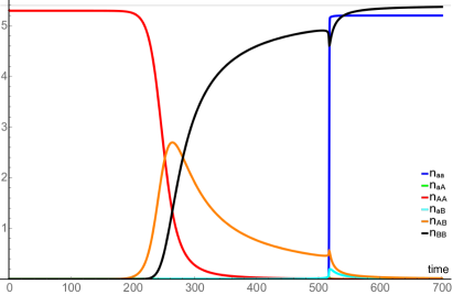
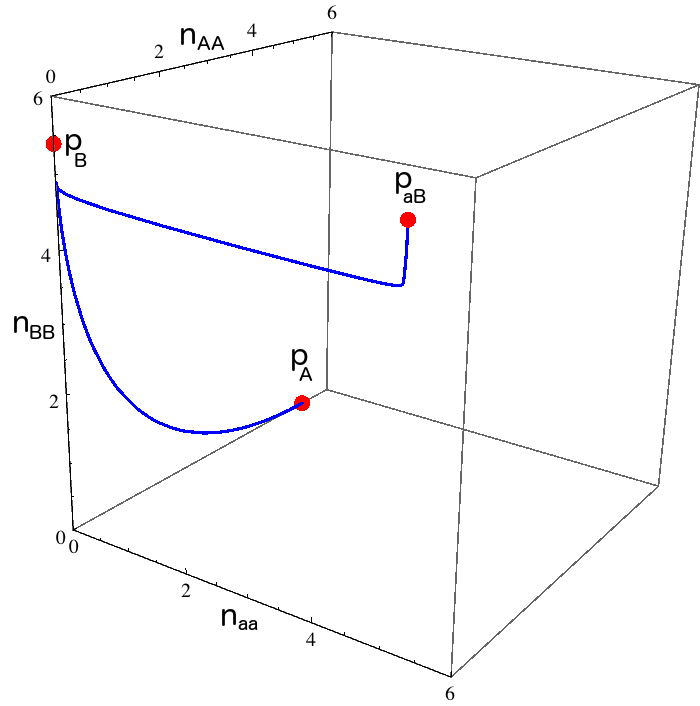
Figure 3. General qualitative behaviour of $\{n_{i}(t),i\in\mathcal{G}\}$ and projection of the dynamical system on the coordinates $aa,AA$ and $BB$. The re-invasion of the $aa$ population happens sooner and sooner as $\eta$ grows ($\eta=0.02$ for both pictures).

Our general result is that starting with initial conditions (2.28)-(2.33), that is close to $p_{A}$ (with small coordinates in directions $aa$, $aA$ and $AB$), and under minimal assumptions on the parameters, the system gets very close to $p_{B}$ before finally converging to $p_{aB}$, see Figure 3.

Theorem 3.1.

Consider the dynamical system (2.25) started with initial conditions (2.28)-(2.33). Suppose the following Assumptions (C) on the parameters hold:

1. $\Delta$ sufficiently small,

2. $f$ sufficiently large,

3. $0\leq\eta<c/2$.

Then the system converges to the fixed point $p_{aB}$. More precisely, for any fixed $\delta>0$, as ${\varepsilon}\to 0$, it reaches a $\delta$-neighbourhood of $p_{aB}$ in a time of order ${\Theta}({\varepsilon}^{-1/(1+\eta\bar{n}_{B}-{\Delta})})$.
Moreover:

1. for $\eta=0$, the amount of allele $a$ in the population decays to ${\Theta}({\varepsilon}^{1+{\Delta}/(1+{\Delta})})$ before reaching ${\Theta}(1)$,

2. for $\eta>\frac{4{\Delta}}{\bar{n}_{B}}$, the amount of $a$ allele in the population is bounded below by ${\Theta}({\varepsilon})$ for all $t>0$.

Remark.

For $\eta$ large, we prove that the fixed point $p_{aB}$ is unstable. We observe numerically that the system is attracted to a fixed point where all the 6 populations coexist, but we do not prove this.

Let us now briefly discuss the linear stability of the relevant fixed points and give a heuristics of the proof of Theorem 3.1.

3.1. Linear stability analysis

The Jacobian matrix $J_{F}:=(\partial F_{i}/\partial n_{j})_{ij}$ of the map $F$ defined in (2.25) can be explicitly computed at $p_{A}$ and $p_{aB}$ and the situation is as follows:

• The eigenvalues of $J_{F}(p_{A})$ are $0,\Delta>0$ and $-(f-D),-(f+\Delta),-(f-\Delta)$ (double) which are all strictly negative under Assumptions (C). The fixed point $p_{A}$ is thus unstable.

• The eigenvalues of $J_{F}(p_{aB})$ are $0$ (double), and $-(2f-D),-(f-D+\Delta),-(f-D-\Delta),-((f-D)(5f-4D)+f\Delta)/(4(f-D)+\eta\bar{n}_{B})$ which are strictly negative under Assumptions (C). The linear analysis thus does not imply the stability of $p_{aB}$ but the Phase 4 of the proof does (see Section 4.5) .

It turns out that $J_{F}(p_{B})$ is singular but as the invasion fitness of $aa$ is positive, i.e. $S_{aa,BB}>0$ (see (2.7)), this implies that a small perturbation in the first coordinate will be amplified, and thus implies the instability of the fixed point $p_{B}$.

3.2. Heuristics of the proof

Recall we start the dynamical system (2.25) with initial conditions (2.28)-(2.33). A numerical solution of the system is provided on Figure 4.

Remark.

Assumption C1 of Theorem 3.1 is needed throughout the proof in order to be able to use the results of [27] which rely on the Center Manifold Theorem (a line of fixed points becomes an invariant line under small enough perturbation).

1. Time period: until $n_{AB}={\varepsilon}_{0}$.
   The mutant population, consisting of all individuals of phenotype $B$, first grows up to ${\varepsilon}_{0}$ exponentially fast with rate $\Delta$ without perturbing the behaviour of the 3-system $(aa,aA,AA)$. The rate of growth corresponds to the invasion fitness of $AB$ in the resident population $AA$, see (2.7). Following [27], $AA$ stays close to $\bar{n}_{A}$, while $aA$ and $aa$ continue to decay like $1/t$ and $1/t^{2}$ respectively. The duration $T_{1}$ of this phase is such that ${\Theta}({\varepsilon}^{3})e^{t{\Delta}}={\Theta}(1)\Leftrightarrow T_{1}={\Theta}(|\log{\varepsilon}|)$.
   

2. Time period: until $n_{aA}={\Theta}(n_{AA})$.
   The evolution is a perturbation of an effective 3-system $(AA,AB,BB)$ which behaves exactly the same as in [27], since the parameters satisfy the same hypotheses (slightly lower death rate for phenotype $B$ than for phenotype $A$, and constant competition parameters). A comparison result (following Theorem 4.6 below) shows that this 3-system is almost unperturbed until $n_{aA}={\Theta}(n_{AA})$. If that happens in a time $T_{2}$ diverging with ${\varepsilon}$ (which we ensure throughout the calculation), we thus know that $BB$ approaches $\bar{n}_{B}$, while $n_{AB}\propto 1/t$ and $n_{AA}\propto 1/t^{2}$.
   The important fact in this phase is that the amount of allele $a$ in the population decays for $\eta$ small while it increases for large enough $\eta$. Indeed, let us derive some bounds on $\Sigma_{aA,aB}=n_{aA}+n_{aB}$. The population $\Sigma_{aA,aB}$ reproduces by taking the dominant allele in a population of order ${\Theta}(1)$ and the allele $a$ in itself. Thus its birth rate satisfies $b_{\Sigma_{aA,aB}}\approx f\Sigma_{aA,aB}$. We can compute its death rate exactly and use that $n_{BB}\approx\Sigma_{5}\approx\bar{n}_{B}$:

   $$d_{\Sigma_{aA,aB}} =\Sigma_{aA,aB}(D-{\Delta}+c\Sigma_{5})-\eta n_{aA}n_{BB}+{\Delta}n_{aA}$$

   $$\approx f\Sigma_{aA,aB}-n_{aA}(\eta\bar{n}_{B}-{\Delta}),$$ (3.4)

   $$\dot{\Sigma}_{aA,aB} \approx n_{aA}(\eta\bar{n}_{B}-{\Delta})$$

   $$={\Theta}({\Sigma}_{aA,aB}\cdot n_{AB})(\eta\bar{n}_{B}-{\Delta}).$$ (3.5)

   The last equality comes from the fact that $aA$ newborns have mainly their $a$ allele coming from ${\Sigma}_{aA,aB}$ and their $A$ allele coming from $AB$. Using the $1/t$ decay of $AB$ we get:

   $$\dot{\Sigma}_{aA,aB}\approx\frac{{\Theta}({\Sigma}_{aA,aB})}{{\Theta}(1)+{\Theta}(1)t}(\eta\bar{n}_{B}-{\Delta})$$ (3.6)

   As ${\Sigma}_{aA,aB}(T_{1})={\Theta}({\varepsilon})$ we deduce that ${\Sigma}_{aA,aB}(t)={{\Theta}({\varepsilon})}({\Theta}(1)+{\Theta}(1)t)^{{\Theta}(\eta\bar{n}_{B}-{\Delta})}$, and thus $n_{aA}={\Theta}(n_{AB}\cdot{\Sigma}_{aA,aB})={{{\Theta}({\varepsilon})}({\Theta}(1)+{\Theta}(1)t)^{{\Theta}(\eta\bar{n}_{B}-{\Delta})}}/{({\Theta}(1)+{\Theta}(1)t)}$. By solving $n_{aA}={\Theta}(n_{AA})={\Theta}(n_{AB}^{2})$ we get the order of magnitude of $T_{2}={\Theta}\left({\varepsilon}^{-1/(1+\eta\bar{n}_{B}-{\Delta})}\right)$. Note that for $\eta=0$, ${\Sigma}_{aA,aB}(T_{2})={\Theta}({\varepsilon}^{1+{{\Delta}}/{(1-{\Delta})}})$. Moreover, (3.5) implies that for $\eta>\Delta/\bar{n}_{B}$, we have $\dot{\Sigma}_{aA,aB}>0$, which proves points 1 and 2 of Theorem 3.1.
   

3. Time period: until ${aa}$ reaches equilibrium.
   The fact that $n_{aA}={\Theta}(n_{AA})$ has a crucial effect on the birth rate of $aa$ (see (2.13)) since the term $(n_{aa}+\frac{1}{2}n_{aA})/({n_{aa}+n_{aA}+n_{AA}})$ becomes of order ${\Theta}(1)$. As long as $AA$ stays smaller than ${\Theta}({\varepsilon})$, we get a lower bound on $n_{aa}$ which grows exponentially fast since $f$ is chosen large enough (Assumption C2):

   $$b_{aa} \geq fn_{aa}{\Theta}(1),$$ (3.7)

   $$d_{aa} \leq n_{aa}(D+{\Delta}+{\Theta}({\varepsilon})),$$ (3.8)

   $$\dot{n}_{aa} \geq n_{aa}(f{\Theta}(1)-D-{\Delta}-{\Theta}({\varepsilon})).$$ (3.9)

   As $aa$ grows, it makes ${\Sigma}_{aA,aB}$ grow, and thus $AA$ and $AB$ as well. We have to show that this could not prevent $aa$ from reaching equilibrium. We do not give a detailed argument here, but essentially, the presence of the macroscopic $BB$ population prevents all the non-$aa$ populations to grow too much. Note that if $\eta$ is too large, then $aA$ could get a positive fitness and grow to a macroscopic level. That is why we have to impose Assumption C3, which will become clearer heuristically in the next phase. We recall that $aa$ does not compete with $BB$ and thus it grows exponentially fast with rate ${f-(D+\Delta)}$ until an ${\varepsilon}_{0}$-neighbourhood of the fixed point where $aa$ and $BB$ coexist. The rate of growth corresponds to the invasion fitness of $aa$ in the resident population $BB$, see (2.7). Note that, due to Assumption C2, this rate is much larger than the invasion rate of $BB$ into $AA$. That is why the fourth phase looks very steep on Figure 4, see the stretched version on Figure 6. This phase lasts a time $T_{3}={\Theta}(|\log{\varepsilon}|)$.
   

4. The Jacobian matrix of the field (2.25) at the fixed point $p_{aB}$ has two zero, and 4 negative eigenvalues. $p_{aB}$ is thus a non-hyperbolic equilibrium point of the system and linearisation fails to determine its stability properties. Instead, we use the result of center manifold theory ([20, 28]) that asserts that the qualitative behaviour of the dynamical system in a neighbourhood of the non-hyperbolic critical point $p_{aB}$ is determined by its behaviour on the center manifold near $p_{aB}$. Using the Center Manifold Theorem, we show that asymptotically as $f\to\infty$, the field is attractive for $\eta<c\cdot r_{max}$ where $r_{max}\simeq 0.593644$ is the maximum of the rational function (4.306). Thus $p_{aB}$ is a stable fixed point which is approached with speed $\frac{1}{t}$ as long as $\eta<c\cdot r_{max}$. For higher values of $\eta$, numerical solutions show that the system converges to a fixed point where the 6 populations co-exist, but we do not prove this.

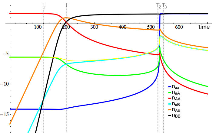
Figure 4. Numerical solution of the deterministic system for $\eta=0.02$, logplot. See Figure 6 for a zoom around the time interval $[T_{2},T_{3}]$.

4. Proof

Definition 4.1.

Let $x,y,z\in\{aa,aA,AA,aB,AB,BB\}$ and $h\in{\mathbb{R}}$. We define

$$T^{x=y} =\inf\{t>0:n_{x}(t)=n_{y}(t)\},$$ (4.1)

$$T^{x=\delta y} =\inf\{t>0:n_{x}(t)=\delta n_{y}(t)\},$$ (4.2)

$$T_{h}^{x} =\inf\{t>0:n_{x}(t)>h\},$$ (4.3)

$$T_{h}^{x+y} =\inf\{t>0:n_{x}(t)+n_{y}(t)>h\},$$ (4.4)

$$T_{h}^{x+y+z} =\inf\{t>0:n_{x}(t)+n_{y}(t)+n_{z}(t)>h\}.$$ (4.5)

Moreover, let

$${\Delta}>\delta>{\varepsilon}_{0}>{\varepsilon}>0.$$ (4.6)

The value ${\varepsilon}_{0}$ is the small order 1 level in the Phase 1, see the proof heuristics (Section 3.2). We consider $\Delta$ fixed and sufficiently small, and will first send ${\varepsilon}\to 0$ and then ${\varepsilon}_{0}\to 0$. A summary of the proof structure can be found in the Appendix A together with the implications between intermediary results.

4.1. Preliminaries

We first state an elementary fact that will be useful throughout the following analysis.

Lemma 4.2.

Let $T>0$ and $f:[0,T]\to{\mathbb{R}}$ be a differentiable function such that $f(0)\leq 0$. If, for all $t\in[0,T]$, $\left\{f(t)=0\Rightarrow\dot{f}(t)<0\right\}$ then $f(t)<0$, for all $t\in(0,T]$.

In the sequel, a part of our majorations and comparison results will rely on this lemma, which ensures that the trajectories of two dynamical systems do not cross as long as the derivative of the upper trajectory is larger than the derivative of the lower one, where these trajectories meet. We will often encounter the situation where $c,T>0$ and $n,g:[0,T]\to{\mathbb{R}}$ are two differentiable functions such that $cn(0)\leq g(0)$.

Then, Lemma 4.2 implies that if, for all $t\in[0,T]$, $\left\{cn(t)=g(t)\Rightarrow c\dot{n}(t)<\dot{g}(t)\right\}$ then $cn(t)\leq g(t)$, for all $t\in[0,T]$.

Proposition 4.3.

We have the following ordering relations:

1. If $n_{AA}(0)\leq\bar{n}_{A}$ then $n_{AA}(t)\leq\bar{n}_{A}$, for all $t>0$.

2. If $n_{BB}(0)<\bar{n}_{B}$ then $n_{BB}(t)\leq\bar{n}_{B}$, for all $t>0$.

3. If $n_{aB}(0)<n_{AB}(0)$ then $n_{aB}(t)\leq n_{AB}(t)$, for all $t>0$.

Proof.

1. We use Lemma 4.2 and show that $\dot{n}_{AA}<0$ at $n_{AA}=\bar{n}_{A}$. For this we construct a majorising process on $n_{AA}$ by comparing the birth and the death rates. Since $\Sigma_{6}\geq\Sigma_{5}$ we get:

   $$b_{AA} \leq{\textstyle{f\over\Sigma_{5}}}n_{AA}(n_{aA}+n_{AA}+n_{AB})+{\textstyle{f\over 4\Sigma_{5}}}\left(n_{aA}^{2}+n_{AB}^{2}\right)$$

   $$\leq fn_{AA}+{\textstyle{f\over 4\Sigma_{5}}}\left(n_{aA}^{2}+n_{AB}^{2}\right),$$ (4.7)

   $$d_{AA} =n_{AA}(D+c\Sigma_{6}),$$ (4.8)

   $$\dot{n}_{AA} \leq n_{AA}(f-D-c\Sigma_{6})+{\textstyle{f\over 4\Sigma_{5}}}\left(n_{aA}^{2}+n_{AB}^{2}\right).$$ (4.9)

   At $n_{AA}=\bar{n}_{A}$ we have

   $$\dot{n}_{AA} \leq n_{aA}\left({\textstyle{f\over 4\Sigma_{5}}}n_{aA}-c\bar{n}_{A}\right)+n_{AB}\left({\textstyle{f\over 4\Sigma_{5}}}n_{AB}-c\bar{n}_{A}\right)$$

   $$\leq n_{aA}\left({\textstyle{f\over 4\Sigma_{5}}}n_{aA}-f+D\right)+n_{AB}\left({\textstyle{f\over 4\Sigma_{5}}}n_{AB}-f+D\right)<0,$$ (4.10)

   since ${\textstyle{f\over 4\Sigma_{5}}}n_{aA}$ and ${\textstyle{f\over 4\Sigma_{5}}}n_{AB}$ are smaller than ${\textstyle{f\over 4}}$.

2. We proceed similarly using Lemma 4.2. We show that $\dot{n}_{BB}<0$ at $n_{BB}=\bar{n}_{B}$ by constructing a majorising process on $n_{BB}$:

   $$b_{BB} ={\textstyle{f\over\Sigma_{5}}}n_{BB}(n_{aB}+n_{AB}+n_{BB})+{\textstyle{f\over 4\Sigma_{5}}}\left(n_{aB}^{2}+n_{AB}^{2}\right)$$

   $$\leq fn_{BB}+{\textstyle{f\over 4\Sigma_{5}}}\left(n_{aB}^{2}+n_{AB}^{2}\right),$$ (4.11)

   $$d_{BB} =n_{BB}(D-{\Delta}+c\Sigma_{5}-\eta n_{aA}),$$ (4.12)

   $$\dot{n}_{BB} \leq n_{BB}(f-D+{\Delta}-c\Sigma_{5}+\eta n_{aA})+{\textstyle{f\over 4\Sigma_{5}}}\left(n_{aB}^{2}+n_{AB}^{2}\right).$$ (4.13)

   At $n_{BB}=\bar{n}_{B}$ we have

   $$\hskip 56.9055pt\dot{n}_{BB} \leq n_{aB}\left({\textstyle{f\over 4\Sigma_{5}}}n_{aB}-c\bar{n}_{B}\right)+n_{AB}\left({\textstyle{f\over 4\Sigma_{5}}}n_{AB}-c\bar{n}_{B}\right)-\bar{n}_{B}(c-\eta)n_{aA}$$

   $$\leq n_{aB}\left({\textstyle{f\over 4\Sigma_{5}}}n_{aB}-f+D-{\Delta}\right)+n_{AB}\left({\textstyle{f\over 4\Sigma_{5}}}n_{AB}-f+D-{\Delta}\right)-\bar{n}_{B}(c-\eta)n_{aA}$$

   $$<0,$$ (4.14)

   since ${\textstyle{f\over 4\Sigma_{5}}}n_{aB}$ and ${\textstyle{f\over 4\Sigma_{5}}}n_{AB}$ are smaller than ${\textstyle{f\over 4}}$ and $\eta\leq c$.

3. Intuitively, this inequality comes from the fact that phenotype $a$ individuals cannot reproduce with phenotype $B$. Indeed, if we consider the couples that could give rise to an $AB$ (resp. $aB$) individual, they are of the form $(Ag_{1},Bg_{2})$ (resp. $(ag_{1},Bg_{2})$), with $g_{1},g_{2}\in\{a,A,B\}$ and the combination $(AA,Bg_{2})$ is possible, whereas $(aa,Bg_{2})$ is impossible. Here is the rigorous derivation of the result: We compare the birth- and the death-rates of $n_{AB}$ and $n_{aB}$, introduced in (2.17),(2.23), and (2.16),(2.22) respectively:

   $$\frac{d_{aB}}{n_{aB}} =D-{\Delta}+c\Sigma_{5}=\frac{d_{AB}}{n_{AB}},$$ (4.15)

   $$b_{aB} =fn_{aB}\frac{{\textstyle{1\over 2}}n_{aB}+{\textstyle{1\over 2}}n_{AB}+n_{BB}}{\Sigma_{5}}+I_{aB},$$ (4.16)

   $$b_{AB} =fn_{AB}\frac{{\textstyle{1\over 2}}n_{aB}+{\textstyle{1\over 2}}n_{AB}+n_{BB}}{\Sigma_{5}}+I_{AB}.$$ (4.17)

   We see that the death-rates of the two populations are the same, whereas the birth-rates differ only in a factor which comes from the reproduction of the other populations. If we take a closer look to these factors $I_{aB},I_{AB}$ under the assumption that $n_{aB}=n_{AB}$ we see that

   $$I_{AB} =f\left({\textstyle{1\over 2}}n_{aA}+n_{AA}\right)\left(\frac{{\textstyle{1\over 2}}n_{aB}+{\textstyle{1\over 2}}n_{AB}+n_{BB}}{\Sigma_{5}}+\frac{{\textstyle{1\over 2}}n_{aB}+{\textstyle{1\over 2}}n_{AB}+n_{BB}}{\Sigma_{6}}\right)$$

   $$=I_{aB}+fn_{AA}\left(\frac{{\textstyle{1\over 2}}n_{aB}+{\textstyle{1\over 2}}n_{AB}+n_{BB}}{\Sigma_{5}}+\frac{{\textstyle{1\over 2}}n_{aB}+{\textstyle{1\over 2}}n_{AB}+n_{BB}}{\Sigma_{6}}\right).$$ (4.18)

   Thus $I_{AB}>I_{aB}$. Hence, $\dot{n}_{AB}>\dot{n}_{aB}$ and $n_{AB}(t)$ stays above $n_{aB}(t)$ for all $t>0$.

∎

4.2. Phase 1: Perturbation of the 3-system $(aa,aA,AA)$ until $AB$ reaches ${\Theta}(1)$

We start with initial conditions given by (2.28)-(2.33). We will show that the mutant population, consisting of all individuals of phenotype $B$, grows up to some ${\varepsilon}_{0}>{\varepsilon}$ without perturbing the behaviour of the 3-system $(aa,aA,AA)$ in this time. Let

$$T_{1}:=T_{{\varepsilon}_{0}}^{{aa+aA+}aB+AB+BB}$$ (4.19)

Proposition 4.4.

With the initial conditions (2.28)-(2.33),

$$T_{1}=T_{{\varepsilon}_{0}}^{AB}={\Theta}\left(\log(({{\varepsilon}_{0}}/{{\varepsilon}^{3}})^{\frac{1}{\Delta-{\Theta}({\varepsilon}_{0})}}\right).$$ (4.20)

Proof.

Until $T_{1}$ the perturbation of the dynamics of the 3-system $(aa,aA,AA)$ is at most of order ${\varepsilon}_{0}$, by continuity of the solutions of an ODE with respect to initial conditions. We thus have $\bar{n}_{A}-{\Theta}({\varepsilon}_{0})\leq n_{AA}(t)\leq\bar{n}_{A}+{\Theta}({\varepsilon}_{0})$, as well as $n_{aa},n_{aA}\leq{\Theta}({\varepsilon}_{0})$. With this rough bounds we will find finer bounds. Heuristically, the newborns of genotype $aA$ are still in majority produced by recombination of $AA$ and $aA$, because the mutant population is not large enough to contribute. The newborns of genotype $aB$ are in majority produced by reproduction of the $aA$ population with the $B$ population. Finally, the newborns of genotype $aa$ are in majority produced by recombination of $aA$ and $aA$, because the only mutant population which could perturb their dynamics is $aB$, which is of smaller order.

1. We show that $n_{BB}\leq n_{AB}^{2}$. Indeed, we use Lemma 4.2, note that $0=n_{BB}(0)\leq n_{AB}(0)^{2}$, and prove that when $n_{BB}=n_{AB}^{2}$ we have

   $$\frac{d}{dt}(n_{BB}-n_{AB}^{2})=\dot{n}_{BB}-2\dot{n}_{AB}n_{AB}=b_{BB}-2n_{AB}b_{AB}-d_{BB}+2n_{AB}d_{AB}<0.$$ (4.21)

   Indeed, using Proposition 4.3 we can bound (4.21) by

   $${\textstyle{f\over\Sigma_{5}}}(n_{AB}+n_{BB})^{2}-{\textstyle{2f\over\Sigma_{6}}}n_{AB}^{2}n_{AA}-n_{BB}(D-{\Delta}+cn_{AA})+2n_{AB}^{2}(D-{\Delta}+cn_{AA}+{\Theta}({\varepsilon}_{0}))$$

   $$\leq n_{AB}^{2}\left({\textstyle{f\over\bar{n}_{A}}}-f-{\Delta}+{\Theta}({\varepsilon}_{0})\right)<0.$$ (4.22)

   Thus $T_{1}=T_{{\varepsilon}_{0}}^{aa+aA+aB+AB}$.

2. We show that $n_{aB}\leq n_{aA}n_{AB}$. Indeed, we use Lemma 4.2, note that $0=n_{aB}(0)\leq n_{aA}(0)n_{AB}(0)$, and prove that when $n_{aB}=n_{aA}n_{AB}$ we have

   $$\frac{d}{dt}(n_{aB}-n_{aA}n_{AB})=\dot{n}_{aB}-\dot{n}_{aA}n_{AB}-\dot{n}_{AB}n_{aA}$$ (4.23)

   $$=b_{aB}-n_{AB}b_{aA}-n_{aA}b_{AB}-d_{aB}+n_{AB}d_{aA}+n_{aA}d_{AB}<0.$$ (4.24)

   Indeed, using (1) we can bound (4.23) by

   $${\textstyle{f\over 2\Sigma_{5}}}n_{aA}n_{AB}-{\textstyle{2f\over\Sigma_{6}}}n_{aA}n_{AA}n_{AB}+n_{aA}n_{AB}(D+cn_{AA}+{\Theta}({\varepsilon}_{0}))$$

   $$\leq n_{aA}n_{AB}\left({\textstyle{f\over 2\bar{n}_{A}}}-f+{\Theta}({\varepsilon}_{0})\right)<0.$$ (4.25)

   Thus $T_{1}=T_{{\varepsilon}_{0}}^{aa+aA+AB}$.

3. We show that $n_{aa}\leq n_{aA}^{2}$. Indeed, we use Lemma 4.2, note that $n_{aa}(0)\leq n_{aA}(0)^{2}$, and prove that when $n_{aa}=n_{aA}^{2}$ we have

   $$\frac{d}{dt}(n_{aa}-n_{aA}^{2})=\dot{n}_{aa}-2\dot{n}_{aA}n_{aA}=b_{aa}-2n_{aA}b_{aA}-d_{aa}+2n_{aA}d_{aA}<0.$$ (4.26)

   Indeed, using (1) and (2), we can bound (4.26) by

   $${\textstyle{f\over 4\Sigma_{6}}}n_{aA}^{2}-{\textstyle{2f\over S_{6}}}n_{aA}^{2}n_{AA}-n_{aA}^{2}(D+{\Delta}+cn_{AA})+2n_{aA}^{2}(D+cn_{AA}+{\Theta}({\varepsilon}_{0}))$$

   $$\leq n_{aA}^{2}\left({\textstyle{f\over 4\bar{n}_{A}}}-f-{\Delta}+{\Theta}({\varepsilon}_{0})\right)<0.$$ (4.27)

   Thus $T_{1}=T_{{\varepsilon}_{0}}^{aA+AB}$.

4. Now, we show that $T_{1}=T_{{\varepsilon}_{0}}^{AB}$. First, we estimate the maximal time $n_{AB}$ would need to reach the level ${\varepsilon}_{0}$. For this upper bound on the time $T_{{\varepsilon}_{0}}^{AB}$, we have to construct a minorising process for $n_{AB}$. Indeed, let us compare the birth and death rates using the results (1)-(3):

   $$b_{AB} \geq{\textstyle{1\over 2}}n_{AB}\frac{2fn_{AA}}{n_{AA}+{\Theta}({\varepsilon}_{0})}=n_{AB}(f-{\Theta}({\varepsilon}_{0})),$$ (4.28)

   $$d_{AB} \leq n_{AB}(D-{\Delta}+c\bar{n}_{A}+{\Theta}({\varepsilon}_{0}))=n_{AB}(f-{\Delta}+{\Theta}({\varepsilon}_{0})).$$ (4.29)

   Hence, we get for the minorising process

   $$\dot{n}_{AB} \geq n_{AB}({\Delta}-{\Theta}({\varepsilon}_{0})),$$ (4.30)

   $$n_{AB}(t) \geq{\varepsilon}^{3}e^{({\Delta}-{\Theta}({\varepsilon}_{0}))t},$$ (4.31)

   and the time $T_{{\varepsilon}_{0}}^{AB}$ is at most of order ${\Theta}\left(\log(({{\varepsilon}_{0}}/{{\varepsilon}^{3}})^{\frac{1}{\Delta-{\Theta}({\varepsilon}_{0})}}\right)$.
   In a second step we show that $n_{aA}(t)\leq{\varepsilon}e^{{\Theta}({\varepsilon}_{0})t}$ and that the minimal time $n_{aA}$ would need to reach ${\varepsilon}_{0}$ would be bigger than ${\Theta}\left(\log(({{\varepsilon}_{0}}/{{\varepsilon}^{3}})^{\frac{1}{\Delta-{\Theta}({\varepsilon}_{0})}}\right)$. For this we construct a majorising process on $n_{aA}$. The birth rate and the death rate can be bounded by using (1)-(3):

   $$b_{aA} \leq{\textstyle{f\over\Sigma_{6}}}n_{AA}n_{aA}+n_{aA}{\Theta}({\varepsilon}_{0}),$$ (4.32)

   $$d_{aA} \geq n_{aA}(f-{\Theta}({\varepsilon}_{0})),$$ (4.33)

   and we get that

   $$\dot{n}_{aA} \leq{\Theta}({\varepsilon}_{0})n_{aA},$$ (4.34)

   $$n_{aA}(t) \leq{\varepsilon}e^{{\Theta}({\varepsilon}_{0})t}.$$ (4.35)

   Thus the minimal time $n_{aA}$ would need to reach ${\varepsilon}_{0}$ is ${\Theta}\left(\log({\varepsilon}_{0}/{\varepsilon})^{{\textstyle{1\over{\Theta}({\varepsilon}_{0})}}}\right)$ which is bigger than the maximal time $n_{AB}$ would need to reach the level ${\varepsilon}_{0}$. Thus $T_{1}=T_{{\varepsilon}_{0}}^{AB}$.

5. It is left to show that $T_{1}\geq{\Theta}\left(\log(({{\varepsilon}_{0}}/{{\varepsilon}^{3}})^{\frac{1}{\Delta-{\Theta}({\varepsilon}_{0})}}\right)$. For this lower bound on the time $T_{1}$, we have to construct a majorising process for $n_{AB}$:

   $$b_{AB} \leq{\textstyle{f\over\Sigma_{5}}}n_{AB}(n_{aA}+n_{AA}+n_{AB})+{\textstyle{f\over\Sigma_{5}}}(n_{aB}+2n_{BB})(n_{aA}+n_{AA}+n_{AB})$$

   $$\leq fn_{AB}+f(n_{aB}+2n_{BB})$$ (4.36)

   Using (1),(2) and (4) we can further bound this by:

   $$b_{AB} \leq fn_{AB}+f(n_{aA}n_{AB}+2n_{AB}^{2})$$

   $$\leq n_{AB}(f+{\Theta}({\varepsilon}_{0})),$$ (4.37)

   $$d_{AB} \geq n_{AB}(D-{\Delta}+c\bar{n}_{A}-{\Theta}({\varepsilon}_{0}))=n_{AB}(f-{\Delta}-{\Theta}({\varepsilon}_{0})).$$ (4.38)

   Hence, we get for the majorising process

   $$\dot{n}_{AB}\leq n_{AB}({\Delta}+{\Theta}({\varepsilon}_{0})),$$ (4.39)

   $$n_{AB}(t)\leq{\varepsilon}^{3}e^{({\Delta}+{\Theta}({\varepsilon}_{0}))t},$$ (4.40)

   and the time $T_{1}$ is at least of order ${\Theta}\left(\log(({{\varepsilon}_{0}}/{{\varepsilon}^{3}})^{\frac{1}{\Delta-{\Theta}({\varepsilon}_{0})}}\right)$.

∎

Corollary 4.5.

With the initial conditions (2.28)-(2.33), for all $t\in[0,T_{1}]$, the following statements hold:

1. $n_{AB}$ grows exponentially with rate ${\Delta}$. It reaches the level ${\varepsilon}_{0}$ in a time at most of order ${\Theta}\left(\log\left(({{\varepsilon}_{0}}/{{\varepsilon}^{3}})^{\frac{1}{\Delta-{\Theta}({\varepsilon}_{0})}}\right)\right)$.

2. $n_{BB}\leq n_{AB}^{2}$,

3. $n_{aB}\leq{\Theta}({\varepsilon}^{1-{\Theta}({\varepsilon}_{0})}{\varepsilon}_{0})$, $n_{aA}\leq{\Theta}({\varepsilon}^{1-{\Theta}({\varepsilon}_{0})})$, $n_{aa}\leq{\Theta}({\varepsilon}^{2-{\Theta}({\varepsilon}_{0})})$ and
   $\bar{n}_{A}-{\Theta}({\varepsilon}_{0})\leq n_{AA}\leq\bar{n}_{A}+{\Theta}({\varepsilon}_{0})$.

Proof.

1. is a direct consequence of Proposition 4.4, see proof of points (4) and (5).

2. is a direct consequence of Proposition 4.4, see proof of points (1).

3. follows from the proof of Proposition 4.4 together with $\bar{n}_{A}-{\Theta}({\varepsilon})\leq\Sigma_{5}\leq\bar{n}_{A}+2{\Delta}{\varepsilon}_{0}$, which we prove now.
   Using the results of Proposition 4.4 we construct a minorising and a majorising processes on $\Sigma_{5}$:

   $$b_{\Sigma_{5}} \leq f\Sigma_{5}+{\Theta}(n_{aa}),$$ (4.41)

   $$b_{\Sigma_{5}} \geq f\Sigma_{5}-{\Theta}(n_{aA}^{2}),$$ (4.42)

   $$d_{\Sigma_{5}} \geq\Sigma_{5}(D+c\Sigma_{5})-({\Delta}+2\eta n_{aA})(n_{aB}+n_{AB}+n_{BB}),$$ (4.43)

   $$d_{\Sigma_{5}} \leq\Sigma_{5}(D+c\Sigma_{5}+cn_{aa}),$$ (4.44)

   $$\dot{\Sigma}_{5} \leq\Sigma_{5}(f-D-c\Sigma_{5})+({\Delta}+2\eta n_{aA})(n_{aB}+n_{AB}+n_{BB}),$$ (4.45)

   $$\dot{\Sigma}_{5} \geq\Sigma_{5}(f-D-c\Sigma_{5}-cn_{aa}).$$ (4.46)

   We use Lemma 4.2: at time 0 the bounds are fulfilled; moreover, at the upper bound we have $\dot{\Sigma}_{5}<0$ and at the lower bound $\dot{\Sigma}_{5}>0$, which ensures the claimed bounds.

∎

Note that Corollary 4.5 implies that

$$T_{1}=T_{{\varepsilon}_{0}}^{aB+AB+BB}=T_{{\varepsilon}_{0}}^{AB}={\Theta}\left(\log\left(\left({{\varepsilon}_{0}}/{{\varepsilon}^{3}}\right)^{\frac{1}{\Delta-{\Theta}({\varepsilon}_{0})}}\right)\right).$$ (4.47)

4.3. Phase 2: Perturbation of the 3-system $(AA,AB,BB)$ until $n_{aA}={\Theta}(n_{AA})$

The initial conditions at the beginning of the second phase are:

$$n_{aa}(T_{1})\leq{\Theta}\left({\varepsilon}^{2-{\Theta}({\varepsilon}_{0})}\right)$$ (4.48)

$$n_{aA}(T_{1})\leq{\Theta}\left({\varepsilon}^{1-{\Theta}({\varepsilon}_{0})}\right)$$ (4.49)

$$\bar{n}_{A}-{\Theta}({\varepsilon}_{0})\leq n_{AA}(T_{1})\leq\bar{n}_{A}$$ (4.50)

$$n_{aB}(T_{1})\leq{\Theta}\left({\varepsilon}^{1-{\Theta}({\varepsilon}_{0})}{\varepsilon}_{0}\right)$$ (4.51)

$$n_{AB}(T_{1})={\varepsilon}_{0}$$ (4.52)

$$n_{BB}(T_{1})\leq{\Theta}\left({\varepsilon}_{0}^{2}\right)$$ (4.53)

Let $\delta>0$ (to be chosen sufficiently small in the sequel). Let

$$T_{2}:=T^{aA=\delta AA}\land T^{aB=\delta AB}\land T^{aa=aA\wedge aB}.$$ (4.54)

As the process stays uniformly bounded in time, observe that until $T_{2}$ we automatically have

$$n_{aa},n_{aA},n_{aB}\leq{\Theta}(\delta).$$ (4.55)

We will show that for $t\in[T_{1},T_{2}]$ the system behaves as a main 3-system $(AA,AB,BB)$ plus perturbations of order $\delta$. The 3-system $(AA,AB,BB)$ behaves exactly the same as in [27] since the parameters satisfy the same hypotheses (slightly lower death rate for phenotype $B$ than for phenotype $A$ individuals, and constant competition parameters).

Moreover, the crucial role of the parameter $\eta$ is that the population containing an allele $a$ only continues to grow in this phase when $\eta$ is large enough. This is due to the smaller competition that $aA$ feels from $BB$, the $aA$ population is thus higher and induces the growth of $aB$.

We start by considering how the growth of $aa,aA$- and $aB$ populations can perturb the 3-system $(AA,AB,BB)$.

Lemma 4.6.

Let $n_{.}^{up}(t)$ be the population of the unperturbed 3- system $(AA,AB,BB)$, that is the solution to (2.25) with $n_{aa}=n_{aA}=n_{aB}=0$. The 3-system $(AA,AB,BB)$ satisfies

$$\dot{n}_{BB} \geq\dot{n}_{BB}^{up}-(n_{aA}+n_{aB})\left({\textstyle{f\left({\textstyle{1\over 2}}n_{AB}+n_{BB}\right)^{2}\over(n_{AA}+n_{AB}+n_{BB})^{2}}}+cn_{BB}\right),$$ (4.56)

$${\dot{n}_{BB}} {\leq\dot{n}_{BB}^{up}+(n_{aA}+n_{aB})\left(\frac{f\left({\textstyle{1\over 4}}n_{aB}+{\textstyle{1\over 2}}n_{AB}+n_{BB}\right)}{\Sigma_{5}}+cn_{BB}\right)},$$ (4.57)

$$\dot{n}_{AB} \geq\dot{n}_{AB}^{up}-(n_{aa}+n_{aA}+n_{aB})\left(\frac{f(n_{AB}+n_{AA})\left({\textstyle{1\over 2}}n_{AB}+n_{BB}\right)}{(n_{AA}+n_{AB}+n_{BB})^{2}}+cn_{AB}\right),$$ (4.58)

$$\dot{n}_{AB} \leq\dot{n}_{AB}^{up}+{\textstyle{f\over\Sigma_{5}}}n_{aA}\left({\textstyle{1\over 2}}n_{aB}+{\textstyle{1\over 2}}n_{AB}+n_{BB}\right)+{\textstyle{f\over\Sigma_{5}}}n_{aB}\left({\textstyle{1\over 2}}n_{AB}+n_{AA}\right),$$ (4.59)

$$\dot{n}_{AA} \geq\dot{n}_{AA}^{up}-(n_{aa}+n_{aA}+n_{aB})\left({\textstyle{f\left({\textstyle{1\over 2}}n_{aA}+{\textstyle{1\over 2}}n_{AB}+n_{AA}\right)^{2}\over(n_{AA}+n_{AB}+n_{BB})2}}+cn_{AA}\right),$$ (4.60)

$$\dot{n}_{AA} \leq\dot{n}_{AA}^{up}+{\textstyle{f\over 2\Sigma_{5}}}n_{aA}\left({\textstyle{1\over 2}}n_{aA}+n_{AB}+n_{AA}\right).$$ (4.61)

Proof.

We consider the rates of $AA,AB$ and $BB$ under the perturbation of $aa,aA$ and $aB$:

$$b_{BB}= \frac{f}{\Sigma_{5}}\left({\textstyle{1\over 2}}n_{AB}+n_{BB}\right)^{2}+\frac{fn_{aB}\left({\textstyle{1\over 4}}n_{aB}+{\textstyle{1\over 2}}n_{AB}+n_{BB}\right)}{\Sigma_{5}}$$

$$= b_{BB}^{up}-\frac{f\left(\left({\textstyle{1\over 2}}n_{AB}+n_{BB}\right)^{2}(n_{aA}+n_{aB})\right)}{\Sigma_{5}(n_{AA}+n_{AB}+n_{BB})}+\frac{fn_{aB}\left({\textstyle{1\over 4}}n_{aB}+{\textstyle{1\over 2}}n_{AB}+n_{BB}\right)}{\Sigma_{5}},$$ (4.62)

$$d_{BB}= d_{BB}^{up}+cn_{BB}(n_{aB}+n_{aA})-\eta n_{aA}n_{BB}.$$ (4.63)

Thus,

$$\dot{n}_{BB}\leq \dot{n}_{BB}^{up}+{\textstyle{f\over\Sigma_{5}}}n_{aB}\left({\textstyle{1\over 4}}n_{aB}+{\textstyle{1\over 2}}n_{AB}+n_{BB}\right)+\eta n_{aA}n_{BB},$$ (4.64)

$$\dot{n}_{BB}\geq \dot{n}_{BB}^{up}-\frac{f(n_{aA}+n_{aB})\left({\textstyle{1\over 2}}n_{AB}+n_{BB}\right)^{2}}{\Sigma_{5}(n_{AA}+n_{AB}+n_{BB})}-cn_{BB}(n_{aA}+n_{aB}).$$ (4.65)

For the $AB$ population we get:

$$b_{AB}= \frac{2f\left({\textstyle{1\over 2}}n_{AB}+n_{BB}\right)\left({\textstyle{1\over 2}}n_{AB}+n_{AA}\right)}{\Sigma_{5}}-\frac{fn_{aa}n_{AA}\left({\textstyle{1\over 2}}n_{aB}+{\textstyle{1\over 2}}n_{AB}+n_{BB}\right)}{\Sigma_{5}\Sigma_{6}}+\frac{f(n_{AA}+n_{AB})}{2\Sigma_{5}}n_{aB}$$

$$+\frac{fn_{aB}n_{AA}}{2\Sigma_{6}}+\frac{fn_{aA}\left({\textstyle{1\over 2}}n_{aB}+{\textstyle{1\over 2}}n_{AB}+n_{BB}\right)}{2\Sigma_{5}}+\frac{fn_{aA}\left({\textstyle{1\over 2}}n_{aB}+{\textstyle{1\over 2}}n_{AB}+n_{BB}\right)}{2\Sigma_{6}}$$

$$= b_{AB}^{up}+n_{aA}\left({\textstyle{1\over 2}}n_{aB}+{\textstyle{1\over 2}}n_{AB}+n_{BB}\right)\left({\textstyle{f\over 2\Sigma_{5}}}+{\textstyle{f\over 2\Sigma_{6}}}\right)+n_{aB}n_{AA}\left({\textstyle{f\over 2\Sigma_{5}}}+{\textstyle{f\over 2\Sigma_{6}}}\right)+\frac{fn_{aB}n_{AB}}{2\Sigma_{5}}$$

$$-\frac{fn_{aa}n_{AA}\left({\textstyle{1\over 2}}n_{aB}+{\textstyle{1\over 2}}n_{AB}+n_{BB}\right)}{\Sigma_{5}\Sigma_{6}}-\frac{2f\left({\textstyle{1\over 2}}n_{AB}+n_{AA}\right)\left({\textstyle{1\over 2}}n_{AB}+n_{BB}\right)(n_{aA}+n_{aB})}{\Sigma_{5}(n_{AA}+n_{AB}+n_{BB})},$$ (4.66)

$$d_{AB}= d_{AB}^{up}+cn_{AB}(n_{aB}+n_{aA}),$$ (4.67)

$$\dot{n}_{AB}\leq \dot{n}_{AB}^{up}+{\textstyle{f\over\Sigma_{5}}}n_{aA}\left({\textstyle{1\over 2}}n_{aB}+{\textstyle{1\over 2}}n_{AB}+n_{BB}\right)+{\textstyle{f\over\Sigma_{5}}}n_{aB}n_{AA}+{\textstyle{f\over 2\Sigma_{5}}}n_{aB}n_{AB},$$ (4.68)

$$\dot{n}_{AB}\geq \dot{n}_{AB}^{up}-{\textstyle{f\left({\textstyle{1\over 2}}n_{aB}+{\textstyle{1\over 2}}n_{AB}+n_{BB}\right)\over\Sigma_{5}\Sigma_{6}}}n_{aa}n_{AA}-{\textstyle{2f\left({\textstyle{1\over 2}}n_{AB}+n_{AA}\right)\left({\textstyle{1\over 2}}n_{AB}+n_{BB}\right)\over\Sigma_{5}(n_{AA}+n_{AB}+n_{BB})}}(n_{aA}+n_{aB})-cn_{AB}(n_{aB}+n_{aA}).$$ (4.69)

And finally for the $AA$ population:

$$b_{AA}= \frac{f\left({\textstyle{1\over 2}}n_{AB}+n_{AA}\right)^{2}}{\Sigma_{5}}+\frac{fn_{aA}n_{AB}}{4\Sigma_{5}}-\frac{fn_{aa}n_{AA}\left({\textstyle{1\over 2}}n_{aA}\!+\!n_{AA}\!+\!{\textstyle{1\over 2}}n_{AB}\right)}{\Sigma_{5}\Sigma_{6}}+\frac{fn_{aA}\left({\textstyle{1\over 2}}n_{aA}\!+\!n_{AA}\!+\!{\textstyle{1\over 2}}n_{AB}\right)}{2\Sigma_{6}}$$

$$= b_{AA}^{up}-\frac{f\left({\textstyle{1\over 2}}n_{AB}+n_{AA}\right)^{2}(n_{aA}+n_{aB})}{\Sigma_{5}(n_{AA}+n_{AB}+n_{BB})}+\frac{fn_{aA}n_{AB}}{4\Sigma_{5}}-\frac{fn_{aa}n_{AA}\left({\textstyle{1\over 2}}n_{aA}+n_{AA}+{\textstyle{1\over 2}}n_{AB}\right)}{\Sigma_{5}\Sigma_{6}}$$

$$+\frac{fn_{aA}\left({\textstyle{1\over 2}}n_{aA}+n_{AA}+{\textstyle{1\over 2}}n_{AB}\right)}{2\Sigma_{6}},$$ (4.70)

$$d_{AA}= d_{AA}^{up}+cn_{AA}(n_{aa}+n_{aA}+n_{aB}),$$ (4.71)

$$\dot{n}_{AA}\leq \dot{n}_{AA}^{up}+\frac{fn_{aA}n_{AB}}{4\Sigma_{5}}+\frac{fn_{aA}\left({\textstyle{1\over 2}}n_{aA}+n_{AA}+{\textstyle{1\over 2}}n_{AB}\right)}{2\Sigma_{6}},$$ (4.72)

$$\dot{n}_{AA}\geq \dot{n}_{AA}^{up}-\frac{f\left({\textstyle{1\over 2}}n_{aA}+{\textstyle{1\over 2}}n_{AB}+n_{AA}\right)^{2}(n_{aa}+n_{aA}+n_{aB})}{\Sigma_{5}(n_{AA}+n_{AB}+n_{BB})}-cn_{AA}(n_{aa}+n_{aA}+n_{aB}).$$ (4.73)

∎

As solutions of a dynamical system are continuous with respect to its parameters (in particular with respect to $\delta$), the latter lemma shows that until $T_{2}$, the 3-system $(AA,AB,BB)$ is at most perturbed by ${\Theta}(\delta)$. We will show that $T_{2}$ diverges with ${\varepsilon}$. Thus, for small enough ${\delta}$, $AB$ will have time to reach the small fixed value $\sqrt{{\varepsilon}_{0}}>0$ in this phase, and we can use the asymptotic decay $1/t$ of the $AB$ and $1/t^{2}$ of the $AA$ populations, which is proved in [27]. We now start to analyse the growth of the small $aa$-, $aA$- and $aB$ populations. The sum-process $\Sigma_{5}$ plays a crucial role for the behaviour of the system in this phase and we need finer bounds on it.

Remark.

In the sequel we often use that $\Sigma_{5}\leq\Sigma_{6}\leq\Sigma_{5}+{\Theta}({\delta})$, which follows from (4.55) and Lemma 4.6.

Proposition 4.7.

The sum-process $\Sigma_{5}=n_{aA}+n_{AA}+n_{aB}+n_{AB}+n_{BB}$ satisfies for all $t\in[T_{1},T_{2}]$:

$$\bar{n}_{B}-\frac{{\Delta}}{c\bar{n}_{B}}n_{AA}-\frac{{\Delta}^{2}}{c\bar{n}_{B}}n_{AA}\leq\Sigma_{5}\leq\bar{n}_{B}-\frac{{\Delta}}{c\bar{n}_{B}}n_{AA}+\frac{{\Delta}^{2}}{c\bar{n}_{B}}n_{AA}.$$ (4.74)

Proof.

We estimate a minorising process and a majorising process on $\Sigma_{5}$:

$$b_{\Sigma_{5}}\leq f(n_{AA}+n_{AB}+n_{BB})$$

$$+f\frac{(n_{aA}+n_{aB})({\textstyle{3\over 4}}n_{aA}+n_{AA}+{\textstyle{3\over 4}}n_{aB}+n_{AB}+n_{BB})}{\Sigma_{5}}+{\Theta}({\delta})\leq f\Sigma_{5}+{\Theta}({\delta}),$$ (4.75)

$$b_{\Sigma_{5}}\geq f(n_{AA}+n_{AB}+n_{BB})$$

$$+f\frac{(n_{aA}+n_{aB})({\textstyle{3\over 4}}n_{aA}+n_{AA}+{\textstyle{3\over 4}}n_{aB}+n_{AB}+n_{BB})}{\Sigma_{5}}-{\Theta}({\delta})\geq f\Sigma_{5}-{\Theta}({\delta}),$$ (4.76)

$$d_{\Sigma_{5}}\leq \Sigma_{5}(D-{\Delta}+c\Sigma_{5})+{\Delta}(n_{AA}+n_{aA})-2\eta n_{aA}n_{BB}+{\Theta}({\delta}),$$ (4.77)

$$d_{\Sigma_{5}}\geq \Sigma_{5}(D-{\Delta}+c\Sigma_{5})+{\Delta}(n_{AA}+n_{aA})-2\eta n_{aA}n_{BB}.$$ (4.78)

We get

$$\dot{\Sigma}_{5} \leq-c\Sigma_{5}^{2}+\Sigma_{5}(f-D+{\Delta})-{\Delta}n_{AA}+{\Theta}(\delta),$$ (4.79)

$$\dot{\Sigma}_{5} \geq-c\Sigma_{5}^{2}+\Sigma_{5}(f-D+{\Delta})-{\Delta}n_{AA}-{\Theta}(\delta).$$ (4.80)

We start with the proof of the upper bound. We use Lemma 4.2 and show that when $\Sigma_{5}$ reaches the upper-bound, it decays faster than the latter. Using (4.79) we compute $\dot{\Sigma}_{5}$ at the bound. Note that if $\Sigma_{5}=\bar{n}_{B}-{\textstyle{{\Delta}\over c\bar{n}_{B}}}n_{AA}+{\textstyle{{\Delta}^{2}\over c\bar{n}_{B}}}n_{AA}$, then $\Sigma_{5}^{2}=\bar{n}_{B}^{2}-{\textstyle{2{\Delta}\over c}}n_{AA}+{\textstyle{{\Delta}^{2}\over c^{2}\bar{n}_{B}^{2}}}n_{AA}^{2}+{\textstyle{2{\Delta}^{2}\over c}}n_{AA}+{\Theta}({\Delta}^{4})n_{AA}^{2}$, thus

$$\dot{\Sigma}_{5}\leq-{\Delta}^{2}n_{AA}-{\textstyle{{\Delta}^{2}\over c\bar{n}_{B}^{2}}}n_{AA}^{2}+{\Theta}({\delta})<0.$$ (4.81)

It is left to show that $\dot{\Sigma}_{5}\leq-{\textstyle{{\Delta}\over c\bar{n}_{B}}}\dot{n}_{AA}+{\textstyle{{\Delta}^{2}\over c\bar{n}_{B}}}\dot{n}_{AA}$. Since we already know (cf. Lemma 4.6) that $(AA,AB,BB)$ behaves like a 3-system with ${\Theta}(\delta)$ perturbations, then $\dot{n}_{AA}\leq 0$, this finishes the proof of the upper bound.

Now we check the lower bound. If $\Sigma_{5}=\bar{n}_{B}-\frac{{\Delta}}{c\bar{n}_{B}}n_{AA}-{\textstyle{{\Delta}^{2}\over c\bar{n}_{B}}}n_{AA}$ then $\Sigma_{5}^{2}=\bar{n}_{B}^{2}-{\textstyle{2{\Delta}\over c}}n_{AA}-{\textstyle{{\Delta}^{2}\over c^{2}\bar{n}_{B}^{2}}}n_{AA}-{\textstyle{2{\Delta}^{2}\over c}}n_{AA}$. Using (4.80), the derivative of $\Sigma_{5}$ at the lower bound is thus bounded by

$$\dot{\Sigma}_{5} \geq{\Delta}^{2}n_{AA}-{\textstyle{{\Delta}^{2}\over c\bar{n}_{B}^{2}}}n_{AA}-{\Theta}\left({\Delta}^{3}\right)n_{AA}^{2}-{\Theta}({\delta})\geq{\Delta}^{2}n_{AA}\left(1-{\textstyle{1+{\Theta}({\Delta})\over c\bar{n}_{B}}}\right)-{\Theta}({\delta})>0.$$ (4.82)

For the second inequality we use that $n_{AA}\leq\bar{n}_{A}$ (Proposition 4.3). By (4.74) and Lemma 4.2, it is enough to show that at the lower bound $\dot{\Sigma}_{5}\geq-{\textstyle{{\Delta}\over c\bar{n}_{B}}}\dot{n}_{AA}$. Since $AA$ is decreasing we have to calculate a majorising process on $AA$:

$$b_{AA} \leq{\textstyle{f\over\Sigma_{5}}}n_{AA}(n_{AA}+n_{AB})+{\textstyle{f\over 4\Sigma_{5}}}n_{AB}^{2}+{\Theta}({\delta}).$$ (4.83)

For the death rate we use that $$\Sigma_{5}\geq\bar{n}_{A}-{\Theta}({\delta})$$:

$$d_{AA} \geq(f-{\Theta}({\delta}))n_{AA},$$ (4.84)

$$\dot{n}_{AA} \leq-{\textstyle{f\over\Sigma_{5}}}n_{AA}n_{BB}+{\textstyle{f\over 4\Sigma_{5}}}n_{AB}^{2}+{\Theta}({\delta}).$$ (4.85)

Hence we have to show that the slope of $\Sigma_{5}$ at the lower bound is bigger than the one of the lower bound, namely we show that ${\Delta}^{2}n_{AA}\left(1-{\textstyle{1+{\Theta}({\Delta})\over c\bar{n}_{B}}}\right)-{\Theta}({\delta})\geq{\textstyle{{\Delta}f\over c\bar{n}_{B}\bar{n}_{A}}}\left(n_{AA}n_{BB}-{\textstyle{1\over 4}}n_{AB}^{2}\right)-{\Theta}({\delta}{\Delta})$, in the case $n_{AA}n_{BB}>{\textstyle{1\over 4}}n_{AB}^{2}$. This is equivalent to show that $\chi:=n_{AA}n_{BB}-{\textstyle{1\over 4}}n_{AB}^{2}\leq{\textstyle{{\Delta}\bar{n}_{A}\over f}}\left(c\bar{n}_{B}-1\right)n_{AA}$. For this we use once again Lemma 4.2 and estimate the derivative of $\chi$ from above with the help of minorising processes on $AA$ and $BB$ and a majorising process on $AB$. For bounding the death rates we use Proposition 4.3:

$$b_{AA} \geq{\textstyle{f\over\Sigma_{5}}}n_{AA}(n_{AA}+n_{AB})+{\textstyle{f\over 4\Sigma_{5}}}n_{AB}^{2}-{\Theta}({\delta}),$$ (4.86)

$$d_{AA} \leq(f+{\Delta})n_{AA}+{\Theta}({\delta}),$$ (4.87)

$$\dot{n}_{AA} \geq-{\textstyle{f\over\Sigma_{5}}}n_{AA}n_{BB}-{\Delta}n_{AA}+{\textstyle{f\over 4\Sigma_{5}}}n_{AB}^{2}-{\Theta}({\delta}).$$ (4.88)

$$b_{BB} \geq{\textstyle{f\over\Sigma_{5}}}n_{BB}(n_{AB}+n_{BB})+{\textstyle{f\over 4\Sigma_{5}}}n_{AB}^{2}-{\Theta}({\delta}),$$ (4.89)

$$d_{BB} \leq fn_{BB},$$ (4.90)

$$\dot{n}_{BB} \geq-{\textstyle{f\over\Sigma_{5}}}n_{AA}n_{BB}+{\textstyle{f\over 4\Sigma_{5}}}n_{AB}^{2}+{\Theta}({\delta}).$$ (4.91)

$$b_{AB} \leq{\textstyle{f\over\Sigma_{5}}}n_{AB}\left(n_{AA}+{\textstyle{1\over 2}}n_{AB}+n_{BB}\right)+{\textstyle{2f\over\Sigma_{5}}}n_{AA}n_{BB}+{\Theta}({\delta}),$$ (4.92)

$$d_{AB} \geq(f-{\Delta})n_{AB},$$ (4.93)

$$\dot{n}_{AB} \leq{\textstyle{2f\over\Sigma_{5}}}n_{AA}n_{BB}-{\textstyle{f\over 2\Sigma_{5}}}n_{AB}^{2}+{\Delta}n_{AB}+{\Theta}({\delta}).$$ (4.94)

The derivative is given by:

$$\dot{\chi} =\dot{n}_{AA}n_{BB}+n_{AA}\dot{n}_{BB}-{\textstyle{1\over 2}}\dot{n}_{AB}n_{AB}$$

$$\leq-f\chi+{\Theta}({\delta}).$$ (4.95)

At the upper bound we get:

$$\dot{\chi}\leq-{\Delta}\bar{n}_{A}(c\bar{n}_{B}-1)n_{AA}+{\Theta}({\delta})<0.$$ (4.96)

It is left to show that at the upper bound $\dot{\chi}\leq{\textstyle{{\Delta}\bar{n}_{A}\over f}}(c\bar{n}_{B}-1)\dot{n}_{AA}$. Using the minorising process $\dot{n}_{AA}\geq-{\Delta}n_{AA}-{\textstyle{f\over\bar{n}_{A}}}\chi-{\Theta}({\delta})$ (see (4.88)), (4.3) and Proposition 4.3 we show that

$${\textstyle{{\Delta}\bar{n}_{A}\over f}}(c\bar{n}_{B}-1)\dot{n}_{AA}+f\chi-{\Theta}({\delta})\geq\chi\left(f-{\Delta}(c\bar{n}_{B}-1)\right)-{\textstyle{{\Delta}^{2}\bar{n}_{A}\over f}}(c\bar{n}_{B}-1)n_{AA}-{\Theta}({\delta})>0.$$ (4.97)

This finishes the proof of the lower bound. ∎

Lemma 4.8.

For $t\in[T_{1},T_{2}]$ and for ${\Delta}$ sufficiently small,

$$\dot{\Sigma}_{aA,aB}\geq-{\Theta}({\Delta})\Sigma_{aA,aB}.$$ (4.98)

Proof.

Using Proposition 4.7, we have the following bound on the process:

$$b_{\Sigma_{aA,aB}} \geq f\frac{n_{aA}({\textstyle{1\over 2}}n_{aA}+n_{AA}+n_{aB}+n_{AB}+n_{BB})+n_{aB}(n_{AA}+{\textstyle{1\over 2}}n_{aB}+n_{AB}+n_{BB})}{n_{aA}+n_{AA}+n_{aB}+n_{AB}+n_{BB}}-{\Theta}({\delta}n_{aA})$$

$$\geq f\Sigma_{aA,aB}-{\Theta}(\delta n_{aA}),$$ (4.99)

$$d_{\Sigma_{aA,aB}} =\Sigma_{aA,aB}(D-{\Delta}+c\Sigma_{5})-\eta n_{aA}n_{BB}+{\Delta}n_{aA}+cn_{aA}n_{aa}$$

$$\leq f\Sigma_{aA,aB}-n_{aA}(\eta n_{BB}-{\Delta})+{\Theta}({\Delta}^{2}n_{AA})\Sigma_{aA,aB}^{2},$$ (4.100)

$$\dot{\Sigma}_{aA,aB} \geq n_{aA}(\eta n_{BB}-{\Delta}-{\Theta}(\delta)){\Theta}({\Delta}^{2}n_{AA})\Sigma_{aA,aB}^{2}\geq n_{aA}(-{\Delta}-{\Theta}(\delta))-{\Theta}({\delta}{\Delta}^{2}n_{AA})\Sigma_{aA,aB}$$

$$\geq\Sigma_{aA,aB}(-{\Delta}-{\Theta}(\delta)).$$ (4.101)

∎

Lemma 4.9.

For all $t\in[T_{1},T_{2}]$ the $aa$ population is bounded by

$$\frac{f}{16\bar{n}_{B}(f+{\Delta}+{\Theta}({\delta}))}\Sigma_{aA,aB}^{2}\leq n_{aa}\leq\frac{f}{\bar{n}_{A}(D+{\Delta})}\Sigma_{aA,aB}^{2}.$$ (4.102)

Observe that this implies $T_{2}=T^{aA=\delta AA}\wedge T^{aB=\delta AB}$.

Proof.

First observe that the inequality is satisfied at $t=T_{1}$. We start with the upper bound and show that $n_{aa}$ would decrease at this bound. For this we estimate a majorising process on $aa$:

$$b_{aa} \leq{\textstyle{f\over\Sigma_{3}}}n_{aa}\left({\textstyle{1\over 2}}n_{aA}+n_{aa}\right)+{\textstyle{f\over 4\Sigma_{5}}}\Sigma_{aA,aB}^{2}+{\textstyle{f\over 2\Sigma_{5}}}n_{aA}n_{aa},$$ (4.103)

$$d_{aa} \geq n_{aa}(D+{\Delta}),$$ (4.104)

$$\dot{n}_{aa} \leq{\textstyle{f\over\Sigma_{3}}}n_{aa}^{2}+{\textstyle{f\over\Sigma_{3}}}n_{aa}n_{aA}+{\textstyle{f\over 4\Sigma_{5}}}\Sigma_{aA,aB}^{2}-n_{aa}(D+{\Delta}).$$ (4.105)

We calculate the slope of this process at the upper bound using Proposition 4.7 and (4.55):

$$\dot{n}_{aa} \leq{\textstyle{f\over 4\Sigma_{5}}}\Sigma_{aA,aB}^{2}-{\textstyle{f\over\bar{n}_{A}}}\Sigma_{aA,aB}^{2}+{\Theta}(\Sigma_{aA,aB}^{2}n_{aA})\leq-{\textstyle{3f-{\Theta}({\delta})\over 4\bar{n}_{A}}}\Sigma_{aA,aB}^{2}<0.$$ (4.106)

By Lemma 4.2, to ensure that (4.102) stays an upper bound it is enough to show that the right-hand side satisfies

$$-{\textstyle{3f-{\Theta}({\delta})\over 4\bar{n}_{A}}}\Sigma_{aA,aB}^{2}\leq{\textstyle{2f\over\bar{n}_{A}(D+{\Delta})}}\dot{\Sigma}_{aA,aB}\Sigma_{aA,aB}.$$ (4.107)

This is a consequence of Lemma 4.8.
For the lower bound we proceed similarly. Since ${\textstyle{1\over\Sigma}}_{6}={\textstyle{1\over\Sigma}}_{5}-{\textstyle{n_{aa}\over\Sigma_{5}\Sigma_{6}}}$ and with the knowledge of the upper bound, we estimate a minorising process on $aa$:

$$b_{aa} \geq{\textstyle{f\over 4\Sigma_{5}}}\Sigma_{aA,aB}^{2}+{\textstyle{f\over 4\Sigma_{6}}}n_{aa}n_{aA}\left(2-{\Theta}({\delta})\right)\geq{\textstyle{f\over 4\Sigma_{5}}}\Sigma_{aA,aB}^{2}.$$ (4.108)

The estimation of the death rate follows from Proposition 4.3 and (4.55)

$$d_{aa} \leq n_{aa}(f+{\Delta}+{\Theta}({\delta})),$$ (4.109)

$$\dot{n}_{aa} \geq{\textstyle{f\over 4\Sigma_{5}}}\Sigma_{aA,aB}^{2}-n_{aa}(f+{\Delta}+{\Theta}({\delta})).$$ (4.110)

With Proposition 4.7 we see that at the lower bound the process increases:

$$\dot{n}_{aa} \geq\left({\textstyle{f\over 4\Sigma_{5}}}-{\textstyle{f\over 16\bar{n}_{B}}}\right)\Sigma_{aA,aB}^{2}>0.$$ (4.111)

By Lemma 4.2, it is left to show that $\dot{n}_{aa}\geq{\textstyle{f\over 8\bar{n}_{B}(f+{\Delta}+{\Theta}({\delta}))}}\dot{\Sigma}_{aA,aB}\Sigma_{aA,aB}$ at the lower bound. Thus we have to calculate a majorising process on $\Sigma_{aA,aB}$:

$$b_{\Sigma_{aA,aB}} \leq f\Sigma_{aA,aB}+{\Theta}\left(\Sigma_{aA,aB}^{2}\right),$$ (4.112)

Using Proposition 4.7, Proposition 4.3 and that $$\eta\leq c$$ we get for the death rate

$$d_{\Sigma_{aA,aB}} \geq(D-{\Delta}+c\Sigma_{5})\Sigma_{aA,aB}+n_{aA}({\Delta}-\eta n_{BB})$$

$$\geq(f-{\Delta}(1+{\Theta}({\Delta})))\Sigma_{aA,aB}-(f-D)\Sigma_{aA,aB}$$

$$=(D-{\Delta}(1+{\Theta}({\Delta})))\Sigma_{aA,aB},$$ (4.113)

$$\dot{\Sigma}_{aA,aB} \leq(f-D+{\Delta}(1+{\Theta}({\Delta})))\Sigma_{aA,aB}+{\Theta}\left(\Sigma_{aA,aB}^{2}\right).$$ (4.114)

Besides we get at the lower bound using Proposition 4.7

$${\textstyle{f(f-D+{\Delta})\over 8\bar{n}_{B}(f+{\Delta}+{\Theta}({\delta}))}}\Sigma_{aA,aB}^{2}-\left({\textstyle{f\over 4\Sigma_{5}}}-{\textstyle{f\over 16\bar{n}_{B}}}\right)\Sigma_{aA,aB}^{2}+{\Theta}(\Sigma_{aA,aB}^{3})$$

$$=-{\textstyle{f\over 16\bar{n}_{B}}}{\textstyle{f+2D+{\Delta}(1-{\Theta}({\Delta}))\over f+{\Delta}+{\Theta}({\delta})}}\Sigma_{aA,aB}^{2}+{\Theta}\left(\Sigma_{aA,aB}^{3}\right)<0.$$ (4.115)

This finishes the proof of the lower bound. ∎

Let

$$T_{=}:=\inf\{t>T_{1}:n_{aA}(t)=n_{aB}(t)\}.$$ (4.116)

Proposition 4.10.

For all $t\in[T_{1},T_{=}]$,

$$n_{aB}\leq n_{aA}={\Theta}({\varepsilon}).$$ (4.117)

Proof.

In this time interval the newborns of genotype $aA$ are in majority produced by reproductions of a population of order one, namely $AB$ or $AA$, with the population $aA$. Since $n_{aA}$ feels competition from a macroscopic population ($AA$, $AB$ or $BB$) the $aA$ population stays of order ${\Theta}({\varepsilon})$. We make this more rigorous. To show this we consider a majorising process on $aA$ and use Proposition 4.7, and Lemma 4.9:

$$b_{aA} \leq fn_{aA}-{\textstyle{f\over\Sigma_{5}}}n_{aA}(n_{BB}+{\textstyle{1\over 2}}n_{AB})+{\textstyle{f\over 2\Sigma_{5}}}n_{aB}(2n_{AA}+n_{AB})+{\Theta}\left(\Sigma_{aA,aB}^{2}\right),$$ (4.118)

$$d_{aA} \geq n_{aA}(f+{\Delta}-{\textstyle{{\Delta}\over\bar{n}_{B}}}n_{AA}-\eta n_{BB}-{\Theta}\left({\Delta}^{2}n_{AA})\right),$$ (4.119)

$$\dot{n}_{aA} \leq-n_{aA}\left(n_{BB}{\textstyle{f-\eta\Sigma_{5}\over\Sigma_{5}}}+{\textstyle{f\over 2\Sigma_{5}}}n_{AB}+{\Delta}\left(1-{\textstyle{n_{AA}\over\bar{n}_{B}}}\right)-{\Theta}\left({\Delta}^{2}n_{AA}\right)\right)+{\textstyle{f\over\Sigma_{5}}}n_{aB}({\textstyle{1\over 2}}n_{AB}+n_{AA}+{\Theta}({\delta}))$$

$$\leq-n_{aA}\left(n_{BB}{\textstyle{D+{\Delta}\over\Sigma_{5}}}+{\textstyle{f\over 2\Sigma_{5}}}n_{AB}+{\Delta}\left(1-{\textstyle{n_{AA}\over\bar{n}_{B}}}\right)-{\Theta}\left({\Delta}^{2}n_{AA}\right)\right)+{\textstyle{f\over\Sigma_{5}}}n_{aB}({\textstyle{1\over 2}}n_{AB}+n_{AA}+{\Theta}({\delta}))$$

$$\leq-n_{aA}\left({\textstyle{f\over\Sigma_{5}}}\left({\textstyle{D+{\Delta}\over f}}n_{BB}+{\textstyle{1\over 2}}n_{AB}\right)+{\Delta}\left(1-{\textstyle{n_{AA}\over\bar{n}_{B}}}\right)-{\Theta}\left({\Delta}^{2}n_{AA}\right)\right)+{\textstyle{f\over\Sigma_{5}}}n_{aB}({\textstyle{1\over 2}}n_{AB}+n_{AA}+{\Theta}({\delta})).$$ (4.120)

By Proposition 4.6 and Proposition 3.4 in [8] there exists a time $t_{0}={\Theta}(1)$ such that the expression in the first bracket becomes bigger than the expression in the second bracket. Thus $n_{aA}$ decreases after $t_{0}$ and since $aA$ does not exceed ${\Theta}({\varepsilon})$ until $t_{0}$ it will stay smaller or equal to ${\Theta}({\varepsilon})$ until $T_{=}$. ∎

We show that as soon as $aB$ crosses $aA$ the $BB$ population is already bigger than or equal to the $AA$ population. First we construct a process that provide an upper bound on $aB$:

Lemma 4.11.

For all $t\in[T_{1},T_{2}]$ the $aB$ population is upper bounded by

$$n_{aB}\leq\frac{n_{AB}+2n_{BB}+{\textstyle{2\Delta\over c}}}{n_{AB}+2n_{AA}}n_{aA}\equiv C(t)n_{aA}.$$ (4.121)

Proof.

First observe that the bound is fulfilled at $t=T_{1}$. Similarly to the proof of Lemma 4.9 we estimate a majorising process on $aB$ given by:

$$\dot{n}_{aB} \leq-n_{aB}\left({\textstyle{f\over 2\Sigma_{5}}}(n_{AB}+2n_{AA})-{\textstyle{\Delta\over\bar{n}_{B}}}n_{AA}-{\Theta}({\Delta}^{2}n_{AA})\right)+n_{aA}{\textstyle{f\over 2\Sigma_{5}}}(n_{AB}+2n_{BB}+{\Theta}({\delta})).$$ (4.122)

By Lemma 4.2, we have to show that as soon as $aB$ reaches the upper bound it decreases faster than the bound, thus we calculate the slope of the majorising process at this value:

$$\dot{n}_{aB} \leq-{\textstyle{f\over 2\Sigma_{5}}}\left(n_{AB}+2n_{BB}+{\textstyle{2{\Delta}\over c}}-{\Theta}({\Delta}^{2}n_{AA})\right)n_{aA}+{\textstyle{{\Delta}\left(n_{AB}+2n_{BB}+2{\Delta}/c\right)\over\bar{n}_{B}(n_{AB}+2n_{AA})}}n_{AA}n_{aA}+{\textstyle{f(n_{AB}+2n_{BB}+{\Theta}({\delta}))\over 2\Sigma_{5}}}n_{aA}$$

Using Proposition 4.7 and that $${\textstyle{n_{AA}\over n_{AB}+2n_{AA}}}\leq{\textstyle{1\over 2}}$$ we get

$$\dot{n}_{aB} \leq-{\textstyle{{\Delta}f-{\Theta}({\Delta}^{2}n_{AA})\over c\Sigma_{5}}}n_{aA}+{\textstyle{{\Delta}\over\Sigma_{5}}}\left({\textstyle{1\over 2}}n_{AB}+n_{BB}+{\textstyle{{\Delta}\over c}}\right)n_{aA}$$

$$\leq{\textstyle{{\Delta}+{\Theta}({\Delta}^{2}n_{AA})+{\Theta}({\delta})\over\Sigma_{5}}}n_{aA}\left(\bar{n}_{B}+{\textstyle{{\Delta}\over c}}-{\textstyle{f\over c}}\right)$$

$$=-{\textstyle{{\Delta}+{\Theta}({\Delta}^{2}n_{AA})+{\Theta}({\delta})\over c\Sigma_{5}}}\left(D-2{\Delta}\right)n_{aA}\leq 0.$$ (4.123)

We have to show that, at the upper bound, $\dot{n}_{aB}<C(t)\dot{n}_{aA}+\dot{C}(t)n_{aA}$. Since the 3-system $(AA,AB,BB)$ converges towards $(0,0,\bar{n}_{B})$, we know from Proposition 3.4 in [8] that $C(t)$ is a monotone increasing function and hence $\dot{C}(t)\geq 0$. Thus if we can show that $\dot{n}_{aB}<C(t)\dot{n}_{aA}$ we are done. For this we have to calculate the slope of the minorising process on $aA$ when $aB$ reaches the upper bound. This process is given by:

$$\dot{n}_{aA} \geq-n_{aA}\left({\textstyle{f\over 2}}+{\Delta}-\eta n_{BB}+{\textstyle{f\over 2\Sigma_{5}}}(n_{BB}-n_{AA})+{\Theta}({\delta})\right)+n_{aB}{\textstyle{f\over 2\Sigma_{5}}}(n_{AB}+2n_{AA}).$$ (4.124)

The slope at the upper bound is:

$$\dot{n}_{aA} \geq-n_{aA}\left({\textstyle{f\over 2}}+{\Delta}-\eta n_{BB}+{\textstyle{f\over 2\Sigma_{5}}}(n_{BB}-n_{AA})-{\textstyle{f\over 2\Sigma_{5}}}\left(n_{AB}+2n_{BB}+{\textstyle{2{\Delta}\over c}}+{\Theta}({\delta})\right)\right)$$

$$\geq-n_{aA}\left({\Delta}-\eta n_{BB}-{\textstyle{{\Delta}f\over c\Sigma_{5}}}+{\Theta}({\delta})\right)$$

$$\geq n_{aA}\left({\Delta}{\textstyle{D-{\Delta}\over c\Sigma_{5}}}+\eta n_{BB}-{\Theta}({\delta})\right)\geq 0.$$ (4.125)

Since $C(t)>0$ this finishes the proof. ∎

Lemma 4.12.

We have $T_{=}<T_{2}$. Moreover,

$$n_{AA}(T_{=})\leq n_{BB}(T_{=})+{\Theta}({\Delta}).$$ (4.126)

Proof.

We first show that $T_{=}<T_{2}$. Using Proposition 4.7 we construct two processes that provide an upper bound and a lower bound on $n_{aB}$. For the birth rates of these processes we use that until time $T_{=}$, $n_{aB}\leq n_{aA}={\Theta}({\varepsilon})$ (Proposition 4.10) and Lemma 4.9:

$$b_{aB} \geq fn_{aB}-{\textstyle{f\over\Sigma_{5}}}n_{aB}({\textstyle{1\over 2}}n_{AB}+n_{AA}+{\Theta}({\varepsilon}))+{\textstyle{f\over\Sigma_{5}}}n_{aA}({\textstyle{1\over 2}}n_{AB}+n_{BB}-{\Theta}({\varepsilon}^{2})),$$ (4.127)

$$b_{aB} \leq fn_{aB}-{\textstyle{f\over\Sigma_{5}}}n_{aB}({\textstyle{1\over 2}}n_{AB}+n_{AA})+{\textstyle{f\over\Sigma_{5}}}n_{aA}({\textstyle{1\over 2}}n_{AB}+n_{BB}+{\Theta}({\varepsilon}^{2})).$$ (4.128)

For the death rates we use Proposition 4.7:

$$d_{aB} \leq n_{aB}f,$$ (4.129)

$$d_{aB} \geq n_{aB}(f-{\textstyle{{\Delta}\over\bar{n}_{B}}}n_{AA}-{\Theta}({\Delta}^{2}n_{AA})),$$ (4.130)

$$\dot{n}_{aB} \leq-n_{aB}\left(\frac{f({\textstyle{1\over 2}}n_{AB}+n_{AA})}{\Sigma_{5}}-{\textstyle{{\Delta}\over\bar{n}_{B}}}n_{AA}-{\Theta}({\Delta}^{2}n_{AA})\right)+n_{aA}\frac{f({\textstyle{1\over 2}}n_{AB}+n_{BB}+{\Theta}({\varepsilon}^{2}))}{\Sigma_{5}},$$ (4.131)

$$\dot{n}_{aB} \geq-n_{aB}\frac{f({\textstyle{1\over 2}}n_{AB}+n_{AA}+{\Theta}({\varepsilon}))}{\Sigma_{5}}+n_{aA}\frac{f({\textstyle{1\over 2}}n_{AB}+n_{BB}-{\Theta}({\varepsilon}^{2}))}{\Sigma_{5}}.$$ (4.132)

We first show that $T_{=}<\infty$. We know that the 3-system $(AA,AB,BB)$ converges to $(0,0,\bar{n}_{B})$ and that $n_{aB}\leq n_{aA}={\Theta}({\varepsilon})$ (Proposition 4.10), for $t\leq T_{=}$. If we assume that $n_{aB}<n_{aA}$, then (4.132) implies that at some time $t_{0}$, where $n_{AB}+2n_{BB}$ is already macroscopic, we have

$$\dot{n}_{aB}\geq{\Theta}({\varepsilon}),\quad n_{aB}\geq{\Theta}({\varepsilon})t.$$ (4.133)

Thus the time $n_{aB}$ needs to reach $n_{aA}={\Theta}({\varepsilon})$ is of order ${\Theta}(1)$. This time is shorter than $T_{aA=\delta AA}$. Indeed, suppose the contrary, then by Proposition 4.10 $n_{aA}$ does not exceed ${\Theta}({\varepsilon})$ before $T_{2}$, and thus $T^{aA=\delta AA}\geq T^{AA}_{{\Theta}({\varepsilon}/\delta)}={\Theta}\left((\delta/{\varepsilon})^{2}\right)$ which diverges with ${\varepsilon}$. A similar reasoning shows that $T_{=}<T^{aB=\delta AB}$. Hence $T_{=}<T_{2}$.
It is left to show that $n_{AA}(T_{=})\leq n_{BB}(T_{=})+{\Theta}({\Delta})$. From Lemma 4.11 we deduce that at $T_{=}$,

$${\textstyle{1\over 2}}n_{AB}+n_{AA} \leq{\textstyle{1\over 2}}n_{AB}+n_{BB}+{\textstyle{{\Delta}\over c}}$$

$$n_{AA} \leq n_{BB}+{\Theta}({\Delta}).$$ (4.134)

∎

Lemma 4.13.

For all $t\in[T_{1},T_{2}]$ the $AB$ population is bounded by

1. $n_{AB}\geq 2\sqrt{\bar{n}_{B}n_{AA}}-2n_{AA}\left(1+{\textstyle{{\Delta}\over c\bar{n}_{B}}}\right)$,

2. $n_{AB}\leq 2\sqrt{\bar{n}_{B}n_{AA}\left(1+{\textstyle{{\Delta}\over f}}\right)}-2n_{AA}$.

Proof.

The proof works like the one of Lemma 4.9. First observe that the bound holds at $t=T_{1}$ which can be proven by using Corollary 4.5 and Proposition 4.7. Then we calculate a minorising process on $AB$:

$$b_{AB} \geq f(2n_{AA}+n_{AB})-{\textstyle{f\over\Sigma_{5}}}(2n_{AA}+n_{AB})(n_{AA}+{\textstyle{1\over 2}}n_{AB}+{\Theta}({\delta})),$$ (4.135)

$$d_{AB} \leq fn_{AB},$$ (4.136)

$$\dot{n}_{AB} \geq-n_{AB}{\textstyle{f\over\Sigma_{5}}}\left({\textstyle{1\over 2}}n_{AB}+n_{AA}+{\Theta}({\delta})\right)+2fn_{AA}-{\textstyle{2f\over\Sigma_{5}}}n_{AA}\left({\textstyle{1\over 2}}n_{AB}+n_{AA}+{\Theta}({\delta})\right).$$ (4.137)

We use Proposition 4.7 and show that this minorising process would increase quicker than the lower bound if $AB$ reaches it:

$$\dot{n}_{AB}\geq -{\textstyle{2f\over\Sigma_{5}}}\left(\sqrt{\bar{n}_{B}n_{AA}}-n_{AA}\left(1+{\textstyle{{\Delta}\over c\bar{n}_{B}}}\right)\right)\left(\sqrt{\bar{n}_{B}n_{AA}}-{\textstyle{{\Delta}\over c\bar{n}_{B}}}n_{AA}+{\Theta}({\delta})\right)$$

$$+2fn_{AA}-{\textstyle{2f\over\Sigma_{5}}}n_{AA}\left(\sqrt{\bar{n}_{B}n_{AA}}-{\textstyle{{\Delta}\over c\bar{n}_{B}}}n_{AA}+{\Theta}({\delta})\right)$$

$$\geq {\textstyle{2f\over\Sigma_{5}}}{\textstyle{{\Delta}\over c\bar{n}_{B}}}n_{AA}\left(2\sqrt{\bar{n}_{B}n_{AA}}-{\textstyle{{\Delta}\over c\bar{n}_{B}}}n_{AA}+{\Theta}({\delta})\right)>0.$$ (4.138)

From Lemma 4.2 it is left to show that at the lower bound,

$$\dot{n}_{AB}\geq\frac{\bar{n}_{B}\dot{n}_{AA}}{\sqrt{\bar{n}_{B}n_{AA}}}-2\dot{n}_{AA}\left(1+{\textstyle{{\Delta}\over c\bar{n}_{B}}}\right).$$ (4.139)

For this we calculate a majorising process on $AA$ using Proposition 4.7 and (4.55):

$$b_{AA} \leq{\textstyle{f\over\Sigma_{5}}}n_{AA}(n_{AA}+n_{AB})+{\textstyle{f\over 4\Sigma_{5}}}n_{AB}^{2}+{\Theta}({\delta}),$$ (4.140)

$$d_{AA} \geq(f-{\Theta}({\Delta}^{2}))n_{AA},$$ (4.141)

$$\dot{n}_{AA} \leq-n_{AA}\left(f-{\textstyle{f\over\Sigma_{5}}}(n_{AA}+n_{AB})-{\Theta}({\Delta}^{2})\right)+{\textstyle{f\over 4\Sigma_{5}}}n_{AB}^{2}+{\Theta}({\delta}).$$ (4.142)

If we now insert the lower bound and use Proposition 4.7 we get,

$$\dot{n}_{AA}\leq-{\textstyle{2f\over\Sigma_{5}}}{\textstyle{{\Delta}\over c\bar{n}_{B}}}n_{AA}\sqrt{\bar{n}_{B}n_{AA}}+{\Theta}({\Delta}^{2})<0.$$ (4.143)

Thus (4.139) is fulfilled.

First, observe that the upper bound is fulfilled at $t=T_{1}$. We then have to estimate a majorising process on $AB$. For the birth rate we use (4.55) and for the death rate we use Proposition 4.7.

$$b_{AB} \leq f(2n_{AA}+n_{AB})-{\textstyle{f\over\Sigma_{5}}}(2n_{AA}+n_{AB})(n_{AA}+{\textstyle{1\over 2}}n_{AB})+{\Theta}({\delta}),$$ (4.144)

$$d_{AB} \geq n_{AB}(D-{\Delta}+c\bar{n}_{B}-{\textstyle{{\Delta}\over\bar{n}_{B}}}n_{AA}-{\Theta}({\Delta}^{2}n_{AA}))$$ (4.145)

$$=n_{AB}(f-{\textstyle{{\Delta}\over\bar{n}_{B}}}n_{AA}-{\Theta}({\Delta}^{2}n_{AA})),$$ (4.146)

$$\dot{n}_{AB} \leq-{\textstyle{f\over 2\bar{n}_{B}}}n_{AB}^{2}-n_{AB}{\textstyle{2f-{\Delta}\over\bar{n}_{B}}}n_{AA}+2fn_{AA}-{\textstyle{2f\over\bar{n}_{B}}}n_{AA}^{2}+{\Theta}({\Delta}^{2}n_{AA}).$$ (4.147)

As before we calculate the slope of this majorising process if it would reach the upper bound:

$$\dot{n}_{AB}\leq-{\textstyle{2{\Delta}\over\bar{n}_{B}}}n_{AA}^{2}+{\Theta}({\Delta}^{2}n_{AA})<0.$$ (4.148)

By Lemma 4.2 we have to show that

$$\dot{n}_{AB}<\dot{n}_{AA}\left({\textstyle{\bar{n}_{B}\left(1+{\Delta}/f\right)\over\sqrt{\bar{n}_{B}n_{AA}\left(1+{\Delta}/f\right)}}}-2\right).$$ (4.149)

For this we calculate the slope of a minorising process on $AA$:

$$b_{AA} \geq{\textstyle{f\over\Sigma_{5}}}n_{AA}(n_{AA}+n_{AB})+{\textstyle{f\over 4\Sigma_{5}}}n_{AB}^{2}-{\Theta}({\delta}^{2}).$$ (4.150)

Using Proposition 4.7 the death rate is bounded by:

$$d_{AA} \leq n_{AA}(f+{\Delta}+{\Theta}({\delta}^{2})),$$ (4.151)

$$\dot{n}_{AA} \geq-n_{AA}\left(f-{\textstyle{f\over\Sigma_{5}}}(n_{AA}+n_{AB})+{\Delta}+{\Theta}({\delta}^{2})\right)+{\textstyle{f\over 4\Sigma_{5}}}n_{AB}^{2}.$$ (4.152)

At the upper bound $AA$ would start to increases:

$$\dot{n}_{AA}\geq{\textstyle{{\Delta}\over\bar{n}_{B}}}n_{AA}^{2}-{\Theta}({\delta}^{2})>0.$$ (4.153)

Thus we get

$$\dot{n}_{AA}\left({\textstyle{\bar{n}_{B}\left(1+{\Delta}/f\right)\over\sqrt{\bar{n}_{B}n_{AA}\left(1+{\Delta}/f\right)}}}-2\right)-\dot{n}_{AB}\geq{\textstyle{{\Delta}\left(1+{\Delta}/f\right)\over\sqrt{\bar{n}_{B}n_{AA}\left(1+{\Delta}/f\right)}}}n_{AA}^{2}-{\Theta}({\Delta}^{2}n_{AA})>0.$$ (4.154)

This finishes the proof of (2). ∎

The following Proposition is a statement for the 3-system $(AA,AB,BB)$ but it remains valid until time $T_{2}$ in the 6-system $(aa,aA,AA,aB,AB,BB)$, for ${\delta}<{\Delta}$.

Proposition 4.14.

The maximal value $n_{AB}^{max}$ of $n_{AB}$ in $[T_{1},T_{2}]$ is bounded by

$$\frac{\bar{n}_{B}}{2}-{\Theta}({\Delta})\leq n_{AB}^{max}\leq\frac{\bar{n}_{B}}{2}+{\Theta}({\Delta}).$$ (4.155)

Moreover, let $T_{AB}^{max}$ be the time when $n_{AB}$ takes its maximum, then $n_{AA}$ and $n_{BB}$ are bounded by

$$\frac{\bar{n}_{B}}{4}-{\Theta}({\Delta})\leq n_{AA}(T_{AB}^{max})\leq\frac{\bar{n}_{B}}{4}+{\Theta}({\Delta}),$$ (4.156)

$$\frac{\bar{n}_{B}}{4}-{\Theta}({\Delta})\leq n_{BB}(T_{AB}^{max})\leq\frac{\bar{n}_{B}}{4}+{\Theta}({\Delta}).$$ (4.157)

Proof.

From Lemma 4.13 (1) we get that

$$n_{AB}\geq 2\sqrt{\bar{n}_{B}n_{AA}}-2n_{AA}\left(1+{\textstyle{{\Delta}\over c\bar{n}_{B}}}\right).$$ (4.158)

We look for the value of $AA$ where the expression on the right hand side takes on its minimum, thus we have to derivate $n_{AA}$ and set it to zero:

$$\frac{\bar{n}_{B}}{\sqrt{\bar{n}_{B}n_{AA}}}-\left(2+{\textstyle{2{\Delta}\over c\bar{n}_{B}}}\right) =0$$ (4.159)

$$\bar{n}_{B}^{2} =\left(4+8{\textstyle{{\Delta}\over c\bar{n}_{B}}}+{\Theta}({\Delta}^{2})\right)\bar{n}_{B}n_{AA}$$ (4.160)

$$\frac{\bar{n}_{B}}{4}-{\Theta}({\Delta}) =n_{AA}.$$ (4.161)

If we insert this in $n_{AB}$ we get the lower bound:

$$n_{AB}\geq{\textstyle{\bar{n}_{B}\over 2}}+{\Theta}({\Delta}).$$ (4.162)

For the upper bound on $n_{AB}$ we proceed similarly. From Lemma 4.13 (2) we get

$$n_{AB}\leq 2\sqrt{\bar{n}_{B}n_{AA}\left(1+{\textstyle{{\Delta}\over f}}\right)}-2n_{AA}.$$ (4.163)

Setting the derivation of the rhs to zero gives:

$$0 ={\textstyle{\bar{n}_{B}\left(1+{\textstyle{{\Delta}\over f}}\right)\over\sqrt{\bar{n}_{B}n_{AA}\left(1+{\textstyle{{\Delta}\over f}}\right)}}}-2$$ (4.164)

$$n_{AA} =\frac{\bar{n}_{B}}{4}+{\Theta}({\Delta}).$$ (4.165)

Finally we get

$$n_{AB}\leq{\textstyle{\bar{n}_{B}\over 2}}-{\Theta}({\Delta})\quad\text{ and }\quad n_{AA}={\textstyle{\bar{n}_{B}\over 4}}-{\Theta}({\Delta}).$$ (4.166)

∎

Remark.

Note that by Proposition 4.7, (4.166) and (4.55) $n_{AA}=n_{BB}\pm{\Theta}({\Delta})={\textstyle{\bar{n}_{B}\over 4}}\pm{\Theta}({\Delta})$ as soon as $n_{AB}$ reaches its maximal value.

Proposition 4.15.

For all $t\in[T_{1},T_{2}]$,

$$n_{aA}\leq{\Theta}({\varepsilon})\vee n_{aB}.$$ (4.167)

Proof.

For $t\leq T_{=}$ this follows from Proposition 4.10. For $t>T_{=}$ we show this by constructing a majorising process of $n_{aA}(t)$. For the birth rate we use (4.55) and Lemma 4.9:

$$b_{aA}\leq f\frac{(n_{aA}+n_{aB})(2n_{AA}+n_{AB}+{\Theta}({\delta}))}{2\Sigma_{5}}$$

$$\leq {\textstyle{f+{\Theta}({\delta})\over 2}}(n_{aA}+n_{aB})+\frac{f(n_{AA}-n_{BB})}{2\bar{n}_{A}}(n_{aA}+n_{aB}).$$ (4.168)

Using Proposition 4.7 and that $${\textstyle{n_{AA}\over\bar{n}_{B}}}<1$$ we get the death rate:

$$d_{aA}\geq n_{aA}\left(D+c\bar{n}_{B}-{\textstyle{{\Delta}\over\bar{n}_{B}}}n_{AA}-\eta n_{BB}-{\Theta}({\Delta}^{2}n_{AA})\right)$$

$$\geq n_{aA}(f-\eta n_{BB}),$$ (4.169)

$$\dot{n}_{aA}\leq -n_{aA}\left({\textstyle{f\over 2}}-{\textstyle{f(n_{AA}-n_{BB})\over 2\bar{n}_{A}}}-\eta n_{BB}-{\Theta}({\delta})\right)+n_{aB}\left({\textstyle{f\over 2}}+{\textstyle{f(n_{AA}-n_{BB}+{\Theta}({\delta}))\over 2\bar{n}_{A}}}\right).$$ (4.170)

By Lemma 4.2, it is left to show that $\dot{n}_{aA}\leq\dot{n}_{aB}$ whenever $n_{aA}=n_{aB}$. At this upper bound we have $\dot{n}_{aA}\leq{n_{aB}}(\frac{f}{\bar{n}_{A}}(n_{AA}-n_{BB})+\eta n_{BB}+{\Theta}({\delta}))$. We now calculate a minorising process on $n_{aB}$. The birth rate can be estimate by using Proposition 4.7, (4.55) and that ${\textstyle{1/2n_{AB}+n_{BB}\over\Sigma_{5}}}\geq{\textstyle{1\over 2}}-{\Theta}({\Delta})$, for $t>T_{=}$:

$$b_{aB} \geq{\textstyle{f\over 2\Sigma_{5}}}(n_{aA}+n_{aB})(n_{aB}+n_{AB}+2n_{BB}).$$ (4.171)

For the death rate Proposition 4.7 is used:

$$d_{aB} \leq n_{aB}(D-\Delta+c\bar{n}_{B})=fn_{aB},$$ (4.172)

$$\dot{n}_{aB} \geq{\textstyle{f\over 2\Sigma_{5}}}n_{aA}(n_{aB}+n_{AB}+2n_{BB})-{\textstyle{f\over 2\Sigma_{5}}}n_{aB}(2n_{AA}+2n_{aA}-n_{aB}-n_{AB}).$$ (4.173)

Thus $\dot{n}_{aB}\geq{\textstyle{f\over\Sigma_{5}}}n_{aB}(n_{BB}-n_{AA}+n_{AB})$ whenever $n_{aA}=n_{aB}$, and hence $\dot{n}_{aB}-\dot{n}_{aA}\geq{\textstyle{f\over\bar{n}_{A}}}n_{aB}(2n_{BB}-2n_{AA}+\eta n_{BB}-{\Theta}(\Delta))>0$ by Proposition 4.14. This finishes the proof. ∎

Now we show that the time $T^{aA=\delta AA}$ is finite and prove that it is smaller than or equal to $T^{aB=\delta BB}$. To estimate the order of magnitude of the time $T_{2}$ we need bounds on $n_{aA}$ which depends on $\Sigma_{aA,aB}$.

Lemma 4.16.

For all $t\in[T_{1},T_{2}]$ the $aA$ population is bounded by

$$\frac{f(n_{AB}+2n_{AA})}{4\bar{n}_{B}(f+\Delta)}\Sigma_{aA,aB}\leq n_{aA}\leq\frac{f(n_{AB}+2n_{AA})}{\bar{n}_{A}(D-2\Delta)}\Sigma_{aA,aB}.$$ (4.174)

Proof.

We start with the upper bound. First observe that it holds at $t=T_{1}$. By Lemma 4.2 it is enough to show that if $n_{aA}$ would reach the upper bound it would decrease faster than the bound. Using Lemma 4.9 and (4.55) the birth rate of a majorising process on $aA$ is given by

$$b_{aA} \leq{\textstyle{f\over 2\Sigma_{5}}}\Sigma_{aA,aB}(n_{AB}+2n_{AA}+{\Theta}({\delta})).$$ (4.175)

For the death rate we use that $$\eta<c,{\textstyle{n_{AA}\over\bar{n}_{B}}}<1$$ and Proposition 4.7:

$$d_{aA} \geq n_{aA}\left(D+c\bar{n}_{B}-{\textstyle{\Delta\over\bar{n}_{B}}}n_{AA}-\eta n_{BB}-{\Theta}({\Delta}^{2}n_{AA})\right)\geq n_{aA}(D-2{\Delta}),$$ (4.176)

$$\dot{n}_{aA} \leq\frac{f(2n_{AA}+n_{AB}+{\Theta}({\delta}))}{2\Sigma_{5}}\Sigma_{aA,aB}-n_{aA}(D-2\Delta).$$ (4.177)

We calculate the slope of the majorising process at the upper bound using Proposition 4.7:

$$\dot{n}_{aA} \leq f(2n_{AA}+n_{AB})\Sigma_{aA,aB}\left({\textstyle{1\over 2\Sigma_{5}}}-{\textstyle{1\over\bar{n}_{A}}}+{\Theta}({\delta})\right)\leq-{\textstyle{f\over 2\bar{n}_{A}}}(2n_{AA}+n_{AB}+{\Theta}({\delta}))\Sigma_{aA,aB}.$$ (4.178)

We have to show that at the upper bound,

$$\dot{n}_{aA}\leq\frac{f(\dot{n}_{AB}+2\dot{n}_{AA})}{\bar{n}_{A}(D-2{\Delta})}\Sigma_{aA,aB}+\frac{f(n_{AB}+2n_{AA})}{\bar{n}_{A}(D-2{\Delta})}\dot{\Sigma}_{aA,aB}.$$ (4.179)

To do this we calculate minorising processes on $n_{AB}$ and $n_{AA}$. For the birth rates we use Lemma 4.9 and (4.55):

$$b_{AB} \geq{\textstyle{f\over\Sigma_{5}}}n_{AB}\left({\textstyle{1\over 2}}n_{aA}+n_{AA}+{\textstyle{1\over 2}}n_{aB}+{\textstyle{1\over 2}}n_{AB}+n_{BB}-{\Theta}({\delta}^{2})\right)+{\textstyle{2f\over\Sigma_{5}}}n_{AA}\left({\textstyle{1\over 2}}n_{aB}+n_{BB}-{\Theta}\left({\delta}^{2}\right)\right),$$ (4.180)

$$b_{AA} \geq{\textstyle{f\over\Sigma_{5}}}n_{AA}\left(n_{aA}+n_{AA}+n_{AB}-{\Theta}\left({\delta}^{2}\right)\right)+{\textstyle{f\over 2\Sigma_{5}}}n_{AB}\left(n_{aA}+{\textstyle{1\over 2}}n_{AB}-{\Theta}\left({\delta}^{2}\right)\right).$$ (4.181)

Applying Proposition 4.7, Lemma 4.9 and (4.55) we get the following death rates:

$$d_{AB} \leq n_{AB}f,$$ (4.182)

$$d_{AA} \leq n_{AA}(f+{\Delta}+{\Theta}({\delta}^{2})).$$ (4.183)

Hence, the minorising processes are given by:

$$\dot{n}_{AB} \geq-{\textstyle{f\over\Sigma_{5}}}n_{AB}\left({\textstyle{1\over 2}}n_{aA}+{\textstyle{1\over 2}}n_{aB}+{\textstyle{1\over 2}}n_{AB}+{\Theta}\left({\delta}^{2}\right)\right)+{\textstyle{2f\over\Sigma_{5}}}n_{AA}\left({\textstyle{1\over 2}}n_{aB}+n_{BB}-{\Theta}\left({\delta}^{2}\right)\right),$$ (4.184)

$$\dot{n}_{AA} \geq-{\textstyle{f\over\Sigma_{5}}}n_{AA}\left(n_{aB}+n_{BB}+{\Theta}\left({\delta}^{2}\right)\right)-{\Delta}n_{AA}+{\textstyle{f\over 2\Sigma_{5}}}n_{AB}\left(n_{aA}+{\textstyle{1\over 2}}n_{AB}-{\Theta}\left({\delta}^{2}\right)\right).$$ (4.185)

From (4.184) and (4.185) we get that

$$\dot{n}_{AB}+2\dot{n}_{AA} \geq{\textstyle{f\over\Sigma_{5}}}n_{AB}\left({\textstyle{1\over 2}}n_{aA}-{\textstyle{1\over 2}}n_{aB}-{\Theta}\left({\delta}^{2}\right)\right)+{\textstyle{2f\over\Sigma_{5}}}n_{AA}\left(-{\textstyle{1\over 2}}n_{aB}-{\Theta}\left({\delta}^{2}\right)\right)-2{\Delta}n_{AA}$$

$$\geq-2{\Delta}n_{AA}-{\Theta}\left({\delta}\right)(n_{AA}+n_{AB}).$$ (4.186)

By Lemma 4.8, we know that $\dot{\Sigma}_{aA,aB}\geq-{\Delta}\Sigma_{aA,aB}$. Thus, using (4.186) the right-hand side minus the left-hand side of (4.179) is bounded from below by

$$-\frac{2{\Delta}n_{AA}f\Sigma_{aA,aB}}{\bar{n}_{A}(D-2{\Delta})}-\frac{{\Delta}(n_{AB}+2n_{AA})\Sigma_{aA,aB}}{\bar{n}_{A}(D-2{\Delta})}+\frac{f\left(2n_{AA}+n_{AB}+{\Theta}\left({\delta}\right)\right)\Sigma_{aA,aB}}{2\bar{n}_{A}}$$

$$\hskip 307.28984pt-{\Theta}\left({\delta}\right)\Sigma_{aA,aB}(n_{AA}+n_{AB})$$

$$\geq\frac{fn_{AA}\Sigma_{aA,aB}}{\bar{n}_{A}}\left(1-\frac{2{\Delta}+{\Theta}({\delta})}{D-2{\Delta}}\right)+\frac{fn_{AB}\Sigma_{aA,aB}}{2\bar{n}_{A}}\left(1-\frac{2{\Delta}+{\Theta}({\delta})}{D-2{\Delta}}\right)>0.$$ (4.187)

This finishes the proof of (1).

For the lower bound we proceed similarly (using Lemma 4.2). This time we show that if $n_{aA}$ would reach the lower bound it would start to increase faster than the bound. Thus we need a minorising process on $n_{aA}$. Using Lemma 4.9 and (4.55) the birth rate of such a process is given by

$$b_{aA} \geq{\textstyle{f\over 2\Sigma_{5}}}\Sigma_{aA,aB}\left(2n_{AA}+n_{AB}-{\Theta}\left({\delta}^{2}\right)\right).$$ (4.188)

With Proposition 4.7 we get:

$$d_{aA} \leq n_{aA}\left(f+\Delta+{\Theta}\left({\delta}^{2}\right)\right),$$ (4.189)

$$\dot{n}_{aA} \geq\frac{f\left(2n_{AA}+n_{AB}-{\Theta}\left({\delta}^{2}\right)\right)}{2\bar{n}_{B}}\Sigma_{aA,aB}-n_{aA}(f+\Delta).$$ (4.190)

We calculate the slope of the minorising process at the lower bound:

$$\dot{n}_{aA} \geq\frac{f\left(2n_{AA}+n_{AB}-{\Theta}\left({\delta}^{2}\right)\right)}{2\bar{n}_{B}}\Sigma_{aA,aB}-\frac{f(2n_{AA}+n_{AB})}{4\bar{n}_{B}}\Sigma_{aA,aB}$$

$$=\frac{f\left(2n_{AA}+n_{AB}-{\Theta}\left({\delta}^{2}\right)\right)}{4\bar{n}_{B}}\Sigma_{aA,aB}>0.$$ (4.191)

Thus the minorising process on $n_{aA}$ would increase when the $aA$ population would reach the lower bound. To ensure this lower bound we have to show

$$\dot{n}_{aA}\geq\frac{f(\dot{n}_{AB}+2\dot{n}_{AA})}{4\bar{n}_{B}(f+{\Delta})}\Sigma_{aA,aB}+\frac{f(n_{AB}+2n_{AA})}{4\bar{n}_{B}(f+{\Delta})}\dot{\Sigma}_{aA,aB}.$$ (4.192)

For this we consider a majorising process on $\Sigma_{aA,aB}$. The birth rate is the same as in (4.112) and the death rate can be lower bounded by using Proposition 4.7 and Lemma 4.9:

$$d_{\Sigma_{aA,aB}} \geq\Sigma_{aA,aB}\left(f-{\textstyle{{\Delta}\over\bar{n}_{B}}}n_{AA}-{\textstyle{{\Delta}^{2}\over\bar{n}_{B}}}n_{AA}\right)+n_{aA}({\Delta}-\eta n_{BB})+{\Theta}\left(\Sigma_{aA,aB}^{3}\right).$$ (4.193)

Hence, we get:

$$\dot{\Sigma}_{aA,aB} \leq{\textstyle{\Delta\over\bar{n}_{B}}}n_{AA}\Sigma_{aA,aB}-n_{aA}(\Delta-\eta n_{BB})+{\Theta}({\Delta}^{2}n_{AA})\Sigma_{aA,aB}.$$ (4.194)

Using that $\eta<c$, the slope of this process if $n_{aA}$ reaches the lower bound is estimated by

$$\dot{\Sigma}_{aA,aB} \leq{\textstyle{\Delta\over\bar{n}_{B}}}n_{AA}\Sigma_{aA,aB}-\frac{f(2n_{AA}+n_{AB})}{4\bar{n}_{B}(f+\Delta)}(\Delta-\eta n_{BB})\Sigma_{aA,aB}+{\Theta}({\Delta}^{2}n_{AA})\Sigma_{aA,aB}$$

$$\leq\frac{f(2n_{AA}+n_{AB})}{4\bar{n}_{B}}\frac{f-D}{f+\Delta}\Sigma_{aA,aB}+{\textstyle{\Delta\over\bar{n}_{B}}}n_{AA}\Sigma_{aA,aB}+{\Theta}({\Delta}^{2}n_{AA})\Sigma_{aA,aB}.$$ (4.195)

Moreover we need majorising processes on $AA$ and $AB$. Using (4.55) the birth rates of these processes can be bounded by:

$$b_{AB} \leq{\textstyle{f\over\Sigma_{5}}}n_{AB}\left({\textstyle{1\over 2}}n_{AB}+n_{AA}+n_{BB}\right)+{\textstyle{2f\over\Sigma_{5}}}n_{AA}n_{BB}+{\Theta}({\delta}),$$ (4.196)

$$b_{AA} \leq{\textstyle{f\over\Sigma_{5}}}n_{AA}\left(n_{AB}+n_{AA}\right)+{\textstyle{f\over 4\Sigma_{5}}}n_{AB}^{2}+{\Theta}({\delta}).$$ (4.197)

For bounding the death rates we apply Proposition 4.7:

$$d_{AB} \geq n_{AB}\left(f-{\textstyle{{\Delta}(1+{\Delta})\over\bar{n}_{B}}}n_{AA}\right),$$ (4.198)

$$d_{AA} \geq n_{AA}\left(f+{\Delta}-{\textstyle{{\Delta}(1+{\Delta})\over\bar{n}_{B}}}n_{AA}\right).$$ (4.199)

Hence we get:

$$\dot{n}_{AB} \leq-{\textstyle{f\over 2\Sigma_{5}}}n_{AB}^{2}+{\textstyle{2f\over\Sigma_{5}}}n_{AA}n_{BB}+{\textstyle{{\Delta}(1+{\Delta})\over\bar{n}_{B}}}n_{AA}n_{AB}+{\Theta}({\delta}),$$ (4.200)

$$\dot{n}_{AA} \leq-n_{AA}\left({\textstyle{f\over\Sigma_{5}}}n_{BB}+{\Delta}-{\textstyle{{\Delta}(1+{\Delta})\over\bar{n}_{B}}}n_{AA}\right)+{\textstyle{f\over 4\Sigma_{5}}}n_{AB}^{2}+{\Theta}({\delta}).$$ (4.201)

From (4.200) and (4.201) we get that

$$\dot{n}_{AB}+2\dot{n}_{AA}\leq-{\Delta}n_{AA}\left(2-{\textstyle{2n_{AA}+n_{AB}\over\bar{n}_{B}}}\right)+{\Theta}\left({\Delta}^{2}n_{AA}\right)+{\Theta}({\delta})<{\Theta}\left({\Delta}^{2}n_{AA}+{\delta}\right).$$ (4.202)

Thus for (4.192) it is enough to show that

$$\dot{n}_{aA} \geq\frac{f(2n_{AA}+n_{AB})}{4\bar{n}_{B}(f+\Delta)}\dot{\Sigma}_{aA,aB}+\left({\Theta}\left({\Delta}^{2}n_{AA}\right)+{\Theta}({\delta})\right)\Sigma_{aA,aB},$$ (4.203)

using (4.195) and (4.191) the lhs minus the rhs of (4.203) is given by

$$\frac{f\left(2n_{AA}+n_{AB}-{\Theta}\left({\delta}^{2}\right)\right)}{4\bar{n}_{B}}\Sigma_{aA,aB}-\frac{f^{2}(n_{AB}+2n_{AA})^{2}}{16\bar{n}_{B}^{2}(f+{\Delta})}\frac{f-D}{f+\Delta}\Sigma_{aA,aB}$$

$$\hskip 133.72786pt-\frac{f(n_{AB}+2n_{AA})}{4\bar{n}_{B}(f+{\Delta})}\frac{\Delta}{\bar{n}_{B}}n_{AA}\Sigma_{aA,aB}-{\Theta}\left({\Delta}^{2}n_{AA}+{\delta}\right)\Sigma_{aA,aB}$$

$$\geq\frac{f\left(2n_{AA}+n_{AB}-{\Theta}\left({\delta}^{2}\right)\right)}{4\bar{n}_{B}}\Sigma_{aA,aB}-\frac{f(2n_{AA}+n_{AB})}{8\bar{n}_{B}}\Sigma_{aA,aB}\left(1+\frac{2{\Delta}(1+{\Delta})n_{AA}}{\bar{n}_{B}(f+{\Delta})}\right)-$$

$$\hskip 133.72786pt-{\Theta}\left({\Delta}^{2}n_{AA}+{\delta}\right)\Sigma_{aA,aB}>0.$$ (4.204)

For the first inequality we use the rough estimations ${\textstyle{f-D\over f+{\Delta}}},{\textstyle{f\over f+{\Delta}}}<1$ and ${\textstyle{2n_{AA}+n_{AB}\over\bar{n}_{B}}}<2$. This concludes the proof. ∎

Proposition 4.17.

For all $t\in[T_{1},T_{2}]$ the process $\Sigma_{aA,aB}$ is bounded by

• $\dot{\Sigma}_{aA,aB}\leq n_{aA}\left(\eta n_{BB}-{\Delta}\frac{n_{AB}+{\Theta}({\Delta}n_{AA})}{n_{AB}+2n_{AA}}\right).$

• $\dot{\Sigma}_{aA,aB}\geq n_{aA}(\eta n_{BB}-{\Delta}-{\Theta}({\delta})).$

Proof.

We construct a majorising process on $\Sigma_{aA,aB}$. For the birth rate we use Lemma 4.9:

$$b_{\Sigma_{aA,aB}} \leq n_{aA}\frac{f({\textstyle{1\over 2}}n_{aA}+n_{AA}+n_{aB}+n_{AB}+n_{BB})}{\Sigma_{5}}+n_{aB}\frac{f(n_{AA}+{\textstyle{1\over 2}}n_{aB}+n_{AB}+n_{BB})}{\Sigma_{5}}+{\Theta}(\Sigma_{aA,aB}^{2})$$

$$\leq f\Sigma_{aA,aB}+{\Theta}(\Sigma_{aA,aB}^{2}).$$ (4.205)

By Proposition 4.7 the death rate is given by:

$$d_{\Sigma_{aA,aB}} \geq\Sigma_{aA,aB}(D-{\Delta}+c\Sigma_{5})+{\Delta}n_{aA}-\eta n_{aA}n_{BB}$$

$$\geq\Sigma_{aA,aB}(f-{\textstyle{{\Delta}(1+{\Delta})\over\bar{n}_{B}}}n_{AA})+{\Delta}n_{aA}-\eta n_{aA}n_{BB},$$ (4.206)

$$\dot{\Sigma}_{aA,aB} \leq{\textstyle{{\Delta}(1+{\Delta})\over\bar{n}_{B}}}n_{AA}n_{aB}-n_{aA}({\Delta}-{\textstyle{{\Delta}(1+{\Delta})\over\bar{n}_{B}}}n_{AA}-\eta n_{BB})+{\Theta}(\Sigma_{aA,aB}^{2}).$$ (4.207)

To bound ${n}_{aB}$ ,we use Lemma 4.11:

$$\dot{\Sigma}_{aA,aB} \leq n_{aA}\left(\frac{{\Delta}(1+{\Delta})n_{AA}}{n_{AB}+2n_{AA}}\frac{n_{AB}+2n_{BB}+{\textstyle{2{\Delta}\over c}}}{\bar{n}_{B}}-{\Delta}+{\textstyle{{\Delta}(1+{\Delta})\over\bar{n}_{B}}}n_{AA}+\eta n_{BB}+{\Theta}({\delta})\right)$$ (4.208)

$$\leq n_{aA}\left(\eta n_{BB}+\frac{{\Delta}(n_{AA}(n_{AB}+2n_{BB})+n_{AA}(n_{AB}+2n_{AA})-\bar{n}_{B}(n_{AB}+2n_{AA}))+{\Theta}\left({\Delta}^{2}n_{AA}\right)}{\bar{n}_{B}(n_{AB}+2n_{AA})}\right)$$

Using that $$n_{AA}+n_{AB}+n_{BB}\leq\bar{n}_{B}$$ (Proposition 4.7) we get:

$$\leq n_{aA}\left(\eta n_{BB}-{\Delta}\frac{n_{AB}+{\Theta}({\Delta}n_{AA})}{n_{AB}+2n_{AA}}\right).$$ (4.209)

This time we construct a minorising process on $\Sigma_{aA,aB}$ by using Proposition 4.7 and Lemma 4.9:

$$b_{\Sigma_{aA,aB}} \geq f\frac{n_{aA}\left({\textstyle{1\over 2}}n_{aA}+n_{AA}+n_{aB}+n_{AB}+n_{BB}\right)+n_{aB}\left(n_{AA}+{\textstyle{1\over 2}}n_{aB}+n_{AB}+n_{BB}\right)}{n_{aA}+n_{AA}+n_{aB}+n_{AB}+n_{BB}}-{\Theta}\left({\delta}^{2}\right)$$

$$\geq f\Sigma_{aA,aB}-{\Theta}\left({\delta}^{2}\right),$$ (4.210)

$$d_{\Sigma_{aA,aB}} \leq\Sigma_{aA,aB}(D-{\Delta}+c\Sigma_{5})-\eta n_{aA}n_{BB}+\left({\Delta}+{\Theta}\left({\delta}^{2}\right)\right)n_{aA}$$

$$\leq f\Sigma_{aA,aB}-n_{aA}\left(\eta n_{BB}-{\Delta}-{\Theta}\left({\delta}^{2}\right)\right),$$ (4.211)

$$\dot{\Sigma}_{aA,aB} \geq n_{aA}(\eta n_{BB}-{\Delta}-{\Theta}({\delta})).$$ (4.212)

∎

From this Proposition we can deduce

Corollary 4.18.

There exists a $t^{*}\in[T_{1},T_{2}]$, such that for all $t\in[t^{*},T_{2}]$ and $\eta>\frac{4{\Delta}}{\bar{n}_{B}}=:\eta^{\star}$,

$$\dot{\Sigma}_{aA,aB}(t)>0.$$ (4.213)

Proof.

A fine calculation will show that the competition $c-\eta$ felt by an $aA$ individual from a $BB$ individual allows the sum $\Sigma_{aA,aB}$ to grow when $\eta$ is large enough, whereas it decreases when $\eta=0$. Note that we consider here the sum ${\Sigma}_{aA,aB}$ because the influence of $\eta$ cannot be seen in the rates of the $aB$ population alone. Heuristically, the growth of the $aB$ population happens due to the indirect influence (source of $a$ allele) of the less decaying $aA$ population. We prove that the minorising process of $\Sigma_{aA,aB}$ estimated in Proposition 4.17 starts to increase:

$$\dot{\Sigma}_{aA,aB} \geq n_{aA}(\eta n_{BB}-{\Delta}-{\Theta}(\delta)).$$ (4.214)

As soon as $n_{BB}>{\Delta}/\eta$, the sum-process $\Sigma_{aA,aB}$ increases. With the knowledge of the behaviour of the 3-system $(AA,AB,BB)$, (see [8]), Lemma 4.12 and Proposition 4.14 we know that, for $t\geq T_{=}$, we have $n_{BB}\geq{\textstyle{\bar{n}_{B}\over 4}}-{\Theta}({\Delta})$. Hence, if we choose $\eta>{\textstyle{4{\Delta}\over\bar{n}_{B}}}$ the sum-process $\Sigma_{aA,aB}$ increases. ∎

Now we calculate the time $T^{aA=\delta AA}\land T^{aB=\delta AB}$ and we will see that $T^{aA=\delta AA}\land T^{aB=\delta AB}=T^{aA=\delta AA}$.

Theorem 4.19.

The time $T_{2}={\Theta}({\varepsilon}^{-1/(1+\eta\bar{n}_{B}-{\Delta})})$.

Proof.

From Proposition 4.17 (2) we have a lower bound on $\dot{\Sigma}_{aA,aB}$, and with Lemma 4.16 we can further bound $n_{aA}$ (either from above or from below depending on the sign of the prefactor):

$$\dot{\Sigma}_{aA,aB} \geq(\eta n_{BB}-{\Delta}-{\Theta}(\delta))n_{aA}$$

$$\geq(\eta n_{BB}-{\Delta}-{\Theta}(\delta)){\Theta}{(n_{AB}+2n_{AA})}\Sigma_{aA,aB}$$

$$\geq\frac{{\Theta}(\eta\bar{n}_{B}/4-{\Delta})}{{\Theta}(1)+{\Theta}(1)t}\Sigma_{aA,aB}.$$ (4.215)

where in the last line, the estimation on $n_{BB}$ comes from Proposition 4.14, and the estimation on $n_{AB}$ comes from [27] where it is proved that $n_{AB}$ starts to decrease like $1/t$ after a time of order ${\Theta}(1)$. As ${\Sigma}_{aA,aB}(T_{1})={\Theta}({\varepsilon})$, the solution of the ODE that gives a lower bound is:

$${\Sigma}_{aA,aB}(t)\geq{{\Theta}({\varepsilon})}({\Theta}(1)+{\Theta}(1)t)^{{\Theta}(\eta\bar{n}_{B}/4-{\Delta})}.$$ (4.216)

By using Proposition 4.17 (1), we get the same kind of solution as an upper bound on ${\Sigma}_{aA,aB}$ (note on the last step we can upper bound $n_{BB}$ by $\bar{n}_{B}$):

$${\Sigma}_{aA,aB}(t)\leq{{\Theta}({\varepsilon})}({\Theta}(1)+{\Theta}(1)t)^{{\Theta}(\eta\bar{n}_{B}-{\Delta})}$$ (4.217)

Using (4.216) and the lower bound in Lemma 4.16 (together with the trivial estimation $n_{AA}\geq 0$) we get a minorising process on $aA$:

$$n_{aA}(t)\geq{\Theta}(n_{AB}{\Sigma}_{aA,aB})\geq{{{\Theta}({\varepsilon})}({\Theta}(1)+{\Theta}(1)t)^{{\Theta}(\eta\bar{n}_{B}/4-{\Delta})}}/{({\Theta}(1)+{\Theta}(1)t)}.$$ (4.218)

The corresponding majorising process has an $\bar{n}_{B}$ instead of $\bar{n}_{B}/4$. By solving $n_{aA}=\delta n_{AA}={\Theta}(n_{AB}^{2})$ we get the order of magnitude of $T_{aA=\delta AA}$:

$${\Theta}\left({\varepsilon}^{-1/(1+\eta\bar{n}_{B}-{\Delta})}\right)\leq T_{aA=\delta AA}\leq{\Theta}\left({\varepsilon}^{-1/(1+\eta\bar{n}_{B}/4-{\Delta})}\right).$$ (4.219)

Note that $1+\eta\bar{n}_{B}-{\Delta}>0$ for ${\Delta}$ small enough, and thus $T_{aA=\delta AA}$ diverges with ${\varepsilon}$ and the order calculations above are justified.

It is left to ensure that $aB$ does not exceed $\delta n_{AB}$ in this time. It follows from Lemma 4.16 that during the time interval $[T_{1},T_{2}]$, we have ${\Sigma}_{aA,aB}={\Theta}(n_{aB})$. Thus, solving $n_{aB}=\delta n_{AB}$ amounts to solving ${\Theta}({\Sigma}_{aA,aB})={\Theta}(1)/({\Theta}(1)+{\Theta}(1)t)$ which gives the same order of magnitude as for $T_{aA=\delta AA}$. Thus the two times are of the same order.

Note that for $\eta=0$, ${\Sigma}_{aA,aB}(T_{2})={\Theta}\left({\varepsilon}^{1+{{\Delta}}/{(1-{\Delta})}}\right)$. This proves point 1 of Theorem 3.1.

∎

Proposition 4.20.

$T_{2}=T^{aA=\delta AA}$.

Proof.

This follows from Theorem 4.19 and Lemma 4.9. ∎

Proposition 4.21.

At time $t=T_{2}$ and if $f$ is taken sufficiently large (Assumption C2), $n_{aa}$ starts to grow out of itself: there exists some positive constant $c_{T_{2}}>0$ such that

$$\dot{n}_{aa}\geq c_{T_{2}}\cdot n_{aa}.$$ (4.220)

Proof.

We have $n_{AA}(T_{2})={\Theta}\left({\varepsilon}^{2/(1+\eta\bar{n}_{B}-\Delta)}\right)$. Thus, at the end of the second phase,

$$b_{aa} \geq fn_{aa}\frac{{\textstyle{1\over 2}}{\delta}n_{AA}}{n_{AA}(1+{\Theta}({\delta}))}=\frac{\delta fn_{aa}}{2(1+{\Theta}(\delta))},$$ (4.221)

$$d_{aa} \leq n_{aa}(D+{\Delta}+n_{AA}(1+{\Theta}({\delta})))=n_{aa}(D+\Delta+{\Theta}\left({\varepsilon}^{2/(1+\eta\bar{n}_{B}-\Delta)}\right),$$ (4.222)

$$\dot{n}_{aa} \geq n_{aa}\left({\textstyle{{\delta}f\over 2}}-D-{\Delta}-{\Theta}\left({\varepsilon}^{2/(1+\eta\bar{n}_{B}-\Delta)}\right)\right),$$ (4.223)

the right-hand side is positive for $f$ large enough. ∎

4.4. Phase 3: Exponential growth of $aa$ until co-equilibrium with $BB$

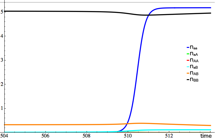
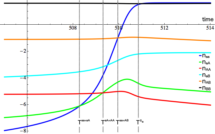
Figure 6. zoom-in when $aa$ recovers, general qualitative behaviour of $\{n_{i}\left(t\right),i\in\mathcal{G}\}$ (lhs) and log-plot (rhs).

Since $aa$ is growing now also out of itself it will influence the sum-process $\Sigma_{5}=n_{aA}+n_{AA}+n_{aB}+n_{AB}+n_{BB}$ and we need new lower bounds on $\Sigma_{5}$ in the following steps, the proof of this works similar to the one of Proposition 4.7 by taking into account all contributing populations. Let us compute the ODE to which $\Sigma_{5}$ is the solution:

Proposition 4.22.

The sum-process $\Sigma_{5}$ is the solution to

$$\dot{\Sigma}_{5}= \Sigma_{5}\left(f-D-{\Delta}-c\Sigma_{5}\right)-{\Delta}\left(n_{aA}+n_{AA}\right)-cn_{aa}\left(n_{aA}+n_{AA}\right)+2\eta n_{aA}n_{BB}$$

$$+{\textstyle{f\over\Sigma_{3}}}n_{aa}\left({\textstyle{1\over 2}}n_{aA}+n_{AA}\right)-{\textstyle{f\over 4\Sigma_{5}}}n_{aB}(n_{aA}+n_{aB})-{\textstyle{f\over 4\Sigma_{6}}}n_{aA}\left(2n_{aa}+n_{aA}+n_{aB}\right).$$ (4.224)

Proof.

We calculate the birth- and the death-rate of $\Sigma_{5}$ under consideration of the $aa$ population:

$$b_{\Sigma_{5}}= {\textstyle{f\over\Sigma_{3}}}n_{aa}\left({\textstyle{1\over 2}}n_{aA}+n_{AA}\right)+{\textstyle{f\over\Sigma_{5}}}\left(\left(n_{aB}+n_{AB}+n_{BB}\right)\Sigma_{5}-{\textstyle{1\over 4}}n_{aB}\left(n_{aA}+n_{aB}\right)\right)$$

$$+\frac{f}{\Sigma_{6}}\left(\left(n_{aA}+n_{AA}\right)\Sigma_{6}-n_{aA}\left({\textstyle{1\over 2}}n_{aa}+{\textstyle{1\over 4}}n_{aA}+{\textstyle{1\over 4}}n_{aB}\right)\right)$$

$$= f\Sigma_{5}+{\textstyle{f\over\Sigma_{3}}}n_{aa}\left({\textstyle{1\over 2}}n_{aA}+n_{AA}\right)-{\textstyle{f\over 4\Sigma_{5}}}n_{aB}\left(n_{aA}+n_{aB}\right)-{\textstyle{f\over 4\Sigma_{6}}}n_{aA}\left(2n_{aa}+n_{aA}+n_{aB}\right),$$ (4.225)

$$d_{\Sigma_{5}}= \Sigma_{5}\left(D-{\Delta}+c\Sigma_{5}\right)+(cn_{aa}+{\Delta})\left(n_{aA}+n_{AA}\right)-2\eta n_{aA}n_{BB},$$ (4.226)

which gives the result. ∎

We introduce some notation for the order of magnitude of $n_{AA}(T_{2})$. We write $n_{AA}(T_{2})={\Theta}({\varepsilon}^{\gamma})$ with

$$\gamma:=2/(1+\eta\bar{n}_{B}-\Delta).$$ (4.227)

Thus the initial condition of the third Phase can be written as:

$$n_{aa}(T_{2}) \leq{\Theta}({\varepsilon}^{2}),$$ (4.228)

$$n_{aA}(T_{2}) ={\Theta}({\delta}n_{AA})={\Theta}({\delta}{\varepsilon}^{\gamma}),$$ (4.229)

$$n_{AA(T_{2})} ={\Theta}({\varepsilon}^{\gamma}),$$ (4.230)

$$n_{aB}(T_{2}) ={\Theta}({\delta}n_{AB})={\Theta}({\delta}{\varepsilon}^{{\gamma}/2}),$$ (4.231)

$$n_{AB}(T_{2}) ={\Theta}({\varepsilon}^{{\gamma}/2}),$$ (4.232)

$$n_{BB}(T_{2}) =\bar{n}_{B}-{\Theta}({\varepsilon}^{{\gamma}/2}),$$ (4.233)

Let

$$T_{3}:=T^{aa}_{\bar{n}_{a}-{\varepsilon}_{0}}=\inf\left\{t>T_{2}:n_{aa}(t)=\bar{n}_{a}-{\varepsilon}_{0}\right\}.$$ (4.234)

We define the stopping time

$$T_{+}:=\min\left\{T_{{\varepsilon}^{\gamma/10}}^{AB},T^{aA=AB},T^{AA=AB}\right\},$$ (4.235)

where:

$$T_{{\varepsilon}^{\gamma/10}}^{AB} :=\inf\left\{t>T_{2}:n_{AB}(t)\geq{\varepsilon}^{\gamma/10}\right\},$$ (4.236)

$$T^{aA=AB} :=\inf\left\{t>T_{2}:n_{aA}(t)=n_{AB}(t)\right\},$$ (4.237)

$$T^{AA=AB} :=\inf\left\{t>T_{2}:n_{AA}(t)=n_{AB}(t)\right\}.$$ (4.238)

Note that for the following arguments, ${\gamma/10}$ can be replaced by any positive power smaller than $\gamma/2$.

We have to ensure that the $aa$ population grows until a neighbourhood of its equilibrium. From Theorem 4.19 and Proposition 4.20, at the end of the second Phase we have that $n_{aA},n_{AA},n_{aB}\leq n_{AB}<{\Delta}$. We start to bound $\Sigma_{5}$:

Lemma 4.23.

For all $t\in[T_{2},T_{+}]$, the sum-process $\Sigma_{5}$ is bounded from above and below by

$$\bar{n}_{B}-{\textstyle{f+3{\Delta}\over c\bar{n}_{B}}}n_{AB}\leq\Sigma_{5}\leq\bar{n}_{B}+{\textstyle{4(f+{\Delta})\over c\bar{n}_{B}}}n_{AB}.$$ (4.239)

Proof.

We use Lemma 4.2 and construct minorising and majorising processes on $\Sigma_{5}$ and $n_{AB}$. First observe that the bounds are satisfied at $t=T_{2}$ by Proposition 4.7. From Proposition 4.22 we can deduce that

$$f\Sigma_{5}-fn_{AB}~{} \leq b_{\Sigma_{5}}\leq f\Sigma_{5}+2fn_{AB},$$ (4.240)

$$\Sigma_{5}(D-{\Delta}+c\Sigma_{5})-(2f+{\Delta})n_{AB} \leq d_{\Sigma_{5}}\leq\Sigma_{5}(D-{\Delta}+c\Sigma_{5})+2(f+{\Delta})n_{AB},$$ (4.241)

$$\Sigma_{5}(f-D+{\Delta}-c\Sigma_{5})-(f+2{\Delta})n_{AB} \leq\dot{\Sigma}_{5}\leq\Sigma_{5}(f-D+{\Delta}-c\Sigma_{5})+(4f+{\Delta})n_{AB}.$$ (4.242)

At the lower bound we get that the sum-process would increase:

$$\dot{\Sigma}_{5}\geq{\Delta}n_{AB}-{\Theta}\left(n_{AB}^{2}\right)>0,$$ (4.243)

and at the upper bound it would decrease:

$$\dot{\Sigma}_{5}\leq-3{\Delta}n_{AB}-{\Theta}\left(n_{AB}^{2}\right)<0.$$ (4.244)

It is left to show that

$$-{\textstyle{(f+3{\Delta})\over c\bar{n}_{B}}}\dot{n}_{AB}\leq\dot{\Sigma}_{5}\leq{\textstyle{4(f+{\Delta})\over c\bar{n}_{B}}}\dot{n}_{AB}.$$ (4.245)

For this we construct a minorising process on $AB$ using that $n_{aA},n_{AA},n_{aB}\leq n_{AB}$, for the birth rate:

$$b_{AB} \geq{\textstyle{f\over\Sigma_{5}}}n_{AB}\left({\textstyle{1\over 4}}n_{aA}+{\textstyle{1\over 2}}n_{AA}+{\textstyle{1\over 2}}n_{aB}+{\textstyle{1\over 2}}n_{AB}+n_{BB}\right)\geq fn_{AB}-{\textstyle{9f\over 4\Sigma_{5}}}n_{AB}^{2},$$ (4.246)

$$d_{AB} \leq n_{AB}(D-{\Delta}+c\Sigma_{5}),$$ (4.247)

$$\dot{n}_{AB} \geq n_{AB}\left(f-D+{\Delta}-c\Sigma_{5}-{\textstyle{9f\over 4\Sigma_{5}}}n_{AB}\right).$$ (4.248)

At the lower bound we have $\dot{n}_{AB}\geq-{\textstyle{5f+12{\Delta}\over 4\bar{n}_{B}}}n_{AB}^{2}+{\Theta}\left(n_{AB}^{3}\right)$.
The lhs of (4.245) $\leq\frac{(5f+12{\Delta})(f+3{\Delta})}{4c\bar{n}_{B}^{2}}n_{AB}^{2}+{\Theta}\left(n_{AB}^{3}\right)<{\Delta}n_{AB}-{\Theta}\left(n_{AB}^{2}\right)$. At the upper bound we get $\dot{n}_{AB}\geq-{\textstyle{25f+16{\Delta}\over 4\bar{n}_{B}}}n_{AB}^{2}-{\Theta}\left(n_{AB}^{3}\right)$ and that the rhs of (4.245) is larger or equal to $-{\textstyle{4(f+{\Delta})(21f+4{\Delta})\over 4c\bar{n}_{B}^{2}}}n_{AB}^{2}-{\Theta}\left(n_{AB}^{3}\right)>-3{\Delta}n_{AB}-{\Theta}\left(n_{AB}^{2}\right)$. ∎

The following lemma ensures that the $aA$- and the $AA$ populations stay smaller than ${\Theta}\left(n_{AB}^{2}\right)$ for all $t\in[T_{2},T_{+}]$:

Lemma 4.24.

1. For all $t\in[T_{2},T_{+}]$, the $AA$ population is bounded from above by

   $$n_{AA}\leq{\textstyle{2\over\bar{n}_{B}}}n_{AB}^{2},$$ (4.249)

2. For all $t\in[T_{2},T_{+}]$ and $\eta<{\textstyle{c\over 2}}\left(1-{\textstyle{{\Theta}({\Delta})\over f-D+{\Delta}}}\right)$, the $aA$ population is bounded from above by

   $$n_{aA}\leq{\textstyle{10f\over\bar{n}_{B}(D-{\Delta})}}n_{AB}^{2}.$$ (4.250)

In particular this implies $T_{+}=T^{AB}_{{\varepsilon}^{\gamma/10}}$.

Proof.

The proof uses again Lemma 4.2. First observe that by Lemma 4.13 (1) and since $n_{aA}(T_{2})={\delta}n_{AA}(T_{2})$ the bounds are satisfied at $t=T_{2}$.

1. We have to show that

   $$\dot{n}_{AA}<{\textstyle{4\over\bar{n}_{B}}}n_{AB}\dot{n}_{AB}.$$ (4.251)

   We construct a majorising process on $n_{AA}$:

   $$b_{AA} \leq{\textstyle{f\over\Sigma_{5}}}n_{AA}(n_{aA}+n_{AA}+n_{AB})+{\textstyle{f\over 4\Sigma_{5}}}(n_{aA}+n_{AB})^{2}.$$ (4.252)

   For the death rate we use Lemma 4.23:

   $$d_{AA} \geq n_{AA}(f-{\Theta}({\Delta})),$$ (4.253)

   $$\dot{n}_{AA} \leq-n_{AA}\left({\textstyle{f\over\Sigma_{5}}}(n_{aB}+n_{BB})-{\Theta}({\Delta})\right)+{\textstyle{f\over\Sigma_{5}}}n_{AB}^{2}.$$ (4.254)

   At the upper bound we thus have: $\dot{n}_{AA}\leq-{\textstyle{f\over\bar{n}_{B}}}n_{AB}^{2}+{\Theta}\left({\Delta}n_{AB}^{2}\right)$.
   We now construct a minorising process on $n_{AB}$. As in (4.246) until $T_{+}$ we have a minoration of the birth rate:

   $$b_{AB} \geq{\textstyle{f\over\Sigma_{5}}}n_{AB}\left({\textstyle{1\over 4}}n_{aA}+{\textstyle{1\over 2}}n_{AA}+{\textstyle{1\over 2}}n_{aB}+{\textstyle{1\over 2}}n_{AB}+n_{BB}\right)\geq fn_{AB}-{\textstyle{9f\over 4\Sigma_{5}}}n_{AB}^{2}.$$ (4.255)

   Using Lemma 4.23 the death rate is given by:

   $$d_{AB} \leq n_{AB}(D-{\Delta}+c\Sigma_{5})\leq fn_{AB}+{\textstyle{4(f+{\Delta})\over\bar{n}_{B}}}n_{AB}^{2},$$ (4.256)

   $$\dot{n}_{AB} \geq-{\textstyle{25f+{\Theta}({\Delta})\over 4\bar{n}_{B}}}n_{AB}^{2}.$$ (4.257)

   Thus the rhs of (4.251) is larger or equal to $-{\textstyle{25f+{\Theta}({\Delta})\over\bar{n}_{B}^{2}}}n_{AB}^{3}$. Since $n_{AB}<{\varepsilon}^{\gamma/10}$ until time $T_{+}$, we indeed have, for ${\varepsilon}$ small enough:

   $$\dot{n}_{AA}\leq-{\textstyle{f\over\bar{n}_{B}}}n_{AB}^{2}+{\Theta}\left({\Delta}n_{AB}^{2}\right)<-{\textstyle{25f+{\Theta}({\Delta})\over\bar{n}_{B}^{2}}}n_{AB}^{3}\leq{\textstyle{4\over\bar{n}_{B}}}n_{AB}\dot{n}_{AB}.$$ (4.258)

2. Similarly to (1) we construct a majorising process on $aA$. For the birth rate we use the result of (1):

   $$b_{aA} \leq{\textstyle{f\over 2\Sigma_{3}}}n_{aa}n_{aA}+{\textstyle{9f\over 2\bar{n}_{B}}}n_{AB}^{2}+{\textstyle{f\over 2\Sigma_{6}}}n_{aa}n_{aA}+{\Theta}({\Delta}n_{AB}^{2}).$$ (4.259)

   Applying Lemma 4.23 we get for the death rate:

   $$d_{aA} \geq n_{aA}\left(f+{\Delta}-\eta\bar{n}_{B}+cn_{aa}-{\Theta}(n_{AB})\right),$$ (4.260)

   $$\dot{n}_{aA} \leq-n_{aA}\left({\textstyle{f\over 2}}-\eta\bar{n}_{B}+{\textstyle{f-2(D-{\Delta})\over 2\Sigma_{5}}}n_{aa}\right)+{\textstyle{9f\over 2\bar{n}_{B}}}n_{AB}^{2}+{\Theta}({\Delta}n_{AB}^{2}),$$ (4.261)

   $$\dot{n}_{aA} \leq-n_{aA}{\textstyle{f-2\eta\bar{n}_{B}\over 2}}+{\textstyle{9f+{\Theta}({\Delta})\over 2\bar{n}_{B}}}n_{AB}^{2}.$$ (4.262)

   At the upper bound we get: $\dot{n}_{aA}\leq n_{AB}^{2}\left({\textstyle{9f+{\Theta}({\Delta})\over 2\bar{n}_{B}}}-{\textstyle{10f(f-2\eta\bar{n}_{B})\over 2\bar{n}_{B}(D-{\Delta})}}\right)$. We will show that

   $$\dot{n}_{aA}\leq{\textstyle{20f\over\bar{n}_{B}(D-{\Delta})}}n_{AB}\dot{n}_{AB}.$$ (4.263)

   For this we use the minorising process on $AB$ constructed in (4.257), given by $\dot{n}_{AB}\geq-{\textstyle{25f+{\Theta}({\Delta})\over 4\bar{n}_{B}}}n_{AB}^{2}$. Thus the rhs of (4.263) is larger or equal to $-{\textstyle{105f+{\Theta}({\Delta})\over\bar{n}_{B}(D-{\Delta})}}n_{AB}^{3}.$ Thus we have to ensure that $\left({\textstyle{9f+{\Theta}({\Delta})\over 2\bar{n}_{B}}}-{\textstyle{10f(f-2\eta\bar{n}_{B})\over 2\bar{n}_{B}(D-{\Delta})}}\right)<-{\textstyle{105f+{\Theta}({\Delta})\over\bar{n}_{B}(D-{\Delta})}}{\Delta}$. This yields the condition on $\eta$:

   $$\eta\leq{\textstyle{f-D-{\Theta}({\Delta})\over 2\bar{n}_{B}}}={\textstyle{c\over 2}}\left(1-{\textstyle{{\Theta}({\Delta})\over f-D+{\Delta}}}\right).$$ (4.264)

∎

Remark.

Observe that the condition $\eta<{\textstyle{c\over 2}}\left(1-{\textstyle{{\Theta}({\Delta})\over f-D+{\Delta}}}\right)$ in Lemma 4.24 prevents $aA$ to grow exponentially fast. Inequality (4.261) shows that for larger values for $\eta$, $n_{aA}$ would start to grow out of itself and thus the system would converge towards the 6-point equilibrium as we checked numerically. Hence, the assumption $\eta<{\textstyle{c\over 2}}\left(1-{\textstyle{{\Theta}({\Delta})\over f-D+{\Delta}}}\right)$ is essential in this phase and propagates to the following lemmata since we need therein the $n_{AB}^{2}$-dependent bound on $aA$.

Using Lemma 4.24 we can also compute a lower bound for $AA$:

Lemma 4.25.

For $\eta\leq{\textstyle{c\over 2}}-{\Theta}({\Delta})$ and $t\in[T_{2},T_{+}]$, the $AA$ population is bounded from below by

$${\textstyle{1\over 8\bar{n}_{B}}}n_{AB}^{2}\leq n_{AA}.$$ (4.265)

Proof.

By Lemma 4.2 we construct a minorising process on $AA$ using Lemma 4.23 for the death rate. The bound is satisfied at $t=T_{2}$ by Lemma 4.13 (2).

$$b_{AA} \geq{\textstyle{f\over 4\Sigma_{5}}}n_{AB}^{2},$$ (4.266)

$$d_{AA} \leq n_{AA}(D+c\Sigma_{5}+cn_{aa}),$$ (4.267)

$$\dot{n}_{AA} \geq-n_{AA}\left(f+{\Delta}+{\textstyle{4(f+{\Delta})\over\bar{n}_{B}}}n_{AB}+cn_{aa}\right)+{\textstyle{f\over 4\Sigma_{5}}}n_{AB}^{2}.$$ (4.268)

At the lower bound we have $\dot{n}_{AA}\geq{\textstyle{D-{\Theta}({\Delta})\over 8\bar{n}_{B}}}n_{AB}^{2}={\Theta}(n_{AB}^{2})$. It is left to show that

$$\dot{n}_{AA}\geq{\textstyle{1\over 4\bar{n}_{B}}}n_{AB}\dot{n}_{AB}.$$ (4.269)

We construct a majorising process on $AB$:

$$b_{AB} \leq{\textstyle{f\over\Sigma_{5}}}(n_{aA}+2n_{AA}+n_{AB})\left({\textstyle{1\over 2}}n_{aB}+{\textstyle{1\over 2}}n_{AB}+n_{BB}\right)$$

$$\leq{\textstyle{f\over\Sigma_{5}}}n_{AB}\left({\textstyle{1\over 2}}n_{aA}+n_{AA}+{\textstyle{1\over 2}}n_{aB}+{\textstyle{1\over 2}}n_{AB}+n_{BB}\right)+f(n_{aA}+2n_{AA})$$

$$\leq fn_{AB}+f(n_{aA}+2n_{AA})-{\textstyle{f\over 4\Sigma_{5}}}n_{AB}^{2}.$$ (4.270)

For the death rate we use Lemma 4.23:

$$d_{AB} \geq n_{AB}\left(f-{\textstyle{(f+3{\Delta})\over\bar{n}_{B}}}n_{AB}\right),$$ (4.271)

$$\dot{n}_{AB} \leq{\textstyle{3f+12{\Delta}\over\bar{n}_{B}}}n_{AB}^{2}+f(n_{aA}+2n_{AA}).$$ (4.272)

Using Lemma 4.24 we get that the rhs of (4.269) is smaller or equal to ${\textstyle{f\over 4\bar{n}_{B}}}n_{AB}n_{aA}+{\Theta}\left(n_{AB}^{3}\right)\leq{\Theta}\left(n_{AB}^{3}\right)<{\Theta}(n_{AB}^{2})$ for ${\varepsilon}$ small enough since $n_{AB}\leq{\varepsilon}^{\gamma/10}$ for $t\in[T_{2},T_{+}]$. ∎

With all these lemmata we are now able to show that $n_{AB}$ stays below ${\varepsilon}^{\gamma/10}$ until $T_{3}$ when $n_{aa}$ reaches the neighbourhood of its equilibrium.

Lemma 4.26.

For $t\in[T_{2},T_{+}]$, it holds

$$T_{+}=T_{{\varepsilon}^{\gamma/10}}^{AB}\geq{\Theta}\left({\varepsilon}^{-{\gamma}/2}\right).$$ (4.273)

Proof.

As in (4.270) we construct a majorising process on $AB$ using Lemma 4.24:

$$b_{AB} \leq fn_{AB}+f(n_{aA}+2n_{AA})-{\textstyle{f\over 4\Sigma_{5}}}n_{AB}^{2},$$

$$\leq fn_{AB}+{\Theta}\left(n_{AB}^{2}\right).$$ (4.274)

By Lemma 4.23 the death rate can be bounded by:

$$d_{AB} \geq fn_{AB}-{\Theta}\left(n_{AB}^{2}\right),$$ (4.275)

$$\dot{n}_{AB} \leq{\Theta}\left(n_{AB}^{2}\right).$$ (4.276)

With the initial condition $n_{AB}(T_{2})={\Theta}\left({\varepsilon}^{\gamma/2}\right)$, we get the upper bound

$$n_{AB}(t)\leq\frac{{\Theta}(1)}{{\Theta}\left({\varepsilon}^{-{\gamma}/2}\right)-{\Theta}(1)t}.$$ (4.277)

Thus $T_{{\varepsilon}^{\gamma/10}}^{AB}\geq{\Theta}\left({\varepsilon}^{-{\gamma}/2}\right)$. Observe that it follows that $T_{{\varepsilon}^{\gamma/5}}^{AA}={\Theta}({\varepsilon}^{-{\gamma}/2})$. ∎

To ensure the exponential growth of $aa$ we need that the $aA$ population does not decay under the order ${\Theta}({\varepsilon}^{\gamma})$.

Lemma 4.27.

For $\eta\leq{\textstyle{c\over 2}}-{\Theta}({\Delta})$ and for all $t\in[T_{2},T_{2}+{\Theta}({\varepsilon}^{-\gamma/2})]$, if $n_{aa}\leq n_{AB}$, then

$$n_{aA}\geq{\Theta}\left(\delta n_{AB}^{2}\right).$$ (4.278)

Proof.

We construct a minorising process on $aA$ in a very rough way assuming that there is no birth. Since $n_{aa}\leq n_{AB}$ the death rate can be bounded by using Lemma 4.23:

$$d_{aA} \leq n_{aA}(f+\Delta+cn_{aa}+{\Theta}(n_{AB}))$$

$$\leq n_{aA}(f+{\Delta}+{\Theta}(n_{AB})).$$ (4.279)

By Lemma 4.24 we get:

$$\dot{n}_{aA}\geq-{\Theta}\left(n_{AB}^{2}\right).$$ (4.280)

At time $T_{2}$ we know that $n_{aA}=\delta n_{AA}={\Theta}\left(\delta n_{AB}^{2}\right)={\Theta}(\delta{\varepsilon}^{\gamma})$. Thus, using (4.277) to bound $n_{AB}$, we conclude that $n_{aA}$ satisfies until $T_{+}$:

$$n_{aA}(t)\geq{\frac{{\Theta}(1)}{{\Theta}(1)t-{\Theta}({\varepsilon}^{-\gamma/2})}+{\Theta}(\delta{\varepsilon}^{\gamma})+{\Theta}({\varepsilon}^{\gamma/2}).}$$ (4.281)

We have to ensure that the slope of a minorising process on $AB$ is of the same order. Thus we construct a minorising process on $AB$ using Lemma 4.24 and that $n_{aa}\leq n_{AB}$:

$$b_{AB} \geq{\textstyle{f\over\Sigma_{5}}}n_{AB}\left({\textstyle{1\over 2}}n_{aA}\!+\!n_{AA}\!+\!{\textstyle{1\over 2}}n_{aB}\!+\!{\textstyle{1\over 2}}n_{AB}\!+\!n_{BB}\right)\!+\!{\textstyle{f\over\Sigma_{6}}}(n_{aA}\!+\!2n_{AA})\left({\textstyle{1\over 2}}n_{aB}\!+\!{\textstyle{1\over 2}}n_{AB}\!+\!n_{BB}\right)\!-\!{\Theta}\left(n_{AB}^{3}\right)$$

$$\geq fn_{AB}-{\textstyle{f\over\Sigma_{5}}}n_{AB}^{2}-{\Theta}\left(n_{AB}^{3}\right).$$ (4.282)

where for the last inequality we used that $n_{aB}\leq n_{AB}$. Using Lemma 4.23 we get:

$$d_{AB} \leq n_{AB}(f+{\Theta}(n_{AB})),$$ (4.283)

$$\dot{n}_{AB} \geq-{\Theta}(n_{AB}^{2}).$$ (4.284)

Thus the minorising process on $AB$ is given by:

$$n_{AB}(t)\geq{\frac{{\Theta}(1)}{{\Theta}(1)t+{\Theta}({\varepsilon}^{-\gamma/2})}}$$ (4.285)

The minorising process (4.285) stays of order ${\Theta}({\varepsilon}^{\gamma/2})$ during a time of order ${\Theta}({\varepsilon}^{-\gamma/2})$.
The minorising process (4.281) needs time of order ${\Theta}\left({\varepsilon}^{-\gamma/2}\right)$, to reach the order ${\Theta}\left(\delta{\varepsilon}^{\gamma+\alpha}\right)$ for any $\alpha>0$. The bound (4.278) is thus ensured for a time of order ${\Theta}({\varepsilon}^{-\gamma/2})$. ∎

Now we show that $n_{aa}$ increases to a neighbourhood of its equilibrium before time $T_{+}$.

Lemma 4.28.

For $\eta\leq{\textstyle{c\over 2}}-{\Theta}({\Delta})$ and all $t\in[T_{2},T_{+}]$ the $aa$ population increases to a ${\varepsilon}_{0}$-neighbourhood of its equilibrium $\bar{n}_{a}$ exponentially fast, and $T_{3}<T_{+}$.

Proof.

We construct a minorising process on $aa$ and distinguish some cases. We remember that $n_{aa}(T_{2})={\Theta}({\varepsilon}^{2})$ if we do not have a better starting value. First observe that by Lemma 4.24 it holds that $d_{aa}\leq n_{aa}\left(D+{\Delta}+cn_{aa}+{\Theta}\left(n_{AB}^{2}\right)\right)$.

1. If $n_{aa}\leq n_{aA}\leq n_{AA}$ or $n_{aA}\leq n_{aa}\leq n_{AA}$
   In that case the birth-rate is given by $b_{aa}\geq fn_{aa}{\textstyle{n_{aA}\over 6n_{AA}}}$. With Lemma 4.24 and 4.27 we get $b_{aa}\geq{\Theta}({\delta})fn_{aa}$ and $\dot{n}_{aa}\geq n_{aa}\left({\Theta}({\delta})f-D-{\Delta}-{\Theta}\left(n_{AB}^{2}\right)\right)$.
   Hence the time until $aa$ reaches $\bar{n}_{a}-{\varepsilon}_{0}$ satisfies $T_{3}\leq{\Theta}\left(\ln({\varepsilon}^{-2})\right)={\Theta}(\ln(1/{\varepsilon}))$.

2. If $n_{aa},n_{AA}\leq n_{aA}$
   In that case, by Lemma 4.24 we get $b_{aa}\geq{\textstyle{f\over 6}}n_{aa}$ and $\dot{n}_{aa}\geq n_{aa}\left({\textstyle{f\over 6}}\!-\!D\!-\!{\Delta}\!-\!{\Theta}\left(n_{AB}^{2}\right)\!\right)$.
   Hence $T_{3}\leq{\Theta}\left(\ln\left({\varepsilon}^{-2}\right)\right)={\Theta}(\ln(1/{\varepsilon}))$.

3. If $n_{aA}\leq n_{AA}\leq n_{aa}\leq n_{AB}$
   In that case, by Lemma 4.24, $b_{aa}\geq{\textstyle{f\over 3}}n_{aa}$ and $\dot{n}_{aa}\geq n_{aa}\!\left({\textstyle{f\over 3}}\!-\!D\!-\!{\Delta}\!-\!cn_{aa}\!-\!{\Theta}\!\left(n_{AB}^{2}\right)\!\right)$. Hence $T_{3}\leq{\Theta}\left(\ln\left({\varepsilon}^{-{\gamma}/5}\right)\right)={\Theta}(\ln(1/{\varepsilon}))$.

4. If $n_{AA}\leq n_{aA}\leq n_{aa}\leq n_{AB}$
   In that case, by Lemma 4.24, $b_{aa}\geq{\textstyle{f\over 3}}n_{aa}$ and $\dot{n}_{aa}\!\geq n_{aa}\!\left({\textstyle{f\over 3}}\!-\!D\!-\!{\Delta}\!-\!cn_{aa}\!-\!{\Theta}\left(n_{AB}^{2}\right)\!\right)$. Hence $T_{3}\leq{\Theta}\left(\ln\left({\varepsilon}^{-{\gamma}/5}\right)\right)={\Theta}(\ln(1/{\varepsilon}))$.

5. If $n_{aa}>n_{AB}$
   In that case, by Lemma 4.24, $b_{aa}\geq n_{aa}(f-{\Theta}({n_{AB}^{2}}/{n_{aa}}))$ and $\dot{n}_{aa}\geq n_{aa}(f-D-{\Delta}-cn_{aa}-{\Theta}({n_{AB}^{2}}/{n_{aa}}))$. Hence $T_{3}\leq{\Theta}({\varepsilon}^{{\gamma}/10}\ln({\varepsilon}^{-{\gamma}/10}))={\Theta}({\varepsilon}^{\gamma/10}\ln(1/{\varepsilon}))$.

Thus, remembering Lemma 4.26, we proved that $T_{3}\leq{\Theta}(\ln(1/{\varepsilon}))\leq{\Theta}({\varepsilon}^{-\gamma/2})\leq T_{+}.$ ∎

4.5. Phase 4: Convergence to $p_{aB}=(\bar{n}_{a},0,0,0,0,\bar{n}_{B})$

The Jacobian matrix of the field (2.25) at the fixed point $p_{aB}$ has the 6 eigenvalues: $0$ (double), and $-(2f-D),-(f-D+\Delta),-(f-D-\Delta),-((f-D)(5f-4D)+f\Delta)/(4(f-D)+\eta\bar{n}_{B})$ which are strictly negative under Assumptions (C). Because of the zero eigenvalues, $p_{aB}$ is a non-hyperbolic equilibrium point of the system and linearisation fails to determine its stability properties. Instead, we use the result of the center manifold theory [20, 28] that asserts that the qualitative behaviour of the dynamical system in a neighbourhood of the non-hyperbolic critical point $p_{aB}$ is determined by its behaviour on the center manifold near $p_{aB}$.

Theorem 4.29 (The Local Center Manifold Theorem 2.12.1 in [28]).

Let $f\in C^{r}(E)$, where $E$ is an open subset of ${\mathbb{R}}^{n}$ containing the origin and $r\geq 1$. Suppose that $f(0)=0$ and $Df(0)$ has $c$ eigenvalues with zero real parts and $s$ eigenvalues with negative real parts, where $c+s=n$. Then the system $\dot{z}=f(z)$ can be written in diagonal form

$$\dot{x} =Cx+F(x,y),$$ (4.286)

$$\dot{y} =Py+G(x,y),$$ (4.287)

where $z=(x,y)\in{\mathbb{R}}^{c}\times{\mathbb{R}}^{s}$, $C$ is a $c\times c$-matrix with $c$ eigenvalues having zero real parts, $P$ is a $s\times s$-matrix with $s$ eigenvalues with negative real parts, and $F(0)=G(0)=0,DF(0)=DG(0)=0.$ Furthermore, there exists $\delta>0$ and a function, $h\in C^{r}(N_{\delta}(0))$, where $N_{\delta}(0)$ is the ${\delta}$-neighbourhood of $0$, that defines the local center manifold and satisfies:

$$Dh(x)[Cx+F(x,h(x))]-Ph(x)-G(x,h(x))=0,$$ (4.288)

for $|x|<{\delta}$. The flow on the center manifold $W^{c}(0)$ is defined by the system of differential equations

$$\dot{x}=Cx+F(x,h(x)),$$ (4.289)

for all $x\in{\mathbb{R}}^{c}$ with $|x|<{\delta}$.

Theorem 4.30.

The non-hyperbolic critical point $p_{aB}$ is a stable fixed point and the flow on the center manifold near the critical point approaches $p_{aB}$ with speed $\frac{1}{t}$.

Proof.

We apply the Local Center Manifold Theorem 4.29. All the calculations below were done with the program Mathematica 11.0.0.0 Student Edition. We do not write the results of all the intermediary calculations as they would take a few pages and bring no more information. Instead, we describe as precisely as possible the calculations we did so that they can be checked by the reader (using a similar computer program).

By the affine transformation $(n_{aa},n_{BB})\mapsto(n_{aa}-\bar{n}_{a},n_{BB}-\bar{n}_{B})$ we get a translated system $\tilde{F}(n)$ which has a critical point at the origin. We compute the two eigenvectors corresponding to 0 eigenvalues of the Jacobian matrix of $\tilde{F}$ at the fixed point $(0,0,0,0,0,0)$, which are

$$EV_{1}=(0,0,0,1,0,-1)\quad and\quad EV_{2}=(0,0,0,-1,1,0).$$ (4.290)

We perform a new change of variable to work in the basis of eigenvectors of $\tilde{F}(n)$. Let us call the new coordinates $x_{1},\ldots,x_{6}$. Let $h(x_{1},x_{2})$ be the local center manifold (still unknown). We shall look at its local shape near $(0,0)$ and expand it up to second order. Let us write

$$h(x_{1},x_{2})=\begin{pmatrix}{\lambda_{3}}x_{1}^{2}+{\nu_{3}}{x_{1}}{x_{2}}+{\mu_{3}}x_{2}^{2}\\ {\lambda_{4}}x_{1}^{2}+{\nu_{4}}{x_{1}}{x_{2}}+{\mu_{4}}x_{2}^{2}\\ {\lambda_{5}}x_{1}^{2}+{\nu_{5}}{x_{1}}{x_{2}}+{\mu_{5}}x_{2}^{2}\\ {\lambda_{6}}x_{1}^{2}+{\nu_{6}}{x_{1}}{x_{2}}+{\mu_{6}}x_{2}^{2}\end{pmatrix}+O\left(x^{3}\right).$$ (4.291)

We then substitute the series expansions into the center manifold equation (4.288) which gives us 12 equations for the 12 unknowns $\lambda_{3},\ldots,\mu_{6}$. Substitution of the explicit second order approximation of the center manifold equation into (4.289) yields the (order 2 approximation of the) flow on the local center manifold:

$$\dot{x}_{1} =\frac{A_{1}}{B_{1}}{x_{1}}{x_{2}}+\frac{C_{1}}{D_{1}}{x_{2}}^{2}+\frac{E_{1}}{F_{1}}{x_{1}}^{2}+O\left(x^{3}\right),$$ (4.292)

$$\dot{x}_{2} =\frac{A_{2}}{B_{2}}{x_{1}}{x_{2}}+\frac{C_{2}}{D_{2}}{x_{2}}^{2}+\frac{E_{2}}{F_{2}}{x_{1}}^{2}+O\left(x^{3}\right),$$ (4.293)

where we obtain

$$A_{1} =3c^{2}Df^{2}-c^{2}{\Delta}f^{2}-3c^{2}f^{3},$$ (4.294)

$$B_{1} =(D-{\Delta}-f)\left(4cD^{2}-9cDf+c{\Delta}f+5cf^{2}-4D^{2}{\eta}+4D{\Delta}{\eta}+8D{\eta}f-4{\Delta}{\eta}f-4{\eta}f^{2}\right),$$ (4.295)

$$C_{1} =12c^{2}D^{3}f^{2}-4c^{2}D^{2}{\Delta}f^{2}-39c^{2}D^{2}f^{3}+12c^{2}D{\Delta}f^{3}+42c^{2}Df^{4}-c^{2}{\Delta}^{2}f^{3}-8c^{2}{\Delta}f^{4}$$

$$\quad-15c^{2}f^{5}+12cD^{3}{\eta}f^{2}-16cD^{2}{\Delta}{\eta}f^{2}-36cD^{2}{\eta}f^{3}+4cD{\Delta}^{2}{\eta}f^{2}+32cD{\Delta}{\eta}f^{3}$$

$$\quad+36cD{\eta}f^{4}-4c{\Delta}^{2}{\eta}f^{3}-16c{\Delta}{\eta}f^{4}-12c{\eta}f^{5},$$ (4.296)

$$D_{1} =8(D-2f)(D-f)(D-{\Delta}-f)\times$$

$$\quad\times\left(4cD^{2}-9cDf+c{\Delta}f+5cf^{2}-4D^{2}{\eta}+4D{\Delta}{\eta}+8D{\eta}f-4{\Delta}{\eta}f-4{\eta}f^{2}\right),$$ (4.297)

$$E_{1} =cf,\quad F_{1}=2(-D+{\Delta}+f),$$ (4.298)

and

$$A_{2} =2c^{2}D^{2}f-3c^{2}Df^{2}+c^{2}f^{3}-2cD^{2}{\eta}f+2cD{\Delta}{\eta}f+4cD{\eta}f^{2}-2c{\Delta}{\eta}f^{2}-2c{\eta}f^{3},$$ (4.299)

$$B_{2} =(D-{\Delta}-f)\left(4cD^{2}-9cDf+c{\Delta}f+5cf^{2}-4D^{2}{\eta}+4D{\Delta}{\eta}+8D{\eta}f-4{\Delta}{\eta}f-4{\eta}f^{2}\right),$$ (4.300)

$$C_{2} =-3cD{\eta}f^{2}+c{\Delta}{\eta}f^{2}+3c{\eta}f^{3},$$ (4.301)

$$D_{2} =2(D-2f)\left(4cD^{2}-9cDf+c{\Delta}f+5cf^{2}-4D^{2}{\eta}+4D{\Delta}{\eta}+8D{\eta}f-4{\Delta}{\eta}f-4{\eta}f^{2}\right),$$ (4.302)

$$E_{2} =0,\quad F_{2}=1.$$ (4.303)

It is left to show that the above system flows toward the origin, at least for $\eta$ smaller than a certain constant. To do that, we perform another change of variables which allows us to work in the positive quadrant. We call the new coordinates (on the center manifold) $y_{1}$ and $y_{2}$, and the new field $\hat{F}$. Observe that it is sufficient to prove that the scalar product of the field with the position is negative. We thus consider the function

$$s(y_{1},y_{2})=\left(\hat{F}(y_{1},y_{2}),(y_{1},y_{2})\right),$$ (4.304)

which is a quadratic form in $y_{1}$ and $y_{2}$. As the field $\hat{F}$ is homogeneous of degree 2 in its variables, it is enough to consider any direction given by $y_{2}=\lambda y_{1}$, and prove that $s(y_{1},\lambda y_{1})<0$ for all $\lambda>0$. As the expressions are so ugly, we work perturbatively in $f$ and consider it as large as needed. Observe that the numerator and the denominator of $s(y_{1},\lambda y_{1})$ are polynomials of degree 5 in $f$. We thus compute the coefficient in front of $f^{5}$, and obtain by a series expansion:

$$s(y_{1},\lambda y_{1})=\frac{c{y_{1}}^{3}\left(c\left(16\lambda^{3}+7\lambda^{2}+16\lambda+40\right)-4{\eta}\left(5\lambda^{3}+8\lambda^{2}+8\lambda+8\right)\right)}{64{\eta}-80c}f^{5}+{\Theta}\left(f^{4}\right).$$ (4.305)

Observe that the denominator is always negative (because by the assumption that $\eta\leq c$). We finally compute the minimal value of the ratio

$${r}(\lambda)\text{:=}\frac{16\lambda^{3}+7\lambda^{2}+16\lambda+40}{4\left(5\lambda^{3}+8\lambda^{2}+8\lambda+8\right)},$$ (4.306)

and obtain $r_{max}\simeq 0.593644$. Thus, asymptotically as $f\to\infty$, the field is attractive for $\eta<c\cdot r_{max}$. Thus we see that $p_{aB}$ is a stable fixed point which is approached with speed $\frac{1}{t}$ as long as $\eta<c\cdot r_{max}$.
Figure 7 shows the flow in the center manifold of the fixed point $p_{aB}$, for two values of $\eta$, one below the threshold $cr_{max}$ and one above. We see that the flow is attractive in the first case and repulsive in the second one. ∎

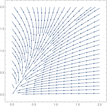
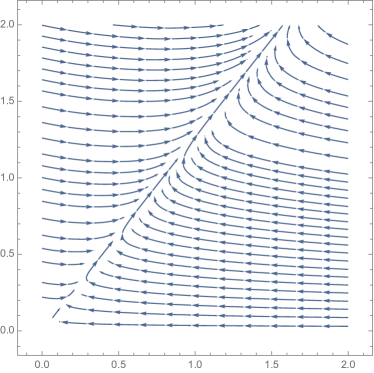
Figure 7. Flow of the dynamical system in the center manifold of the fixed point $p_{aB}$, for $\eta=0.02$ (left) and $\eta=0.6$ (right).

5. Discussion

In the rigorous results we have presented in this paper, we made some particular assumptions on the parameters of our model in order to simplify the analysis of the (already difficult) dynamical system. In this section we discuss which of these assumptions can be relaxed, based on heuristic considerations and numerical simulations.

The no-reproduction-small-competition model.

In the model considered so far, we assume that the mutation to the $B$ allele produces a new species different to the one of phenotype $a$. This is done by the no reproduction assumption between individuals of phenotype $a$ and of phenotype $B$.

These requirements are not needed to observe the recovery of the $aa$ population. In fact, what we require is that the invasion fitness of the $aa$ population into a resident $BB$ population is positive. Therefore, we can relax the no-competition assumption and add a small competition, $c_{aB}$, between $aa$ individuals and $BB$ individuals. This additional competition increases the time until $aa$ can reinvade and also modify the two- population fixed point $p_{aB}$ (see Figure 8).

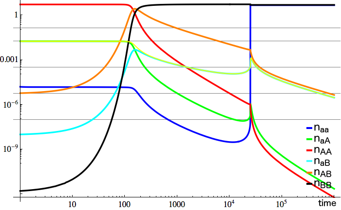
Figure 8. Numerical solution of the deterministic process, loglogplot for $\eta=0$ and $c_{aB}=0.1$.

Adding the factor $\eta$ accelerates the process of recovery, and, consequently, allows to increase the competition rate $c_{aB}$ (see Figure 9).

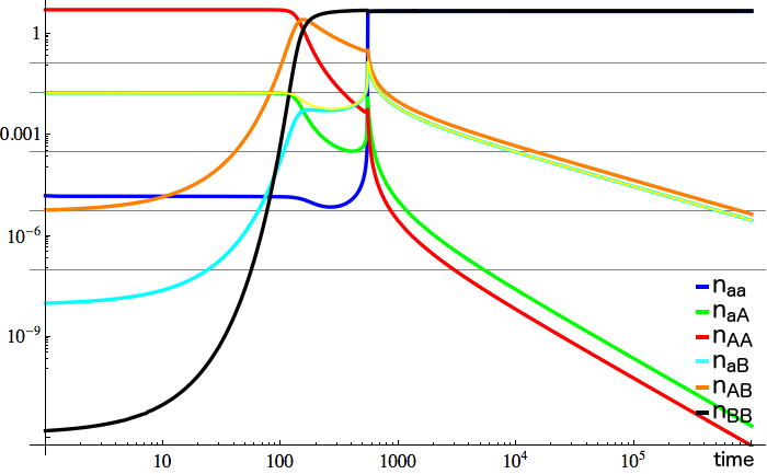
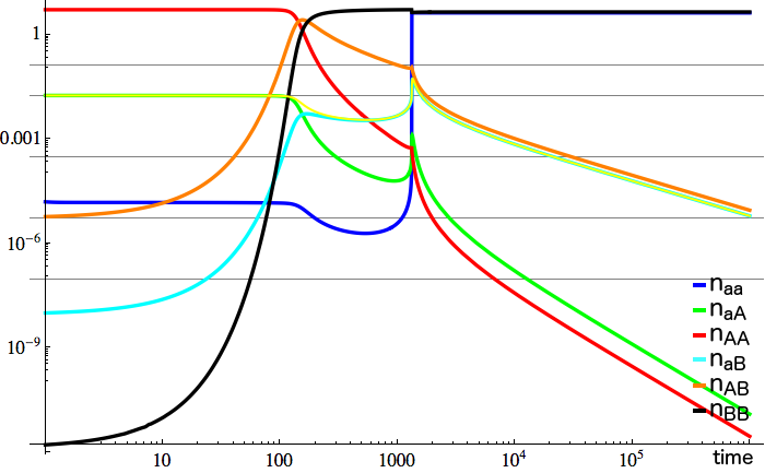
Figure 9. Numerical solution of the deterministic process, loglog-plot (left) for $\eta=0.01$ and $c_{aB}=0.1$, (right) for $\eta=0.01$ and $c_{aB}=0.2$.

For small $\eta$ we end up in a $aa$-$BB$ equilibrium, but by accelerating (increasing $\eta$ or decreasing $c_{aB}$) the process even more, we can also end up in a 6-point equilibrium (all six population coexist) (see Figure 10).

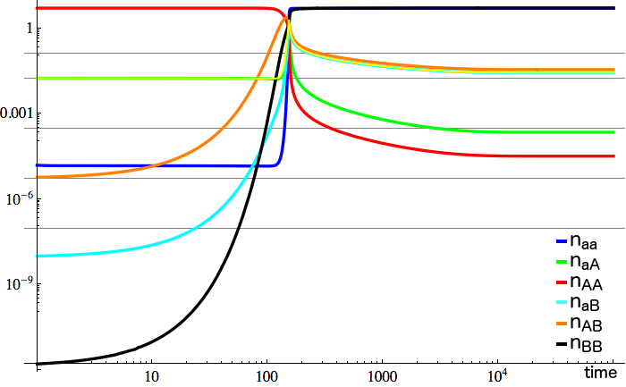
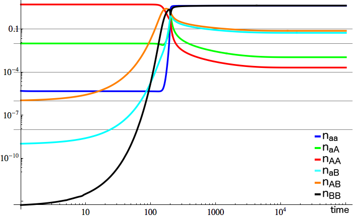
Figure 10. Numerical solution of the deterministic process, loglog-plot (left) for $\eta=0.56$ and $c_{aB}=0$, (right) for $\eta=0.17$ and $c_{aB}=0.2$.

If there is competition between individuals of phenotype $a$ and of phenotype $B$ ($c_{aB}>0$) the $aa$ and $BB$ populations have smaller equilibria as the no-competition equilibria $\bar{n}_{a}$ and $\bar{n}_{B}$, obtained when $c_{aB}=0$. Thus the competition felt from $aA$ by $aa$ and $BB$ is lower and a smaller $\eta$ is enough to observe the 6-point equilibrium.

The all-with-all model.

The assumption of no reproduction between individuals of phenotype $a$ and of phenotype $B$ is also not really necessary for the recovery of the $aa$ population. Let us discuss the all-with-all model where all phenotypes can reproduce among themselves, that is, where the reproductive compatibility is $R_{i}(j)=1$, for all $i,j\in\mathcal{G}$.

If we analyse the invasion fitness of the $aa$ population in the macroscopic $BB$ population, it is positive (and we can observe the recovery of $aa$) if the fecundity $f$ scales with ${\varepsilon}$ in such a way that $f\cdot{\varepsilon}^{2}>D+\Delta$. Indeed, in this model the whole population acts as potential partner for each individual, and the birth rate of $aa$ scales with $\Sigma_{6}$ instead of $\Sigma_{3}$.

If this requirement on $f$ is fulfilled, then numerical simulations show that most of the results carry over to this model, but with the main difference that the 2-points equilibrium is replaced by a 3-points equilibrium. The reason for this is that the reproduction between $a$ and $B$ individuals will always give birth to $aB$ individuals and thus the $aB$ population also survives (see Figure 11 (up)).

We can also add a small competition between individuals of phenotype $a$ and individuals of phenotype $B$ and still get the 3-point equilibrium (see Figure 11(up)).

As in the no-reproduction model, adding the factor $\eta$ results in accelerating the process (see Figure 11 (middle-left)).

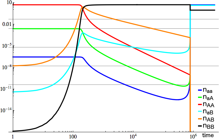
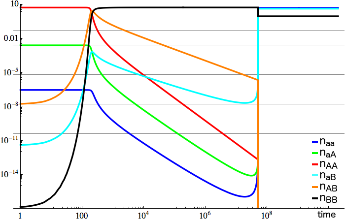
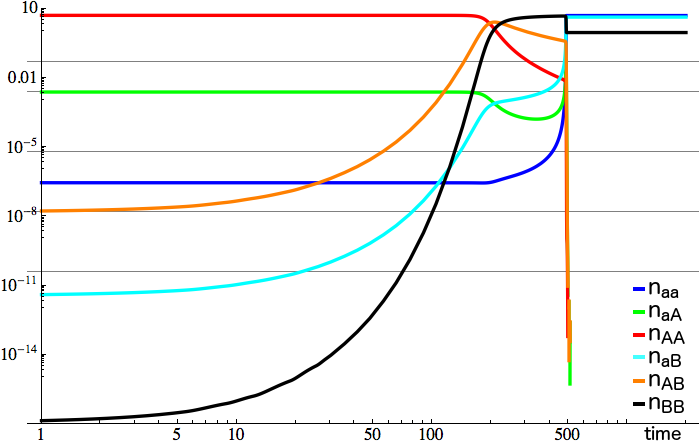
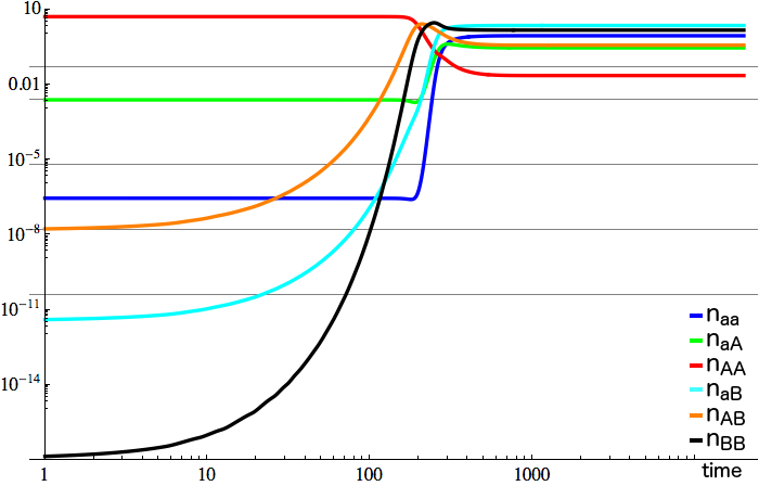
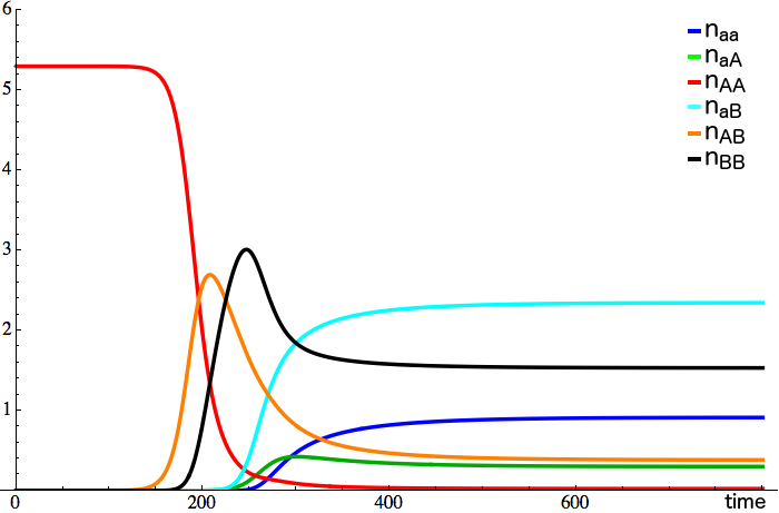
Figure 11. Numerical solution of the all-with-all deterministic process, loglog-plot: (up-left) for $f=6$, $\eta=0$ and $c_{aB}=0$, (up-right) for $f=6$, $\eta=0$ and $c_{aB}=0.05$; (middle-left) for $\eta=0.02$ and $c_{aB}=0$, (middle-right) for $\eta=0$, $c_{aB}=0$ and $f=3$; (down-left) for $\eta=0.17$ and $c_{aB}=0.925$, (down-right) rescaled individual plot for $\eta=0.17$ and $c_{aB}=0.925$.

With reasonable choices for $\eta$ and $c_{aB}$, we end up in a 6-point-equilibrium where all populations coexist (see Figure 11 (down)). Observe, the $aB$ population can be bigger than the $AB$ population, because it gets an additional birth factor from the reproduction of individuals of genotype $aa$ with individuals of phenotype $B$ which outcompetes the birth of $AB$ individuals by reproduction of individuals of genotype $AA$ and of phenotype $B$.

A. Appendix

We collect in this appendix all the important definitions of times separating phases or subphases of the process, and provide a proof summary with all the implications. Recall Definition 4.1, and Figures 4 and 6. We write $N_{\delta}(x)$ for the $\delta$-neighbourhood of $x\in{\mathbb{R}}^{6}$. We consider

$${\Delta}>\delta>{\varepsilon}_{0}>{\varepsilon}>0.$$ (A.1)

and

$T_{1}$	$:=T_{{\varepsilon}_{0}}^{aa+aA+aB+AB+BB}$,
$T_{=}$	$:=T^{aA=aB}$,
$T_{2}$	$:=T^{aA=\delta AA}\land T^{aB=\delta AB}\land T^{aa=aA\wedge aB}$,
$T_{3}$	$:=T^{aa}_{\bar{n}_{a}-{\varepsilon}^{{\gamma}/2}}$.

where $\gamma:=2/(1+\eta\bar{n}_{B}-\Delta)$ is the order of magnitude of $n_{AA}$ at $T_{2}$ : $n_{AA}(T_{2})={\Theta}({\varepsilon}^{\gamma})$.
We summarise below the detailed structure of the proof (we abbreviate Lemma, Proposition and Theorem by L,P, and T respectively):

1. $t\in[0,T_{1}]$
   Initial conditions : $(n_{aa},n_{aA},n_{AA},n_{aB},n_{AB},n_{BB})=({\Theta}({\varepsilon}^{2}),{\varepsilon},\bar{n}_{A}\pm{\Theta}({\varepsilon}),0,{\varepsilon}^{3},0)$.
   With those initial conditions the following bounds hold:

   $$n_{AA}\leq\bar{n}_{A},\quad n_{BB}\leq\bar{n}_{B},\quad n_{aB}\leq n_{AB}\quad\text{(Proposition \ref{aB<AB}) }$$

   Here are the main steps of the proof of Propostion 4.4 and Corollary 4.5. Until the time $T_{1}$,

   $$\text{(P\ref{aB<AB})}\Rightarrow\quad n_{BB}\leq n_{AB}^{2}\quad\text{(1)}$$

   $$\text{(1)}\Rightarrow\quad n_{aB}\leq n_{aA}n_{AB}\quad\text{(2)}$$

   $$\text{(1)(2)}\Rightarrow\quad n_{aa}\leq n_{aA}^{2}\quad\text{(3)}$$

   $$\text{(1)(2)(3)}\Rightarrow\quad T_{1}=T^{AB}_{{\varepsilon}_{0}}={\Theta}(\log({\varepsilon}_{0}/{\varepsilon}^{3})^{1/(\Delta-{\Theta}({\varepsilon}_{0}))})\quad\text{(Proposition \ref{prop-bounds})}$$

   $$\text{(P\ref{prop-bounds})}\Rightarrow\quad \dot{n}_{AB}={\Theta}(\Delta)n_{AB}\quad\text{(Corollary \ref{phase1}(1))}$$

   $$\text{(P\ref{prop-bounds})}\Rightarrow\quad \bar{n}_{A}-{\Theta}({\varepsilon})\leq\Sigma_{5}\leq\bar{n}_{A}+2\Delta{\varepsilon}_{0}\quad\text{(4)}$$

   $$\text{(4)(P\ref{prop-bounds})}\Rightarrow\quad n_{aB}\leq{\Theta}({\varepsilon}^{1-{\Theta}({\varepsilon}_{0})}{\varepsilon}_{0}),n_{aA}\leq{\Theta}({\varepsilon}^{1-{\Theta}({\varepsilon}_{0})}),$$

   $$n_{aa}\leq{\Theta}({\varepsilon}^{2-{\Theta}({\varepsilon}_{0})}),n_{AA}=\bar{n}_{A}\pm{\Theta}({\varepsilon}_{0})\quad\text{(Corollary \ref{phase1}(3)))}$$

2. $t\in[T_{1},T_{2}]$
   Initial conditions :
   $(n_{aa},n_{aA},n_{AA},n_{aB},n_{AB},n_{BB})=({\Theta}({\varepsilon}^{2-{\Theta}({\varepsilon}_{0})}),{\Theta}({\varepsilon}^{1-{\Theta}({\varepsilon}_{0})}),\bar{n}_{A}\pm{\Theta}({\varepsilon}_{0}),{\Theta}({\varepsilon}^{1-{\Theta}({\varepsilon}_{0})}{\varepsilon}_{0}),{\varepsilon}_{0},{\Theta}({\varepsilon}_{0}^{2})$.
   As the process stays uniformly bounded in time, until $T_{2}$ we have

   $$n_{aa},n_{aA},n_{aB}\leq{\Theta}(\delta)\qquad(*)$$

   $$(*) \Rightarrow\quad(n_{AA},n_{AB},n_{BB})=(n^{up}_{AA},n^{up}_{AB},n^{up}_{BB})+{\Theta}(\delta)\quad\text{(Lemma \ref{3system})}$$

   $$\text{L\ref{3system},}(*) \Rightarrow\quad\Sigma_{5}=\bar{n}_{B}-{\Delta}n_{AA}/{c\bar{n}_{B}}+{{\Theta}({\Delta}^{2}n_{AA})}\quad\text{(Proposition \ref{prop-S5})}$$

   $$\text{P\ref{prop-S5},}(*) \Rightarrow\quad\dot{\Sigma}_{aA,aB}\geq-{\Theta}({\Delta})\Sigma_{aA,aB}\quad\text{(Lemma \ref{lem-expS})}$$

   $$\text{P\ref{prop-S5},}(*) \Rightarrow\quad n_{aa}={\Theta}(\Sigma_{aA,aB}^{2})\Rightarrow T_{2}=T^{aA=\delta AA}\wedge T^{aB=\delta AB}\quad\text{(Lemma \ref{aa-S2})}$$

   P4.7,L4.9 $$\Rightarrow\quad\text{Until }T_{=},\quad n_{aB}\leq n_{aA}={\Theta}({\varepsilon})\quad\text{(Proposition \ref{prop-T1T=})}$$

   $$\text{P\ref{prop-S5},}(*) \Rightarrow\quad n_{aB}\leq\frac{n_{AB}+2n_{BB}+{\textstyle{2\Delta\over c}}}{n_{AB}+2n_{AA}}n_{aA}\quad\text{(Lemma \ref{ub-aB-aA})}$$

   P4.7,L4.9,P4.10, $$\Rightarrow\quad T_{=}<T_{2}\quad\text{(Lemma \ref{AA=BB})}$$

   L4.11 $$\Rightarrow\quad n_{AA}(T_{=})\leq n_{BB}(T_{=})+{\Theta}(\Delta)\quad\text{(Lemma \ref{AA=BB})}$$

   $$\text{P\ref{prop-S5},}(*) \Rightarrow\quad\max_{t\in[T_{1},T_{2}]}n_{AB}=:n_{AB}(T^{max}_{AB})=\bar{n}_{B}/2+{\Theta}(\Delta)\quad\text{(Proposition \ref{maxAB})}$$

   $$\text{P\ref{prop-S5},}(*) \Rightarrow\quad n_{AA}(T^{max}_{AB}),n_{BB}(T^{max}_{AB})=\bar{n}_{B}/4+{\Theta}(\Delta)\quad\text{(Proposition \ref{maxAB})}$$

   $$\text{L\ref{aa-S2},P\ref{prop-S5},}(*) \Rightarrow\quad n_{aA}\leq n_{aB}\vee{\Theta}({\varepsilon})\quad\text{(Proposition \ref{phase2})}$$

   $$\text{L\ref{lem-expS},\ref{aa-S2},P\ref{prop-S5},}(*) \Rightarrow\quad n_{aA}=\Sigma_{aA,aB}{\Theta}(n_{AB}+2n_{AA})\quad\text{(Lemma \ref{aA-S2})}$$

   $$\text{L\ref{aa-S2},P\ref{prop-S5},}(*) \Rightarrow\quad\dot{\Sigma}_{aA,aB}=n_{aA}(\eta n_{BB}-{\Theta}(\Delta))\quad\text{(Proposition \ref{S2 bound})}$$

   L4.16,P4.14,4.17, $$\Rightarrow\quad T_{2}={\Theta}\left({\varepsilon}^{1/(1+\eta\bar{n}_{B}-\Delta)}\right)\quad\text{(Theorem \ref{thm-T2})}$$

   L4.9,T4.19 $$\Rightarrow\quad T_{2}=T^{aA=\delta AA}\quad\text{(Propostion \ref{prop-T2})}$$

3. $t\in[T_{2},T_{3}]$
   Initial conditions :
   $(n_{aa},n_{aA},n_{AA},n_{aB},n_{AB},n_{BB})=({\Theta}({\varepsilon}^{2}),{\Theta}({\delta}{\varepsilon}^{\gamma}),{\Theta}({\varepsilon}^{\gamma}),{\Theta}(\delta{\varepsilon}^{\gamma/2}),{\Theta}({\varepsilon}^{\gamma/2}),\bar{n}_{B}-{\Theta}({\varepsilon}^{\gamma/2}))$.

   P4.22 $$\Rightarrow\quad\Sigma_{5}=\bar{n}_{B}\pm{\Theta}(n_{AB})\quad\text{(Lemma \ref{S5-3P})}$$

   L4.23 $$\Rightarrow\quad n_{AA},n_{aA}\leq{\Theta}(n_{AB}^{2})\quad\text{(Lemma \ref{AB^2bounds})}$$

   L4.23,4.24,4.26 $$\Rightarrow\quad n_{AA},n_{aA}\geq{\Theta}(n_{AB}^{2})\quad\text{(Lemmas \ref{AB^2lb} and \ref{aA-AB^2})}$$

   L4.23,4.24,4.25,4.27 $$\Rightarrow\quad n_{AB}\leq{\varepsilon}^{\gamma/10}\quad\text{(Lemmas \ref{ABstay} and \ref{lem-aa-exp-LB})}$$

   L4.24,4.27 $$\Rightarrow\quad\dot{n}_{aa}\geq cn_{aa}\text{ with }c>0\quad\text{(Lemma \ref{lem-aa-exp-LB})}$$

4. $t\in[T_{3},\infty]$
   Initial conditions :
   $(n_{aa},n_{aA},n_{AA},n_{aB},n_{AB},n_{BB})=(\bar{n}_{a}-{\varepsilon}_{0},{\Theta}({\varepsilon}^{\gamma/5}),{\Theta}({\varepsilon}^{\gamma/5}),{\Theta}({\varepsilon}^{\gamma/10}),{\Theta}({\varepsilon}^{\gamma/10}),\bar{n}_{B}\pm{\Theta}({\varepsilon}^{\gamma/10}))$.
   T4.29$\Rightarrow$ For $\eta<c\cdot 0.593644$, the fixed point $p_{aB}=(\bar{n}_{a},0,0,0,0,\bar{n}_{B})$ is stable and for ${\varepsilon},{\varepsilon}_{0}$ small enough, the system converges to it at speed $1/t$ (Theorem 4.30).

References

- [1] M. Baar, A. Bovier, and N. Champagnat. From stochastic, individual-based models to the canonical equation of adaptive dynamics in one step. The Annals of Applied Probability, 27(2):1093–1170, apr 2017.
- [2] S. Billiard and C. Smadi. The interplay of two mutations in a population of varying size: a stochastic eco-evolutionary model for clonal interference. Stochastic Processes and their Applications, 127(3):701–748, 2017.
- [3] R. Bürger. The mathematical theory of selection, recombination, and mutation, volume 228. Wiley Chichester, 2000.
- [4] N. Champagnat. A microscopic interpretation for adaptive dynamics trait substitution sequence models. Stochastic Processes and their Applications, 116(8):1127–1160, 2006.
- [5] N. Champagnat, R. Ferrière, and G. Ben Arous. The Canonical Equation of Adaptive Dynamics: A Mathematical View. Selection, 2:73—-83., 2001.
- [6] N. Champagnat, R. Ferrière, and S. Méléard. From individual stochastic processes to macroscopic models in adaptive evolution. Stochastic Models, 24(suppl. 1):2–44, 2008.
- [7] N. Champagnat and S. Méléard. Polymorphic evolution sequence and evolutionary branching. Probability Theory and Related Fields, 151(1-2):45–94, oct 2011.
- [8] P. Collet, S. Méléard, and J. A. J. Metz. A rigorous model study of the adaptive dynamics of Mendelian diploids. J. Math. Biol., 67(3):569–607, 2013.
- [9] C. Coron. Stochastic modeling of density-dependent diploid populations and the extinction vortex. Advances in Applied Probability, 46(2):446–477, jun 2014.
- [10] C. Coron. Slow-fast stochastic diffusion dynamics and quasi-stationarity for diploid populations with varying size. J. Math. Biol., 72(1-2):171—-202., 2016.
- [11] C. Coron, S. Méléard, E. Porcher, and A. Robert. Quantifying the Mutational Meltdown in Diploid Populations. The American Naturalist, 181(5):623–636, may 2013.
- [12] J. F. Crow, M. Kimura, and Others. An introduction to population genetics theory. An introduction to population genetics theory., 1970.
- [13] U. Dieckmann and R. Law. The dynamical theory of coevolution: a derivation from stochastic ecological processes. Journal of Mathematical Biology, 34(5-6):579–612, may 1996.
- [14] S. N. Ethier and T. G. Kurtz. Markov Processes. Wiley Series in Probability and Statistics. John Wiley and Sons, Inc., Hoboken, NJ, USA, mar 1986.
- [15] W. J. Ewens. Mathematical Population Genetics 1: Theoretical Introduction, volume 27. Springer Science & Business Media, 2012.
- [16] R. Fisher. The correlation between relatives on the supposition of Mendelian inheritance. Trans. Roy. Soc. Edinb., 42:399—-433., 1918.
- [17] N. Fournier and S. Méléard. A microscopic probabilistic description of a locally regulated population and macroscopic approximations. The Annals of Applied Probability, 14(4):1880–1919, nov 2004.
- [18] J. Haldane. A mathematical theory of natural and artificial selection. Part I. Trans. Camb. Phil. Soc., 23:19—-41., 1924.
- [19] J. Haldane. A mathematical theory of natural and artificial selection. Part II. Trans. Camb. Phil. Soc., Biol, Sci., 1:158—-163., 1924.
- [20] M. W. Hirsch, C. C. Pugh, and M. Shub. Invariant Manifolds, volume 583 of Lecture Notes in Mathematics. Springer Berlin Heidelberg, Berlin, Heidelberg, 1977.
- [21] J. Hofbauer and K. Sigmund. Adaptive dynamics and evolutionary stability. Appl Math Lett, 3(4):75–79, 1990.
- [22] E. Kisdi and S. A. H. Geritz. Adaptive dynamics in allele space: Evolution of genetic polymorphism by small mutations in a heterogeneous environment. Evolution, 53:993–1008, 1999.
- [23] P. Marrow, R. Law, and C. Cannings. The Coevolution of Predator–Prey Interactions: ESSS and Red Queen Dynamics. Proceedings of the Royal Society of London B: Biological Sciences, 250(1328)(1328):133—-141., 1992.
- [24] J. Metz, R. Nisbet, and S. Geritz. How should we define ”fitness” for general ecological scenarios? Trends in Ecology and Evolution, 7(6):198–202, jun 1992.
- [25] J. A. J. Metz, S. A. H. Geritz, G. Meszena, F. J. A. Jacobs, and J. S. van Heerwaarden. Adaptive Dynamics: A Geometrical Study of the Consequences of Nearly Faithful Reproduction. Iiasa working paper, IIASA, Laxenburg, Austria, 1995.
- [26] T. Nagylaki and Others. Introduction to theoretical population genetics, volume 142. Springer-Verlag Berlin, 1992.
- [27] R. Neukirch and A. Bovier. Survival of a recessive allele in a Mendelian diploid model. Journal of Mathematical Biology, pages 1–54, nov 2016.
- [28] L. Perko. Differential equations and dynamical systems, volume 7. Springer Science & Business Media, 2013.
- [29] S. Wright. Evolution in Mendelian populations. Genetics, 16:97—-157., 1931.
- [30] G. U. Yule. On the theory of inheritance of quantitative compound characters on the basis of Mendel’s laws: a preliminary note. Spottiswoode & Company, Limited, 1907.