Abstract

The Ricker model was introduced in the context of managing fishing stocks. It is a discrete non-linear iterative model given by $N(t+1)=rN(t)\exp(-N(t))$ where $N(t)$ is the population at time $t$. The model treated in this paper includes a random component $N(t+1)=rN(t)\exp(-N(t)+\varepsilon(t+1))$ and what is observed at time $t$ is a Poisson random variable with parameter $\varphi N(t)$. Such a model has been analysed using ‘synthetic likelihood’ and ABC (Approximate Bayesian Computation). In contrast this paper takes a non-likelihood approach and treats the model in a consistent manner as an approximation. The goal is to specify those parameter values if any which are consistent with the data.

Subject classification: 62J05
Key words: stepwise regression; high dimensions.

1 Introduction

The stochastic Ricker model is defined by

(1) $$Y(t)=\text{rpois}(\varphi N(t))$$

where $\text{rpois}(\lambda)$ is a Poisson random variable with parameter $\lambda$, $\varphi$ is a scale parameter and $N(t)$ is a stochastic process defined by

(2) $$\log(N(t+1))=\log(r)+\log(N(t))-N(t)+\sigma\varepsilon(t+1)$$

where $\varepsilon$ is standard Gaussian noise and $r$ and $\sigma$ are further parameters. There are three parameters $\theta=(r,\sigma,\varphi)$ in all.

Given data $y(t),t=1,\ldots,n,$ the aim of this paper is to specify those parameter values $\theta$ if any for which the stochastic Ricker process $Y_{\theta}(t)$ is an adequate approximation to the data. This is done by calculating several statistics associated with the data and using simulations to determine their typical values under the model. If the values from the data $y(t)$ belong to the set of typical values for the parameter $\theta$ then this model is an adequate approximation to the data. The word ‘typical’ is made precise by requiring that for data $Y_{\theta}(t)$ generated under the model the associated values are typical with probability $\alpha$. What is meant by an ‘adequate approximation’ is defined by the choice of the statistics.

More formally, given a model $P_{\theta}$ the statistician defines a subset $E_{n,\theta}$ of $\mathbb{R}^{n}$ such that for data ${\mbox{\boldmath$Y$}}_{n,\theta}=(Y_{1,\theta},\ldots,Y_{n,\theta})$

(3) $$\mbox{\boldmath$P$}({\mbox{\boldmath$Y$}}_{n,\theta}\in E_{n,\theta})=\alpha.$$

The probability $\alpha$ defines ‘typical’ and the set $E_{n,\theta}$ defines ‘look like’. The subset $E_{n,\theta}$ is defined through a finite number of statistics $T_{j,n,\theta},j=1,\ldots,k$ and their typical values $(q_{l,j,\theta}(\alpha_{j}),q_{u,j,\theta}(\alpha_{j}))j=1,\ldots,k$ satisfying

(4) $$\mbox{\boldmath$P$}(q_{l,j,\theta}(\alpha_{j})\leq T_{j,n,\theta}({\mbox{\boldmath$Y$}}_{n,\theta})\leq q_{u,j,\theta}(\alpha_{j}))=\alpha_{j},j=1,\ldots,k.$$

where

(5) $$\sum_{j=1}^{k}(1-\alpha_{j})=1-\alpha.$$

If the $\alpha_{j}$ satisfy (5) then the equals sign $=$ in (3) must be replaced by $\geq$. If equality in (3) is required the $\alpha$ in (5) can be replaced by

(6) $$\sum_{j=1}^{k}(1-\alpha_{j})=1-{\tilde{\alpha}}.$$

where ${\tilde{\alpha}}<\alpha$ chosen such that (3) holds. This can be done by using simulations to obtain the actual covering probability $\alpha^{*}$ in (3) and then putting ${\tilde{\alpha}}=2\alpha-\alpha^{*}$.

For a given data set ${\mbox{\boldmath$y$}}_{n}$ not necessarily generated under the model the approximation region ${\mathcal{A}}({\mbox{\boldmath$y$}}_{n},\alpha,\Theta)$ is defined by

(7) $${\mathcal{A}}({\mbox{\boldmath$y$}}_{n},\alpha,\Theta)=\left\{\theta:{\mbox{\boldmath$y$}}_{n}\in E_{n,\theta}\right\}.$$

This is not a confidence interval and may well be empty. The approach to statistics expounded in [Davies, 2014] is based on this simple idea.

There is no automatic choice of the statistics. It will depend on the subject matter, the model and also on practical considerations such as computability. In the present paper for the Ricker model five statistics will be used. They can of course be subject to criticism and there may well be better ones. It is often difficult to capture the essence so to speak of a data set by specifying a number of numerical values. For the difficulties of doing this for long range financial data see [Davies and Krämer, 2016]. Sometimes eye-balling may be the best option as one can recognize an elephant although a numerical description is difficult. For further examples and discussions see [Neyman et al., 1953], [Neyman et al., 1954],[Buja et al., 2009] and pages 31-32 and page 112 of [Huber, 2011].

The approach taken here contrasts with the likelihood approach of [Wood, 2010] and [Gutmann and Corander, 2015], this latter in spite of its title.

2 Choosing the statistics

2.1 Typical sample values

The top panel of Figure 1 shows a realization of size $n=100$ of such a process with

(8) $$\theta=(\exp(3.6),0.3,10),$$

the centre panel shows the corresponding $N(t)$ process and the bottom panel the $\log(N(t))$ process.

Figure 1: The processes $Y(t),N(t)$ and $\log(N(t))$ from top to bottom.

We concentrate initially on the typical values of the $\log(N(t))$ process, that is on the order statistics. This ignores the dynamics of $\log(N(t))$ which will be treated in the Section 2.2. The idea is to compare the values of the data $y(t)$ with those of $\varphi\exp(f(t))$ using the Kolmogorov metric where the $f(t)$ are the expected values of the order statistics of $\log N(t)$. The function $f(t)$ will be approximated by a parametric function $f_{n,r,\sigma}(t)$ involving 20 parameters obtained by a linear regression. There may be better ways of calculating a simple approximation but the one given is sufficiently accurate for the comparison. It will be described in the Section 2.5. The parameters will be stored for all $(r,\sigma)$ on a suitably fine grid.

The top panel of Figure 2 shows the order statistics of the bottom panel of Figure 1. The centre panel shows the mean of the order statistics calculated by simulating 500 samples of size 100. The bottom panel shows the parametric approximation $f_{n,r,\sigma}(t)$ in red.

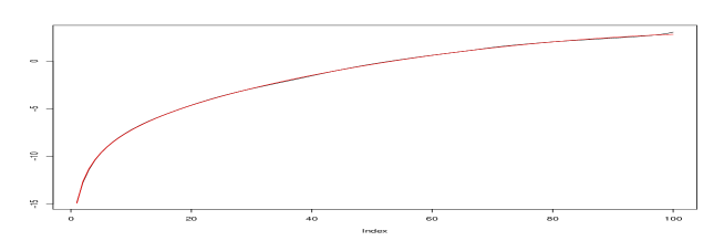
Figure 2: Top panel: The ordered values of the bottom panel of Figure 1. Centre panel: the means of the ordered values of 500 simulated samples. Bottom panel: the parametric approximation $f_{n,r,\sigma}(t)$ to the centre panel in red.

The order statistics of the process $N(t)$ can be approximated by $\exp(f_{n,r,\sigma}(t))$. Given $\varphi$ the order statistics of $Y(t)=\text{rpois}(\phi N(t))$ for a sample of size $n$ may be approximated by the function $\varphi\exp(f_{n,r,\sigma})$. As the $Y(t)$ are integers and the measure of approximation to be used is the Kolmogorov metric the values of $\varphi\exp(f_{n,r,\sigma})$ are replaced by the nearest integer $\text{int}(\varphi\exp(f_{n,r,\sigma}))$.

The upper panel of Figure 3 shows the ordered sample of the upper panel of Figure 1 in black and the function $\text{int}(10\exp(f_{100,\exp(3.6),0.3}))$ in red. The lower panel shows the distribution functions. The Kolmogorov distance is 0.06.

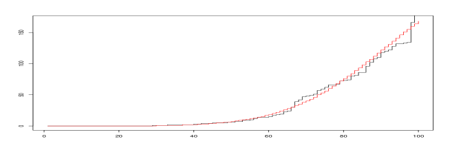
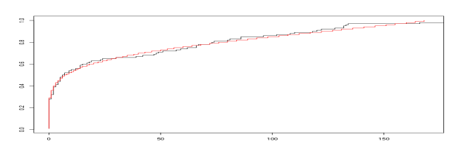
Figure 3: Upper panel: the order statistics of the first 100 values of the upper panel of Figure 1 in black and the parametric approximation $\text{int}(10\exp(f_{100,\exp(3.6),0.3}))$ in red. Lower panel: the distribution functions. The Kolmogorov distance is 0.06.

Based on 2000 simulations the 0.95-quantile of the Kolmogorov distance with for data generated with $\theta=(\exp(3.6),0.3,10)$ is 0.11. Thus not surprisingly the data of Figure 3 are consistent, in the sense of the Kolmogorov metric, with $\theta=(\exp(3.6),0.3,10)$ used to generate them.

The upper panel of Figure 4 shows a data of size $n=100$ generated with $\theta=(\exp(2.6),0.3,10)$. The lower panel shows its distribution function in black and that of $\text{int}(10\exp(f_{100,\exp(3.6),0.3}))$ in red. The Kolmogorov distance is 0.37 which far exceeds the 0.95-quantile of 0.11 for data generated with $\theta=(\exp(3.6),0.3,10)$. The conclusion is that the data are not consistent with the model $\theta=(\exp(3.6),0.3,10)$.

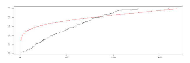
Figure 4: Upper panel: a sample of size $n=100$ generated with $\theta=(\exp(2.6),0.3,20)$. Lower panel: the distribution function of the data and that of the parametric approximation $\text{int}(10\exp(f_{100,\exp(3.6),0.3}))$ in red. The Kolmogorov distance is 0.44.

The above requires a value for $\varphi$ which may be obtained from the data as follows. Given the $N(t)$ the $Y(t)$ are defined by $Y(t)=\text{rpois}(\varphi N(t))$ so that

(9) $$\sum_{t=1}^{n}Y(t)\stackrel{{\scriptstyle D}}{{=}}\text{rpois}\Big{(}\varphi\sum_{t=1}^{n}N(t)\Big{)}.$$

Given $\beta$ a $\beta$-approximation interval for $\varphi\sum_{i=1}^{n}N(t)$ is given by $[\lambda_{l},\lambda_{u}]$ where

(10) $$\text{ppois}\Big{(}\sum_{t=1}^{n}Y(t),\lambda_{l}\Big{)}=(1+\beta)/2,\quad\text{ppois}\Big{(}\sum_{t=1}^{n}Y(t),\lambda_{u}\Big{)}=(1-\beta)/2.$$

which translates into the approximation interval

(11) $$\left[\,\frac{\lambda_{l}}{\sum_{t=1}^{n}N(t)},\frac{\lambda_{u}}{\sum_{t=1}^{n}N(t)}\,\right]$$

for $\varphi$.

A $\beta$-approximation interval for $\sum_{i=1}^{n}N(t)$ is given by the $(1-\beta)/2$ and $(1+\beta)/2$ quantiles $q_{l,N}(\beta)$ and $q_{u,N}(\beta)$ respectively. These can be obtained by simulations and saved together with the 20 parameter values required for $f_{n,r,\sigma}(t)$ giving 22 values in all. The default value of $\beta$ is $\beta=0.99$. The final approximation interval for $\varphi$ is

(12) $$\left[\,\frac{\lambda_{l}}{q_{u,N}(\beta)},\frac{\lambda_{u}}{q_{l,N}(\beta)}\,\right].$$

As an example for the data of Figure 1 we have $\sum_{t=1}^{n}Y(t)=3473$. For $\beta=0.99$ it follows from (10) that $\lambda_{l}=3323$ and $\lambda_{u}=3627$. For $(r,\sigma)=(\exp(3.6),0.3)$ simulations give $q_{l,N}(0.95)=342.0$ and $q_{u,N}(0.95)=378.2$. The final approximation region for $\varphi$ is $[3323/378.2,\,3627/342.0]=[8.79,\,10.61]$

Given such an interval a grid can be placed on it and the quantiles of the Kolmogorov metric obtained through simulations. These can be compared with the actual Kolmogorov distance of the data from $\text{int}(\varphi\exp(f_{n,r,\sigma}))$.

2.2 The dynamics of the process

The Kolmogorov distance depends only on the empirical distribution functions and takes no account of the dynamics of the process. This will be done by mimicking the dynamics of the $\log N(t)$ process by regressing $\log(y(t)/\varphi+\delta)$ on $\log(y(t-1)/\varphi+\delta)$ and $y(t-1)/\varphi$ for a choice of $\varphi$ and with default choice $\delta=0.01$.

The upper panel of Figure 5 shows a data set $Y(t)$ of size $n=100$ (black) generated with $\theta=(\exp(3.6),0.3,10)$ together with the forecast (red) ${\tilde{Y}}(t)$ of $Y(t)$ based on $Y(t-1)$;

(13) $${\tilde{Y}}(t)=\varphi\exp(\beta_{1}))(Y(t-1)/\varphi+\delta)^{\beta_{2}}\exp(\beta_{3}(Y(t-1)/\varphi+\delta))$$

where the $\beta_{j}$ with $\beta=(2.61,0.66,-0.82)$ are the regression coefficients. the lower panel does the same for the $N(t)$ process.

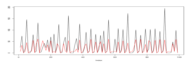
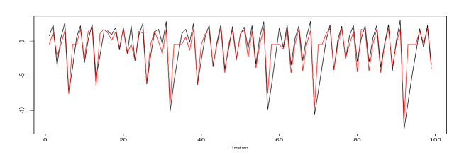
Figure 5: Upper panel: A data set generated with $\theta=(\exp(3.6),0.3,10)$ together with the forecast for $Y(t)$ based on $Y(t-1)$. Lower panel: the same for the $N(t)$ process.

The R output for the regression is

(14) $$\left\{\begin{array}[]{ccccc}&\text{Estimate}&\text{ Std. Error}&t&\text{value }Pr(>|t|)\\ \beta_{1}&2.60673&0.43069&6.052&2.76e-08***\\ \beta_{2}&0.66255&0.09178&7.219&1.23e-10***\\ \beta_{3}&-0.81973&0.06997&-11.716&<2e-16***\\ \end{array}\right.$$

with residual standard error: 2.381.

There are four statistics, the three values of the coefficients and the standard deviation of the residuals. Given a parameter $\theta$ simulations will give lower and upper bounds for these four values and these can be compared with the values obtained from the data at hand.

2.3 Accounting

Given a value of $\alpha$ in (3) the statistician has $1-\alpha$ of probability to spend. In all there are six statistics to be paid for: (i) the bounds for $\varphi$ as in (12), (ii) the Kolmogorov distance, (iii)-(v) bounds for the coefficients in the regression and (vi) for the standard deviation of the residuals.

The bounds for $\varphi$ differs in their construction from the others in using the lower and upper quantiles for $\sum_{t=1}^{100}N(t)$ in (12). The result is that the covering probability is almost one, much higher than the 0.98 would indicate. In a simulation study with 5000 simulations and $\theta=(\exp(3.6),0.3,10)$ the interval included the value of $\varphi=10$ in all but three of the the simulations, The actual cost of the interval for $\varphi$ is therefore very small and will be ignored.

Of the remaining five statistics the simplest choice is to spend an equal amount $(1-\alpha)/5$ on each, $\alpha_{j}=(4+\alpha)/5,j=1,\ldots,5,$ as in (5). In the case of the Kolmogorov distance it seems reasonable just to use the upper bound. This can also be argued for the standard deviation of the residuals but less convincingly. In all other cases lower and upper bounds are appropriate and treating these equally leave $(1-\alpha)/10$ to be spent on each.

As mentioned after (5) there may be some double counting so that the actual covering probability under the model may exceed the specified $\alpha$. In the extreme case the actual covering probability could be as high as $(4+\alpha)/5$ but it will generally be much lower than this. As an example for a $\alpha=0.9$ and $\theta=(\exp(3.6),0.3,10)$ 3000 simulations indicate a covering probability of approximately $\alpha^{*}=0.94$. If a more or less exact covering probability is required this can be obtained by replacing $\alpha=0.9$ by ${\tilde{\alpha}}=2\alpha-\alpha^{*}=0.86$. Simulations show that the covering probability is now close to 0.9 as required.

2.4 Approximating the data

Given a data set $y(t)$ of size $n$ and the function $f_{(n,r,\sigma)}$ an approximation interval $[\varphi_{l},\varphi_{u}]$ for $\varphi$ can be calculated derived as for (12). A grid size $m_{g}$ is placed over this interval which depends on the length of the interval. More precisely the gird size used is given by

$$ng=\max(10,(\varphi_{u}-\varphi_{l})/3)\,.$$

For the given $\alpha$ and $(r,\sigma)$ and a value of $\varphi$ on the grid simulations are run to calculate the relevant quantiles of the five statistics used. If all the relevant inequalities (4) are satisfied with ${\mbox{\boldmath$y$}}_{n}$ in place of ${\mbox{\boldmath$Y$}}_{n,\theta}$, then $P_{\theta}$ with $\theta=(r,\sigma,\varphi)$ is an adequate approximation to the data.

The output gives the bounds and the values for the data, the five $p$-values and the minimum $p$-value. For a simulated data of size $n=100$ with $\theta=(\exp(3.6),0.3,10)$ part of the output with $\alpha=0.86$ (see above) is given in (15).

(15) $$\left\{\begin{array}[]{ccc}(3.30,0.70,9.62),&(-0.12,2.16,2.38,0.10),&(0.57,1.00,1.05,0.14),\\ (-0.74,-0.57,-0.15,0.40),&(1.49,1.78,2.51,0.28),&(0.07,0.18,0.56).\\ \end{array}\right.$$

The first three numbers of (15 are the values of $\log r$, $\sigma$ and $\varphi$ in that order. The following four sets give, in order, the $(1-\alpha)/10$-quantile of the intercept term for the three regression coefficients and the residual standard deviation, followed by the value for the data $y(t)$ followed by the $(9+\alpha)/10$-quantile followed by the $p$-value. The last set of three numbers give the Kolmogorov distance for the data, the $(4+\alpha)/5$-quantile of the Kolmogorov distance and the $p$-value. The minimum $p$-value in (15) is 0.1.

A parameter $\theta=(r,\sigma,\varphi)$ is to be judged adequate if all the empirical values for the regression coefficients lie between the corresponding order statistics and the the Kolmogorov distance is less than the order statistic. This is the case for (15) and so $P_{\theta}$ with $\theta=(\exp(3.30),0.70,9.62)$ is judged to be an adequate approximation to the data.

For each value of the parameter $\theta=(r,\sigma,\varphi)$ the output gives 19 values which can be used to asses the degree of approximation. Likelihood gives only one. Figure 6 shows the minimum of the $p$-values plotted against the $r$, $\sigma$ and $\varphi$. This makes sense if all five statistics are treated equally. The largest minimum value is 0.494 attained for the parameter constellation $\theta=(\exp(3.716),0.315,10.97)$. The $\theta$ used to generate the data was $(\exp(3.6),0.3,10)$.

Figure 6: Top panel: the minimum $p$-value plotted against $r$. Centre panel: the minimum $p$-value plotted against $\sigma$. Bottom panel: the minimum $p$-value plotted against $\varphi$.

If $0.02$ probability is spent on each of the five statistics and if they were independent then the covering probability would be $0.98^{5}=0.904$, that is, very close to the $0.9$ used in the definition of the approximation region. In fact the four statistics deriving from the regression are highly correlated with the Kolmogorov distance being essentially independent of them. The correlation can be taken into account by calculating the covariance matrix and the Mahalanobis distances and then replacing the five $p$-values by the one based on these distances. Such a single $p$-value guarantees a correct covering probability. The plots corresponding to those of Figure 6 are shown in Figure 7 and are very disappointing. The smallest value of $r$ which is consistent with the data in the sense of the Mahalanobis distance is $\exp(1.18)$ with $\theta=(\exp(1.18),1.15,32.6)$ and a minimum $p$-value of 0.130.

The reason for this can be found by analysing the individual simulations. Most of the data sets of size $n=100$ generated with $\theta=(\exp(1.18),1.15,32.6)$ are so to speak unexceptional but the occasional one, 0.1%, may have as many as 97 zeros. That such data sets occur is due to the high value of $\sigma=1.15$. They results very high values for the regression coefficients and these in turn have a considerable influence on the covariance matrix which has a breakdown point of $1/n$.

Figure 7: Same as for Figure 6 but with $p$-values based on the Mahalanobis distances derived from the covariance matrix.

This last observation suggests using a covariance functional with a higher breakdown point. The one used here is due to John Kent and David Tyler and based on the multivariate $t$ distribution (see [Kent and Tyler, 1991]). If the $t$ distribution with $\nu$ degrees of freedom is used the breakdown point in $k$ dimensions is $1/(k+\nu)$ ([Dümbgen and Tyler, 2005]). For $\nu=2$ and $k=5$ it is 0.14. Figure 8 shows the resulting plots. They are an improvement on Figure 7 but still disappointing and much worse than Figure 6. It is not clear why this should be so. One possible reason is that the $p$-values leading to Figure 6 are based purely on quantiles and require no means or covariance matrices. This gives them a robustness not attainable from covariance functions. If one is only interested in the best approximation in some sense then attaining the exact covering probability $\alpha$ is not of high importance.

Figure 8: Same as for Figure 6 but with $p$-values based Mahalanobis distances derived from the Kent-Tyler covariance matrix with $\nu=2$.

The time required for analysing a data set of size $n=100$ is approximately 30 minutes using 3000 simulations and a grid $m_{g}=10$. If only 1000 simulations are used it reduces to about ten minutes. It is possible reduce this further by including a rough estimate of the number of zeros but this will not be discussed further.

2.5 Tables

The procedure described above requires values for $f_{n,r,\sigma}$. These can be obtained for a grid of values for $(r,\sigma)$ using simulations. The grid taken for the examples in the paper is given by

(16) $$r=1.05+4i/n_{g},\quad\sigma=0.05+1.1(i-1)/(n_{g}-1),\quad i=1,\ldots,n_{g}$$

with $n_{g}=30$. Clearly other choices are possible. The mean of the order statistics of $N(t)$ is obtained by simulations for each $(r,\sigma)$ in the grid. In this paper 10000 simulations were performed for each point $(r,\sigma)$ in the grid. The time required for the sample size $n=500$ was 35 minutes using Fortran 77 code. The simulations need only be performed once and can be stored for future use.

The top panel of Figure 9 shows data set of size 100 of $N(t)$ generated with $(r,\sigma)=(\exp(2.1),0)$, that is, a deterministic Ricker process. The centre panel shows the same but with $(r,\sigma)=(\exp(2.1),0.05)$. The bottom panel shows the expected values of the orders statistics of $N(t)$ again with $(r,\sigma)=(\exp(2.1),0.05)$.

Figure 9: Top panel: data set of size 100 of $N(t)$ with $(r,\sigma)=(\exp(2.1),0)$. Centre panel: data set of size 100 of $N(t)$ with $(r,\sigma)=(\exp(2.1),0.05)$. Bottom panel: expected values of the order statistics of $N(t)$ with $(r,\sigma)=(\exp(2.1),0.05)$.

The bottom panels shows that is is not a simple matter to obtain a good and yet parsimonious parametric approximation over the whole range. For this reason separate approximations were derived for the first $n/2$ order statistics and for those for $n/2+1$ to $n-2$. It proved difficult to approximate the two largest order statistics and so their values were simply included.

A linear regression was used with regressors

$$1,\,x,\,x^{2},\,x^{3},\,x^{4},\,x^{5},\,x^{6},\,\sin(3\pi x),\,\cos(3\pi x)$$

with $x=1:(n/2)$ for the first $n/2$ order statistics and $x=(n/2+1):(n-2)$ for the order statistics $n/2+1$ to $n-2$. The largest error over all the grid points was 3.08 for the order statistics $1:(n/2)$ and 0.37 for the order statistics $(n/2+1):(n-2)$. the 3.7 may seem large but the values of the order statistics where it occurs are -20 and less so the 3.08 hardly matter when the exponential is taken. It is possible that better results can be obtained by splines but this has not been attempted. The approximation requires storing 9+9+2=20 values for each pair $(r,\sigma)$. Two further values are required for the approximation interval for $\varphi$, namely the 0.005 and 0.995 quantiles of $\sum_{t=1}^{n}N(t)$, giving in all 22 values.

References

- [Buja et al., 2009] Buja, A., Cook, D., Hofmann, H., Lawrence, M., Lee, E.-K., Swayne, D., and Wickham, H. (2009). Statistical inference for exploratory data analysis and model diagnostics. Philosophical Transactions of the Royal Society A, 367:4361–4383.
- [Davies, 2014] Davies, L. (2014). Data Analysis and Approximate Models. Monographs on Statistics and Applied Probability 133. CRC Press.
- [Davies and Krämer, 2016] Davies, L. and Krämer, W. (2016). Stylized facts and simulating long range financial data. arXiv:1612.05229v1 [q-fin.ST].
- [Dümbgen and Tyler, 2005] Dümbgen, L. and Tyler, D. E. (2005). On the breakdown properties of some multivariate M-functionals. Scandinavian Journal of Statistics, 32:247–264.
- [Gutmann and Corander, 2015] Gutmann, M. U. and Corander, J. (2015). Bayesian optimization for likelihood-free inference of simulator-based statistical models. arXiv:1501.03291v3 [stat.ML].
- [Huber, 2011] Huber, P. J. (2011). Data Analysis. Wiley, New Jersey.
- [Kent and Tyler, 1991] Kent, J. T. and Tyler, D. E. (1991). Redescending M-estimates of multivariate location and scatter. Annals of Statistics, 19:2102–2119.
- [Neyman et al., 1953] Neyman, J., Scott, E. L., and Shane, C. D. (1953). On the spatial distribution of galaxies a specific model. Astrophysical Journal, 117:92–133.
- [Neyman et al., 1954] Neyman, J., Scott, E. L., and Shane, C. D. (1954). The index of clumpiness of the distribution of images of galaxies. Astrophysical Journal Supplement, 8:269–294.
- [Wood, 2010] Wood, S. N. (2010). Statistical inference for noisy nonlinear dynamic systems. Nature, 466(7310):1102–1104.