Evidence of a spectral break in the gamma-ray emission of the disk component of Large Magellanic Cloud: a hadronic origin?

Abstract

It has been suggested that high-energy gamma-ray emission ($>100{\rm\ MeV}$) of nearby star-forming galaxies may be produced predominantly by cosmic rays colliding with the interstellar medium through neutral pion decay. The pion-decay mechanism predicts a unique spectral signature in the gamma-ray spectrum, characterized by a fast rising spectrum (in $E^{2}F(E)$ representation) and a spectral break below a few hundreds of MeV. We here report the evidence of a spectral break around 500 MeV in the disk emission of Large Magellanic Cloud (LMC), which is found in the analysis of the gamma-ray data extending down to 60 MeV observed by Fermi-Large Area Telescope. The break is well consistent with the pion-decay model for the gamma-ray emission, although leptonic models, such as the electron bremsstrahlung emission, cannot be ruled out completely.

1 Introduction

It is generally believed that Galactic cosmic rays are accelerated by supernova remnant (SNR) shocks (Ginzburg & Syrovatskii, 1964). Cosmic-ray (CR) protons interact with the interstellar gas and produce neutral pions (schematically written as $p+p\rightarrow\pi^{0}+{\rm other\,products}$), which in turn decay into gamma rays. Cosmic-ray electrons can also produce gamma rays via bremsstrahlung and inverse Compton (IC) scattering emission (Strong et al., 2010; Chakraborty & Fields, 2013; Foreman et al., 2015). Detailed calculation of the CR propagation in our Galaxy using the GALPROP code finds that $\pi^{0}$-decay gamma rays form the dominant component of the diffuse Galactic emission (DGE) above 100 MeV, while the bremsstrahlung and IC emissions contribute a subdominant, but non-negligible fraction (Strong et al., 2010). GeV gamma-ray emissions have also been detected from nearby star-forming galaxies (Abdo et al., 2010a; Ackermann et al., 2012; Tang et al., 2014; Peng et al., 2016; Griffin et al., 2016), and they are interpreted as arising dominantly from cosmic-ray protons colliding with the interstellar gas as well (Pavlidou & Fields, 2002; Torres, 2004; Thompson et al., 2007; Stecker, 2007; Persic & Rephaeli, 2010; Lacki et al., 2011).

Although these theoretic arguments favor the pion-decay model for the GeV gamma-ray emission in these galaxies, there is no direct evidence for such pion-decay mechanism. Recently, Fermi- Large Area Telescope (hereafter LAT) detected a characteristic pion-decay feature in the gamma-ray spectrum of two supernova remnants, IC 443 and W44 (Ackermann et al., 2013). The pion-decay spectrum in the usual $E^{2}F(E)$ representation rises steeply below several hundred of MeV and then breaks to a softer spectrum. This characteristic spectral feature (often referred to as the “pion-decay bump”) uniquely identifies pion-decay gamma rays and thereby high-energy CR protons.

Motivated by this, we attempt to study the gamma-ray spectra of nearby star-forming galaxies and examine such unique pion-decay bump spectral signature. The LMC is the brightest external galaxies in gamma-ray emission, as it is very close to us (only 50 kpc). The LMC is near enough that individual star-forming regions can be resolved and thus their contribution can be removed so that one can obtain a relatively pure diffuse disk component. The high Galactic latitude of the LMC also leads to a low level of contamination due to the Galactic diffuse gamma-ray emission. We analyze the Fermi-LAT data of the LMC and pay special attention to the gamma-ray spectrum extending to 60 MeV using 8 years of Fermi-LAT Pass 8 data. We find that the gamma-ray spectrum shows a rise in $E^{2}F(E)$ representation at low-energies and breaks to a softer spectrum at about 500 MeV.

Our work is different from earlier works based on the Fermi-LAT observations of the LMC (Abdo et al., 2010b; Foreman et al., 2015; Ackermann et al., 2016), which focus on the gamma-ray emission above 200 MeV.

2 Data analysis and results

2.1 Data selection

The LAT Pass 8 data between 2008 August 4 and 2016 August 4 are taken from the Fermi Science Support Center (hereafter FSSC). Events with energy between 60 MeV and 100 GeV are selected. These data are analyzed using the Fermi Science Tools package (v10r0p5) available from the FSSC. We select “FRONT+BACK” SOURCE class events and use instrument response functions P8R2$\_$SOURCE$\_$V6. Events with zenith angles $>$90^∘ are excluded to reduce the contribution of Earth-limb gamma rays as well as that with the rocking angle of the satellite was larger than $52$ degrees. Gamma rays in a box Region Of Interest (ROI), 20${}^{\circ}\times$20^∘ centering at the position of RA.=80.894^∘, Dec=-69.756^∘, are used in the spectrum analysis between 60 MeV and 100 GeV, in which energy dispersion correction is considered. Binned maximum likelihood analysis are performed in this work.

2.2 Background sources

With a large angular containment of the low energy gamma-ray photons, all identified sources from the third LAT catalog (3FGL, Acero et al. (2015)) within 20^∘ from the center position are included. Four of them are excluded because they are located in the intensive LMC region (Ackermann et al., 2016), which correspond to 3FGL J0454.6-6825, 3FGL J0456.20-6924, 3FGL J0525.2-6614 and 3FGL J0535.3-6559. Another point source, 3FGL J0537.0-7113, is also at the edge of the LMC region and thus is excluded. These sources should be removed from the background sources so that the LMC sources can be distinguished significantly. A total of 72 point sources are included with fixed positions as in the 3FGL.

For sources within the ROI, the spectral parameters are fixed at the 3FGL catalog values except for their normalisations, which are allowed to be free. A total of 22 point sources are selected that allow the normalisations to be free, which are marked as black diamond in Fig. 1. For sources outside of ROI, all spectral parameters are fixed at the 3FGL catalog values.

The Galactic diffuse background and isotropic gamma-ray background are given by the templates “gll$\_$iem$\_$v06.fits” and “iso$\_$P8R2$\_$SOURCE$\_$V6$\_$v06.txt” available in the FSSC, while their normalizations are allowed to vary.

2.3 The LMC sources

2.3.1 The LMC point sources and extended sources

The LMC sources are categorized into two subparts, namely, the point ones and the extended ones.

We include four newly-identified point sources (namely P1, P2, P3, P4) in the LMC field in the analysis, which correspond to PSR J0540-6919, PSR J0537-6910/N157B, a gamma-ray binary CXOU J0536-6735 and N 132D respectively (Ackermann et al., 2016; Corbet et al., 2016). Their positions are determined by Ackermann et al. (2016).

Different templates are used for the extended sources found in the LMC field (Abdo et al., 2010b; Ackermann et al., 2016). Three spatial templates are considered and plotted in Fig. 2:

1. G template. Two-dimensional Gaussian template model for four sources (“G1”,“G2”,“G3”,“G4”), which is called the “analytic model” in Ackermann et al. (2016).

2. D template. A template model with the “Disk” and “30 Doradus” being modeled as a two-dimensional Gaussian. This template is used for the LMC in Abdo et al. (2010b) and is archived in the latest Fermi-LAT extended source template catalog.

3. H template. A gas model of the ionized Hydrogen employing the Southern H-Alpha Sky Survey Atlas intensity distribution (H_α) for the LMC diffusion region (Gaustad et al., 2001). The template is also used in the comparative analysis of gas models (Abdo et al., 2010b; Ackermann et al., 2016). We considered it because the gamma-ray emission of the LMC correlates better with ionized gas than that with other gases or the total gas (Abdo et al., 2010b; Ackermann et al., 2016), which might trace the population of young and massive stars.

2.3.2 Photon spectral models

The photon models of the LMC sources depend on the selection of energy bands. The first selection is to divide 0.06-100 GeV into 12 independent energy bands logarithmically ( i.e., performing spectral analysis on each independent energy band, hereafter the independent analysis). The second is to select a broad energy band (hereafter the broad-band analysis), which combine the several independent energy bands.

(1) For the independent analysis, we assume a single power law (PL) function to be the photon emission model of all LMC sources as used in Ackermann et al. (2013):

$$F(E)=K(E/E_{0})^{-\Gamma_{1}}$$ (1)

where $K$ is the normalisation, $E_{0}$ is the pivot energy of 200 MeV (hereafter all $E_{0}$ in other equations are fixed at 200 MeV) and $\Gamma_{1}$ is the power law index. For a narrow energy band in the independent analysis, $\Gamma_{1}$ is fixed at a common value of $2$ (Foreman et al., 2015).

(2) For the broad-band analysis, several photon emission models are employed. As discussed below, the broad-band analysis is performed for the template G only. Therefore we discuss the models for the G template. For the G1 component, we test the goodness of fit with two models, i.e., PL and Broken power law (BPL). The BPL model is given by:

$$F(E)=K(E/E_{0})^{-\Gamma_{1}}[1+(E/E_{\rm br})^{(\Gamma_{2}-\Gamma_{1})/s}]^{-s}$$ (2)

where $\Gamma_{1}$ and $\Gamma_{2}$ are the power law indices before and after the break energy $E_{\rm br}$, and $s$ is the smoothness of the break, which is fixed at $0.1$ (Ackermann et al., 2013).

For point source P1, its photon flux can be modeled with a PL with an exponential cutoff (PLC):

$$F(E)=K(E/E_{0})^{-\Gamma_{1}}\exp(-E/E_{c})$$ (3)

where $E_{c}$ is the exponential cutoff energy. Other extended sources (G2, G3, G4) and point sources (P2, P3, P4) are all modeled by a PL photon spectrum with photon index $\Gamma_{1}$ being free for the broad energy bands, which is different from the independent analysis of the narrow energy bands. Our model selection is consistent with that in Ackermann et al. (2016).

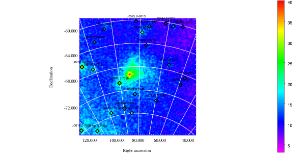
Figure 1: Gamma-ray count map of the $20^{\circ}\times 20^{\circ}$ fields around the LMC in the energy range from 60 MeV to 2.45 GeV observed by the Fermi-LAT. The nearby background point sources are marked with black diamonds. Events were spatially binned in pixels of side length $0.2^{\circ}$.

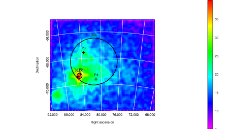
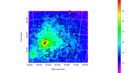
Figure 2: Locations of the LMC sources in the count map of the Fermi-LAT observation of 60 MeV to 2.45 GeV, in which the crosses of P1, P2, P3 and P4 are the LMC point sources while the circles or contour are the LMC extended sources. Top: G template, the diffusion region comprises four parts, each of which is assumed to be a two dimensional Gaussian profile (Ackermann et al., 2016); Center: D template, the LMC diffusion region makes use of the Disk and 30 Doradus, both of which employed the two dimensional Gaussian profile (Abdo et al., 2010b); Bottom: H template, a gas model of ionized Hydrogen employing the Southern H-Alpha Sky Survey Atlas intensity distribution for the LMC diffusion region (Gaustad et al., 2001).

2.4 Results

2.4.1 Results of the independent analysis

In the independent analysis, we divide the LAT gamma rays between 60 MeV and 100 GeV into 12 logarithmic spaced energy bands, in each of which the spectrum is fitted by a PL photon model with a fixed photon index of $2.0$.

The spectral results in three templates can be found in Fig. 3, in which both the extended and point sources are plotted. As a good residual count map is obtained and the value of “like2obj.getRetCode()” is zero, the fit thus is considered to be good in each independent band. The results of the large-scale disk in three templates can be found in Tab. 1. We discuss the results for each template following:

1. G template. The G template is useful to distinguish extended sources from point sources. Apparently, the 60 MeV-100 GeV spectrum of the G1 component cannot be fit by a PL function, thus we will test the fitting goodness with two functions, a PL and a BPL. Others three extended components can be fitted by a PL function within the uncertainties. The spectrum of the point source P1 decays rapidly up to $\sim$ 4 GeV, which could be fit by a PLC function. Other three point sources can be modeled with a PL function.

2. D template. The emission of the Disk component rises before several hundreds of  MeV and decays up to 100 GeV. The 30 Dor component is observed in eight independent energy bands, while in other 4 energy bands no significant emission is detected from the 30 Dor. It can be explained as that the luminous point sources P1 and P2 are lying near the center of the 30 Dor. The source P1 shows an initial fast decay and then exhibit no significant emission. The source P2 is observed in three higher energy independent bands ($>$ 5 GeV). The emission of the source P3 are detected in three lower energy bands ($<$ 5 GeV). The P4 source are decomposed in 6 energy bands, which can be fitted by a PL function.

3. H template. The emission of the H component rises quickly before 300 MeV followed by a flat spectrum behavior up to 1GeV, and then decays to 100 GeV. For the source P1, we obtained the low level emission in 2 independent energy bands. The source P3 and P4 can be significantly detected in four and six energy bands respectively, both of which show a PL decay. The emission of the source P2 is absent in this template. We found that, in the H template, the intensive region of the ionized Hydrogen is lying around the position of P1 and P2, which can account for the dim emission and non-detection of P1 and P2 respectively.

Table 1: Spectral data of the LMC large scale disk as well as the Galactic diffusion emission and the isotropic diffusion emission in the range of 60 MeV to 100 GeV measured by the Fermi-LAT.

Energy	Component	TS	$F_{Disk}$	$f_{Disk}$	$P_{g}$	$N_{i}$
MeV			$10^{-9}{\rm ph\ cm^{-2}\ s^{-1}}$	$10^{-11}{\rm erg\ cm^{-2}\ s^{-1}}$
60 - 111	G1	47	72.17 $\pm$ 24.12	0.93 $\pm$ 0.31	1.01 $\pm$ 0.04	1.16 $\pm$ 0.02
111 - 207	…	311	68.80 $\pm$ 13.90	1.64 $\pm$ 0.33	0.93 $\pm$ 0.03	1.17 $\pm$ 0.03
207 - 383	…	476	43.10 $\pm$ 4.23	1.91 $\pm$ 0.19	0.95 $\pm$ 0.02	1.14 $\pm$ 0.03
383 - 711	…	522	25.30 $\pm$ 1.51	2.08 $\pm$ 0.13	0.90 $\pm$ 0.01	1.27 $\pm$ 0.02
711 - 1320	…	481	14.20 $\pm$ 0.96	2.17 $\pm$ 0.15	0.94 $\pm$ 0.02	1.18 $\pm$ 0.07
1320 - 2449	…	199	5.54 $\pm$ 0.54	1.57 $\pm$ 0.15	0.95 $\pm$ 0.03	1.19 $\pm$ 0.11
2449 - 4545	…	126	2.74 $\pm$ 0.33	1.44 $\pm$ 0.17	0.89 $\pm$ 0.05	1.31 $\pm$ 0.15
4545 - 8434	…	52	1.19 $\pm$ 0.21	1.16 $\pm$ 0.21	0.93 $\pm$ 0.08	1.34 $\pm$ 0.15
8434 - 15651	…	7	0.29 $\pm$ 0.13	0.52 $\pm$ 0.24	1.31 $\pm$ 0.20	0.95 $\pm$ 0.17
15651 - 29042	…	22	0.32 $\pm$ 0.09	1.09 $\pm$ 0.31	0.89 $\pm$ 0.34	1.06 $\pm$ 0.21
29042 - 53891	…	$<1$	$<0.08$	$<0.73$	0.49 $\pm$ 0.71	1.34 $\pm$ 0.36
53891 - 100000	…	5	0.05 $\pm$ 0.03	0.63 $\pm$ 0.36	1.45 $\pm$ 1.02	0.92 $\pm$ 0.48
60 - 111	Disk	250	127.00 $\pm$ 27.30	1.64 $\pm$ 0.35	1.01 $\pm$ 0.04	1.16 $\pm$ 0.02
111 - 207	…	914	91.60 $\pm$ 5.41	2.19 $\pm$ 0.13	0.94 $\pm$ 0.03	1.17 $\pm$ 0.03
207 - 383	…	1229	51.30 $\pm$ 3.20	2.27 $\pm$ 0.14	0.96 $\pm$ 0.02	1.15 $\pm$ 0.03
383 - 711	…	1330	28.60 $\pm$ 1.35	2.36 $\pm$ 0.11	0.91 $\pm$ 0.02	1.32 $\pm$ 0.05
711 - 1320	…	985	14.00 $\pm$ 0.66	2.13 $\pm$ 0.10	0.94 $\pm$ 0.02	1.28 $\pm$ 0.08
1320 - 2449	…	524	6.06 $\pm$ 0.36	1.72 $\pm$ 0.10	0.96 $\pm$ 0.03	1.28 $\pm$ 0.12
2449 - 4545	…	297	2.86 $\pm$ 0.22	1.51 $\pm$ 0.12	0.90 $\pm$ 0.05	1.43 $\pm$ 0.16
4545 - 8434	…	191	1.47 $\pm$ 0.14	1.44 $\pm$ 0.14	0.93 $\pm$ 0.08	1.41 $\pm$ 0.15
8434 - 15651	…	48	0.48 $\pm$ 0.09	0.87 $\pm$ 0.16	1.31 $\pm$ 0.19	0.98 $\pm$ 0.16
15651 - 29042	…	55	0.35 $\pm$ 0.07	1.19 $\pm$ 0.22	0.90 $\pm$ 0.34	1.10 $\pm$ 0.21
29042 - 53891	…	10	0.09 $\pm$ 0.04	0.57 $\pm$ 0.23	0.48 $\pm$ 0.69	1.36 $\pm$ 0.34
53891 - 100000	…	6	0.05 $\pm$ 0.02	0.54 $\pm$ 0.28	1.44 $\pm$ 1.04	0.97 $\pm$ 0.48
60 - 111	H	421	174.00 $\pm$ 30.10	2.24 $\pm$ 0.39	1.01 $\pm$ 0.04	1.16 $\pm$ 0.02
111 - 207	…	2080	140.00 $\pm$ 13.60	3.35 $\pm$ 0.33	0.94 $\pm$ 0.03	1.17 $\pm$ 0.03
207 - 383	…	2600	75.00 $\pm$ 3.08	3.33 $\pm$ 0.14	0.96 $\pm$ 0.02	1.14 $\pm$ 0.03
383 - 711	…	2928	41.20 $\pm$ 1.23	3.39 $\pm$ 0.10	0.91 $\pm$ 0.02	1.29 $\pm$ 0.05
711 - 1320	…	2587	21.00 $\pm$ 0.65	3.20 $\pm$ 0.10	0.94 $\pm$ 0.02	1.23 $\pm$ 0.08
1320 - 2449	…	1071	8.34 $\pm$ 0.44	2.37 $\pm$ 0.13	0.96 $\pm$ 0.03	1.27 $\pm$ 0.12
2449 - 4545	…	480	3.52 $\pm$ 0.25	1.85 $\pm$ 0.13	0.89 $\pm$ 0.05	1.45 $\pm$ 0.16
4545 - 8434	…	398	1.82 $\pm$ 0.15	1.77 $\pm$ 0.15	0.93 $\pm$ 0.08	1.42 $\pm$ 0.15
8434 - 15651	…	106	0.61 $\pm$ 0.09	1.11 $\pm$ 0.17	1.30 $\pm$ 0.18	0.98 $\pm$ 0.16
15651 - 29042	…	53	0.33 $\pm$ 0.07	1.10 $\pm$ 0.23	0.85 $\pm$ 0.35	1.17 $\pm$ 0.21
29042 - 53891	…	24	0.14 $\pm$ 0.04	0.88 $\pm$ 0.27	0.49 $\pm$ 0.68	1.33 $\pm$ 0.34
53891 - 100000	…	2	0.03 $\pm$ 0.03	0.31 $\pm$ 0.30	1.35 $\pm$ 1.05	1.08 $\pm$ 0.49

Among the three templates, the G template is the best one to decompose the LMC extended and point sources in the independent energy bands. In order to obtain the spectrum of a pure large-scale disk component (G1), we perform an analysis using the G template in the sections below.

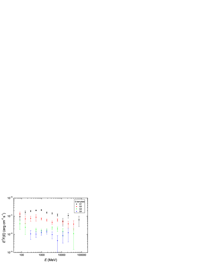
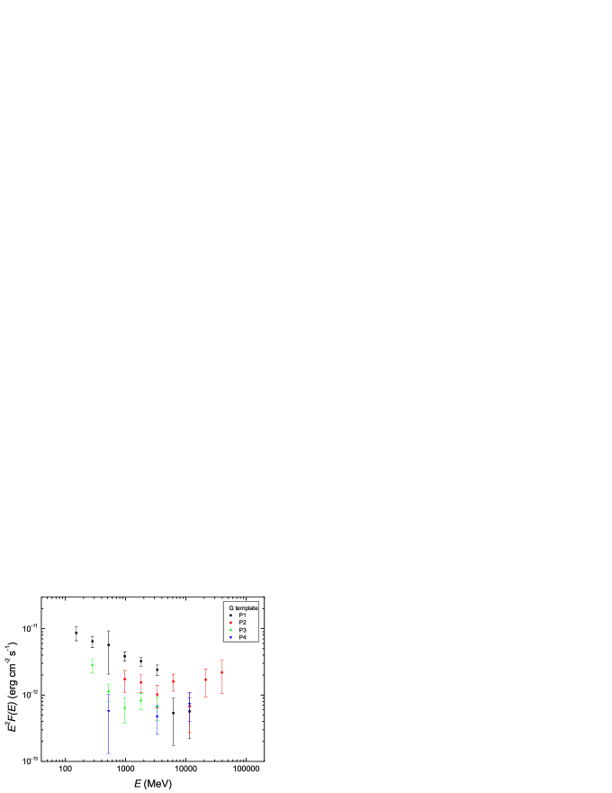
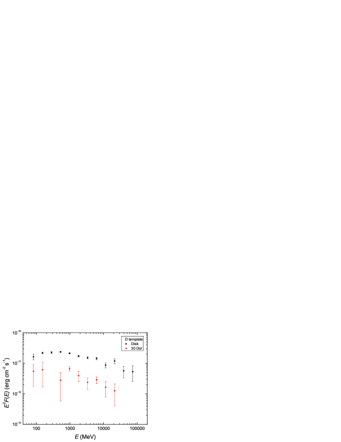
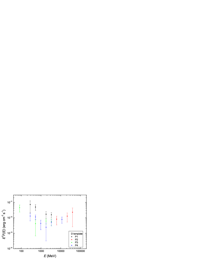
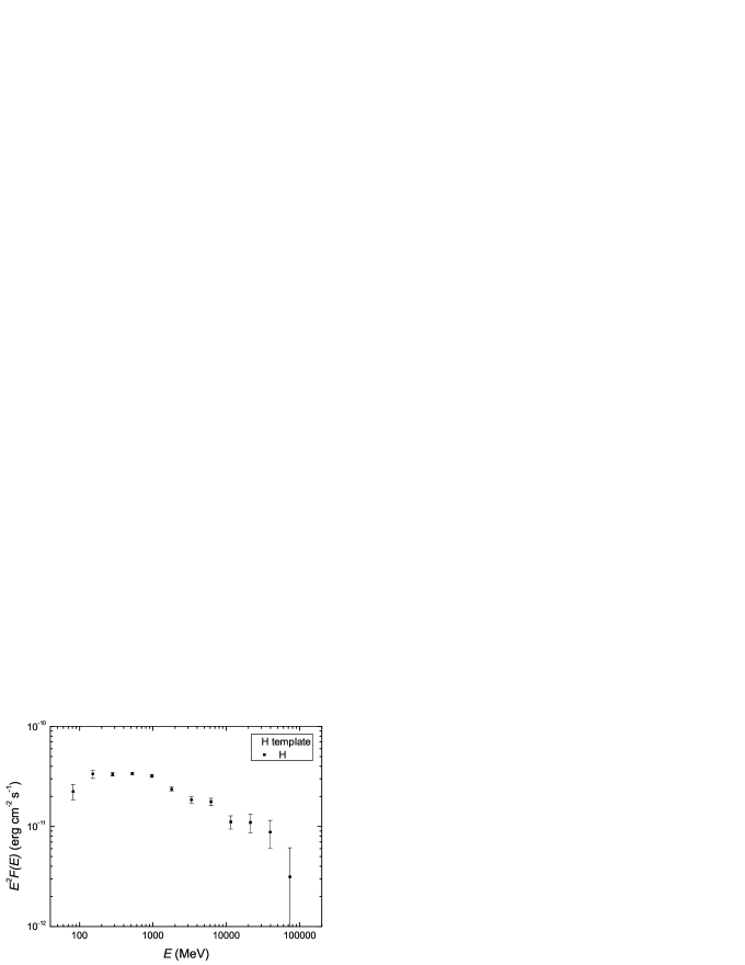
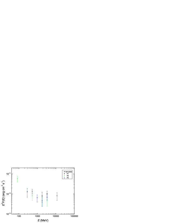
Figure 3: The gamma-ray spectral data of the LMC extended components and point sources by the independent analysis. Top for the G template, middle for the D template and bottom for the H template. In order to be visible of the spectrum behavior, the upper limits are not plotted.

2.4.2 Results of the broad-band analysis

As shown in Fig. 3, the spectrum of the independent analysis in the G template has a rapid rise below about 500 MeV and then transits to a much softer spectrum. To quantify the significance of the spectral break, we perform comparative fitting in two broad-band energy ranges, i.e., 0.06-2.45 GeV and 0.06-100 GeV. The former energy range covers the 6 independent energy bands and is close to the energy range (0.06-2 GeV) used in Ackermann et al. (2013), in which a characteristic $\pi^{0}$ decay feature is reported to be found in two Galactic SNRs. The latter energy range is selected in order to test whether the BPL is still a good function to fit the gamma-ray emission up to 100 GeV.

Given an input photon model, the probability of obtaining the data as observed is noted by $L$, which is the product of the probabilities of obtaining the observed counts by the LAT in each bin, i.e.,

$$L=\prod_{k}\frac{m_{k}^{n_{k}}e^{-m_{k}}}{n_{k}!}=e^{-N_{pred}}\prod_{k}\frac{m_{k}^{n_{k}}}{n_{k}!}$$ (4)

where $k$ is an index over image pixels in both space and energy, $m_{k}$ indicates the number of counts predicted by the model at pixel $k$, $n_{k}$ is the observed number of counts at pixel $k$, and $N_{pred}$ is the total number of observed counts .

We calculate the test-statistic value (TS) defined as $-2\log(L_{0}/L_{1})$, where $L_{0},L_{1}$ correspond to the likelihood value for the case without the G1 component, with the G1 component respectively (Mattox et al., 1996). Since the BPL is a nested model with two additional degrees of freedom (dof) more than the PL, a significant change can be reached when ${\rm\Delta TS}$ is larger than 25 ($\sim 5\sigma$) from the BPL to the PL, where ${\rm\Delta TS}$ approximately follows the $\chi^{2}$ distribution (Ackermann et al., 2013; Harris et al., 2014).

First, we fit the spectrum between 0.06 GeV and 2.45 GeV with the PL and the BPL functions. The BPL yields a significantly larger TS value than the PL, with an improvement of $\Delta{\rm TS}=66$ (see Tab. 2), i.e., statistical significance of $\sim 8.1\sigma$. The photon index is $\Gamma_{1}=1.48\pm 0.09$ below the break energy of $497\pm 78$ MeV, above which the photon index is $\Gamma_{2}=2.35\pm 0.11$. Second, we test if the BPL model can fit the data in a border energy range, i.e., 0.06-100 GeV. The BPL still yields a larger TS value, with an improvement of $\Delta{\rm TS}=180$, i.e., statistical significance of $\sim 13.4\sigma$ over the PL. The photon index is $\Gamma_{1}=1.39\pm 0.03$ below the break energy of $532\pm 20$ MeV, above which the photon index is $\Gamma_{2}=2.40\pm 0.03$. The results in both two broad energy bands show that the BPL is the better function to fit the gamma rays of the G1 component, indicating that a break at $\sim$500 MeV exists in the spectrum of the large scale disk component of the LMC.

2.4.3 Comparative analysis without the data between 60-200 MeV

To compare with the results in the former literature (Ackermann et al., 2016), we perform the spectrum analysis on the Fermi-LAT data after removing the data of 60-200 MeV, i.e., in the energy range of 0.2-2.45 GeV and 0.2-100 GeV. The results are shown in Tab. 2. In the former energy range, the PL fitting gives an photon index of about $2.0$, which is softer than that includes the data below 200 MeV. The BPL has an improvement of $\Delta{\rm TS}=32$ to the PL, i.e., statistical significance of $\sim 5.7\sigma$. This, however, is lower than the improvement in the case including the data in 60-200 MeV, that is $\sim 8.1\sigma$.

In case of 0.2-100 GeV, the BPL with a break energy of $490\pm 18$ MeV is found to give a better fit than the PL. However, the change in TS of 70, say $\sim 8.4\sigma$, is much smaller than the case including the data in 60-200 MeV, that is $\sim 13.4\sigma$.

The significant improvement of the fit when including the low energy data of 60-200 MeV favors the existence of the $\pi^{0}$ decay bump in the gamma-ray spectrum of the LMC disk. The 60-200 MeV data also provide extra flux points to constrain the physical model parameters statistically, see Sec. 4.

Table 2: Broad-band analysis results of the G1 component.

Model	E	Component	K	$\Gamma_{1}$	$\Gamma_{2}$	$E_{\rm br}$	$\log L_{0}$	$\log L_{1}$	${\rm TS}$	$\Delta{\rm TS}$
	GeV					MeV
PL	0.06-2.45	G1	$4.0\pm 0.2$	$1.89\pm 0.03$	-	-	-546725	-546350	750	-
BPL	…	…	$3.8\pm 0.1$	$1.48\pm 0.09$	$2.35\pm 0.11$	$497\pm 78$	…	-546317	816	66
…
PL	0.06-100	…	$4.1\pm 0.2$	$2.06\pm 0.02$	-	-	-261700	-261305	790	-
BPL	…	…	$3.4\pm 0.1$	$1.39\pm 0.03$	$2.40\pm 0.03$	$532\pm 20$	…	-261215	970	180
PL	0.2-2.45	G1	$4.8\pm 0.3$	$2.01\pm 0.04$	-	-	-418860	-418499	722	-
BPL	…	…	$3.3\pm 0.1$	$1.21\pm 0.03$	$2.27\pm 0.03$	$429\pm 10$	…	-418483	754	32
…
PL	0.2-100	…	$5.2\pm 0.2$	$2.15\pm 0.02$	-	-	-264997	-264589	816	-
BPL	…	…	$3.0\pm 0.1$	$1.21\pm 0.04$	$2.34\pm 0.03$	$490\pm 18$	…	-264554	886	70

3 The physical models

In this section, we explore the origin of the diffuse gamma-ray emission by the physical models. We consider two radiation models for the gamma-ray data between 60 MeV and 100 GeV, i.e., the electron bremsstrahlung model and the neutral pion decay model.

3.1 The electron bremsstrahlung model

In the electron bremsstrahlung model, we consider both a PL distribution $dN_{e}/dE_{e}\propto E_{e}^{-s_{e1}}$ and a BPL distribution, i.e., $dN_{e}/dE_{e}=C_{e}(E_{e}/E_{b,e})^{-s_{e1}}$ and $dN_{e}/dE_{e}=C_{e}(E_{e}/E_{b,e})^{-s_{e2}}$ below and above the break energy $E_{b,e}$, for the injected electrons. The bremsstrahlung emission flux emitted by ultra-relativistic electrons can then be given by Stecker (1971) and Foreman et al. (2015):

$$E_{\gamma}^{2}F_{brem}(E_{\gamma})=E_{\gamma}\int_{E_{\gamma}}^{E_{max}}cn_{H}\sigma_{brem}b^{-1}(E_{e})N_{e}(E_{e})dE_{e}$$ (5)

where $\sigma_{brem}=\frac{4\alpha}{\pi}\sigma_{\rm T}\ln(183)\simeq 3.22\times 10^{-26}\rm\ cm^{2}$ is the cross section, in which $\alpha$ is fine structure constant, and $\sigma_{\rm T}$ is the Thomson scattering cross section, see Equation (23) of Foreman et al. (2015). $c$ is the speed of light and $E_{max}$ is fixed to 2 TeV in the calculation, which results in a rollover at high energies, improving the agreement with the GALPROP model beyond 100 GeV (Strong et al., 2011; Chakraborty & Fields, 2013). Here $b(E_{e})$ is the sum of electron energy-loss rates by synchrotron radiation, inverse-Compton scattering, bremsstrahlung radiation and ionization (Ginzburg & Syrovatskii, 1964; Foreman et al., 2015), i.e.,

$$b(E_{e})=b_{syn}(E_{e})+b_{IC}(E_{e})+b_{brem}(E_{e})+b_{ion}(E_{e}).$$ (6)

where $b_{syn}\varpropto B^{2}$ ($B$, magnetic field intensity in unit of ${\rm\mu G}$), $b_{IC}\varpropto{\rm U_{ph}}$ (${\rm U_{ph}}$, photon energy density in unit of ${\rm eVcm^{-3}}$), $b_{brem}\varpropto n_{\rm H}$ and $b_{ion}\varpropto n_{\rm H}$ ($n_{\rm H}$, the density of hydrogen atom in unit of ${\rm\ cm^{-3}}$), see Equation (32) to (37) of Foreman et al. (2015). There are five free parameters for bremsstrahlung model with a PL injection electron distribution, i.e., $n_{\rm H}$, $B$, ${\rm U_{ph}}$, the normalisation (${\rm C}_{e}$) and the injected electron spectrum index ($s_{e1}$). As for a BPL electron distribution, two additional free parameters are considered, i.e., the post-break spectrum index ($s_{e2}$) and the break energy ($E_{b,e}$).

3.2 The neutral pion decay model

For the neutral pion decay model, the gamma-ray flux is calculated by the semi–analytical method proposed by Kelner et al. (2006):

$$E_{\gamma}^{2}F_{\pi}(E_{\gamma})=E_{\gamma}^{2}\int_{E_{\gamma}}^{\infty}cn_{H}{\sigma}_{pp}(E_{p})\frac{dN_{p}}{dE_{p}}(E_{p})f_{\gamma}(\frac{E_{\gamma}}{E_{p}},E_{p})\frac{dE_{p}}{E_{p}}$$ (7)

where $\sigma_{pp}=10^{-27}(34.3+1.88M+0.25M^{2})(1-(1.22{\rm TeV}/E_{p})^{4})^{2}\rm\ cm^{2}$ is the cross section of proton-proton collision, in which $M=\ln(E_{p}/{\rm 1TeV})$, see Equation (79) of Kelner et al. (2006). Here $dN_{p}/dE_{p}=C_{p}E_{p}^{-s_{p}}$ is the spectrum of cosmic-ray protons with $C_{p}$ a normalisation, and $f_{\gamma}$ is the spectrum of secondary gamma rays produced in a single proton-proton collision, with $E_{p}$ and $E_{\gamma}$ being the cosmic-ray proton energy and the generated gamma-ray energy respectively. There are two free parameters in this model: the proton index $s_{p}$ and the product (defined as $C^{\ \prime}_{p}$) of the normalization of the proton spectrum $C_{p}$ and the density of hydrogen atoms $n_{\rm H}$, since the $n_{\rm H}$ can be extracted from the integration.

4 Modeling Result and Discussion

4.1 Method

For our fitting of 11 flux points, the $\chi^{2}$ can be derived:

$$\chi^{2}=\sum_{i=1}^{11}{\frac{(f_{m,i}-f_{obs,i})^{2}}{\sigma_{f_{obs,i}}^{2}}}$$ (8)

where $f_{m,i}$ is the predicted flux by the physical model, $f_{obs,i}$ is the LAT-observed flux ($E^{2}F(E)$) in the the $i$th energy bin with corresponding error of $\sigma_{f_{obs,i}}$. A $\chi^{2}$ comparable with the degrees of freedom (dof) is considered as an acceptable fit, i.e., the reduced $\chi^{2}$ (labeled as $\chi_{r}^{2}$) is between 0.75 and 1.50 (Zhang et al., 2011). After deriving a best fit, the resultant $\chi^{2}$ is labeled as $\chi^{2}_{\rm best}$. The $1\sigma$ error of a parameter is calculated by $\chi^{2}_{\rm error}=\chi^{2}_{\rm best}+\chi^{2}_{1\sigma}$ while other parameters are fixed at the best-fit values. $\chi^{2}_{1\sigma}$ can be calculated by integrating the $\chi^{2}$ probability density function of the corresponding degrees of freedom to 1$\sigma$.

In our following analysis, we also consider that if the resultant parameter values are consistent with values from other papers or observations (hereafter reference values). For example, when Bremsstrahlung losses dominates the gamma-ray emission, $n_{\rm H}$ can be high as $2{\rm\ cm^{-3}}$ (Kim et al., 2003). The inverse Compton losses are not important and thus we consider a low photon energy density of ${\rm U_{ph}=0.57\ eVcm^{-3}}$ (Israel et al., 2010), where we also set a lower boundary of ${\rm U_{ph,limit}=0.01\ eVcm^{-3}}$. For the magnetic field strength, $B$ could be in the range of ${\rm 2-7\ \mu G}$ (Gaensler et al., 2005; Abdo et al., 2010b; Mao et al., 2012; Foreman et al., 2015).

4.2 Modeling Results

Bremsstrahlung with the PL injected electron spectrum. First, all parameters are unfixed. The results can be found in Tab. 3. This fit is acceptable with $\chi_{r}^{2}=1.28$. However, the resultant electron spectrum index of $1.39_{+0.12}^{-0.11}$ is much harder than that in our Galaxy, i.e., $2.0-2.4$ (Porter & Protheroe, 1997). Then we allow the electron spectrum index to vary between $2.0-2.4$ and find that smaller values of the electron spectrum index will result in smaller $\chi_{r}^{2}$ close to $1$, which means a good fit. Fixing the electron spectrum index of $2.0$, it leads to a bit worse goodness of $\chi_{r}^{2}=1.70$, but gives the constrains on all parameters, i.e., $n_{\rm H}=1.14_{+0.10}^{-0.10}\ {\rm\ cm^{-3}}$, $B=4.94_{+0.34}^{-0.31}\ {\rm\mu G}$, ${\rm U_{ph}}=0.81_{+1.18}^{-0.62}\ {\rm eVcm^{-3}}$, which are comparable to the reference values. The fit with fixed electron spectral index is considered and plotted in Fig. 4.

Bremsstrahlung with the BPL injected electron spectrum. Initially all parameters are allowed to float. The photon energy density is attacking the lower boundary in this fitting. Thus we fixed it at 0.01 and fit the data again. The fit is good to constrain all parameters and $\chi_{r}^{2}=1.33$. We note that the magnetic field strength ($B$) of $\sim 0.08{\rm\ \mu G}$ is much lower than the reference value, i.e, $2-7{\rm\mu G}$ as discussed above. In addition, we use the same electron spectrum as that in our Galaxy, which is also used for the LMC in Foreman et al. (2015), i.e., $s_{e1}=1.80,s_{e1}=2.25$ and $E_{b,e}=4$ GeV. This fit is a bit worse, i.e., $\chi_{r}^{2}=2.04$. The derived parameters, i.e., $n_{\rm H}=1.43_{+0.14}^{-0.13}\ {\rm\ cm^{-3}}$, $B=4.84_{+0.35}^{-0.30}\ {\rm\mu G}$, ${\rm U_{ph}}=0.60_{+1.34}^{-0.69}\ {\rm eVcm^{-3}}$, are comparable to the reference values. Thus the fit with same electron spectrum distribution as that of our Galaxy is adopted and plotted in Fig. 4.

In the pion decay model, the resultant value of chi-square, i.e., $\chi_{r}^{2}=0.85$, implies a reasonable fit to the data. The best-fit value of the proton index ($s_{p}$) is $2.45_{+0.14}^{-0.13}$, which is consistent with the proton index (2.4) obtained by Foreman et al. (2015). Fig. 4 shows the result of the pion decay model. Without fixing other parameters, the pion decay model thus is a preferred model to model the gamma-ray emission from the G1 component with an accepted $\chi_{r}^{2}$ value.

Table 3: Derived parameters from the physical models for the G1 component.

Model	${n_{\rm H}}$	$B$	${\rm U_{ph}}$	$s_{e1}$	$s_{e2}$	$E_{e,b}$	$s_{p}$	$\chi^{2}/$dof	$\chi_{r}^{2}$
	${\rm cm^{-3}}$	${\mu G}$	${\rm eVcm^{-3}}$			MeV
Bremsstrahlung	$0.39_{+0.03}^{-0.03}$	$2.99_{+0.20}^{-0.17}$	$7.80_{+6.73}^{-3.15}$	$1.39_{+0.12}^{-0.11}$	-	-	-	7.7/6	1.28
…	$1.14_{+0.10}^{-0.10}$	$4.94_{+0.34}^{-0.31}$	$0.81_{+1.18}^{-0.62}$	2.00(fixed)	-	-	-	11.9/7	1.70
Bremsstrahlung with Break	$2.59_{+0.19}^{-0.19}$	$0.08_{+0.004}^{-0.003}$	0.01(fixed)	$1.45_{+0.42}^{-0.74}$	$2.41_{+0.06}^{-0.06}$	$1318_{+442}^{-382}$	-	6.7/5	1.33
…	$1.43_{+0.14}^{-0.13}$	$4.84_{+0.35}^{-0.30}$	$0.60_{+1.34}^{-0.69}$	1.80(fixed)	2.25(fixed)	4000(fixed)	-	14.3/7	2.04
$\pi^{0}$ decay	-	-	-	-	-	-	$2.45_{+0.14}^{-0.13}$	7.6/9	0.85

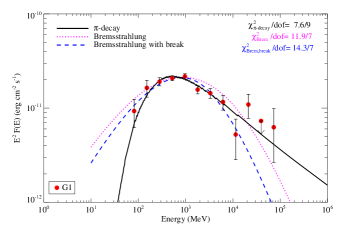
Figure 4: Physical modeling of the G1 component. The red points are the energy fluxes of the G1 component measured by the Fermi-LAT, in which the errors are statistical only and the upper limit is at 95% confidence level. The solid line is the modeling result of the neutral pion decay. The dotted line is for the Bremsstrahlung model with a PL electron spectrum, whose power index is fixed at $2.0$. The dashed line is for the Bremsstrahlung model with a BPL electron spectrum, whose distribution is same as that of our Galaxy but with a parameterized normalisation (Foreman et al., 2015). The derived parameter values of these models are present in Tab. 3.

5 Discussion and Conclusion

Abdo et al. (2010a) first notice that the gamma-ray emission of the LMC, as detected by the Fermi-LAT, is likely diffuse, i.e., it consists of two diffusion regions, Disk and 30 Doradus. Foreman et al. (2015) re-analyze the data by employing several combinations of the ionizing gas (H_α) and 160$\mu m$ radiation. They find that the leptonic processes also contribute to the gamma-ray emission of the LMC, i.e., about 3% of the Disk (excluding 30 Doradus) gamma-ray flux is from inverse Compton and 18% is from Bremsstrahlung. Employing the high energy photons above 200 MeV with 6 flux points, they find a proton spectrum index of $2.4$.

After subtracting the bright LMC point sources detected by Fermi-LAT (Fermi LAT Collaboration et al., 2015), four diffusion components are decomposed from the LMC region in an emissivity template (Ackermann et al., 2016). In this template, they suggest the different origins for these four decomposed diffusion components, i.e., E0, E2, E4 and E1+E3. The emissions from the large-scale disk (E0 component, largely overlapping with the G1), is likely dominated by hadronic process while others are likely of leptonic origins. For example, the E2 (largely overlapping with the G3) and the E4 (largely overlapping with the G4) could originate from the inverse-Compton process. The E1+E3 component (largely overlapping with the G2) is more favorable for the leptonic origin. Without considering the data below 200 MeV, the spectrum of the E0 is not visible of the $\pi^{0}$ decay feature.

In this work, we analyzed the high-energy gamma-ray spectra of the large-scale disk in the LMC, including the data between 60-200 MeV that was not considered in previous works. We decomposed a large-scale disk, i.e., the G1 component, from other spatial components in the LMC, and, for the first time, found a spectrum break around 500 MeV for the disk. The obtained gamma-ray emission can be well reproduced by the pionic gamma rays from $pp-$collision between the gas in the LMC disk and protons with a bit harder spectrum than that in our Galaxy, while the bremsstrahlung emission is marginally consistent with the observed spectrum. We conclude that, the current Fermi-LAT data of the LMC large scale disk emission favors a hadronic origin, although a leptonic model cannot be ruled out completely.

References

- Abdo et al. (2010a) Abdo, A. A., Ackermann, M., Ajello, M., et al. 2010a, ApJ, 709, L152
- Abdo et al. (2010b) Abdo, A. A., Ackermann, M., Ajello, M., et al. 2010b, A&A, 512, A7
- Acero et al. (2015) Acero, F., Ackermann, M., Ajello, M., et al. 2015, ApJS, 218, 23
- Acero et al. (2016) Acero, F., Ackermann, M., Ajello, M., et al. 2016, ApJS, 223, 26
- Ackermann et al. (2012) Ackermann, M., Ajello, M., Allafort, A., et al. 2012, ApJ, 755, 164
- Ackermann et al. (2013) Ackermann, M., Ajello, M., Allafort, A., et al. 2013, Science, 339, 807
- Ackermann et al. (2016) Ackermann, M., Albert, A., Atwood, W. B., et al. 2016, A&A, 586, A71
- Chakraborty & Fields (2013) Chakraborty, N., & Fields, B. D. 2013, ApJ, 773, 104
- Corbet et al. (2016) Corbet, R., Chomiuk, L., Coe, M., et al. 2016, ApJ, 829, 105
- Fermi LAT Collaboration et al. (2015) Fermi LAT Collaboration, Ackermann, M., Albert, A., et al. 2015, Science, 350, 801
- Foreman et al. (2015) Foreman, G., Chu, Y.-H., Gruendl, R., et al. 2015, ApJ, 808, 44
- Gaensler et al. (2005) Gaensler, B. M., Haverkorn, M., Staveley-Smith, L., et al. 2005, Science, 307, 1610
- Gaustad et al. (2001) Gaustad, J. E., McCullough, P. R., Rosing, W., & Van Buren, D. 2001, PASP, 113, 1326
- Ginzburg & Syrovatskii (1964) Ginzburg, V. L., & Syrovatskii, S. I. 1964, The Origin of Cosmic-Ray, New York: Macmillan, 1964
- Griffin et al. (2016) Griffin, R. D., Dai, X., & Thompson, T. A. 2016, ApJ, 823, L17
- Harris et al. (2014) Harris, J., Chadwick, P. M., & Daniel, M. K. 2014, MNRAS, 441, 3591
- Israel et al. (2010) Israel, F. P., Wall, W. F., Raban, D., et al. 2010, A&A, 519, A67
- Kelner et al. (2006) Kelner, S. R., Aharonian, F. A., & Bugayov, V. V. 2006, Phys. Rev. D, 74, 034018
- Kim et al. (2003) Kim, S., Staveley-Smith, L., Dopita, M. A., et al. 2003, ApJS, 148, 473
- Lacki et al. (2011) Lacki, B. C., Thompson, T. A., Quataert, E., Loeb, A., & Waxman, E. 2011, ApJ, 734, 107
- Mao et al. (2012) Mao, S. A., McClure-Griffiths, N. M., Gaensler, B. M., et al. 2012, ApJ, 759, 25
- Mattox et al. (1996) Mattox, J. R., Bertsch, D. L., Chiang, J., et al. 1996, ApJ, 461, 396
- Peng et al. (2016) Peng, F.-K., Wang, X.-Y., Liu, R.-Y., Tang, Q.-W., & Wang, J.-F. 2016, ApJ, 821, L20
- Pavlidou & Fields (2002) Pavlidou, V., & Fields, B. D. 2002, ApJ, 575, L5
- Persic & Rephaeli (2010) Persic, M., & Rephaeli, Y. 2010, MNRAS, 403, 1569
- Porter & Protheroe (1997) Porter, T. A., & Protheroe, R. J. 1997, Journal of Physics G Nuclear Physics, 23, 1765
- Stecker (1971) Stecker, F. W. 1971, NASA Special Publication, 249
- Stecker (2007) Stecker, F. W. 2007, Astroparticle Physics, 26, 398
- Strong et al. (2010) Strong, A. W., Porter, T. A., Digel, S. W., et al. 2010, ApJ, 722, L58
- Strong et al. (2011) Strong, A. W., Orlando, E., & Jaffe, T. R. 2011, A&A, 534, A54
- Tang et al. (2014) Tang, Q.-W., Wang, X.-Y., & Tam, P.-H. T. 2014, ApJ, 794, 26
- Thompson et al. (2007) Thompson, T. A., Quataert, E., & Waxman, E. 2007, ApJ, 654, 219
- Torres (2004) Torres, D. F. 2004, ApJ, 617, 966
- Zhang et al. (2011) Zhang, B.-B., Zhang, B., Liang, E.-W., et al. 2011, ApJ, 730, 141