On time and consistency in multi-level agent-based simulations

Abstract

The integration of multiple viewpoints became an increasingly popular approach to deal with agent-based simulations. Despite their disparities, recent approaches successfully manage to run such multi-level simulations. Yet, are they doing it appropriately?

This paper tries to answer that question, with an analysis based on a generic model of the temporal dynamics of multi-level simulations. This generic model is then used to build an orthogonal approach to multi-level simulation called SIMILAR. In this approach, most time-related issues are explicitly modeled, owing to an implementation-oriented approach based on the influence/reaction principle.

• multi-level agent-based modeling, large-scale simulation

Introduction

Simulating complex systems often requires the integration of knowledge coming from different viewpoints (e.g. different application fields, different focus points) to obtain relevant results. Yet, the representations of the agents, the environment and the temporal dynamics in regular multi-agent based simulation meta-models are designed to support a single viewpoint. Therefore, they lack the structure to manage the integration of such systems, called multi-level simulations.

Managing multiple viewpoints on the same phenomenon induces the use of heterogeneous time models, thus raising issues related to time and consistency. Multi-Level Agent-based Modeling (ML-ABM) is a recent approach that aims at extending the classical single-viewpoint agent-based modeling paradigm to cope with these issues and create multiple-viewpoints based simulations [1, 2, 4, 6, 7, 9, 11, 12]. Considering the disparities between the various ML-ABM approaches, a natural question comes to mind: is there a "right" way to do ML-ABM?

In this context, the aim of this paper is double. We first aim at eliciting the issues and simulation choices underlying such simulations, with an analysis based on a generic model of the temporal dynamics of a multi-level simulation. Then, we present SIMILAR, a ML-ABM approach using the influence/reaction principle to manage explicitly the issues related to the simultaneous actions of agents in multiple levels [3, 8, 10].

1 Temporal dynamics in Multi-level simulations

In this section some issues related to multi-level simulation are emphasized using a generic model describing the temporal dynamics of a multi-level simulation.

1.1 General case

From a coarse grain viewpoint, simulation is a process transforming the data about a phenomenon from initial values into a sequence of intermediate values, until a final state is reached. This evolution is characterized by: 1) A dynamic state $\delta{}(t)\in\Delta$ modeling the data of the simulation at time $t$; 2) A time model $\mathbb{T}$ representing the moments when each state of the discrete evolution was obtained; 3) A behavior model describing the evolution process of the dynamic state between two consecutive moments of the time model.

The exact content of the time model, dynamic state, as well as the behavior model of a simulation depends on the simulation approach being used. Yet, despite their disparities, many common points can be identified among them.

First, since real time can be seen as a continuous value, most simulation assume that $\mathbb{T}\subset\mathbb{R}$. Moreover, we can assume that a simulation eventually ends. Thus, $\mathbb{T}$ contains an ordered, finite and discrete set of time values $t\in\mathbb{T}$. Then, the dynamic state contains data related to the agents and the environment.

1.2 Multi-level case

In multi-level simulations, each level embodies a specific viewpoint on the studied phenomenon. Since these viewpoints can evolve using very different time scales, each level $l\in\mathbb{L}$ (where $\mathbb{L}$ is the set of all levels) has to define its own time model $\mathbb{T}_{l}$.

The interaction of the levels is possible only by defining when and under which circumstances interaction is possible. For this purpose, we introduce a multi-level specific terminology to the temporal dynamics.

1.2.1 Local information

We consider that agents can lie in more than one level at a time. $\mathcal{A}(t,l)\in\mathbb{A}_{l}$ denotes the set of agents of the level $l\in\mathbb{L}$ at time $t\in\mathbb{T}_{l}$. Since levels can have very different temporal dynamics, this point has various implications on the structure of the simulation: 1) Agents have a local state $\phi_{a}(t,l)\in\Phi_{a,l}$ in each level $l\in\mathcal{L}$ where they lie; 2) Agents perform decisions differently depending on the level from which the decisions originates; 3) A level $l$ can only trigger the local behavior of the agents lying in $l$.

Similarly, the environment has a local state $\phi_{\omega}(t,l)\in\Phi_{\omega}$ in each level of the simulation. Yet, contrary to the agents, the environment is present in each level of the simulation. Each local state embodies any agent-independent information like a topology or a state (e.g. an ambient temperature).

1.2.2 Global information

The coherence of agent behaviors in each level can require information like cross-level plans or any other level-independent information. Therefore, we consider that agents have a global state $\mu_{a}(t)\in\mathbb{M}_{a}$, which is independent from any level.

1.2.3 Content of a dynamic state

Owing to the abovementioned information, the dynamic state $\delta(t)\in\Delta$ of a multi-level simulation at time $t$ can be defined as the sum of the local dynamic state $\delta(t,l)\in\Delta_{l}$ of each level $l\in\mathbb{L}$ and the global dynamic state $\delta_{G}(t)\in\Delta_{G}$ containing the global state of the agents.

$$\Delta=\Delta_{G}\times\prod_{l\in\mathbb{L}}\Delta_{l}$$ (1)

$$\forall\delta(t)\in\Delta,\delta(t)=\Big{(}\delta_{G}(t),\big{(}\delta(t,l)\big{)}_{{l\in\mathbb{L}}}\Big{)}\mbox{ with }\delta_{G}(t)\in\Delta_{G}\wedge\forall l\in\mathbb{L},\delta(t,l)\in\Delta_{l}$$ (2)

1.2.4 Time model of the simulation

The interaction between levels is possible only if their time models are somehow correlated. Since the time model of each level is a discrete ordered set, it is possible to build an order between their elements.

The time model of a multi-level simulation is defined as the union of the time models of all the levels: $\mathbb{T}=\bigcup_{l\in\mathbb{L}}\mathbb{T}_{l}$. For consistency reasons, the time models $\mathbb{T}$ and $\mathbb{T}_{l}$ must have the same bounds. Since $\mathbb{T}$ and $\mathbb{T}_{l}$ are ordered, we also define $s+dt$ (resp. $s+dt_{l}$) as the successor of $s\in\mathbb{T}$ (resp. $s\in\mathbb{T}_{l}$).

1.2.5 Consistent and transitory states

In the case where $t\not\in\mathbb{T}_{l}$, the level $l\in\mathbb{L}$ is in a transitory state. No guarantee can be provided on such a state, since it corresponds to a temporary value used by $l$ to compute its future consistent dynamic state. On the opposite, the data contained in the dynamic state of a level $l\in\mathbb{L}$ can be safely read or perceived at times in $\mathbb{T}_{l}$, where this state is considered as consistent.

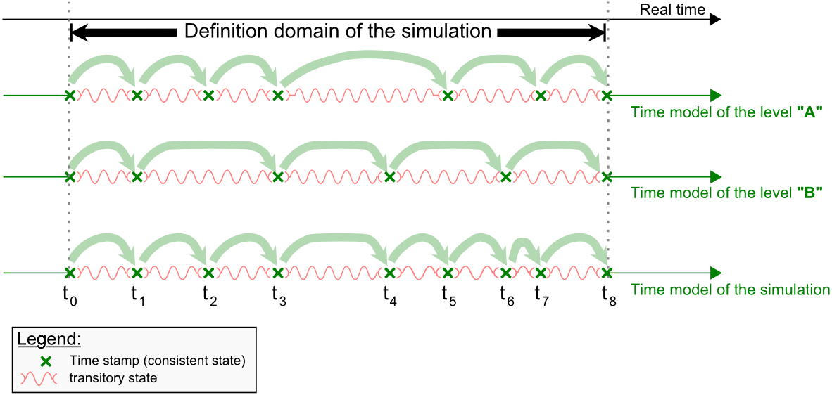
Figure 1: Illustration of a time model, for a simulation using two levels "A" and "B".The first line represents real time.The second and third line represent the time model of the levels "A" and "B". The last line represents the time model of the whole simulation. At $t_{1}$, the state of the simulation is consistent. At $t_{4}$, it is half-consistent.

From a global viewpoint, the dynamic state of the simulation is consistent (resp. transitory) if all of its levels are consistent (resp. transitory). It can also be in an intermediate situation called half-consistent state, if a level is in a consistent and another level is in a transitory state. These concepts are illustrated in Figure 1.

To clarify our speech, we write $\delta{}(t)$ the consistent (or half-consistent) dynamic state of the simulation at time $t\in\mathbb{T}$ and $\delta(]t,t^{\prime}[)$ the transitory dynamic state of the simulation between the times $t\in\mathbb{T}$ and $t^{\prime}\in\mathbb{T}$.

1.3 Multi-level inherent issues

When a simulation is in a transitory phase, each level performs operations in parallel to determine the next consistent value of their dynamic state. The transitory periods of the levels are not necessarily in sync. Therefore, each level can be at a different step of its transitory operations when an interaction occurs. This point raises the following time-related issues: 1) Determine on which dynamic states is based the decision in a level to interact with another level; 2) Determine when to take into consideration the modifications in a level resulting from an action initiated in another level; 3) Determine how to preserve the consistency of the global state of the agents despite having its update occurring after the level-dependent perceptions.

This section illustrates these issues on an example containing two levels "A" and "B", presented in Figure 2

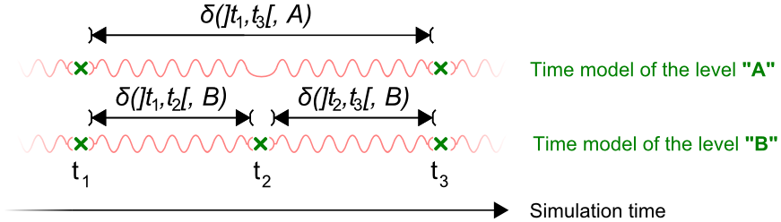
Figure 2: Illustration of a subset of a time model containing two levels "A" and "B".

1.3.1 Level interaction through perception

The first issue is related to the perception of the dynamic state of the other levels. It happens for instance at the time $t_{2}$ (see fig. 2), when an agent from the level "B" tries to read information from the level "A". Indeed, since "A" is in a transitory state at that time, the data being read by the agent might have arbitrary values. Therefore, a heuristic has to be used to disambiguate that value. For instance using the last consistent dynamic state of the level (in this case the dynamic state of "A" at the time $t_{1}$), using the arbitrary values from the transitory state at $t_{2}$ or anticipating the modifications that might have occurred in "A" between $t_{1}$ and $t_{2}$.

1.3.2 Level interaction through actions

The second issue is related to the side effects of an interaction between two levels. It happens for instance during the transitory period $]t_{1},t_{3}[$ (see fig. 2) of the level "A", if an agent from "A" tries to interact with the level "B". Indeed, since both levels have a different time scale, it is difficult to determine when the actions of "A" have to be taken for account into the computation of the dynamic state of "B". It can be during the transitory phases $]t_{1},t_{2}[$, $]t_{2},t_{3}[$ or a later one.

A generic answer to that problem might be "the next time both levels are in sync" ($t_{3}$ in this case). Yet, this leads to aberrations like taking into consideration these actions at the end of the simulation (for instance in fig 1, if an agent from the level "A" interacts with "B" during the transitory period $]t_{3},t_{5}[$).

1.3.3 Global state update

The third issue is related to the read and write access of the global state of an agent and the update of that value. Indeed, during the transitory phase of each level, the agent has to read and possibly update the value of the global states, to take into account the information that were perceived. Yet, since the perception is relative to each level, the global state is the subject of the same issues than the interactions between levels.

For instance, in figure 2, the period $]t_{1},t_{2}[$ of the simulation is a transitory period for the level "B" and a subset of the transitory period for the level "A". The latter raises the question of whether if the global state of the agent at the time $t_{2}$ has to take into consideration the data being perceived by the agent from "A" or not. Indeed, perception might not be complete at that time in "A".

1.4 Differences between multi-level approaches

There is no universal answer to the issues presented in this section, since the coherence between heterogeneous time scales is itself an ill-defined notion. The main differences between existing ML-ABM approaches are the way these issues are handled, through the answer of the following questions about the operations performed during a transitory phase $]t,t+dt[$: 1) Which agents can perform a decision during a transitory period of a level? 2) How many actions can be performed by the decision process of an agent? 3) How are committed the results of the action to the future dynamic state of a level? 4) When are performed these operations during the transitory state? 5) Which dynamic state of a level $k$ is read by a level $l$ initiating an interaction with $k$? A consistent one? A transitory one? Which ones ? 6) When is taken into account the interaction initiated by a level $l$ with a level $k$? 7) How is managed the consistency of the global state of agents?

In the next section, we present an agent-based approach called SIMILAR, that aims at addressing these issues.

2 SIMILAR

Many meta-models and simulation engines dedicated to ML-ABM have been proposed in the literature such as IRM4MLS [10], PADAWAN [11], GAMA [5] or NetLogo LevelSpace [6]. All these approaches provide a different and yet valid answer to the multi-level simulation issues. In this paper, we do not aim at detailing precisely their differences: a comprehensive survey of the different approaches can be found in [9].

Existing approaches like GAMA or PADAWAN (Pattern for Accurate Design of Agent Worlds in Agent Nests) are complete approaches providing various interesting features respectively including the agentification of emerging structures or the elicitation of interactions between agents. However, these approaches rely on a time model where the management of the potentially simultaneous actions is strongly constrained by the sequential execution of agent actions.

In this paper, we investigate another approach where agent actions are separated from their consequences in the dynamic state of the simulation, using the influence/reaction principle [3]. The resulting approach, called SIMILAR (Simulations with Multi-Level Agents and Reactions), is deeply inspired by IRM4MLS [10], a multi-level extension of IRM4S [8]. The main differences between SIMILAR and IRM4MLS are the more precise and less misleading terminology and simulation algorithms, as well as a more precise and implementation-oriented model for the reaction phase (the latter is not described in this paper due to the lack of space).

2.1 Core concepts

SIMILAR revolves around five core concepts: 1) Levels, modeling different viewpoints on the simulated phenomenon; 2) Agents lying in one or more levels. From each level where they lie, they perceive the state of one or more levels to decide how they wish to influence the evolution of the system; 3) the Environment modeling the topology, the local information (e.g. temperature) and the natural evolution of each level; 4) Influences modeling actions which effect has yet to be committed to the state of the simulation; 5) Reactions modeling how the changes depicted by the influences are committed to the state of the simulation.

We note $\mathbb{L}$ the levels defined for a simulation, $\mathbb{I}$ the domain space of all the possible influences of the simulation and $\mathbb{A}$ all possible agents of the simulation.

2.2 Heuristics

SIMILAR relies on the following heuristics and choices to manage the issues raised in the section 1.4. 1) During the transitory period $]t,t+dt_{l}[$ of a level $l\in\mathbb{L}$, the agents from $\mathcal{A}(t,l)$ decide once in parallel; 2) The number of influences produced by each decision is not constrained; 3) The result of the actions is committed to the future dynamic state of a level using a reaction mechanism [3] ; 4) During the transitory period $]t,t+dt_{l}[$ of a level $l\in\mathbb{L}$, the behavior of the agents is triggered slightly after $t$ and the reaction occurs slightly before $t+dt_{l}$; 5) The dynamic state being read by the behavior of an agent (or of the environment) is always the most recent consistent state of the level; 6) The actions emitted by an agent from a level $l$ to a level $k$ during a transitory period $]t,t+dt_{l}[$ are taken into account in the next reaction of $k$ after the time $t$ (i.e. the reaction occurring during the transitory period containing or starting with the time $t$); 7) The consistency of agent global states is attained by: i) Computing the revised global state of the agents at the beginning of the transitory period of a level (i.e. before any reaction); ii) Computing the revised global state of an agent once for all the levels starting a new transitory period at the same time; iii) Use this revised global state as the global state of the agent for the next half- consistent state of the simulation. This approach is summarized in Figure 3

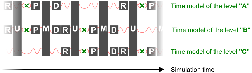
Figure 3: Illustration of the operation performed independently in each level (squares) and joint for all the levels (rectangles) during a simulation. The letters describe the type of the operation: Perception (P), Global state revision (M), Decision (D) and Reaction (R). Any arrow starting on a consistent dynamic state at a time $t$ points to the revised global state used as the new global state of the agents in the half-consistent dynamic state of the time $t$. This example focuses on the operations performed in a simulation containing one agent lying in three levels.

2.3 Dynamic state

In SIMILAR, we consider that each point of view on a phenomenon has to be embodied in a level $l\in\mathbb{L}$. As a consequence, the dynamic state $\delta(t)$ of the simulation is divided in level-specific dynamic states $\delta(t,l)$. Two kind of data can be obtained from the dynamic state of a level $l\in\mathbb{L}$: a state valuation $\sigma{}(t,l)$, defining a valuation of the level-related properties of the agents (e.g. their location or their temperature) or the environment (e.g. an ambient temperature) and the state dynamics $\gamma{}(t,l)$, defining the actions that were still being performed in that level during the observation.

$$\forall l\in\mathbb{L},\forall t\in\mathbb{T}_{l},\delta{}(t,l)=<\sigma{}(t,l),\gamma{}(t,l)>$$ (3)

2.3.1 State valuation

The state valuation $\sigma{}(t,l)$ of a level $l\in\mathbb{L}$ is the union of the local state of the environment $\phi_{\omega}(t,l)\in\Phi_{\omega}$, containing agent-unrelated information and a local state $\phi_{a}(t,l)\in\Phi_{a,l}$ for each agent $a\in\mathbb{A}$ contained in the level.

2.3.2 State dynamics

SIMILAR relies on the influence/reaction principle to model the actions resulting from the decision of the agents, from the natural evolution of the environment and the actions still being performed at time $t$. Therefore, the state dynamics $\gamma(t,l)$ of a level $l\in\mathbb{L}$ contains a set of influences.

$$\forall l\in\mathbb{L},\forall t\in\mathbb{T}_{l},\gamma(t,l)\subseteq\mathbb{I}$$ (4)

Since the data contained in an influence are mostly domain-dependent, no specific model is attached to them. They usually contain the subjects of the action (e.g. the physical state of one or more agents) as well as parameters (e.g. an amount of money to exchange).

2.4 General behavior model

The dynamic state of a simulation models a "photograph" of the simulation at time $t$. Motion is attained owing to the behavior of the agents, the natural action of the environment and the reaction of each level to influences.

2.4.1 Behavior of the agents

The behavior of an agent in a level $l\in\mathbb{L}$ has three phases: 1) Perception: extract information from the dynamic state of the levels that can be perceived from $l$; 2) Global state revision: use the newly perceived data to revise the content of the global state of the agent; 3) Decision: use the perceived data and the revised global state to create and send influences to the levels that can be influenced by $l$. Each influence models a modification request of the dynamic state of a level.

2.4.2 Natural action of the environment

The natural action of the environment is simpler than the behavior of agents: it only has one phase, where the dynamic state of the levels that can be perceived from $l$ are used to create influences sent to one or more levels that can be influenced by $l$.

2.4.3 Reaction to the influences

As in IRM4MLS, in SIMILAR the reaction of a level $l\in\mathbb{L}$ is a process computing the new consistent dynamic state of $l$. The reaction phase occurs at the end of a transitory period $]t,t+dt_{l}[$ of a level, and is computed using the value of the most recent consistent dynamic state of $l$ and the influences that were sent to $l$ during the transitory period $]t,t+dt_{l}[$;

Yet, contrary to IRM4MLS, SIMILAR provides an explicit model to the generic influences that can be found in any simulation, like the addition/removal of an agent from the simulation/a level. Such influences are called system influences, in opposition to regular influences, which are user-defined. A model is also provided to their generic reaction. These points are not detailed in this paper.

2.5 Formal notations and simulation algorithm

Not all levels are able to interact. Therefore, the interactions between levels are constrained by two digraphs: A perception relation graph $\mathbb{G}_{P}$ (resp. influence relation graph $\mathbb{G}_{I}$) defines which levels can be perceived (resp. influenced) during the behavior of the agent/environment in a specific level.

$$\begin{array}[]{lcl}\big{(}l_{1},l_{2}\big{)}\in\mathbb{G}_{P}\mbox{ (resp. }\mathbb{G}_{I}\mbox{)}&\iff&\mbox{An agent from }l_{1}\mbox{ can perceive (resp.}\\ &&\mbox{ influence) the dynamic state of }l_{2}\end{array}$$ (5)

The out neighborhood $\mathcal{N}_{P}^{+}(l)$ (resp. $\mathcal{N}_{I}^{+}(l)$) of a level $l\in\mathbb{L}$ in the perception (resp. influence) relation graph defines the levels that can be perceived (resp. influenced) by $l$.

2.5.1 Agent behavior

Since the content of the dynamic state is not trustworthy during transitory periods, the natural action of the environment and the perception of the agents are based on the last consistent dynamic state of the perceptible levels. This time is identified by the notation $floor_{l}(]t,t^{\prime}[)$, which models the last time when the dynamic state of a level $l$ was consistent for a perception occurring during a transitory period $]t,t^{\prime}[$.

$$\forall t,t^{\prime}\in\mathbb{T}^{2},\forall l\in\mathbb{L},floor_{l}(]t,t^{\prime}[)=max\Big{(}\{u\leq t|u\in\mathbb{T}_{l}\}\Big{)}$$ (6)

Based on these information, the perception phase of an agent $a\in\mathcal{A}(t,l)$ from a level $l\in\mathbb{L}$ for the transitory period $]t,t+dt_{l}[$ is defined as an application $perception_{a,]t,t+dt_{l}[,l}$. This application reads the last consistent dynamic state of each perceptible level to produce the perceived data:

$$\begin{array}[b]{p{1cm}lcl}\lx@intercol\forall l\in\mathbb{L},\forall t\in\mathbb{T}_{l}\backslash\{max(\mathbb{T}_{l})\},\forall a\in\mathcal{A}(t,l),\;\;\;\;perception_{a,]t,t+dt_{l}[,l}:\hfil\lx@intercol\\ &\prod_{k\in\mathcal{N}_{P}^{+}(l)}\Delta_{k}&\longrightarrow&\mathbb{P}_{a,l}\\ &\Big{(}\delta\big{(}floor_{k}(]t,t+dt_{l}[),k\big{)}\Big{)}_{k\in\mathcal{N}_{P}^{+}(l)}&\longmapsto&p_{a,l}(]t,t+dt_{l}[)\end{array}$$ (7)

In this notation, $\mathbb{P}_{a}$ models the domain space of the data that can be perceived by the agent $a$, from the perspective of the level $l$. It can contain raw data from the dynamic states, or an interpretation of these data. For instance, in a road traffic simulation, the drivers do not need to put the absolute position of the leading vehicle (i.e. raw data from the dynamic state) in their perceived data: the distance between the two vehicles is sufficient.

The revision of the global state of an agent $a\in\mathcal{A}(t,l)$ for a transitory period starting at the time $t$ is defined as an application $globalRev_{a,]t,t+dt[}$. This application reads the most recent consistent global state $\mu_{a}\big{(}t)$ of the agent $a$ and the perceived data $p_{a,l}(]t,t+dt_{l}[),\forall l\in\mathbb{L}|t\in\mathbb{T}_{l}$ of all the levels that started a transitory phase at the time $t$, in order to determine the value of the revised global state $\mu_{a}(]t,t+dt[)$ of the agent during the transitory period.

$$\begin{array}[b]{p{1cm}lcl}\lx@intercol\forall t\in\mathbb{T}\backslash\{max(\mathbb{T})\},\forall a\in\mathcal{A}(t),\;\;\;\;globalRev_{a,]t,t+dt[}:\hfil\lx@intercol\\ &\mathbb{M}_{a}\times\prod_{l\in\mathbb{L}|t\in\mathbb{T}_{l}}\mathbb{P}_{a,l}&\longrightarrow&\mathbb{M}_{a}\\ &\Big{(}\mu_{a}(t),\big{(}p_{a,l}(]t,t+dt_{l}[)\big{)}_{l\in\mathbb{L}|t\in\mathbb{T}_{l}}\Big{)}&\longmapsto&\mu_{a}(]t,t+dt[)\end{array}$$ (8)

Finally, the decision of an agent $a\in\mathcal{A}(t,l)$ from a level $l\in\mathbb{L}$ for the transitory period $]t,t+dt_{l}[$ is defined as an application $decision_{a,]t,t+dt_{l}[,l}$. This application reads the revised global state $\mu_{a}(]t,t+dt[)$ of $a$ and the perceived data $p_{a,l}(]t,t+dt_{l}[)$ computed for the level $l$ to create the influences that will modify levels during their respective next reaction.

$$\begin{array}[b]{p{1cm}lcl}\lx@intercol\forall l\in\mathbb{L},\forall t\in\mathbb{T}_{l}\backslash\{max(\mathbb{T}_{l})\},\forall a\in\mathcal{A}(t,l),\;\;\;\;decision_{a,]t,t+dt_{l}[,l}:\hfil\lx@intercol\\ &\mathbb{M}_{a}\times\mathbb{P}_{a,l}&\longrightarrow&2^{\mathbb{I}}\\ &\Big{(}\mu_{a}(]t,t+dt[),p_{a,l}(]t,t+dt_{l}[)\Big{)}&\longmapsto&\mathcal{I}_{a,l}(]t,t+dt_{l}[)\end{array}$$ (9)

If we note $level(i)$ the level at which the influence $i\in\mathbb{I}$ is aimed, then the influence relation graph imposes the following constraint to the decision:

$$\forall l\in\mathbb{L},\forall t\in\mathbb{T}_{l}\backslash\{max(\mathbb{T}_{l})\},i\in\mathcal{I}_{a,l}(]t,t+dt_{l}[)\Rightarrow level(i)\in\mathcal{N}_{I}^{+}(l)$$ (10)

As a result to this phase, each created influence $i\in\mathcal{I}_{a,l}(]t,t+dt_{l}[)$ is added to the transitory state dynamics of $k=level(i)$, for the transitory period $]floor_{k}(]t,t+dt_{l}[),floor_{k}(]t,t+dt_{l}[)+dt_{k}[$.

2.5.2 Natural action of the environment

The natural action of the environment from a level $l\in\mathbb{L}$ for the transitory period $]t,t+dt_{l}[$ is defined as an application $natural_{]t,t+dt_{l}[,l}$. This application reads the last consistent dynamic state of each perceptible level to create the influences that will modify the dynamic state of the influenceable levels (during their reaction).

$$\begin{array}[b]{p{1cm}lcl}\lx@intercol\forall l\in\mathbb{L},\forall t\in\mathbb{T}_{l}\backslash\{max(\mathbb{T}_{l})\},\;\;\;\;natural_{]t,t+dt_{l}[,l}:\hfil\lx@intercol\\ &\prod_{k\in\mathcal{N}_{P}^{+}(l)}\Delta_{k}&\longrightarrow&2^{\mathbb{I}}\\ &\Big{(}\delta\big{(}floor_{k}(]t,t+dt_{l}[),k\big{)}\Big{)}_{k\in\mathcal{N}_{P}^{+}(l)}&\longmapsto&\mathcal{I}_{\omega,l}(]t,t+dt_{l}[)\end{array}$$ (11)

The resulting influences are managed with the same process than the ones coming from the decisions of the agents.

2.5.3 Reaction of a level

The reaction of a level $l\in\mathbb{L}$ is computed at the end of each transitory period $]t,t+dt_{l}[$ where $t\in\mathbb{T}_{l}$. It is defined as an application $reaction_{l,]t,t+dt_{l}[}$ reading the transitory dynamic state $\delta(]t,t+dt_{l}[,l)$ of the level to determine the next consistent value of the dynamic state $\delta(t+dt_{l},l)$.

$$\begin{array}[b]{p{1cm}lcl}\lx@intercol\forall l\in\mathbb{L},\forall t\in\mathbb{T}_{l}\backslash\{max(\mathbb{T}_{l})\},\;\;\;\;reaction_{]t,t+dt_{l}[,l}:\hfil\lx@intercol\\ &\Delta_{l}&\longrightarrow&\Delta_{l}\\ &\Big{(}\delta\big{(}]t,t+dt_{l}[,l\big{)}\Big{)}&\longmapsto&\delta\big{(}t+dt_{l},l\big{)}\end{array}$$ (12)

The reaction has the following responsibilities: 1) Take into consideration the influences of $\gamma(]t,t+dt_{l}[,l)$ to update the local state of the agents, update the local state of the environment, create/delete agents from the simulation or add/remove agents from the level; 2) Determine if the influences of $\gamma(]t,t+dt_{l}[,l)$ persist in $\gamma(t+dt_{l},l)$ (if they model something that has not finished at the time $t+dt_{l}$); 3) Manage the colliding influences of $\gamma(]t,t+dt_{l}[,l)$.

2.5.4 Simulation algorithm

The simulation algorithm of SIMILAR is presented in Figure 4. It relies on the presented concepts and complies with the time constraints defined in [10].

$t\longleftarrow min(\mathbb{T})$;

$D\longleftarrow$ Map$<$level,dynamic state$>$ //Most recent consistent dynamic state

$M\longleftarrow$ Map$<$agent,memory state$>$ //Most recent consistent global state

$T\longleftarrow$ Map$<$level,time interval$>$ //Next transitory state time interval

$D_{T}\longleftarrow$ Map$<$level,dynamic state$>$ //Next transitory state

$M_{T}\longleftarrow$ Map$<$agent,memory state$>$ //Most recent revised global state

for $l\in\mathbb{L}$ do

       $D[l]\longleftarrow\delta(t,l)$;

       $T[l]\longleftarrow]t,t+dt_{l}[$;

       $D_{T}[l]\longleftarrow$ copy of $D[l]$;

      

end while $t\neq max(\mathbb{T})$ do

       for $l\in\mathbb{L}$ do

             if $t=end(T[l])$ then

                   $D[l]\longleftarrow reaction_{T[l],l}(D_{T}[l])$;

                   $D_{T}[l]\longleftarrow$ copy of $D[l]$;

                   $T[l]=]t,t+dt_{l}[$;

                  

            end for $a\in\mathcal{A}(t)$ do

                   $M[a]=$ copy of $M_{T}[a]$;

                  

            end

      end $L_{i}\longleftarrow\{l\in\mathbb{L}|start(T[l])=t\}$;

       $p\longleftarrow$ Map$<$agent,Map$<$ level, perceived data $>>$;

       $A\longleftarrow\emptyset$;

       for $l\in L_{i}$ do

             for $a\in\mathcal{A}(t,l)$ do

                   $p[a][l]\longleftarrow perception_{a,T[l],l}\big{(}(D[k])_{k\in\mathcal{N}_{P}^{+}(l)}\big{)}$;

                   $A\longleftarrow A\cup\{a\}$

            end

      end for $a\in A$ do

             $M_{T}[a]=globalRev_{a,]t,t+dt[}(M[a],p[a])$;

            

      end $I\longleftarrow\emptyset$;

       for $l\in L_{i}$ do

             $I\longleftarrow I\cup natural_{T[l],l}\big{(}(D[k])_{k\in\mathcal{N}_{p}^{+}(l)}\big{)}$;

             for $a\in\mathcal{A}(t,l)$ do

                   $I\longleftarrow I\cup decision_{a,T[l],l}(M_{T}[a],p[a])$;

                  

            end

      end for $i\in I$ do

             Add $i$ to the state dynamics of $D_{T}[level(i)]$;

            

      end $t\longleftarrow min\Big{(}\big{\{}right(T[l]),l\in\mathbb{L}\big{\}}\Big{)}$ //$t$ becomes equal to $t+dt$

      

end

Figure 4: The simulation algorithm used in SIMILAR

Conclusion and perspectives

In this paper, we elicited several issues about time and consistency raised in multi-level simulations. There is no clear solution to theme since the notion of time consistency among heterogeneous time models is itself ill-defined. Therefore, rather than distinguishing the "right" or "wrong" approaches, we defined a theoretical frame giving a better understanding of the choices underlying each approach. Then, it is up to modelers and domain specialists to tell if these choices are appropriate or not for the study of a given phenomenon.

To cope with the multi-level related issues, we introduced a meta-model named SIMILAR based on the influence/reaction principle. This model is designed to reify as much as possible the concepts involved in the abovementionned issues, thus providing a better support to the definition of explicit solutions to them. SIMILAR includes a generic and modular formal model, a methodology and a simulation API preserving the structure of the formal model. Thus, the design of simulations is in addition more robust to model revisions and relies on a structure fit to represent the intrinsic complexity of the simulated multi-level phenomena.

SIMILAR has been implemented in Java and is available under the CeCILL-B license.

It is available at http://www.lgi2a.univ-artois.fr/~morvan/similar.html.

References

- [1] B. Camus, C. Bourjot, and V. Chevrier. Considering a multi-level model as a society of interacting models: Application to a collective motion example. Journal of Artificial Societies & Social Simulation, 18(3), 2015.
- [2] D. David and R. Courdier. See emergence as a metaknowledge. a way to reify emergent phenomena in multiagent simulations? In Proceedings of ICAART’09, pages 564–569, Porto, Portugal, 2009.
- [3] J. Ferber and J-P. Müller. Influences and reaction: a model of situated multiagent systems. In 2nd International Conference on Multi-agent systems (ICMAS’96), pages 72–79, 1996.
- [4] J. Gil-Quijano, T. Louail, and G. Hutzler. From biological to urban cells: Lessons from three multilevel agent-based models. In Principles and Practice of Multi-Agent Systems, volume 7057 of LNCS, pages 620–635. Springer, 2012.
- [5] A. Grignard, P. Taillandier, B. Gaudou, D. A. Vo, N. Q. Huynh, and A. Drogoul. GAMA 1.6: Advancing the art of complex agent-based modeling and simulation. In PRIMA 2013: Principles and Practice of Multi-Agent Systems, volume 8291 of LNCS, pages 117–131. Springer, 2013.
- [6] A. Hjorth, B. Head, and U. Wilensky. Levelspace netlogo extension. http://ccl.northwestern.edu/rp/levelspace/index.shtml, 2015.
- [7] T. Huraux, N. Sabouret, and Y. Haradji. A multi-level model for multi-agent based simulation. In Proc. of 6th Int. Conf. on Agents and Artificial Intelligence (ICAART), 2014.
- [8] F. Michel. The IRM4S model: the influence/reaction principle for multiagent based simulation. In Proc. of 6th Int. Conf. on Autonomous Agents and Multiagent Systems (AAMAS), pages 1–3, 2007.
- [9] G. Morvan. Multi-level agent-based modeling - a literature survey. CoRR, abs/1205.0561, 2013.
- [10] G. Morvan, A. Veremme, and D. Dupont. IRM4MLS: the influence reaction model for multi-level simulation. In Multi-Agent-Based Simulation XI, volume 6532 of LNCS, pages 16–27. Springer, 2011.
- [11] S. Picault and P. Mathieu. An interaction-oriented model for multi-scale simulation. In Proc of the 22nd Int. Joint Conf. on Artificial Intelligence, pages 332–337. AAAI Press, 2011.
- [12] D-A. Vo. An operational architecture to handle multiple levels of representation in agent-based models. PhD thesis, Université Paris VI, 2012.