Faraday rotation in GRMHD simulations of the jet launching zone of M87

Abstract

Non-VLBI measurements of Faraday rotation at mm wavelengths have been used to constrain mass accretion rates ($\dot{M}$) onto supermassive black holes in the centre of the Milky Way and in the centre of M87. We constructed general relativistic magnetohydrodynamics models for these sources that qualitatively well describe their spectra and radio/mm images invoking a coupled jet-disk system. Using general relativistic polarized radiative transfer, we now also model the observed mm rotation measure (RM) of M87. The models are tied to the observed radio flux, however, electron temperature and accretion rate are degenerate parameters and are allowed to vary. For the inferred low viewing angles of the M87 jet, the RM is low even as the black hole $\dot{M}$ increases by a factor of $\simeq 100$. In jet-dominated models, the observed linear polarization is produced in the forward-jet, while the dense accretion disk depolarizes the bulk of the near-horizon scale emission which originates in the counter-jet. In the jet-dominated models, with increasing $\dot{M}$ and increasing Faraday optical depth one is progressively sensitive only to polarized emission in the forward-jet, keeping the measured RM relatively constant. The jet-dominated model reproduces a low net-polarization of $\simeq 1$ per cent and RMs in agreement with observed values due to Faraday depolarization, however, with $\dot{M}$ much larger than the previously inferred limit of $9\times 10^{-4}\,\rm M_{\odot}yr^{-1}$. All jet-dominated models produce much higher RMs for inclination angles $i\gtrsim 30^{\circ}$, where the line-of-sight passes through the accretion flow, thereby providing independent constraints on the viewing geometry of the M87 jet.

1 Introduction

Synchrotron radiation is intrinsically linearly polarized. If the wave passes through a magnetized plasma (a Faraday screen) the plane of polarization rotates. The degree of rotation is wavelength-dependent, with an observable rotation measure (RM) given by,

$$RM=\frac{\chi(\lambda_{1})-\chi(\lambda_{2})}{\lambda_{1}^{2}-\lambda_{2}^{2}}$$ (1)

where $\chi$ is the position angle of the polarization plane and $\lambda_{1}$ and $\lambda_{2}$ are two closely spaced observing wavelengths. The Faraday rotation can be also expressed in terms of the Faraday screen’s density and magnetic field strength integrated along the line of sight:

$$RM=10^{4}\frac{e^{3}}{2\pi m_{\rm e}^{2}c^{4}}\int f_{\rm rel}n_{e}B_{||}dl\,\,\,{\rm[rad\,m^{-2}]}$$ (2)

where $n_{\rm e}$ and $B_{\rm||}$ are the electron density (${\rm cm^{-3}}$) and magnetic field component projected onto the line of sight (Gauss), respectively, and $dl$ is the line element (cm) (Gardner & Whiteoak, 1966). For a relativistically cold plasma $f_{\rm rel}=1$, where the plasma electrons are relativistically hot ($\Theta_{\rm e}\equiv k_{B}T_{e}/m_{e}c^{2}>1$), the correction term becomes $f_{\rm rel}=\log(\Theta_{\rm e})/2\Theta_{\rm e}^{2}$ and the rotation is suppressed (e.g., Jones & Odell 1977). Notice that Eq. 2 is valid only if $\chi(\lambda)\sim\lambda^{2}$, which is satisfied for a Faraday optical depth $\tau_{\rm FR}=\int dl\rho_{V}\ll 1$, where $\rho_{V}$ is the Faraday rotation coefficient.

The effect of Faraday rotation is commonly used to probe the plasma and magnetic field strengths and directions in various astronomical objects, e.g., in Active Galactic Nuclei (AGN) jets (Anderson et al., 2015), in jet radio lobes (e.g., Feain et al. 2009), in galaxy clusters (Feretti et al., 2012) and in ionized gas of the interstellar medium (Haverkorn & Spangler, 2014).

There are a few measurements of RM near supermassive black holes. In Sgr A*, the Galactic center black hole, the measured $RM=-5\times 10^{5}{\rm rad\,m^{-2}}$ (Bower et al. 2003, Marrone et al. 2007) and $RM=-7\times 10^{4}{\rm rad\,m^{-2}}$ is found at the Bondi scale a few arcseconds away (Eatough et al., 2013). Other black holes with RM detections include 3C 84 with $RM=8\times 10^{5}\,{\rm rad\,m^{-2}}$ (Plambeck et al., 2014), the core of M87 (hereafter M87*) with $RM<2\times 10^{5}\,{\rm rad\,m^{-2}}$ (Kuo et al., 2014), and PKS 1830-211 with $RM\approx 10^{7}\,{\rm rad\,m^{-2}}$ (Martí-Vidal et al. 2015, where the observation possibly probes plasma 0.01 parsec away from the black hole).

All these RM are measured at millimetre wavelengths with non-VLBI observations, so that the sources are not resolved. In Sgr A*, M87*, and 3C 84, the measured RM was then used to constrain the mass accretion rate onto the central object (e.g., Bower et al. 1999). The usual procedure to interpret the observed RM is to integrate Eq.2 in the radial direction with a power-law profile for $n_{e}$ and $B$ (usually from equipartition condition) from a semi-analytical advection dominated accretion flow model (ADAF, e.g., Narayan et al. 1998). The accretion rate onto the black hole is then provided by the ADAF model (Marrone, 2006). Based on this model, the measured RM from Sgr A* of $-5.6\pm 0.7\times 10^{5}\rm rad\rm m^{-2}$ was used to estimate $\dot{M}=5\times 10^{-9}-2\times 10^{-7}\,\rm M_{\odot}yr^{-1}$ where the lower and upper limits are for different slopes of the electron density radial profiles which depend on the presence and properties of an outflow assumed to be produced by accretion process (Bower et al., 2003; Marrone, 2006; Marrone et al., 2007). In a similar fashion, the upper limit for the M87* of $|RM|<7.5\times 10^{5}\rm rad\rm m^{-2}$ have led to an accretion rate constraint of $\dot{M}<9\times 10^{-4}\,\rm M_{\odot}yr^{-1}$ (Kuo et al. 2014, Li et al. 2016).

These accretion rate constraints assume that the polarized emission is produced close to the black hole and then is Faraday rotated in the extended accretion flow. In Sgr A*, the compact emission region (Doeleman et al., 2008), observed scaling of $\chi\sim\lambda^{2}$, and $\simeq 10$ per cent RM variability (Marrone et al., 2007) support this scenario. In other sources, especially M87*, the emission near the black hole may not be produced by an accretion flow such as an ADAF, but, e.g., by a jet, so that the existing measurements would be probing the plasma flowing out from the central region. One also has to keep in mind that in case of black holes their accretion flow is simultaneously the source of synchrotron radiation and the Faraday screen (e.g., Beckert & Falcke 2002). The polarization plane position angle $\chi$ does not have to be constant with $\lambda^{2}$ as if it was if the polarized source is behind an ’external’ Faraday screen. This is because the accretion flow has a complex structure where self-absorption and depolarization of radiation take place. Finally, the $\chi$ may be additionally alternated by interstellar medium in the host galaxy. All above suggest that observed $\chi(\lambda)$ should be interpreted carefully.

In this work, we present polarized emission models based on combining an ADAF-like model realized in three-dimensional general relativistic magnetohydrodynamics (3-D GRMHD) simulations with polarized radiative transport ray-tracing calculations near a Kerr black hole. The radiative transfer model predicts the synchrotron maps of the plasma appearance near the black hole in all Stokes parameters (I,Q,U,V) at various wavelengths. We can therefore calculate what is the change of $\chi\equiv arg(Q+iU)/2$ as a function of wavelength and compute the model RM using Eq. 1, without using approximate formulas, such as Eq. 2. Contrary to previous RM modeling, in the present RM model all relativistic effects will be included: the observer viewing angle effects and the magnetic field geometry are naturally taken into account and the mass accretion rate onto the black hole is self-consistently calculated within the GRMHD simulation.

Past studies of polarized radiative transfer through GRMHD simulations (e.g., Broderick & McKinney 2010, Shcherbakov et al. 2012, Gold et al. 2016, Dexter 2016) mostly focused on models of linear polarization $LP\equiv\sqrt{Q^{2}+U^{2}}$ and circular polarization ($V$) from the Galactic center black hole Sgr A*. Only Broderick & McKinney (2010) shows RM maps based on GRMHD simulations of the M87 jet but these are done at low frequencies (15 GHz) for solutions extrapolated to large distances from the black hole. To our knowledge there are no GRMHD polarized images of the M87* at millimetre wavelengths. Hence our study focuses on 3-D GRMHD models that were applied to the M87* by Mościbrodzka et al. (2016) (hereafter M16), where we studied only unpolarized intensity of radiation at various wavelengths.

Here we show that the low net linear polarization and RM of M87* (Kuo et al., 2014) are in good agreement with the expectations from those models that best match the observed properties of the radio jet. The total intensity submm-wave image arises from the counter-jet, due to strong light bending effects. This emission is depolarized by Faraday rotation in the dense, cold accretion disk. As a result, the net polarization mostly originates in the forward jet, which produces little flux, leading to a low total net polarization fraction and RM values consistent with the observed upper limits. The accretion rate in the models can be much larger than found from the semi-analytical ADAF RM modeling, since the RM originates in the forward jet rather than in the accretion flow itself.

The paper is organized as follows. In Sect. 2 we briefly describe the GRMHD simulation. The radiative transfer models are described in Sect. 3. We present our results in Sect. 4 and summarize them in Sect. 5.

2 Model of accretion flow and jet

The details of the GRMHD model scaled to M87* are described in M16. The simulations follow the evolution of a hot accretion accretion flow in the equatorial plane of a spinning, supermassive black hole. The black hole angular velocity is $a_{*}\approx 0.94$. The accretion disk and the black hole are driving magnetized jets that are roughly aligned with the spin axis of the black hole. The model studied here is refered as to SANE in the current jargon (which stand for Standard And Normal Evolution), having low-power jets. The models extend in radius from the black hole event horizon to 240 $R_{g}$.

The GRMHD simulations provide only the fluid pressure, which is dominated by the protons. In a perfect fluid, the pressure in a grid zone gives a proton temperature. For underluminous accretion flows, protons and electrons are not necessarily well coupled. We have to assume an electron temperature as they are not self-consistently computed in the GRMHD simulations, yet they are essential in calculating synchrotron emission. The electron temperature is parameterized by a coupling ratio, $T_{\rm p}/T_{\rm e}$ , between proton and electron temperature. We study a class of models in which both the proton-to-electron temperature ratio and the mass accretion rate onto the black hole are allowed to vary. For each temperature ratio we adjust the mass accretion rate onto the black hole (which is achieved by multiplying the plasma density by a constant number) so that the total flux emitted at mm wavelengths is equal to 1 Jansky, consistent with mm observations of the source (Doeleman et al. 2012, Kuo et al. 2014).

In addition, $T_{\rm p}/T_{\rm e}$ depends on plasma magnetization. Following M16 we assume that the electron temperature is

$$\frac{T_{\rm{p}}}{T_{\rm{e}}}=R_{\rm{high}}\frac{\beta^{2}}{(1+\beta^{2})}+R_{\rm{low}}\frac{1}{(1+\beta^{2})}$$ (3)

where plasma $\beta=P_{\rm{gas}}/P_{\rm{mag}}$ and $P_{\rm{mag}}=B^{2}/2$. $R_{\rm{high}}$ and $R_{\rm{low}}$ are temperature ratios that parametrize the electron-to-proton coupling in the weakly magnetized regions (disk, high $\beta$ regions) and strongly magnetized regions (jet, low $\beta$ regions), respectively. We assume constant $R_{\rm low}=1$ and we vary $R_{\rm high}$. Since the nature of the mm-wave emission in the M87* is unknown, our goal is to smoothly transition from the disk emission dominated models (in which the electrons are strongly coupled to protons everywhere) to the jet emission dominated models (in which the electrons are strongly coupled to proton in the jet region and weakly coupled to protons in the disk zone).

In this paper we consider models with $R_{\rm low}=1$ and $R_{\rm high}=1,5,10,20,40,100$. This is the same as the models studied in M16, for which the corresponding accretion rates are $\dot{M}=1\times 10^{-4},4\times 10^{-4},1\times 10^{-3},3\times 10^{-3},5\times 10^{-3},9\times 10^{-3}\,\rm M_{\odot}yr^{-1}$, respectively. The models are listed in Table 1.

In all models, the observer viewing angle is fixed to $i=20\degr$ from the black hole spin axis consistent with observations of the large scale jet (Mertens et al., 2016). The 1 mm emission maps based on unpolarized radiation transfer are presented in our previous work. Notice that model RH100 is consistent with the broadband emission observed in M87* and the images of this model resemble the VLBI observations of the source at 7 and 3.5mm. RH100 is therefore currently our best-bet model for the M87*.

3 Model of polarized radiation

Polarized synchrotron emission is computed with the fully general relativistic polarized radiative transfer ray-tracing scheme grtrans (Dexter & Agol, 2009; Dexter, 2016). This public code has been extensively tested which makes it the current standard of the general relativistic polarized radiative transfer models. The code includes approximate synchrotron emission and absorption coefficients in all Stokes parameters, as well as Faraday rotation and conversion (Shcherbakov, 2008) suitable for thermal plasmas as modeled here.

The result of the calculation are the intensity maps overplotted with polarization angle $\chi$ at two closely spaced frequencies around 230 GHz (220, 240GHz) as a function of coordinates on the sky. We use these $\chi$-maps to calculate maps of RM. The maps show the inner 26 $GMc^{-2}$ in the plane of the black hole where the most of emission at this wavelength comes from. We also integrate the maps with Stokes parameters to simulate non-VLBI observables that are currently available.

Faraday rotation depends on the plasma Faraday optical depth defined here as $\tau_{\rm FR}=\int\rho_{V}dl$, where $\rho_{V}=4\pi e^{3}/m_{e}^{2}c^{2}n_{e}Bf/\nu^{2}$ is the plasma rotativity. Formally $f$ is a function of electron temperature $\Theta_{e}=k_{B}T_{e}/m_{e}c^{2}$, $\nu$, and $B$ (see Eq. B16 in Appendix B2 in Dexter 2016) but approximately $f\approx\Theta_{e}^{-2}$. Varying $R_{\rm high}$ from 1 to 100 corresponds to increasing $f$ by a factor of $10^{4}$. In our models the plasma density scales with the accretion rate and $n_{e}\propto\dot{M}$ and the magnetic field strength scales as $B\propto\dot{M}^{1/2}$ ($\beta=\rm const.$). In all models, $\nu=230$ GHz and $dl\approx 100R_{g}=100GM_{\rm BH}/c^{2}=9\times 10^{16}$ cm are fixed. Hence, $\tau_{\rm FR}\propto\dot{M}^{3/2}/T^{2}$ or $\dot{M}^{3/2}R_{\rm high}^{2}$. In model RH1, $n_{e}=10^{4}\,{\rm cm^{-3}}$, $B=0.1$ Gauss, and $\Theta_{e}=50$ so the expected model Faraday depth is about $\tau_{\rm FR}\approx 1$. But in model RH100, the expected $\tau_{\rm FR}\approx 10^{6}$. In the models considered here, the Faraday optical depth changes from less than unity to extremely high values. Since the polarization vector $\chi$ oscillates every $\tau_{\rm FR}=2\pi$, this means that in extreme cases $\chi$ will rotate by $\sim 10^{6}\times 2\pi$ over small distances.

The radiative transfer equations become stiff when $\Delta\tau>1$ to any transfer coefficient between sampled geodesic points, and we find that an integrator for stiff equations (ODEPACK integrator LSODA, Hindmarsh, 1983) fails when $\Delta\tau\gtrsim 100$, a condition often reached in the high accretion rate models even when using an enormous number of points on each geodesic, $n=25600$. The analytic solutions for Faraday rotation are oscillatory in (Q,U,V). Failing to converge causes the amplitude of the oscillations to grow, which can produce enormous positive or negative intensities, and/or polarization fractions much larger than 100 per cent. Shcherbakov et al. (2012) got around this problem in low frequency models of Sgr A* by integrating “spherical” polarized Stokes parameters rather than (Q,U,V). In the spherical Stokes parameters, the amplitude and phase of the oscillatory Faraday solutions are integrated separately. Rapid variations of Faraday depth between zones then lead to convergence difficulties in the phase, but do not cause failures in the integration. The form of the polarized radiative transfer equations in spherical Stokes parameters is given in Appendix A, which we have implemented in grtrans.

A reliable RM solution of the radiative transfer equations has to be accurate to $\ll 1$ per cent to not miss entire rotations of the polarization vector. The radiative transfer solutions are converged down to 1 per cent as demonstrated in Dexter (2016) but in case of problems with moderate Faraday depths ($\tau_{\rm FR}\leq 100$). In the limit of very large $\tau_{\rm FR}$ the polarization angle and degree do not converge with the number of points on a geodesic. We instead calculate mean values and error bars averaged over a number of runs.

4 Results

4.1 Convergence of radiative transfer solutions

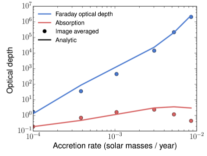
Figure 1: Absorption and Faraday rotation optical depths as a function of accretion rate measured from intensity-weighted averages of all rays in the images (points) and estimated using $\tau_{\rm FR}\propto\dot{M}^{3/2}/T_{\rm disk}^{2}$ and $\tau_{\rm abs}\propto\dot{M}^{3/2}T$ (solid lines), scaled to the lowest $\dot{M}$ result. Models with lower disk temperature require higher accretion rates (M16), leading to rapidly increasing Faraday optical depth with accretion rate for these models while the absorption stays roughly constant.

Figure 1 shows the expected vs. measured absorption and Faraday rotation optical depth along the line of sight. The “analytic” curve is from the model $\dot{M}$ and $T_{disk}$, relative to the RH1 model, e.g. $\tau_{\rm FR}\propto\dot{M}^{3/2}/T^{2}$, $\tau_{\rm abs}\propto\dot{M}^{3/2}T$, where the scaling for absorption optical depth with $\dot{M}$ could also be $\dot{M}^{2}$. The measured curves are from intensity-weighted averages along rays, which are then also intensity-weighted across the images. This shows how the Faraday rotation optical depth grows dramatically with lowering disk temperature, and is $\gg 1$ in all cases but RH1. The absorption on the other hand gets important in the lower $T_{disk}$ models, but stays much smaller than the Faraday optical depth.

It is necessary to demonstrate that the radiative transfer calculations are fully converged in sense that numerical errors do not have a significant contribution to the final result. To calculate the RM correctly, we need to have maps converged in all Stokes parameters at nearby frequencies of interest. We check how well the solutions agree when simulating images with increasing number of points along the geodesics, $n$ (logarithmically spaced within 50M from the black hole). In particular we consider two models with $n=32000$ and $n=50000$ and calculate relative difference between them.

Table 1: Convergence of radiative transfer based on models at $\nu_{1}=$230 GHz with n=32000 and n=50000. Image resolution in all models is $256^{2}$ pixels. Columns 1 and 2 show the model ID and model mass accretion rate. Columns 3 through 6 shows the difference between image integrated values in two runs with different number of integration points along geodesics lines. Column 7 shows the change of the polarization angle between $\nu_{1}=$230 and $\nu_{2}=$240 GHz. Column 8 shows mean Faraday rotation between the two frequencies with errorbars from runs with n=8000, 16000, 32000, 50000 of integration points along the geodesics. Columns 9 and 10 show the total linear and circular polarization degrees of the model.

ID	$\dot{M}$ [$\frac{M_{\odot}}{yr}$]	$\frac{\Delta I_{tot}}{I_{tot}}$	$\frac{\Delta LP_{tot}}{LP_{tot}}$	$\frac{\Delta V_{tot}}{V_{tot}}$	$\Delta\chi_{tot}$ [rad]	$\chi_{tot,\nu_{1}}-\chi_{tot,\nu_{2}}$[rad]	$\frac{\rm RM}{10^{5}}$ [${\rm\frac{rad}{m^{2}}}$ ]	$\frac{LP_{tot}}{I_{tot}}$ [%]	$\frac{CP_{tot}}{I_{tot}}$ [%]
(1)	(2)	(3)	(4)	(5)	(6)	(7)	(8)	(9)	(10)
RH1	$1\times 10^{-4}$	$1.4\times 10^{-3}$	$1.6\times 10^{-3}$	0.7	$9.1\times 10^{-4}$	$-3.8\times 10^{-2}$	$-2.75\pm 0.019$	4.6	-0.17
RH5	$4\times 10^{-4}$	$2.9\times 10^{-3}$	$2.4\times 10^{-2}$	$9\times 10^{-2}$	$4.4\times 10^{-3}$	$-7.6\times 10^{-2}$	$-5.2\pm 0.2$	0.7	2.04
RH10	$1\times 10^{-3}$	$3.6\times 10^{-3}$	$1.3\times 10^{-2}$	$7.3\times 10^{-2}$	$1.9\times 10^{-3}$	$-9.6\times 10^{-2}$	$-7.2\pm 0.7$	0.3	4.2
RH20	$3\times 10^{-3}$	$5.6\times 10^{-3}$	$3.9\times 10^{-2}$	0.35	$-9.7\times 10^{-3}$	$3.5\times 10^{-2}$	$2.44\pm 0.08$	1.9	1.3
RH40	$5\times 10^{-3}$	$4.7\times 10^{-3}$	$0.14$	0.35	$2.9\times 10^{-2}$	$-2.5\times 10^{-2}$	$-1.5\pm 0.24$	2.3	1
RH100	$9\times 10^{-3}$	$3.6\times 10^{-3}$	$2.2\times 10^{-2}$	0.33	$-5.1\times 10^{-2}$	$-6.6\times 10^{-2}$	$-1.85\pm 2.9$	1	1.1

Table 1 gathers results of our convergence study. We compute relative differences between image integrated $I_{\rm tot}$, $LP_{\rm tot}\equiv\sqrt{Q_{\rm tot}^{2}+U_{\rm tot}^{2}}$, $V_{\rm tot}$, and $\chi_{\rm tot}\equiv arg(Q_{\rm tot}+iU_{\rm tot})/2$ computed for two runs with different number of radiative transfer integration points along the geodesics. We find that all maps of I shown in Figure 7 computed with fully polarized transfer model are consistent with unpolarized images presented in M16. We find $\sim 0.1$ per cent convergence in Stokes I, in all cases. For cases with very high Faraday optical depth, LP and V are poorly converged. In some models, e.g., RH 40, the relative difference between the image integrated V can be as large as 35 per cent when $V\simeq 1\%$.

4.2 Faraday rotation measure dependency on $\dot{M}$ and disk temperature

We calculate $\chi_{\rm tot}$ which can be used to compute RM as expected from of non-VLBI observations. The $\chi_{\rm{tot},\nu_{1}}-\chi_{\rm{tot},\nu_{2}}$ in the Table 1 is change of total LP angle between 230 and 240 GHz. Based on that we compute RM. The errorbars of RM is a deviation from average RM computed based on with models with n=8000, 16000, 32000, and n=50000 integration points along the geodesics. The errorbars, as expected, increase with model Faraday depth. Figure 2 illustrates the model RM as a function of mass accretion rate onto the black hole. These are compared with the Kuo et al. (2014) M87* measurement and the analytic expectation $\tau_{\rm FR}\sim\dot{M}^{3/2}M_{\rm BH}^{-1/2}$ from external Faraday rotation in a cold accretion flow. We find that the self-consistently computed RM first slowly increases and then decreases with increasing mass accretion rate and $R_{\rm high}$. The exact rate of the initial increase of RM will depend on details of the electron temperature model. In the present set up, models with mass accretion rate $>9\times 10^{-4}\rm M_{\odot}yr^{-1}$ are consistent with non-VLBI observations of the M87*. Faraday RMs based on our fully self-consistent calculations significantly differ from those computed using Eq. 2 and shown in Figure 2 as red dots.

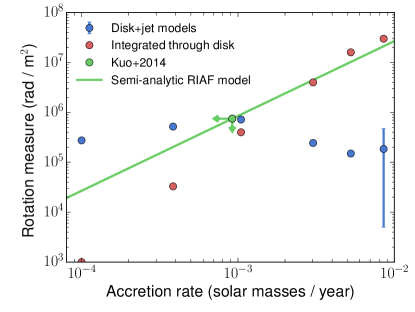
Figure 2: Rotation measure as a function of accretion rate onto the black hole. The analytically calculated Faraday depth follows a $\tau_{\rm FR}\sim\dot{M}^{3/2}M_{\rm BH}^{-1/2}$ relation, based on a model in which the synchrotron source is behind an external Faraday screen (Marrone, 2006). Data points are from our simulations summarized in Table 1. The data point with an arrow is the observed upper limit for RM from Kuo et al. (2014). RMs computed using Eq. 2 are marked as “integrated through disk”.

Moving from the disk emission dominated models (RH1) to jet emission dominated models (RH40, RH100) the accretion rate increases but at the same time the electron temperature in the disk decreases, which shifts the emission region closer towards the jet where the electrons remain relativistically hot. In model RH40, the millimetre emission (Stokes I) is predominantly produced by the jet sheath. The emission from the jet sheath is produced just near the event horizon of the black hole at the jet launching point. For a viewing angle of 20 degrees an external observer sees a ring of emission around the shadow of the black hole that is a gravitationally lensed image of the counter-jet. Weak emission from the forward jet can also be noticed. This is illustrated in Figure 3. The counter jet dominates the emission because it arises at a small projected separation from the black hole, where the light bending effects are strong and the beaming comes from the orbital rather than radial velocity (Dexter et al., 2012). For comparison we also plot an image from the force-free jet model of Broderick & Loeb (2009). The model parameters are the same as for their M0 model, but with a footpoint radius of $r_{\rm fp}=2$M, for better agreement with the compact observed 230 GHz size of M87* (Doeleman et al., 2012). Figure 4, shows the significant difference in polarization structure between both models. Spatially resolved polarization observations could distinguish between the Broderick & Loeb (2009) forward jet and the RH40 counter-jet models.

Synchrotron radiation is intrinsically highly polarized (up to 100 per cent, e.g., Pandya et al., 2016), but in our images the brightest regions (in Stokes I) are depolarized to 10 per cent and the total linear polarization degree is 1 per cent on average (in all models except in model RH1, see the last column in Table 1). What is causing the strong depolarization? We recompute model RH40 using lower and upper hemispheres of the GRMHD simulations to investigate the polarimetric properties of light coming from the counter-jet and forward-jet, respectively. Fig. 5 shows the structure of linear polarization intensity and orientation of the polarization plane of the counter- and forward-jet. In Fig. 5, the counter jet polarization (first panel) is evidently significantly scrambled compared to coherent signal from the forward jet (second panel). The total LP degree from the counter-jet is 1 per cent. This is smaller than the total polarization degree of the forward-jet which is 3.1 per cent. The forward to counter jet LP flux ratio is about 2.2. In Fig. 5 third and fourth panels, both models are then recomputed assuming zero Faraday rotation and conversion $\rho_{\rm QV}=0$ in Eq. 6. Notice that if $\rho_{\rm QV}=0$ the polarization ticks are organized in both counter- and forward- jet. Without Faraday effects, the forward to counter jet LP flux ratio is 1.1 indicating that indeed the Faraday effects depolarize the counter jet emission and scramble its polarization structure. Here, the total LP degree is 3 and 6 percent for counter and forward-jet respectively. Total low polarization degree in models with $\rho_{\rm QV}=0$ are due to a varying magnetic field structure across the image (“beam depolarization”).

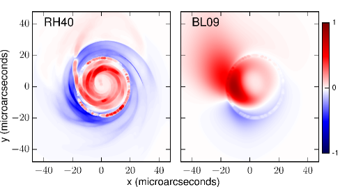
Figure 3: Intensity for each image pixel originating from below (blue) and above (red) the midplane for the RH40 (left) and BL09 (right) models. Each image is scaled linearly to its maximum intensity. The forward jet, above the midplane, produces most of the observed emission in the BL09 case. In the RH40 case, the bulk of the flux density originates in the counter-jet, with a contribution from the forward jet.

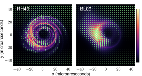
Figure 4: Intensity (colors) and polarization maps (ticks) for model RH40 (left) and a semi-analytic force-free jet model (right, Broderick & Loeb, 2009, BL09). Each image is scaled linearly to its maximum intensity. The strong Faraday rotation through the accretion disk leads to a scrambled polarization pattern in the RH40 case, while the force-free jet shows coherent polarization which traces its helical magnetic field structure. The BL09 model has much higher net polarization ($\simeq 15$ per cent compared to $\simeq 1$ per cent for RH40), which is not seen in SMA observations of M87* (Kuo et al., 2014).

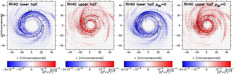
Figure 5: First and second panels: polarized emission $\sqrt{Q^{2}+U^{2}}$ for each pixel originating from below (blue) and above (red) the midplane together with polarization ticks for model RH40. Third and fourth panels: same as first and second panels but with Faraday effects switched off. The model without Faraday effects shows coherent polarization signals from both counter- and forward-jet.

If the majority of the observed LP in model RH40 is produced by the forward jet (because the counter-jet is depolarized) then the observed RM is probing the plasma conditions in the forward-jet. The effect is illustrated in Figure 6. The left panel in Figure 6, shows the total intensity maps (orange) with linear polarization ticks at 230 GHz. The middle panel in Figure 6 show maps of RMs computed using Eq. 1. The values of RM in the middle panel are up to about $10^{7}\,{\rm rad\,m^{-2}}$. In Figure 6 (right panel), we show the RM map weighted with LP to show how the observed linearly polarized emission is affected by Faraday rotation effects. This indicates that the polarized emission that is supposed to be strongly Faraday rotated is depolarized, and we pick up signals only from the polarized emission in front of the accretion disk that experiences much weaker Faraday rotation. As a consequence the measured RM is fairly independent of the disk density ($\dot{M}$) or temperature ($R_{\rm high}$).

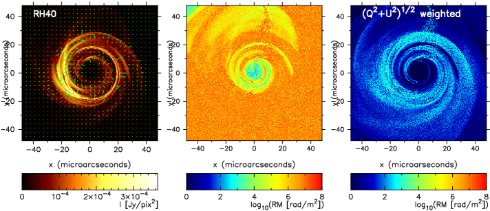
Figure 6: Left panel: Intensity map of model RH40 at 230 GHz overplotted with linear polarization $\chi$ ticks. Middle panel: RM computed from maps as in the left panel at two frequencies 230 and 240 GHz. The right panel: the same as middle panel but RM map is weighed with linear polarization $\sqrt{Q^{2}+U^{2}}$ to demonstrate how the observed linearly polarized emission is affected by Faraday rotation.

Which other models RH1-RH100 are, similar to RH40, dominated by Faraday rotation effects and in which models is the RM due to the forward jet? Figs. 7 and 8 show how polarization structure and Faraday depth change when increasing the accretion rate and decreasing the temperature of the plasma in the accretion disk (going from model RH1 to RH100). In Figure 7, the LP gets scrambled staring from model RH5 for which $\tau_{\rm FR}>10$. Figure 8 shows the absolute value of the intensity-weighted Faraday optical depth along light rays (colors, with blue and yellow contours at $\tau_{\rm FR}=1,100)$ and polarization maps for the same models. We find that the polarization gets scrambled for lines of sight outside the photon ring (bright rings of large Faraday depth). In the RH20 model, every line of sight of interest has a Faraday depth > 100. We conclude that in models RH20 through RH100, the depolarization is dominated by Faraday rotation that is occurring in the disk, while the observed polarization and RM are produced in the forward jet and are therefore independent of the accretion disk model parameters. The possibility that the RM originates in the jet rather than the extended accretion flow is natural given the low inclination of M87 jet, and was considered previously (Kuo et al., 2014; Li et al., 2016; Feng et al., 2016). We have demonstrated this with self-consistent MHD disk+jet models that can match the radio observations.

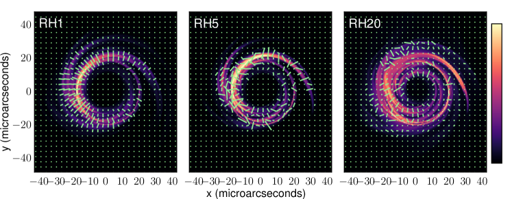
Figure 7: Intensity maps of model RH1-20 at 230 GHz overplotted with linear polarization $\chi$ ticks. Each image is scaled linearly to its maximum intensity. The polarization pattern in the RH1 model varies smoothly over the image. The other models have lower disk electron temperatures and higher accretion rates. The resulting large Faraday optical depth through the disk scatters the polarization for lines of sight to the bright, lensed counter-jet.

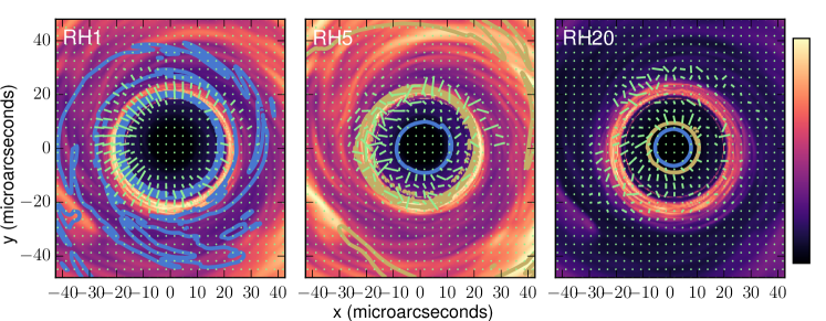
Figure 8: Faraday rotation maps (colors) with polarization ticks. The blue and yellow contours are $\tau_{\rm FR}$ = 1 and 100, respectively. In RH1 many lines of sight are Faraday thin, leading to a coherent polarization map tracing the underlying magnetic field configuration, while in RH20-100 every line of sight of interest has $\tau_{\rm FR}\gg 100$, leading to a scrambled polarization map.

4.3 Constraining the inclination angle of M87 jet

In these models of M87*, the Faraday rotation measure through the cold, dense accretion disk is large (e.g., Figure 1). At the low inclination angles $i\simeq 10-25^{\circ}$ found from superluminal motions in the optical jet (e.g., Biretta et al., 1999), the line of sight does not pass through the accretion disk, so that the RM in our models is produced instead in the forward jet (Figure 5) and does not vary as expected with black hole accretion rate (Figure 2). For larger viewing angles, the line of sight does pass through the accretion disk.

We calculate the RM as a function of inclination angle by measuring $\chi(\nu)$ from the full radiative transfer results at 20 frequencies between $220-240$ GHz, spaced by $\Delta\nu=1$ GHz. We fit a model to the result for the full RM expression,

$$\tan 2\chi=\frac{\tan 2\chi_{0}\cos{RM\lambda^{2}}-\sin{RM\lambda^{2}}}{\tan 2\chi_{0}\sin{RM\lambda^{2}}+\cos{RM\lambda^{2}}}$$ (4)

where $\lambda$ is measured in meters and $\chi_{0}$ and $RM$ are the fit parameters. The result is shown in Figure 9. The RM increases rapidly for inclination angles $i\gtrsim 30^{\circ}$ as the line of sight passes through the disk, and saturates near the maximum value we can measure given our frequency spacing, $RM_{\rm max}\simeq\pi/\Delta(\lambda^{2})\simeq 2\times 10^{8}\hskip 2.0pt\rm rad/\hskip 2.0pt\rm m^{2}$. Models with viewing angle $i>30^{\circ}$ greatly overproduce the observed RM (purple dashed line, Kuo et al., 2014). In this way, the measured RM provides an independent constraint on the inclination angle to the M87 jet. The models which best match observations of the radio jet on larger scales (RH40, RH100) provide the strongest constraints on the viewing angle, placing a limit of $i\lesssim 30^{\circ}$.

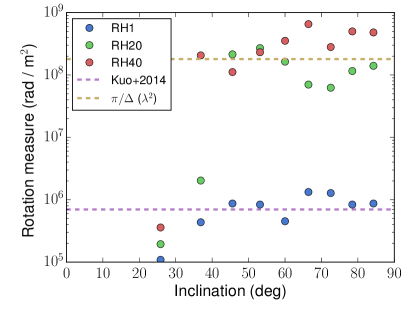
Figure 9: Faraday rotation measure as a function of viewing angle for disk (RH1) and jet (RH20, RH40) models. In all models, the RM increases with increasing inclination due to a growing accretion disk contribution. In the jet models, the disk is cold and dense, leading to RMs much larger than observed for $i\gtrsim 30^{\circ}$. In these cases, the RM quickly saturates near the maximum value we can resolve from our calculations with frequency spacing $\Delta\nu=1$ GHz centered on $230$ GHz, $\pi/(\lambda_{1}^{2}-\lambda_{2}^{2})\simeq 2\times 10^{8}\hskip 2.0pt\rm rad\hskip 2.0pt\rm m^{-2}$.

5 Summary

Disk+jet models of the M87* based on GRMHD simulations (Mościbrodzka et al., 2016) produce submillimetre images which are dominated either by the disk (low $\dot{M}$, hot disk electrons) or the counter-jet (high $\dot{M}$, cold disk electrons). The jet dominated models are consistent with the observed radio spectrum and jet morphologies. At short wavelengths the counter-jet produces the emission due to strong light bending effects (as first shown in Dexter et al. 2012). The cold accretion disk in these models Faraday depolarizes the counter-jet.

We find that in the majority of models Faraday rotation in the cold accretion disk depolarizes the counter-jet emission. The small residual polarization comes mostly from the forward jet and does not pass through the accretion disk, so that the observed Faraday rotation measure (RM) may be smaller than anticipated for a given mass accretion rate and using simple models. All models considered, even with accretion rates a factor $\simeq 10$ larger than the limit from Kuo et al. (2014), are still consistent with the measured RM of the M87*. It is possible that viable models could have even higher accretion rates than considered here ($\dot{M}>9\times 10^{-3}\,\rm M_{\odot}yr^{-1}$).

It is difficult to integrate the equations of polarized transfer with high accuracy in models with high Faraday depth. The inaccuracy is probably due to spacing of the geodesic points concentrated close to the black hole event horizon in the current scheme (and in most of similar types of codes). While this is convenient to produce accurate intensity images a lot of Faraday rotation (or conversion) can occur far from the black hole where the integration is not spaced well. This should be addressed by future radiative transfer models.

We examined a specific type of GRMHD simulations (so called standard and normal evolution models, SANEs). There are other possible models for the M87* (e.g. Magnetically Arrested Disks, McKinney et al. 2012), which we have not explored further. It should be feasible to check how RM depends on, e.g., mass accretion rate in these other models to find out if they are consistent with observations. In any case, our models predict different levels of polarization degree and possibly different Faraday rotation compared to semi-analytical models of the jet launching zone as presented in Broderick & Loeb (2009).

What are the implications of our results for other low luminosity supermassive black hole systems? Based on variability timescales analysis Bower et al. (2015) and spectral modelling Falcke (1996) the millimetre emission from the core of M81 (M81*) should also be coming from the immediate vicinity of the black hole event horizon (i.e., $\tau_{\rm abs}\leq 1$ at mm wavelengths). The Faraday rotation depth dependency on the mass of the black hole $M_{\rm BH}$ is $\tau_{\rm FR}\propto\dot{M}^{3/2}M_{\rm BH}^{-2}R_{\rm high}^{2}$ (because $n_{e}\propto\dot{M}/M_{\rm BH}^{2}$ and $B\propto\dot{M}^{1/2}/M_{\rm BH}$ but $dl\propto M_{\rm BH}$). Combining the above expression with numerical values of $\tau_{\rm FR}$ presented in Figure 1 we obtain an approximate general expression for the Faraday depth as a function of black hole mass, accretion rate, and proton-to-electron temperature ratio in the disk:

$$\tau_{\rm FR}\approx 1(\frac{\dot{M}}{10^{-4}\rm M_{\odot}yr^{-1}})^{3/2}(\frac{M_{\rm BH}}{6.2\times 10^{9}\mathrm{M}_{\odot}})^{-2}(R_{\rm high})^{2}.$$ (5)

Assuming that the mass of the supermassive black hole in M81* is $M_{\rm BH}=7\times 10^{7}M_{\odot}$ and, e.g., $R_{\rm high}=10$ we find that $\tau_{\rm FR}\gg 1$ for accretion rates $\dot{M}>10^{-7}\,\rm M_{\odot}yr^{-1}$. Hence, we conclude that it is likely that the effects presented in this work also will be visible in M81*, i.e., the millimetre source polarization will be scrambled and depolarized.

Appendix A Polarized radiative transfer in spherical coordinates

The non-relativistic polarised radiative transfer equation can be written in the form,

$$\frac{d}{ds}\left(\begin{array}[]{c}I\\ Q\\ U\\ V\\ \end{array}\right)=\left(\begin{array}[]{c}j_{I}\\ j_{Q}\\ j_{U}\\ j_{V}\end{array}\right)-\left(\begin{array}[]{cccc}\alpha_{I}&\alpha_{Q}&\alpha_{U}&\alpha_{V}\\ \alpha_{Q}&\alpha_{I}&\rho_{V}&\rho_{U}\\ \alpha_{U}&-\rho_{V}&\alpha_{I}&\rho_{Q}\\ \alpha_{V}&-\rho_{U}&-\rho_{Q}&\alpha_{I}\\ \end{array}\right)\left(\begin{array}[]{c}I\\ Q\\ U\\ V\\ \end{array}\right)$$ (6)

where ($I$, $Q$, $U$, $V$) are the Stokes parameters, $j_{I,Q,U,V}$ are the polarised emissivities, $\alpha_{I,Q,U,V}$ are the absorption coefficients, and $\rho_{Q,U,V}$ are the Faraday rotation and conversion coefficients.

In the absence of emission and absorption, the Faraday rotation coefficient $\rho_{V}$ produces oscillations in $Q$ and $U$, corresponding to a rotation of the polarization angle. As described in the text, numerical solutions to the equations as written above break down when the oscillation length is shorter than the radiative transfer grid spacing $\Delta s$. In this limit, we follow Shcherbakov et al. (2012) and transform the polarized Stokes parameters to “spherical” coordinates:

$$\left(\begin{array}[]{c}Q\\ U\\ V\\ \end{array}\right)=\left(\begin{array}[]{c}R_{S}\sin{\psi_{S}}\cos{\phi_{S}}\\ R_{S}\sin{\psi_{S}}\sin{\phi_{S}}\\ R_{S}\cos{\psi_{S}}\end{array}\right),$$ (7)

where $R_{S}^{2}=Q^{2}+U^{2}+V^{2}$ is the polarized intensity and $\phi_{S}$ and $\psi_{S}$ are angular Stokes parameters describing the linear polarization direction ($\phi_{S}$) and the relative amount of circular polarization ($\psi_{S}$). In terms of these spherical Stokes parameters, the transfer equations become:

$$\frac{dR_{S}}{ds} = \sin{\psi_{S}}\left[\cos{\phi_{S}}\left(j_{Q}-\alpha_{Q}I\right)+\sin{\phi_{S}}\left(j_{U}-\alpha_{U}I\right)\right]+\cos{\psi_{S}}\left(j_{V}-\alpha_{V}I\right)-\alpha_{I}R_{S},$$ (8)

$$\frac{d\phi_{S}}{ds} = \frac{\csc{\psi_{S}}}{R_{S}}\left[\cos{\phi_{S}}\left(j_{U}-\alpha_{U}I\right)-\sin{\phi_{S}}\left(j_{Q}-\alpha_{Q}I\right)\right]-\cot{\psi_{S}}\left(\cos{\phi_{S}}\rho_{Q}+\sin{\phi_{S}}\rho_{U}\right)+\rho_{V},$$ (9)

$$\frac{d\psi_{S}}{ds} = \frac{1}{R_{S}}\left\{\cos{\psi_{S}}\left[\cos{\phi_{S}}\left(j_{Q}-\alpha_{Q}I\right)+\sin{\phi_{S}}\left(j_{U}-\alpha_{U}I\right)\right]-\sin{\psi_{S}}\left(j_{V}-\alpha_{V}I\right)\right\}+\cos{\phi_{S}}\rho_{U}-\sin{\phi_{S}}\rho_{Q}.$$ (10)

In this form, the transfer equations are non-linear and must be solved by numerical integration. On the other hand, the Faraday effects now only appear in equations for the angular Stokes parameters, and so do not directly change the total polarized intensity, $R_{S}$. Further, these effects are now source terms, independent of the spherical Stokes parameters. When they change rapidly (e.g. $\Delta\phi_{S}\gg 2\pi$) during a single radiative transfer step, the accuracy in the solutions for the polarization angle and relative linear/circular polarization decreases. The total intensity and polarization fraction remain unchanged, however, allowing the integration to proceed even if the resulting Stokes $Q$, $U$, and $V$ are noisy (Table 1).

References

- Anderson et al. (2015) Anderson C. S., Gaensler B. M., Feain I. J., Franzen T. M. O., 2015, ApJ, 815, 49
- Beckert & Falcke (2002) Beckert T., Falcke H., 2002, A&A, 388, 1106
- Biretta et al. (1999) Biretta J. A., Sparks W. B., Macchetto F., 1999, ApJ, 520, 621
- Bower et al. (1999) Bower G. C., Wright M. C. H., Backer D. C., Falcke H., 1999, ApJ, 527, 851
- Bower et al. (2003) Bower G. C., Wright M. C. H., Falcke H., Backer D. C., 2003, ApJ, 588, 331
- Bower et al. (2015) Bower G. C., Dexter J., Markoff S., Gurwell M. A., Rao R., McHardy I., 2015, ApJ, 811, L6
- Broderick & Loeb (2009) Broderick A. E., Loeb A., 2009, ApJ, 697, 1164
- Broderick & McKinney (2010) Broderick A. E., McKinney J. C., 2010, ApJ, 725, 750
- Dexter (2016) Dexter J., 2016, MNRAS, 462, 115
- Dexter & Agol (2009) Dexter J., Agol E., 2009, ApJ, 696, 1616
- Dexter et al. (2012) Dexter J., McKinney J. C., Agol E., 2012, MNRAS, 421, 1517
- Doeleman et al. (2008) Doeleman S. S., et al., 2008, Nature, 455, 78
- Doeleman et al. (2012) Doeleman S. S., et al., 2012, Science, 338, 355
- Eatough et al. (2013) Eatough R. P., et al., 2013, Nature, 501, 391
- Falcke (1996) Falcke H., 1996, ApJ, 464, L67
- Feain et al. (2009) Feain I. J., et al., 2009, ApJ, 707, 114
- Feng et al. (2016) Feng J., Wu Q., Lu R.-S., 2016, ApJ, 830, 6
- Feretti et al. (2012) Feretti L., Giovannini G., Govoni F., Murgia M., 2012, A&ARv, 20, 54
- Gardner & Whiteoak (1966) Gardner F. F., Whiteoak J. B., 1966, ARA&A, 4, 245
- Gold et al. (2016) Gold R., McKinney J. C., Johnson M. D., Doeleman S. S., 2016, preprint, (arXiv:1601.05550)
- Haverkorn & Spangler (2014) Haverkorn M., Spangler S. R., 2014, Plasma Diagnostics of the Interstellar Medium with Radio Astronomy. p. 407, doi:10.1007/978-1-4899-7413-6_16
- Hindmarsh (1983) Hindmarsh A. C., 1983, in R. S. Stepleman et al. ed., Scientific Computing. pp 55–64 (arXiv:astro-ph/0402101)
- Jones & Odell (1977) Jones T. W., Odell S. L., 1977, ApJ, 214, 522
- Kuo et al. (2014) Kuo C. Y., et al., 2014, ApJ, 783, L33
- Li et al. (2016) Li Y.-P., Yuan F., Xie F.-G., 2016, preprint, (arXiv:1606.06029)
- Marrone (2006) Marrone D. P., 2006, PhD thesis, Harvard University
- Marrone et al. (2007) Marrone D. P., Moran J. M., Zhao J.-H., Rao R., 2007, ApJ, 654, L57
- Martí-Vidal et al. (2015) Martí-Vidal I., Muller S., Vlemmings W., Horellou C., Aalto S., 2015, Science, 348, 311
- McKinney et al. (2012) McKinney J. C., Tchekhovskoy A., Blandford R. D., 2012, MNRAS, 423, 3083
- Mertens et al. (2016) Mertens F., Lobanov A. P., Walker R. C., Hardee P. E., 2016, A&A, 595, A54
- Mościbrodzka et al. (2016) Mościbrodzka M., Falcke H., Shiokawa H., 2016, A&A, 586, A38
- Narayan et al. (1998) Narayan R., Mahadevan R., Grindlay J. E., Popham R. G., Gammie C., 1998, ApJ, 492, 554
- Pandya et al. (2016) Pandya A., Zhang Z., Chandra M., Gammie C. F., 2016, ApJ, 822, 34
- Plambeck et al. (2014) Plambeck R. L., et al., 2014, ApJ, 797, 66
- Shcherbakov (2008) Shcherbakov R. V., 2008, ApJ, 688, 695
- Shcherbakov et al. (2012) Shcherbakov R. V., Penna R. F., McKinney J. C., 2012, ApJ, 755, 133