General form of DMPK equation

1. Introduction

The Dorokhov–Mello–Pereyra–Kumar (DMPK) equation [1, 2, 3, 4] is an efficient instrument for investigation of quasi-1D disordered systems (see the paper [5] for a review). It describes evolution of diagonal elements of the many-channel transfer matrix due to increasing the system length. The DMPK equation is obtained from the maximum entropy principle (assuming the maximal randomness consistent with the symmetry restrictions) and conceptually close to the random matrix theory by Wigner and Dyson [6]. It is determined by one parameter (the system size in units of the correlation length) and manifests universality specific for the metallic state. The DMPK equation is equivalent to the super-symmetric sigma-model [7], derived from the microscopic Hamiltonians [8, 9, 10], but allows to work with distributions of physical quantities. Solution of the DMPK equation [3, 4] reproduces the universal fluctuations of conductance and quantum corrections to it obtained from diagrammatic calculations [11, 12].

In principle, the transfer matrix approach underlining the DMPK equation is not restricted by the quasi-1D geometry. Considering a system of $N$ coupled one-dimensional chains and arranging the chains in accordance with symmetry of a $d$-dimensional lattice, one can construct the systems of higher dimensionality. However, assumptions underlining the DMPK equation lead to statistical equivalence of chains and eliminate all information on the topology of space in the transverse directions. As a result, the DMPK equation cannot be used for study of the Anderson transition and is restricted by the metallic phase in the corresponding $d$-dimensional space. In the localized regime of a $d$-dimensional system, the DMPK equation is not adequate even for the quasi-1D geometry: it predicts the minimal Lyapunov exponent to be of order $1/N$, while the reasonable microscopic models lead to the result $O(1)$ [13, 14]. The latter can be understood easily in the regime of strong localization, when conductance is determined by one resonant trajectory and the system in fact becomes strictly one-dimensional .

It should be clear that in the general case assumptions used in the DMPK equation should be relaxed; in particular, it is necessary for describing universality arising near the Anderson transition. Derivation of the most general form of the DMPK equation is a problem, realized by scientific community [3, 4, 14, 16] and admitted to be of fundamental significance. One of the possible generalizations was suggested by Muttalib and co-workers [16]–[18].

We show below that the equation of the DMPK type may be derived under minimal assumptions on the properties of channels. Generally, this equation is of the diffusion type with a tensor character of the diffusion coefficient and finite values of non-diagonal components. We consider three different forms of the diagonal approximation, one of which reproduces the usual DMPK equation and its generalization suggested in [16]–[18]. Two other variants lead to equations of the same structure, but with different definition of their parameters. They contain the additional term, which is absent in the first variant and turned out to be very actual in the recent research of the conductance distribution [15].

2. Main concepts

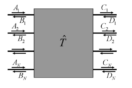
Figure 1: The many-channel transfer matrix $\hat{T}$ relates the amplitudes of the plane waves on the left ($A_{n}$, $B_{n}$) and on the right ($C_{n}$, $D_{n}$) of a scatterer.

Considering the system as a set of $N$ coupled one-dimensional chains, we can thought of it as a ”black box” with attached ideal contacts in the form of isolated $1D$ conductors . Then the system can be treated as an effective scatterer and described by the transfer matrix $\hat{T}$, relating the amplitudes of waves on the left ($A_{n}e^{ikx}+B_{n}e^{-ikx}$ in $n$-th channel) and on the right ($C_{n}e^{ikx}+D_{n}e^{-ikx}$) of the scatterer (Fig.1):

$$\left(\begin{array}[]{cc}A\\ B\end{array}\right)\,=\hat{T}\left(\begin{array}[]{cc}C\\ D\end{array}\right)\,=\left(\begin{array}[]{cc}T_{11}&T_{12}\\ T_{21}&T_{22}\end{array}\right)\,\left(\begin{array}[]{cc}C\\ D\end{array}\right)\,,$$

where $A$, $B$, $C$, $D$ are vectors with components $A_{n}$, $B_{n}$, $C_{n}$, $D_{n}$. In the vector notation, the form of Eq. 1 does not depend on the number of channels, while the transfer matrix is divided naturally into four blocks; it allows a parametrization [3, 20]

$$\hat{T}=\left(\begin{array}[]{cc}u_{1}&0\\ 0&v_{1}\end{array}\right)\,\left(\begin{array}[]{cc}\sqrt{1+\lambda}&\sqrt{\lambda}\\ \sqrt{\lambda}&\sqrt{1+\lambda}\end{array}\right)\,\left(\begin{array}[]{cc}u&0\\ 0&v\end{array}\right)\,,$$

where $u$, $v$, $u_{1}$, $v_{1}$ are unitary matrices, and $\lambda$ is a diagonal matrix with the positive elements $\lambda_{i}$, which are eigenvalues of the Hermitian matrix $T_{12}T^{+}_{12}$. In the presence of time reversal invariance the additional relations arise [2, 3]

$$v=u^{*}\,,\qquad v_{1}=u_{1}^{*}\,,$$

which as a rule are of no significance for the following.

Of the main interest are parameters $\lambda_{i}$, which in particular determine the conductance

$$g=\sum\limits_{i}\frac{1}{1+\lambda_{i}}\,$$

(in the Economou–Soukoulis definition [21, 22]). The DMPK equation describes evolution of their mutual distribution function $P\left(\lambda_{1},\lambda_{2},\ldots,\lambda_{N}\right)\equiv P\{\lambda\}$ with increasing the length $L$ of the system

$$\frac{\partial P\{\lambda\}}{\partial L}=\alpha\,\sum\limits_{i}\frac{\partial}{\partial\lambda_{i}}\left[\,\lambda_{i}(1+\lambda_{i})\,J\{\lambda\}\frac{\partial}{\partial\lambda_{i}}\,\frac{P\{\lambda\}}{J\{\lambda\}}\,\right]$$

$$J\{\lambda\}=\prod\limits_{i<j}|\lambda_{i}-\lambda_{j}|^{\beta}\,,$$

where $\beta=1$ for the orthogonal ensemble (usual systems with a random potential), $\beta=2$ for the unitary ensemble (systems in the strong magnetic field), $\beta=4$ for the symplectic ensemble (system with the strong spin-orbit interaction); parameter $\alpha$ has a sense of the inverse correlation length of the quasi-1D system. The quantity $J\{\lambda\}$ is well-known from the random matrix theory [6] and arises from the Jacobian of transformation

$$\prod\limits_{ij}dH_{ij}=J\{\lambda\}\,\tilde{J}\{Q\}\,\prod\limits_{i}d\lambda_{i}\prod\limits_{ij}dQ_{ij}$$

when integration over elements of the matrix $\hat{H}$ is replaced by integration over its eigenvalues $\lambda_{i}$ and the elements of diagonalizing matrix $\hat{Q}$ ($\hat{H}=\hat{Q}^{-1}\hat{\Lambda}\hat{Q}$). In fact, $J\{\lambda\}$ is the distribution function of levels, if they are contained in the restricted interval with the periodic boundary conditions (the Dyson circular ensemble). In actual applications, the distribution $P\{\lambda\}$ includes the additional factor, providing localization of the spectrum in a finite interval and practically not affecting the distribution of close levels. Analogously, the distribution $P\{\lambda\}=J\{\lambda\}$ is a formal solution of equation (5) but does not satisfy the normalization condition; an additional factor becomes inevitable, whose evolution is described by the DMPK equation. Exact solution of Eq.5 for $\beta=2$ shows [23] that the additional factor is not reduced to a smooth envelope but essentially changes the distribution $P\{\lambda\}$, making it different from $J\{\lambda\}$ even on the local level; correlations of $\lambda_{i}$ are determined by the Jacobian $J\{\lambda\}$ only at the initial stage of evolution, when all $\lambda_{i}$ are small. In the context of generalizations of the DMPK equation this circumstance acquires a deep sense (see Footnote 9 in Sec. 5).

In a strictly one-dimensional system we have $J\{\lambda\}=1$ and equation (5) reduces to the form

$$\frac{\partial P(\lambda)}{\partial L}=\alpha\,\frac{\partial}{\partial\lambda}\left[\,\lambda(1+\lambda)\,\frac{\partial P(\lambda)}{\partial\lambda}\,\right]\,,$$

and $\lambda$ coincides with the Landauer resistance $\rho$ [24]; such equation was derived in many papers [25]–[29]. Recently it was shown by the present author [15] that the general evolution equation in 1D systems has a form

$$\frac{\partial P(\lambda)}{\partial L}=\alpha\,\frac{\partial}{\partial\lambda}\left[-\gamma(1+2\lambda)P(\lambda)+\lambda(1+\lambda)\frac{\partial P(\lambda)}{\partial\lambda}\,\right],$$

and the additional term, specified by parameter $\gamma$, is physically significant: its incorporation in the Shapiro scheme [30] allows to explain all essential features in the conductance distribution, which was impossible on the basis of (7). This term disappears in the random phase approximation and is naturally not reproduced by equation (5), based on the analogous assumptions. However, this term is also not predicted by the generalized DMPK equation suggested by Muttalib and co-workers [16]–[18]

$$\frac{\partial P\{\lambda\}}{\partial L}=\alpha\sum\limits_{i}K_{ii}\frac{\partial}{\partial\lambda_{i}}\left[\,\lambda_{i}(1+\lambda_{i})\,J_{i}\{\lambda\}\frac{\partial}{\partial\lambda_{i}}\,\frac{P\{\lambda\}}{J_{i}\{\lambda\}}\,\right]$$

$$J_{i}\{\lambda\}=\prod\limits_{j<k}|\lambda_{j}-\lambda_{k}|^{\beta^{i}_{jk}}\,,\qquad\beta^{i}_{jk}=2K_{jk}/K_{ii}$$

and containing as parameters the elements $K_{ij}$ of a certain matrix $\hat{K}$.  This fact clearly demonstrates that attempts of generalization of the DMPK equation are not sufficiently advanced and do not reproduce all essential contributions. This point was the main motivation of the present paper.

3. Idea of derivation

Derivation of the evolution equation is based on the relation

$$\hat{T}_{L+\Delta L}=\hat{T}_{L}\,\hat{T}_{\Delta L}\,,$$

where $\hat{T}_{\Delta L}$ is a matrix close to the unit one. The form of the DMPK equation depends on statistical properties of the parameters $\epsilon_{k}$, determining deviations of $\hat{T}_{\Delta L}$ from the unit matrix. These parameters can be divided into two groups: for the first of them

$$\langle\epsilon_{k}\rangle\neq 0\,,$$

while for the second

$$\langle\epsilon_{k}\rangle=0\,,\qquad\langle\epsilon^{2}_{k}\rangle\neq 0\,.$$

The presence of parameters (12) is necessary for arising of an equation of the diffusion type: since there is no effect in the first order in $\epsilon_{k}$, all calculations should be made in the second order, and this is a reason for appearing of the second derivatives which are characteristic for the diffusion equation. The general strategy consists in averaging only over parameters (12), and making no assumptions relative to parameters (11).

To obtain the most general form of the DMPK equation, we should distinguish the category of quantities, for which the property (12) is not a model assumption but is an inherent property, following from their nature. Such quantities are well known and related with a diagonal disorder. Consider the Schroedinger equation with a random potential, which is defined on the lattice sites by a set of independent random quantities $V_{n}$ (as in the Anderson model). Variables $V_{n}$ should have identical distributions to provide a spatial homogeneity in average. If the mean value $\langle V_{n}\rangle$ is finite, then it is equal for all $n$ and can be excluded by a shift of the origin of energy $E$, since a random potential enters in the combination $V_{n}-E$. Thus, we can accept without a loss of generality

$$\langle V_{n}\rangle=0\,,\qquad\langle V^{2}_{n}\rangle=W^{2}\,,$$

as it is made in almost all theoretical papers.

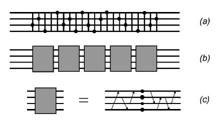
Figure 2: (a) A typical quasi-1D system is a bar, cutout of the $d$-dimensional lattice, with randomly located impurities inserted in it. (b) The system can be divided into a sequence of effective scatterers, whose transfer matrices are multiplied. (c) Each scatterer provides a partial reflection of the incident waves and mixing of channels; these two processes can be imagined as somewhat separated in space.

This point can be used in the following manner. A typical quasi-1D system is a bar cutout of a $d$-dimensional lattice and containing randomly located impurities (Fig. 2,a). We can divide it into a series of effective scatterers containing a lot of lattice sites (Fig. 2,b). Each scatterer should provide existence of two effects, (a) a partial reflection of the incident waves, and (b) mixing of channels. It is convenient to imagine these two processes as slightly separated in space (Fig. 2,c), so that there is a region where waves are reflected without mixing of channels, and there are two regions where channels are mixed for the transmitted and back-scattered waves but no reflection occurs. Such assumption is not very essential, since we suppose nothing on the degree of separation and it can be purely symbolic. In fact, the construction in Fig. 2,c corresponds to the canonical representation (2) of the transfer matrix: it is easy to see that the middle matrix in (2) provides a reflection of waves without mixing of channels, while the right and the left matrices provide mixing of channels without reflection of waves.

The middle part of the effective scatterer (Fig. 2,c) can be described by the transfer matrix

$$\left(\begin{array}[]{cc}1-i\epsilon&-i\epsilon\\ i\epsilon&1+i\epsilon\end{array}\right)\,,$$

corresponding to the diagonal disorder created by point scatterers on the independent one-dimensional chains, so $\epsilon$ is a diagonal matrix with real elements $\epsilon_{k}$, possessing the property (12). Extracting from (14) the factors, not related with scattering, we can accept the following representation for matrix $\hat{T}_{\Delta L}$

$$\hat{T}_{\Delta L}=\left(\begin{array}[]{cc}\!\!w_{1}\!&\!0\!\!\\ \!\!0\!&\!w_{2}\!\!\end{array}\right)\,\left(\begin{array}[]{cc}\!\!\sqrt{1+\epsilon^{2}}&-i\epsilon\\ i\epsilon&\!\sqrt{1+\epsilon^{2}}\!\!\end{array}\right)\,\left(\begin{array}[]{cc}\!\!w_{3}\!&\!0\!\!\\ \!\!0\!&\!w_{4}\!\!\end{array}\right),$$

where $w_{1}$, $w_{2}$, $w_{3}$, $w_{4}$ are matrices close to the unit one and elements $\epsilon_{k}$ are small. Accepting the canonical representation (2) for $\hat{T}_{L}$ and composing the product (10), one can see that matrices $w_{1}$, $w_{2}$ lead to a small renormalization of matrices $u$ and $v$, which can be neglected . It is clear that we should compose the product

$$\hat{T}^{\prime}=\left(\begin{array}[]{cc}\sqrt{1+\lambda}&\sqrt{\lambda}\\ \sqrt{\lambda}&\sqrt{1+\lambda}\end{array}\right)\,\left(\begin{array}[]{cc}u&0\\ 0&v\end{array}\right)\,\cdot\qquad$$

$$\qquad\qquad\qquad\cdot\,\left(\begin{array}[]{cc}\sqrt{1+\epsilon^{2}}&-i\epsilon\\ i\epsilon&\sqrt{1+\epsilon^{2}}\end{array}\right)\,$$

and reduce it to the canonical form (2).

The assumption of a diagonal disorder for the middle part of an effective scatterer (Fig. 2,c) is not very essential. Indeed, the notion of weak scatterers is inevitable in derivation of the differential equation; in the opposite case only the finite difference equation is possible. Having in mind a description of the Anderson transition, we should work near the band edge of the ideal crystal, since only there a weak disorder is compatible with localization in higher dimensions. Then the de Broglie wavelength and the mean free path are large in comparison with the atomic spacing and the wave function envelope changes slowly. It allows to introduce the coarse description, dividing the system into blocks, small in comparison with the wavelength but containing a lot of the lattice sites, and considering these blocks as the new lattice sites. In the result of such procedure practically any short-ranged random potential reduces to the diagonal Gaussian disorder. Universality arising near the Anderson transition as in other critical phenomena [32, 33] leads to equivalence of its description near the band edge and in the band center.

4. General evolution equation

Let describe the general scheme of deriving the evolution equation, while the calculation details can be found in Appendix $A$. Parameters $\lambda^{\prime}_{i}$ of the matrix $\hat{T}^{\prime}$ can be found as eigenvalues of the Hermitian ”Hamiltonian” $H=T_{12}T^{+}_{12}$, where

$$T_{12}=\sqrt{1+\lambda}\,u\,(-i\epsilon)+\sqrt{\lambda}\,v\,\sqrt{1+\epsilon^{2}}\,,$$

and can be presented as functions of $\lambda_{i}$ ($\lambda^{\prime}_{i}=f_{i}\{\lambda\}$) in the form of expansion over $\epsilon$. Composing the distribution function of $\lambda^{\prime}_{i}$, we have

$$P_{L+\Delta L}\{\lambda^{\prime}\}=\int\prod\limits_{i}d\lambda_{i}P_{L}\{\lambda\}\prod\limits_{i}\delta\left(\lambda^{\prime}_{i}-f_{i}\{\lambda\}\right)\cdot$$

$$\cdot P(\epsilon)\,P(u,v)\,d\epsilon\,du\,dv\,.\,$$

Making a change of variables $y_{i}=f_{i}\{\lambda\}$, one can replace integration over $\lambda_{i}$ by integration over $y_{i}$

$$\prod\limits_{i}d\lambda_{i}=I\{y\}\prod\limits_{i}dy_{i}\,,$$

while the inverse relations $\lambda_{i}=g_{i}\{y\}$ are found by iterations in $\epsilon$. Integration over $y_{i}$ removes the $\delta$-functions and leads to the result

$$P_{L+\Delta L}\{\lambda\}=\int I\{\lambda\}P_{L}\{g_{i}\{\lambda\}\}P(\epsilon)P(u,v)\,d\epsilon\,du\,dv\,.$$

In calculation of the Jacobian $I\{y\}$ one discovers that its diagonal elements are of order unity, while non-diagonal elements are of order $\epsilon^{2}$, so in fact it reduces to the product of diagonal elements. Substituting for $I\{\lambda\}$ and $g_{i}\{\lambda\}$ their expansions in $\epsilon$ and expanding (20) to the second order, we produce averaging according to $\langle\epsilon_{k}\rangle=0$, $\langle\epsilon_{k}\epsilon_{k^{\prime}}\rangle=\langle\epsilon^{2}\rangle\,\delta_{kk^{\prime}}$ and set  $\langle\epsilon^{2}\rangle\equiv\alpha\Delta L$. As a result

$$\!\!\frac{\partial P\{\lambda\}}{\partial L}\!=\alpha\!\sum\limits_{i}\frac{\partial}{\partial\lambda_{i}}\!\left[G_{i}\{\lambda\}P\{\lambda\}\!+\!\sum\limits_{j}F_{i\!j}\{\lambda\}\frac{\partial P\{\lambda\}}{\partial\lambda_{j}}\,\!\right]$$

where the following functions of $\lambda_{i}$ are introduced (the primes near the summation signs indicate the absence of terms with $j=i$)

$$F_{ij}\{\lambda\}=\frac{1}{2}\sqrt{\lambda_{i}(1+\lambda_{i})\lambda_{j}(1+\lambda_{j})}\,A_{ij}\,,$$

$$G_{i}\{\lambda\}=(1+2\lambda_{i})\left(\frac{1}{2}A_{ii}-1\right)+\qquad$$

$$+\sqrt{\lambda_{i}(1+\lambda_{i})}\,{\sum\limits_{j}}^{\prime}\frac{1+2\lambda_{j}}{4\sqrt{\lambda_{j}(1+\lambda_{j})}}\,A_{ij}-\tilde{G}_{i}\{\lambda\}\,,$$

$$\tilde{G}_{i}\{\lambda\}={\sum\limits_{j}}^{\prime}\frac{\lambda_{i}(1+\lambda_{j})\,B_{ij}+\lambda_{j}(1+\lambda_{i})\,C_{ij}}{\lambda_{i}-\lambda_{j}}\,+$$

$$\qquad\qquad\qquad+{\sum\limits_{j}}^{\prime}\frac{\sqrt{\lambda_{i}(1+\lambda_{i})\lambda_{j}(1+\lambda_{j})}}{\lambda_{i}-\lambda_{j}}\,D_{ij}$$

with a definition of matrices

$$B_{ij}=\sum\limits_{k}\overline{|v_{ik}|^{2}|u_{jk}|^{2}}\,,\qquad C_{ij}=\sum\limits_{k}\overline{|u_{ik}|^{2}|v_{jk}|^{2}}\,,$$

$$D_{ij}=-\sum\limits_{k}\left(\overline{v_{ik}v_{jk}u^{*}_{ik}u^{*}_{jk}}+\overline{v^{*}_{ik}v^{*}_{jk}u_{ik}u_{jk}}\right)\,,$$

$$A_{ij}=\sum\limits_{k}\left(\overline{u_{ik}u^{*}_{jk}v^{*}_{ik}v_{jk}}+\overline{u^{*}_{ik}u_{jk}v_{ik}v^{*}_{jk}}-\right.$$

$$\qquad\quad\left.-\overline{u_{ik}u_{jk}v^{*}_{ik}v^{*}_{jk}}-\overline{u^{*}_{ik}u^{*}_{jk}v_{ik}v_{jk}}\right)\,.$$

Equation (21) is the most general form of the DMPK equation: in its derivation we did not use any assumptions on the statistical properties of matrices $u$ and $v$, and they even are not obliged to be random. The right hand side of (21) is a sum of full derivatives, which provides the conservation of the total probability.

5. Diagonal forms

Equation (21) is of the diffusion type, with a tensor character of the diffusion coefficient and finite non-diagonal components. In the general form it is rather complicated and hardly suitable for a constructive analysis; so consider its possible simplifications.

Equation (21) is simplified radically, if we assume the diagonal form for matrices $A_{ij}$ and $D_{ij}$

$$A_{ij}=A_{i}\delta_{ij}\,,\qquad D_{ij}=D_{i}\delta_{ij}\,.$$

We accept also $B_{ij}=C_{ij}\equiv K_{ij}$, since the statistical properties of matrices $u$ and $v$ are usually identical. Then equation (21) reduces to the form (see Appendix $B$)

$$\frac{\partial P\{\lambda\}}{\partial L}=\alpha\,\sum\limits_{i}\frac{1}{2}A_{i}\frac{\partial}{\partial\lambda_{i}}\left[\,-\gamma_{i}(1+2\lambda_{i})\,P\{\lambda\}+\phantom{\frac{P\{\lambda\}}{J_{i}\{\lambda\}}}\right.$$

$$\qquad\left.+\lambda_{i}(1+\lambda_{i})\,J_{i}\{\lambda\}\frac{\partial}{\partial\lambda_{i}}\,\frac{P\{\lambda\}}{J_{i}\{\lambda\}}\,\right]$$

$$\gamma_{i}=(2K_{ii}-A_{i})/A_{i}\,,\qquad$$

$$J_{i}\{\lambda\}=\prod\limits_{j<k}|\lambda_{j}-\lambda_{k}|^{\beta^{i}_{jk}}\,,\qquad\beta^{i}_{jk}=4K_{jk}/A_{i}\,,$$

which reproduces Eq. 8 in the one-channel case. Conditions for realization of the diagonal approximation can be easily analyzed for the unitary ensemble, when matrices $u$ and $v$ are averaged independently. If a unitary matrix $u$ is restricted by real values of its elements, then it turns into the orthogonal matrix $\tilde{u}$; to restore the unitary matrix we should add to the elements of $\tilde{u}$ the appropriate phase factors. Producing the same manipulations with the matrix $v$, we set

$$u_{lk}=\tilde{u}_{lk}e^{i\varphi_{lk}}\,,\qquad v_{lk}=\tilde{v}_{lk}e^{i\phi_{lk}}\,$$

and obtain after substitution to (23)

$$\!B_{ij}=\sum\limits_{k}\left\langle|\tilde{v}_{ik}|^{2}|\tilde{u}_{jk}|^{2}\right\rangle\,,\quad C_{ij}=\sum\limits_{k}\left\langle|\tilde{u}_{ik}|^{2}|\tilde{v}_{jk}|^{2}\right\rangle,$$

$$\!\!D_{ij}=\!-2\sum\limits_{k}\left\langle\tilde{v}_{ik}\tilde{v}_{jk}\tilde{u}_{ik}\tilde{u}_{jk}\cos(\phi_{ik}\!+\!\phi_{jk}\!-\!\varphi_{ik}\!-\!\varphi_{jk}\right)\rangle$$

$$\!\!A_{ij}=4\sum\limits_{k}\left\langle\tilde{v}_{ik}\tilde{v}_{jk}\tilde{u}_{ik}\tilde{u}_{jk}\sin(\varphi_{ik}\!-\!\phi_{ik})\sin(\varphi_{jk}\!-\!\phi_{jk}\right)\rangle$$

If matrices $\tilde{v}$ and $\tilde{u}$ are completely random, while phases $\varphi_{ik}$ and $\phi_{ik}$ have nonuniform distributions, then products $\tilde{v}_{ik}\tilde{v}_{jk}$, $\tilde{u}_{ik}\tilde{u}_{jk}$ are averaged to zero for $i\neq j$, providing the diagonal approximation (24) where $A_{i}$ and $K_{ij}$ are independent, and the trivial result is valid for $K_{ij}$ (see Eq. 28 below). Contrary, if matrices $\tilde{v}$ and $\tilde{u}$ are not sufficiently random, but phases $\varphi_{ik}$ and $\phi_{ik}$ are completely stochastic, then we have another diagonal approximation with nontrivial values of $K_{ij}$ and relation $A_{i}=2K_{ii}$; as a result, the terms with $\gamma_{i}$ turn to zero and Eq. 25 reduces to the variant (9), suggested by Muttalib et al [16]–[18]. Finally, if both $\tilde{v}$, $\tilde{u}$, and $\varphi_{ik}$, $\phi_{ik}$ are completely random, then averaging occurs over the unitary group (see Appendix $B$ in [5]) and leads to the results

$$K_{ij}=\sum\limits_{k}\left\langle|v_{ik}|^{2}\right\rangle\left\langle|u_{jk}|^{2}\right\rangle=\frac{1}{N}\qquad\mbox{\rm and}\quad\beta^{i}_{jk}=2\,,$$

$$K_{ij}=\sum\limits_{k}\left\langle|u_{ik}|^{2}|u_{jk}|^{2}\right\rangle=\frac{1+\delta_{ij}}{N+1}\,\quad\mbox{\rm and}\quad\beta^{i}_{jk}=1$$

for the unitary and the orthogonal ensembles correspondingly, so equation (9) transforms to the usual DMPK equation (5). 

Let us discuss the third variant of the diagonal approximation, which we consider as the most actual. It was argued in [15, 34], that for the correct definition of conductance of a finite system it is useful to introduce semi-transparent boundaries, separating the system from the ideal leads attached to it. In the limit of weak transparency one obtains universal equations, independent on the way how the contact resistance of the reservoir is excluded [35] (all formulas of the Landauer type [36]–[40] reduce in this limit to the variant by Economou–Soukoulis [21, 22]), which then can be extrapolated to transparency of order unity. Such definition is surely referred to the system under consideration (and not to the composed system ”sample+ideal leads”) and provides the infinite value of conductance for an ideal system [34].

Suppose that weakly-transparent boundaries are created by point scatterers inserted in one-dimensional chains attached to the system (Fig. 2,a); then its transfer matrix $\hat{T}$ transforms to $\hat{T}_{0}\hat{T}\hat{T}_{0}$, i.e.

$$\left(\begin{array}[]{cc}\!\!1\!-\!i\kappa&-i\kappa\\ i\kappa&1\!+\!i\kappa\!\!\end{array}\right)\left(\begin{array}[]{cc}T_{11}&T_{12}\!\\ T_{21}&T_{22}\!\end{array}\right)\left(\begin{array}[]{cc}\!\!1\!-\!i\kappa&-i\kappa\\ i\kappa&1\!+\!i\kappa\!\!\end{array}\right),$$

where $\kappa$ is a diagonal matrix. Reducing (30) to the canonical form (2), one has in the main approximation for large $\kappa$

$$u_{1}\sqrt{1+\lambda}\,u=-\kappa\tilde{T}\kappa\,,$$

$$u_{1}\sqrt{\lambda}\,v=-\kappa\tilde{T}\kappa\,,$$

$$v_{1}\sqrt{\lambda}\,u=\kappa\tilde{T}\kappa\,,$$

$$v_{1}\sqrt{1+\lambda}\,v=\kappa\tilde{T}\kappa\,,$$

where $\tilde{T}=T_{11}-T_{12}+T_{21}-T_{22}$. Since the unitary matrices $u$, $v$, $u_{1}$, $v_{1}$ have restricted elements, then $\lambda\sim\kappa^{4}$ and $1+\lambda$ can be replaced by $\lambda$; then (31) gives

$$u=v,\quad u_{1}=-v_{1}\,\quad\mbox{\rm for}\,\quad\kappa\to\infty\,.$$

For large $\lambda_{i}$ equations (21–23) reduce to the form analogous to (25), but with another definition of $K_{ij}$ (see Appendix $B$), $K_{ij}=(B_{ij}+C_{ij}+D_{ij})/2$. Substitution of (32) into (23) gives $K_{ij}\to 0$, $A_{ij}\to 0$ in the $\kappa\to\infty$ limit. For large, but finite $\kappa$ the small deviations of $v$ from $u$ should be taken into account, setting

$$v=ue^{ih}\,,$$

where $h$ is the Hermitian matrix with small elements. Substituting (33) into (23) and expanding to the second order in $h$, one has

$$2K_{ij}=\sum\limits_{k}\left\langle|u_{ik}|^{2}|u_{jk}|^{2}\left(|h_{ik}|^{2}+|h_{jk}|^{2}+\right.\right.\qquad\qquad\qquad$$

$$\qquad\qquad\qquad\qquad+\left.\left.h_{ik}h_{jk}+h^{*}_{ik}h^{*}_{jk}\right)\right\rangle\,,$$

$$A_{ij}=\sum\limits_{k}\left\langle|u_{ik}|^{2}|u_{jk}|^{2}\left(h_{ik}h_{jk}+h^{*}_{ik}h^{*}_{jk}+\right.\right.\qquad\qquad$$

$$\qquad\qquad\qquad\qquad+\left.\left.h^{*}_{ik}h_{jk}+h_{ik}h^{*}_{jk}\right)\right\rangle\,.$$

It is easy to see, that $A_{ii}=2K_{ii}$ independently of the $h_{ik}$ statistics (in fact, it follows from the general expressions (23)). For large $\kappa$, the quantities $h_{ik}$ are small in magnitude, but there are no other restrictions on their statistics. It is natural to think that $h_{ik}$ fluctuate randomly and their fluctuations are independent of $u_{ik}$.  Then pair products $h_{ik}h_{jk}$, $h^{*}_{ik}h_{jk}$, $\ldots$ with $i\neq j$ are averaged to zero, and the matrix $A_{ij}$ becomes diagonal. As a result, equation (21) accepts the form

$$\frac{\partial P\{\lambda\}}{\partial L}=\alpha\,\sum\limits_{i}K_{ii}\frac{\partial}{\partial\lambda_{i}}\left[\,-\gamma_{i}(1+2\lambda_{i})\,P\{\lambda\}+\phantom{\frac{P\{\lambda\}}{J_{i}\{\lambda\}}}\right.$$

$$\left.+\lambda_{i}(1+\lambda_{i})\,J_{i}\{\lambda\}\frac{\partial}{\partial\lambda_{i}}\,\frac{P\{\lambda\}}{J_{i}\{\lambda\}}\,\right]$$

$$J_{i}\{\lambda\}=\prod\limits_{j<k}|\lambda_{j}-\lambda_{k}|^{\beta^{i}_{jk}}\,,\qquad\beta^{i}_{jk}=2K_{jk}/K_{ii}$$

$$\gamma_{i}=(1-\sum_{j}K_{ij})/K_{ii}\,,\qquad K_{ij}=(B_{ij}+C_{ij}+D_{ij})/2\,$$

and has the same structure as (25), but with different definition of parameters. Since $K_{ij}$ are small for large $\kappa$, parameters $\gamma_{i}$ are surely finite and large in magnitude.

The first two diagonal approximations look somewhat artificial. If matrices $u$ and $v$ are completely random, then we return to the initial equation (5). If $u$ and $v$ are not sufficiently random, then a tendency to the non-diagonal situation arises: we do not see serious grounds why $\tilde{u}_{ij}$ should be more random than $\varphi_{ij}$ or vice versa. Contrary, the third variant of a diagonal approximation looks quite natural: existence of weakly transparent boundaries restricts mutual fluctuations of $u$ and $v$, but beyond these restrictions they are considered as completely random. Simultaneously, all situation with the definition of conductance becomes logically consistent.

It is well-known [2, 5], that equation (5) is easily solved in the limit of large $L$, when parameters $\lambda_{i}$ are large and obey hierarchy $\lambda_{1}\gg\lambda_{2}\gg\ldots\gg\lambda_{N}$; then $J\{\lambda\}$ reduces to the product of powers of $\lambda_{i}$ and equation (5) splits into $N$ independent equations. Applying the same procedure to equation (35), we find the independent Gaussian distributions for quantities $x_{i}=\ln\lambda_{i}$ defined by their first two moments:

$$\langle x_{i}\rangle=\alpha L\left[(2\gamma_{i}+1)K_{ii}+2\sum\limits^{N}_{j=i+1}K_{ij}\right]\,,\qquad$$

$$\sigma^{2}_{i}=\langle x_{i}^{2}\rangle-\langle x_{i}\rangle^{2}=2\alpha L\,K_{ii}\,,$$

which for $\gamma_{i}=0$ coincides with results of [14, 17]. In the approximation of equivalent channels one can set $\alpha K_{ii}=\tilde{\alpha}$, $\beta_{ij}=\beta$, $\gamma_{i}=\gamma$, and equation (35) is determined by three parameters $\tilde{\alpha}L$, $\beta$, $\gamma$; in particular,

$$\frac{2\langle x_{i}\rangle}{\sigma^{2}_{i}}=2\gamma+1+\beta(N-i)$$

and parameters $\beta$, $\gamma$ can be easily estimated from numerical data on Lyapunov exponents (see e.g. [41, 42]). One can see from formula (32) of the paper [42] that relation $\sigma^{2}_{i}=2\langle x_{i}\rangle$ for the minimal exponent ($i=N$ in our notation) is valid in the metallic regime but violated in other cases; hence the parameter $\gamma$ is finite beyond the metallic phase. 

As clear from derivation, the structure of equation (35) is the same for the unitary and orthogonal ensembles; correspondingly, $\beta$ becomes a free parameter not related with the Wigner–Dyson values, and in the general case transforms to a matrix . It is clear that the ”pure” Wigner–Dyson ensembles loose their actuality beyond the metallic phase, and in particular are not adequate for description of the Anderson transition. The latter circumstance is not accounted for in the existent versions of the sigma-models [8, 9, 10], which are equivalent to the simplest equation (5) and require modification for incorporation of the discussed generalizations. The only exclusion is the situation for $d=2+\epsilon$, where universality arising near the critical point approximately corresponds to universality specific for the metallic phase, which is adequately described by equation (5). It provides validity of results in the main $\epsilon$-approximation but remains the open question on their validity in higher orders.

6. Conclusion

In the present paper we derive the DMPK equation under minimal assumptions on the properties of channels. It is of the diffusion type with a tensor character of the diffusion coefficient and nonzero off-diagonal components. We suggest three variants of the diagonal approximation, one of which reproduces the usual DMPK equation and its generalization suggested in [16]–[18]. Two other variants lead to equations of the same structure and contain additional terms specified by parameters $\gamma_{i}$.

The most general form of the DMPK equation, given by Eq. 21, probably is not very actual: it should be used as a starting point for new statistical hypotheses, which were adequate for description of the Anderson transition. The methods used in numerical experiments allow to calculate matrices $u$ and $v$ [19], and analyzing their statistical properties establish the form of matrices $A_{ij}$, $B_{ij}$, $C_{ij}$, $D_{ij}$. Numerical analysis undertaken in the context of equation (9) [18, 31] , points out the realization of the diagonal approximation and deviation of parameters $\beta^{i}_{jk}$ from their Wigner–Dyson values; a finiteness of parameters $\gamma_{i}$ follows from Eq.32 of [42]. It is desirable to continue such analysis on the basis of the general expressions (23). On the other hand, mathematical methods developed for analysis of the usual DMPK equation [3, 4, 5], can be used for deriving more general relations; existence of large parameters $\gamma_{i}$ may provide new possibilities.

Appendix A. Derivation of the evolution equation

Parameters $\lambda^{\prime}_{i}$ of the matrix $\hat{T}^{\prime}$ can be found as eigenvalues of the Hermitian ”Hamiltonian” $H=T_{12}T^{+}_{12}$ (see (17)), which has the matrix elements 

$$H_{ij}=\lambda_{i}\delta_{ij}+V_{ij}\,,$$

$$V_{lj}=i\sum\limits_{k}\epsilon_{k}\left[\sqrt{\lambda_{l}(1+\lambda_{j})}\,v_{lk}u^{*}_{jk}-\right.\qquad\qquad\qquad$$

$$\left.\qquad\qquad\qquad\qquad-\sqrt{(1+\lambda_{l})\lambda_{j}}\,u_{lk}v^{*}_{jk}\right]+$$

$$+\sum\limits_{k}\epsilon^{2}_{k}\left[\sqrt{(1+\lambda_{l})(1+\lambda_{j})}\,u_{lk}u^{*}_{jk}+\sqrt{\lambda_{l}\lambda_{j}}\,v_{lk}v^{*}_{jk}\right]\,.$$

Eigenvalues $\lambda^{\prime}_{i}$ of the matrix $H$ are calculated by the usual perturbation theory

$$\lambda^{\prime}_{i}=\lambda_{i}+V_{ii}+{\sum\limits_{j}}^{\prime}\frac{V_{ij}V^{*}_{ij}}{\lambda_{i}-\lambda_{j}}\,,$$

and have a form of expansion in $\epsilon_{k}$

$$\lambda^{\prime}_{i}=f_{i}\{\lambda\}=\lambda_{i}+\sqrt{\lambda_{i}(1+\lambda_{i})}\sum\limits_{k}A^{i}_{k}\epsilon_{k}+$$

$$+\sum\limits_{kk^{\prime}}C^{i}_{kk^{\prime}}\{\lambda\}\epsilon_{k}\epsilon_{k^{\prime}}\,,$$

with the coefficients

$$A^{l}_{k}=i\left(v_{lk}u^{*}_{lk}-u_{lk}v^{*}_{lk}\right)\,,$$

$$B^{i}_{k}\{\lambda\}=(1+\lambda_{i})|u_{ik}|^{2}+\lambda_{i}|v_{ik}|^{2}\,,$$

$$C^{i}_{kk^{\prime}}\{\lambda\}=B^{i}_{k}\{\lambda\}\delta_{kk^{\prime}}+\phantom{\frac{P\{\lambda\}}{J_{i}\{\lambda\}}}$$

$$+{\sum\limits_{j}}^{\prime}\frac{\lambda_{i}(1+\lambda_{j})B_{ijkk^{\prime}}+(1+\lambda_{i})\lambda_{j}C_{ijkk^{\prime}}}{\lambda_{i}-\lambda_{j}}\,+$$

$$+{\sum\limits_{j}}^{\prime}\frac{\sqrt{\lambda_{i}(1+\lambda_{i})\lambda_{j}(1+\lambda_{j})}}{\lambda_{i}-\lambda_{j}}\,D_{ijkk^{\prime}}\,,\,$$

$$B_{ijkk^{\prime}}=v_{ik}v^{*}_{ik^{\prime}}u^{*}_{jk}u_{jk^{\prime}}\,,$$

$$C_{ijkk^{\prime}}=u_{ik}u^{*}_{ik^{\prime}}v^{*}_{jk}v_{jk^{\prime}}\,,$$

$$D_{ijkk^{\prime}}=-v_{ik}u^{*}_{ik^{\prime}}u^{*}_{jk}v_{jk^{\prime}}-u_{ik}v^{*}_{ik^{\prime}}v^{*}_{jk}u_{jk^{\prime}}\,.$$

Composing the distribution (18) and making a change of variables $y_{i}=f_{i}\{\lambda\}$, one comes to Eq. 20, where the inverse functions $\lambda_{i}=g_{i}\{y\}$ are found by iterations in $\epsilon_{k}$

$$\lambda_{i}=g_{i}\{y\}=y_{i}-\sqrt{y_{i}(1+y_{i})}\sum\limits_{k}A^{i}_{k}\epsilon_{k}+$$

$$+{\textstyle\frac{1}{2}}(1+2y_{i})\sum\limits_{kk^{\prime}}A^{i}_{k}A^{i}_{k^{\prime}}\epsilon_{k}\epsilon_{k^{\prime}}-\sum\limits_{kk^{\prime}}C^{i}_{kk^{\prime}}\{y\}\epsilon_{k}\epsilon_{k^{\prime}}\,.$$

Integration over $y_{i}$ removes the $\delta$-functions and leads to the result (20). The Jacobian matrix $I\{y\}$ has diagonal elements of order unity and off-diagonal elements of order $\epsilon^{2}$,

$$\frac{\partial\lambda_{i}}{\partial y_{i}}=1-\frac{(1+2y_{i})}{2\sqrt{y_{i}(1+y_{i})}}\sum\limits_{k}A^{i}_{k}\epsilon_{k}+$$

$$+\sum\limits_{kk^{\prime}}A^{i}_{k}A^{i}_{k^{\prime}}\epsilon_{k}\epsilon_{k^{\prime}}-\sum\limits_{kk^{\prime}}\frac{\partial C^{i}_{kk^{\prime}}\{y\}}{\partial y_{i}}\epsilon_{k}\epsilon_{k^{\prime}}\,,$$

$$\frac{\partial\lambda_{i}}{\partial y_{j}}=-\sum\limits_{kk^{\prime}}\frac{\partial C^{i}_{kk^{\prime}}\{y\}}{\partial y_{j}}\epsilon_{k}\epsilon_{k^{\prime}}\,\qquad(j\neq i)\,,$$

so its determinant reduces to the product of diagonal elements. It is calculated according to the scheme

$$\prod\limits_{i}(1+a_{i}\epsilon+b_{i}\epsilon^{2})\approx 1+\sum\limits_{i}a_{i}\epsilon+\sum\limits_{i}b_{i}\epsilon^{2}+{\textstyle\frac{1}{2}}{\sum\limits_{ij}}^{\prime}a_{i}a_{j}\epsilon^{2}\,,$$

and takes a form

$$I\{\lambda\}=1+\sum\limits_{k}R_{k}\{\lambda\}\epsilon_{k}+\sum\limits_{kk^{\prime}}S_{kk^{\prime}}\{\lambda\}\epsilon_{k}\epsilon_{k^{\prime}}\,,$$

where

$$R_{k}\{\lambda\}=-\sum\limits_{i}\frac{(1+2\lambda_{i})}{2\sqrt{\lambda_{i}(1+\lambda_{i})}}\,A^{i}_{k}\,,$$

$$S_{kk^{\prime}}\{\lambda\}=\sum\limits_{i}\left(A^{i}_{k}A^{i}_{k^{\prime}}-\frac{\partial C^{i}_{kk^{\prime}}\{\lambda\}}{\partial\lambda_{i}}\right)+$$

$$+\frac{1}{8}{\sum\limits_{ij}}^{\prime}\frac{(1+2\lambda_{i})(1+2\lambda_{j})}{\sqrt{\lambda_{i}(1+\lambda_{i})\lambda_{j}(1+\lambda_{j})}}\,A^{i}_{k}A^{i}_{k^{\prime}}\,.$$

Now we can make the expansion

$$P_{L}\{g_{i}\{\lambda\}\}=P_{L}\{\lambda_{i}+\Delta\lambda_{i}\}=P_{L}\{\lambda\}+$$

$$+\sum\limits_{i}\frac{\partial P_{L}\{\lambda\}}{\partial\lambda_{i}}\Delta\lambda_{i}+\frac{1}{2}\sum\limits_{ij}\frac{\partial^{2}P_{L}\{\lambda\}}{\partial\lambda_{i}\partial\lambda_{j}}\Delta\lambda_{i}\Delta\lambda_{j}\,,$$

where

$$\Delta\lambda_{i}=-\sqrt{\lambda_{i}(1+\lambda_{i})}\sum\limits_{k}A^{i}_{k}\epsilon_{k}+\sum\limits_{kk^{\prime}}L^{i}_{kk^{\prime}}\{\lambda\}\epsilon_{k}\epsilon_{k^{\prime}}\,,$$

$$L^{i}_{kk^{\prime}}\{\lambda\}={\textstyle\frac{1}{2}}(1+2\lambda_{i})A^{i}_{k}A^{i}_{k^{\prime}}-C^{i}_{kk^{\prime}}\{\lambda\}\,.$$

Substituting ($A.8-A.11$) into (20) and averaging according $\langle\epsilon_{k}\rangle=0$, $\langle\epsilon_{k}\epsilon_{k^{\prime}}\rangle=\alpha\Delta L\delta_{kk^{\prime}}$, one has

$$\frac{\partial P\{\lambda\}}{\alpha\partial L}=\,P\{\lambda\}\sum\limits_{k}\overline{S_{kk}\{\lambda\}}+$$

$$+\sum\limits_{i}\frac{\partial P\{\lambda\}}{\partial\lambda_{i}}\sum\limits_{k}\left(\overline{L^{i}_{kk}\{\lambda\}}-\sqrt{\lambda_{i}(1+\lambda_{i})}\,\overline{A^{i}_{k}R_{k}\{\lambda\}}\right)$$

$$+\frac{1}{2}\sum\limits_{ij}\frac{\partial^{2}P_{L}\{\lambda\}}{\partial\lambda_{i}\partial\lambda_{j}}\sqrt{\lambda_{i}(1+\lambda_{i})\lambda_{j}(1+\lambda_{j})}\,\sum\limits_{k}\overline{A^{i}_{k}A^{j}_{k}}\,,$$

which can be transformed to Eqs. 21–23.

Appendix B. Simplification of equation (21).

In the diagonal approximation (24) equation (21) accepts a form

$$\frac{\partial P\{\lambda\}}{\partial L}=\alpha\,\sum\limits_{i}\frac{\partial}{\partial\lambda_{i}}\left[\,G_{i}\{\lambda\}P\{\lambda\}+\phantom{\frac{P\{\lambda\}}{J_{i}\{\lambda\}}}\right.$$

$$+\left.\frac{1}{2}A_{i}\lambda_{i}(1+\lambda_{i})\frac{\partial P\{\lambda\}}{\partial\lambda_{i}}\,\,\right]\,,$$

$$G_{i}\{\lambda\}=(1+2\lambda_{i})\frac{A_{i}-2}{2}-{\sum\limits_{j}}^{\prime}\,\frac{2\lambda_{i}\lambda_{j}+\lambda_{i}+\lambda_{j}}{\lambda_{i}-\lambda_{j}}K_{ij}\,.$$

The sum over $j$ can be transformed using the identity [2]

$${\sum\limits_{j}}^{\prime}\frac{K_{ij}}{\lambda_{i}-\lambda_{j}}=\frac{\partial\ln{J\{\lambda\}}}{\partial\lambda_{i}}\,,\quad J\{\lambda\}=\prod\limits_{i<j}|\lambda_{i}-\lambda_{j}|^{K_{ij}}\,,$$

which is valid for a symmetrical matrix $K_{ij}$. It allows to simplify the combination

$$\frac{1}{2}A_{i}\frac{\partial{P\{\lambda\}}}{\partial\lambda_{i}}-2\,\frac{\partial\ln{J\{\lambda\}}}{\partial\lambda_{i}}P\{\lambda\}=$$

$$=\frac{1}{2}A_{i}J_{i}\{\lambda\}\frac{\partial}{\partial\lambda_{i}}\frac{P\{\lambda\}}{J_{i}\{\lambda\}}\,,\quad J_{i}\{\lambda\}\equiv J\{\lambda\}^{4/A_{i}}$$

and reduce $(B.1)$ to the form (25). If a symmetry requirement for $K_{ij}$ is ignored in $(B.2)$, then it is easy to arrive at a false conclusion that $J_{i}\{\lambda\}$ are independent of $i$ and determined by parameters $\beta_{ij}=4K_{ij}/A_{i}$.

In the case of weakly transparent boundaries, parameters $\lambda_{i}$ are large and expansions over $1/\lambda_{i}$ are possible with retaining the first two terms; in particular,

$$\sqrt{\lambda_{i}(1+\lambda_{i})\lambda_{j}(1+\lambda_{j})}\approx(2\lambda_{i}\lambda_{j}+\lambda_{i}+\lambda_{j})/2\,,\qquad$$

$$\sqrt{\lambda_{i}(1+\lambda_{i})}\approx(1+2\lambda_{i})/2\,$$

and one has in Eq. 22

$$\tilde{G}_{i}\{\lambda\}=-(1+2\lambda_{i}){\sum\limits_{j}}^{\prime}K_{ij}+{\sum\limits_{j}}^{\prime}(B_{ij}-C_{ij})/2+$$

$$+2\lambda_{i}(1+\lambda_{i}){\sum\limits_{j}}^{\prime}\frac{K_{ij}}{\lambda_{i}-\lambda_{j}}\,,$$

where $K_{ij}=(B_{ij}+C_{ij}+D_{ij})/2$. Having in mind that relation $B_{ij}=C_{ij}$ holds usually, we neglect the second term in the right hand side, but retain the symmetric definition for $K_{ij}$. Using $(B.2)$, we can reduce (21), (22) to a form (35).

References

[1] O. N. Dorokhov, JETP Letters 36, 318 (1982).
[2] P. A. Mello, P. Pereyra, N. Kumar, Ann. Phys.
(N.Y.) 181, 290 (1988).
[3] P. A. Mello, A. D. Stone,
Phys. Rev. B 44, 3559 (1991).
[4] A. M. S. Macdo, J. T. Chalker,
Phys. Rev. B 46, 14985 (1992).
[5] C. W. J. Beenakker, Rev. Mod. Phys.
69, 731 (1997).
[6] M. L. Mehta, Random Matrices, Fcfltvic, New
York, 1991.
[7] P. W. Brouwer, K. Frahm, Phys. Rev. B
53, 1490 (1996).
[8] K. B. Efetov, Adv. Phys. 32, 53 (1983).
[9] S. Iida, H. A. Weidenmller, M. R.
Zirnbauer, Ann. Phys. (N.Y.) 200, 219 (1990).
[10] Y. V. Fyodorov, A. D. Mirlin, Phys. Rev. Lett.
67, 2405 (1991).
[11] B. L. Altshuler, JETP Lett. 41, 648 (1985).
[12] P. A. Lee, A. D. Stone,
Phys. Rev. Lett. 55, 1622 (1985).
[13] J. L. Pichard, G. Sarma, J.Phys.C:
Solid State Phys. 14, L127 (1981).
A. MacKinnon, B. Kramer, Phys. Rev. Lett. 47,
1546 (1981).
[14] J. T. Chalker, M. Bernhardt,
Phys. Rev. Lett. 70, 982 (1993).
[15] I. M. Suslov, Zh. Eksp. Teor. Fiz. 151,
(2017); arXiv: 1611.02522.
[16] K. A. Muttalib, J. R. Klauder, Phys. Rev. Lett.
82, 4272 (1999).
[17] K. A. Muttalib, V. A. Gopar, Phys. Rev. B
66, 11538 (2002).
[18] A. Douglas, P. Marko, K. A. Muttalib,
arXiv: 1305.5140.
[19] P. Marko, acta physica slovaca 56, 561
(2006).
[20] P. A. Mello, J. L. Pichard,
J. Phys. I 1, 493 (1991).
[21] E. N. Economou, C. M. Soukoulis, Phys. Rev. Lett.
46, 618 (1981).
[22] D. S. Fisher, P. A. Lee, Phys. Rev. B 23, 6851
(1981).
[23] C. W. J. Beenakker, B. Rejaei,
Phys. Rev. Lett. 71, 3689 (1993).
[24] R. Landauer, IBM J. Res. Dev. 1, 223 (1957);
Phil. Mag. 21, 863 (1970).
[25] V. I. Melnikov, Sov. Phys. Sol. St. 23, 444 (1981).
[26] A. A. Abrikosov, Sol. St. Comm. 37,
997 (1981).
[27] N. Kumar, Phys. Rev. B 31, 5513 (1985).
[28] B. Shapiro, Phys. Rev. B 34, 4394 (1986).
[29] P. Mello, Phys. Rev. B 35, 1082 (1987).
[30] B. Shapiro, Phil. Mag. 56, 1031 (1987).
[31] K. A. Muttalib, P. Marko,
P. Wlfle, Phys. Rev. B 72, 125317 (2005).
[32] K. Wilson and J. Kogut, Renormalization Group and the
Epsilon Expansion (Wiley, New York, 1974).
[33] S. Ma, Modern Theory of Critical Phenomena (Benjamin,
Reading, Mass., 1976).
[34] I. M. Suslov, JETP 115, 897 (2012)
[Zh. Eksp. Teor. Fiz. 142, 1020 (2012)].
[35] A. D. Stone, A. Szafer, IBM J. Res. Dev.
32, 384 (1988).
[36] P. W. Anderson, D. J. Thouless, E. Abrahams,
D. S. Fisher, Phys. Rev. B 22, 3519 (1980).
[37] D. C. Langreth, E. Abrahams, Phys. Rev. B 24,
2978 (1981).
[38] M. Ya. Azbel, J. Phys. C 14, L225
(1981).
[39] M. Buttiker, Y. Imry, R. Landauer, S. Pinhas, Phys.
Rev. B 31, 6207 (1985).
[40] M. Buttiker, Phys. Rev. Lett. 57, 1761
(1986).
[41] J. L. Pichard, G. Andre, Europhys.Lett.
2, 477 (1986).
[42] P. Marko, J. Phys.: Condensed Matter 7,
8361 (1995).