Searching for initial stage of massive star formation around the H II region G18.2-0.3

Abstract

Sometimes the early star formation can be found in cold and dense molecular clouds, such as infrared dark cloud (IRDC). Considering star formation often occurs in clustered condition, H II regions may be triggering a new generation of star formation, so we can search for initial stage of massive star formation around H II regions. Based on that above, this work is to introduce one method of how to search for initial stage of massive star formation around H II regions. Towards one sample of the H II region G18.2-0.3, multiwavelength observations are carried out to investigate its physical condition. In contrast and analysis, we find three potential initial stages of massive star formation, suggesting that it is feasible to search for initial stage of massive star formation around H II regions.

1 Introduction

High-mass star formation is playing an important role in forming the Milky Way (Whitworth et al., 1994; Fuller et al., 2005). Regions of massive star formation are on average more distant than the sites of low-mass star formation. The early stage of clustered star formation is characterized by dense, parsec-scale filamentary structures interspersed with complexes of dense cores (¡ 0.1 pc cores clustered in complexes separated by $\sim$ 1 pc) with masses from about 10 to 100 $M_{\sun}$ (Battersby et al., 2014). So far, we still have poor knowledge about the process of early high-mass star formation, due to the initial stage of high-mass star formation is one of the most difficult detections and studies by our instruments (Motte et al., 2007; Pillai et al., 2007, 2011). Another reason is that we have no enough sample in prestellar stage. Therefore, to get more samples we propose one method of searching for initial stage of massive star formation around H II regions.

IRDCs are often suggested as the precursors to massive stars and stellar clusters (Rathborne et al., 2007, 2010; Sanhueza et al., 2012; Jiménez-Serra et al., 2014; Wang et al., 2014). Lots of studies (e.g., Rathborne et al., 2007, 2010; Zhang et al., 2017) about IRDCs have been focusing on the earliest massive star formation. However, other condition can also breed young stellar objects (YSOs), such as surrounding H II region and supernova remnant (SNR). H II regions are manifestations of newly formed massive stars that are still embedded in their natal molecular clouds (Walsh et al., 1997; Pomarès et al., 2009; Zhang et al., 2014). Dust in the molecular cloud renders H II regions observable only at radio, infrared, and sub-millimeter wavelengths (Churchwell, 2002). The central star of an H II region is believed to have ceased accreting matter and to have settled down for a short lifetime on the main sequence (Hofner et al., 2002). In addition, H II regions are almost always accompanied by molecular clouds on their borders. The Orion Nebula, for example, is merely a conspicuous ionized region on the nearby face of a much larger dark cloud; the H II region is almost entirely produced by the ionization provided by a single hot star (Walsh et al., 1997; Churchwell, 2002; Pomarès et al., 2009). The studies of infrared dust bubbles associated with H II regions have revealed some triggered star formation in the ringlike shell (e.g., Zhang & Wang, 2012, 2013; Zhang et al., 2013, 2016; Yuan et al., 2014).

The goal of this work is to introduce one method of searching for initial stage of massive star formation around the H II region G18.2-0.3, which has an area of $0.4\mbox{${}^{\circ}$}\times 0.4\mbox{${}^{\circ}$}$ centered at $l=18.2\mbox{${}^{\circ}$},\,b=-0.3\mbox{${}^{\circ}$}$ (see Figs. 1 and 2). The H II region G18.2-0.3 consists of the SNR G18.1-0.1 (Green, 2009), infrared dust bubbles N21 and N22 (Churchwell et al., 2006), and the H II regions G018.149-00.283 (Kolpak et al., 2003), G18.197-00.181 (Lockman, 1989), and G18.237-0.240 (Paron et al., 2013). The distance is around 4 kpc (Paron et al., 2013). This target is selected based on that massive stars are usually born in clusters probably from material of the same molecular cloud, which then produce, along their evolution, neighbouring H II regions, interstellar bubbles and SNRs that can interact with the parental cloud (Paron et al., 2013).

In this work, a multiwavelength observations are carried out to investigate the physical condition of the H II region G18.2-0.3. The molecular line ¹³CO (1-0) and dust continuum including 8.0 $\mu$m, 70 $\mu$m, 870 $\mu$m, 21 cm, and Herschel data are adopted to study the H II region. This paper is arranged as follows. Section 2 presents the data used in this work. Section 3 shows the results of the data analysis. In Section 4, we discuss how to search for initial stage of massive star formation around a well-selected H II region complex, the associations of the initial stage of massive star formation with H II regions nearby, and the property of associated massive star formation. Finally, a summary is presented in Section 5.

2 Archival data

2.1 Dust continuum

The combined dust continuum data comprise Spitzer IRAC 8.0 $\mu$m (1$\sigma=78~{}\mu$Jy; Benjamin et al., 2003; Churchwell et al., 2009). The resolution at 8.0 $\mu$m is $\sim$2.0^′′. The InfraRed Array Camera (IRAC) is one of three focal plane instruments on the Spitzer Space Telescope. IRAC is a four-channel camera that provides simultaneous $5.2^{\prime}\times 5.2^{\prime}$ images at 3.6, 4.5, 5.8, and 8.0 $\mu$m. The Multiband Imaging Photometer for Spitzer (MIPS) produced imaging and photometry in three broad spectral bands, centered nominally at 24, 70, and 160 $\mu$m, and low-resolution spectroscopy between 55 and 95 $\mu$m. The resolution at 24 $\mu$m is $\sim$6^′′. The Herschel Space Observatory is a 3.5 meter telescope observing the Far-Infrared and Submillimeter Universe. The imaging bands for the Photo detector Array Camera and Spectrometer (PACS) were centered at 70, 100, and 160 $\mu$m (1$\sigma_{\rm 70~{}{\mu}m}$ = 20 ${\rm MJy~{}sr}^{-1}$, 1$\sigma_{\rm 160~{}{\mu}m}$ = 20 ${\rm MJy~{}sr}^{-1}$; Poglitsch et al., 2010; Molinari et al., 2016). The resolution at 70 and 160 $\mu$m is about 8.4^′′ and 13.5^′′, respectively. SPIRE 250, 350, and 500 $\mu$m (1$\sigma_{\rm 250~{}{\mu}m}$ = 10 ${\rm MJy~{}sr}^{-1}$, 1$\sigma_{\rm 350~{}{\mu}m}$ = 4 ${\rm MJy~{}sr}^{-1}$, and 1$\sigma_{\rm 500~{}{\mu}m}$ = 2 ${\rm MJy~{}sr}^{-1}$; Griffin et al., 2010; Molinari et al., 2016) have a spatial resolution of about 18.1^′′, 24.9^′′, and 36.4^′′, respectively. ATLASGAL 870 $\mu$m (1$\sigma=54\,{\rm mJy~{}beam}^{-1}$; Schuller et al., 2009; Csengeri et al., 2014) is the APEX Telescope Large Area Survey of the Galaxy, an observing programme with the LABOCA bolometer array at APEX, located at 5100 m altitude on Chajnantor, Chile. Its spatial resolution at 870 $\mu$m is about 19^′′. The radio continuum data at 21 cm, with a synthesized beam of about 45^′′, was extracted from observations for the 1.4 GHz NRAO VLA Sky Survey (NVSS; Condon et al., 1998).

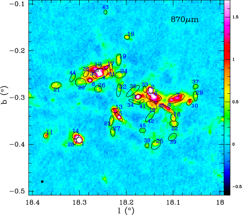
Figure 1: 870 $\mu$m dust continuum emission overlaid by the extracted Gaussian clumps for the H II region G18.2-0.3. The unit of 870 $\mu$m color bar is in ${\rm Jy~{}beam}^{-1}$. The beam size is indicated at the bottom-left corner.

2.2 Molecular line

The molecular line data is accessed from the Milky Way Galactic Ring Survey (GRS), which was performed by a Boston University (BU) and Five College Radio Astronomy Observatory (FCRAO) collaboration (Jackson et al., 2006). Using the SEQUOIA multi-pixel array receiver on the FCRAO 14 m telescope, ¹³CO (1-0) survey of the inner Galaxy was conducted. The GRS offers a sensitivity of ¡ 0.4 K, spectral resolution of 0.2 ${\rm km~{}s}^{-1}$, and angular resolution of 46^′′ with sampling 22^′′. The original intensities are on antenna temperature scale $T_{\rm A}^{*}$. To convert this to main beam temperatures $T_{\rm MB}$, $T_{\rm A}^{*}$ is divided by the main beam efficiency of 0.48. The GILDAS software package was used to reduce the molecular line data.

Table 1: Parameters of extracted clumps

No.	offset-x	offset-y	Distance	$I_{870\mu m}$	FWHMx	FWHMy	$R_{\rm eff}$	$T_{\rm dust}$	$N_{\rm H_{2}}$	Mass	Lum.
	′′	′′	kpc	${\rm Jy~{}beam}^{-1}$	′′	′′	pc	K	$\rm cm^{-2}$	$M_{\sun}$	$L_{\odot}$
1	361.00	-325.78	$3.22\pm 0.20$	4.06	46.47	40.71	0.34	30.4	2.54E+22	717	39185
2	-188.47	56.70	$3.52\pm 0.23$	3.08	56.13	35.96	0.38	30.0	1.99E+22	442	46717
3	-91.60	5.75	$\textbf{3.40}\pm\textbf{0.19}$	2.23	51.63	36.80	0.36	23.1	1.90E+22	405	16746
4	200.44	183.52	$4.92\pm 0.28$	2.22	95.34	62.25	0.92	24.7	1.76E+22	1411	34990
5	57.24	-148.65	$\textbf{3.40}\pm\textbf{0.19}$	1.80	83.31	30.06	0.41	14.7	8.27E+22	1243	5256
6	-211.70	5.40	$3.52\pm 0.23$	1.74	91.04	59.00	0.63	31.7	1.49E+22	1108	100109
7	-383.42	-5.90	$3.45\pm 0.20$	1.46	98.13	60.93	0.65	21.8	2.18E+22	1325	28660
8	280.40	131.60	$\textbf{4.92}\pm\textbf{0.28}$	1.43	41.16	28.44	0.41	22.2	1.23E+22	219	3705
9	-314.69	-85.81	$3.52\pm 0.23$	1.21	55.52	29.84	0.35	24.2	1.17E+22	294	7963
10	-486.34	-34.27	$3.40\pm 0.19$	1.11	52.32	34.65	0.35	21.3	1.30E+22	295	4045
11	617.90	-291.80	$3.36\pm 0.18$	1.03	39.90	34.39	0.30	23.6	1.06E+22	252	3702
12	246.07	228.85	$3.45\pm 0.20$	0.98	84.07	36.55	0.46	21.2	1.77E+22	802	9845
13	85.82	-97.22	$3.40\pm 0.19$	0.90	56.42	34.91	0.37	20.9	1.86E+22	561	7053
14	389.10	-291.83	$3.22\pm 0.20$	0.85	56.43	46.55	0.40	26.1	2.46E+22	870	31342
15	-194.52	-57.25	$3.45\pm 0.20$	0.80	88.83	49.44	0.55	26.2	1.07E+22	772	38883
16	-360.47	-154.53	$3.52\pm 0.23$	0.74	56.03	39.06	0.40	20.4	1.25E+22	467	4788
17	148.76	234.61	$3.45\pm 0.20$	0.73	35.63	18.85	0.22	25.9	1.27E+22	152	4829
18	-5.73	463.46	$3.45\pm 0.20$	0.70	40.44	32.84	0.30	26.3	6.31E+21	134	5164
19	57.23	291.80	$3.52\pm 0.23$	0.62	91.29	39.82	0.51	28.4	6.27E+21	331	16238
20	349.03	114.47	$4.92\pm 0.28$	0.60	85.59	70.99	0.93	24.1	5.58E+21	741	14289
21	537.83	97.23	$4.92\pm 0.28$	0.59	77.39	47.99	0.73	17.1	2.54E+22	687	5414
22	-366.17	-200.28	$3.52\pm 0.23$	0.58	66.77	41.72	0.45	18.4	1.75E+22	543	4130
23	114.41	-177.38	$3.40\pm 0.19$	0.56	82.53	30.62	0.41	22.2	7.50E+21	416	5116
24	45.78	177.34	$3.45\pm 0.20$	0.56	83.22	50.81	0.54	27.0	6.50E+21	431	19329
25	-228.84	-360.44	$3.40\pm 0.19$	0.54	89.77	57.12	0.59	22.6	6.47E+21	603	9579
26	217.41	68.65	$4.92\pm 0.28$	0.54	53.61	53.53	0.64	29.6	3.39E+21	208	11795
27	102.99	-263.20	$3.40\pm 0.19$	0.54	68.33	35.35	0.41	24.1	7.15E+21	235	6126
28	394.80	-337.58	$3.22\pm 0.20$	0.52	44.27	24.17	0.26	27.8	1.02E+22	296	16110
29	-532.10	11.45	$3.40\pm 0.19$	0.52	75.50	32.48	0.41	17.8	1.54E+22	412	3056
30	223.14	205.98	$4.92\pm 0.28$	0.51	25.54	20.91	0.28	23.4	2.10E+22	197	3311
31	114.43	217.43	$3.45\pm 0.20$	0.51	53.25	20.92	0.28	27.3	8.67E+21	162	7306
32	57.19	57.23	$3.45\pm 0.20$	0.48	80.62	35.17	0.45	26.1	5.30E+21	291	11778
33	-143.03	62.94	$3.52\pm 0.23$	0.47	50.19	27.60	0.32	31.4	6.90E+21	194	20932
34	-62.94	-34.34	$3.40\pm 0.19$	0.47	96.35	20.90	0.37	24.3	7.65E+21	243	6882
35	308.97	183.08	$4.92\pm 0.28$	0.44	53.17	32.45	0.50	21.2	1.14E+22	447	3848
36	-51.49	51.50	$3.45\pm 0.20$	0.43	88.75	41.03	0.50	27.6	5.45E+21	381	19025
37	-532.11	85.83	$3.40\pm 0.19$	0.42	39.80	35.38	0.31	17.7	1.45E+22	222	1603
38	-160.20	-366.19	$3.40\pm 0.19$	0.42	38.88	29.76	0.28	25.9	5.90E+21	118	3917
39	-354.74	-303.24	$3.40\pm 0.19$	0.41	73.45	45.71	0.48	21.2	8.40E+21	443	5025
40	-228.86	-34.33	$3.45\pm 0.20$	0.41	23.88	19.84	0.18	28.9	1.16E+22	85	5164
41	-120.16	-28.61	$3.45\pm 0.20$	0.39	38.45	19.49	0.23	27.2	6.98E+21	110	6328
42	-183.10	-143.05	$3.40\pm 0.19$	0.40	82.49	38.12	0.46	21.3	8.26E+21	411	7237
43	160.20	657.98	$3.40\pm 0.19$	0.38	33.81	25.32	0.24	23.1	6.82E+21	104	1807
44	411.95	154.48	$4.92\pm 0.28$	0.38	72.15	32.29	0.58	21.6	7.15E+21	260	3931
45	-125.87	-251.76	$3.40\pm 0.19$	0.38	49.04	35.85	0.35	25.9	5.89E+21	171	6064

• The offset (0, 0) is located at the position of $l=18.2\mbox{${}^{\circ}$}$, $b=0.3\mbox{${}^{\circ}$}$.

• The clumps 3, 5, and 8 are potentially three initial stages of massive star formation.

3 Analysis

3.1 Clump extraction

A typical terminology (e.g., Bergin & Tafalla, 2007) for clump has a physical size of 0.3 – 3 pc with a mass of about 50 – 500 $M_{\sun}$. Therefore, based on the derived effective radius in Table 1, the extracted objects are called as clump in this work.

The potential massive clumps are extracted with Gaussclumps procedure (Stutzki & Guesten, 1990; Kramer et al., 1998) in GILDAS software package in 870 $\mu$m map, assuming that the flux density of each clump is in Gaussian distribution. Gaussclumps can be used to fit a 2-dimensional clump locally to the maximum of the input cube. It then subtracts this clump from the cube, creating a residual map, and then continues with the maximum of this residual map. The procedure is repeated until a stop criterion is met, for instance when the maximum of the residual maps drops below the 3 sigma level. We just consider the clumps with peak intensity of 870 $\mu$m emission above 6$\sigma$. The measured parameters are also listed in Tables 1, and indicated with clump size in Fig. 1 and also with crosses in Fig. 2. The measured FWHMx and FWHMy have been convolved with beam size.

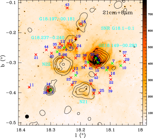
Figure 2: 21 cm dust continuum contours superimposed on image of 8 $\mu$m emission for the H II region G18.2-0.3. Several H II regions are indicated with their names. The contour levels of 21 cm emission are, respectively, 3$\sigma$, 20$\sigma$, 50$\sigma$, 100$\sigma$, 200$\sigma$, 350$\sigma$, and 520$\sigma$ with $\sigma$ = 0.002 ${\rm Jy~{}beam}^{-1}$. The unit of 8 $\mu$m color bar is in ${\rm MJy~{}sr}^{-1}$. The crosses with numbers indicate the peak positions of extracted massive clumps (see Fig. 1). Particularly, the green crosses show top 10 most massive clumps.

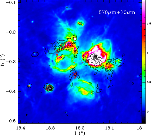
Figure 3: 870 $\mu$m dust continuum contours superimposed on image of 70 $\mu$m emission for the H II region G18.2-0.3. The contour levels of 870 $\mu$m emission start at 6$\sigma$ in steps of 8$\sigma$ with $\sigma$ = 0.054 ${\rm Jy~{}beam}^{-1}$, and its beam size is indicated at the bottom-left corner. The red crosses with numbers show three potential initial stages of massive star formation. The unit of 70 $\mu$m color bar is in MJy sr^-1.

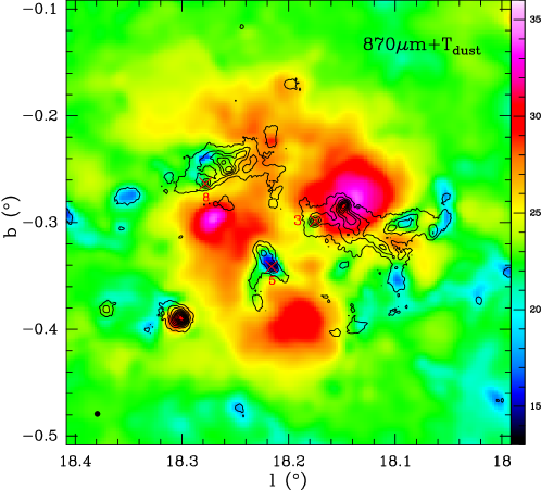
Figure 4: 870 $\mu$m dust continuum contours superimposed on image of dust temperature $T_{\rm dust}$ for the H II region G18.2-0.3. The contour levels of 870 $\mu$m emission start at 6$\sigma$ in steps of 8$\sigma$ with $\sigma$ = 0.054 ${\rm Jy~{}beam}^{-1}$, and its beam size is indicated at the bottom-left corner. The red crosses with numbers show three potential initial stages of massive star formation. The unit of $T_{\rm dust}$ color bar is in K.

3.2 Initial stage of massive star formation

Prestellar core is often suggested as the precursor of massive star formation. Prestellar cores represent a somewhat denser and more centrally-concentrated population of cores which are starless but self-gravitating (André et al., 2009). They are typically detected in sub-millimeter dust continuum emission and dense molecular gas tracers, often seen in absorption at mid- to far-infrared wavelengths (Tan et al., 2013; Chitsazzadeh et al., 2014; Wang et al., 2011, 2014; Cyganowski et al., 2014; Kong et al., 2016). However, prestellar cores are really difficult to detect, due to that they almost have nothing infrared emission.

In this work, we define infrared quiet clump as the initial stage of massive star formation. Infrared quiet clumps have all physical properties, such as cold ($T<18$ K), dense ($n>10^{5}$ cm^-3), just excluded the low luminosity ($S_{\rm 24\,\mu m}$ ¡ $(\frac{\rm 1.7\,kpc}{D})^{2}\times 15.0$ Jy; Motte et al., 2007; André et al., 2009; Russeil et al., 2010). As a potentially early stage of molecular clouds, infrared dark clouds have been discovered two decades ago as dark patches in mid-infrared (MIR) images of the Galactic plane (Perault et al., 1996; Egan et al., 1998) and many studies of the physical conditions within them have been conducted recently (Pillai et al., 2006, 2007; Wyrowski, 2008; Pillai et al., 2012; Zhang et al., 2017). H II regions do not represent the earliest stage of massive star formation, as is often claimed (e.g., Churchwell, 2002). Star formation in the Milky Way always takes place in clusters and groups within large molecular clouds (Aikawa et al., 2005; Hennebelle & Chabrier, 2008; André et al., 2009; Pagani et al., 2013). It is likely that the triggered early star formation by H II region nearby has different views from the IRDCs, such as the triggering or breeding condition. Therefore we will search for initial stage of massive star formation around an H II region complex, as is the rationale of this work.

Three clumps are proposed as potentially initial stage of massive star formation. They are, respectively, clumps No. 3, 5, and 8 listed in Table 1, and presented in Figure 3. We further searched for compact point sources in MIPS 24 $\mu$m (Carey et al., 2009; Gutermuth & Heyer, 2015), PACS 70 $\mu$m (Molinari et al., 2016), and ATLASGAL 870 $\mu$m (Csengeri et al., 2014) catalogs, and found that there exist counterparts for clumps No. 3, 5, and 8. The counterparts at 24, 70, 870 $\mu$m are listed in Table 2. Based on the definition of infrared quiet clumps ($S_{\rm 24\,\mu m}$ ¡ $(\frac{\rm 1.7\,kpc}{D})^{2}\times 15.0$ Jy), the infrared property of clumps No. 3, 5, and 8 meet this criteria.

Table 2: Point source information at 24, 70, and 870 $\mu$m

No.	$l$	$b$	MIPS${}_{\rm 24\,{\mu}m}$	$S_{\rm 24\,{\mu}m}$	PACS${}_{\rm 70\,{\mu}m}$	$S_{\rm 70\,{\mu}m}$	ATLASGAL${}_{\rm 870\,{\mu}m}$	$S_{\rm 870\,{\mu}m}$
	∘	∘		mJy		Jy		Jy
3	18.178179	-0.299098	MG018.1751-00.2985	214.881	HIGALPB018.1782-0.2991	6.569	AGAL018.174-00.299	45.38
5	18.215827	-0.341628	MG018.2157-00.3417	773.266	HIGALPB018.2158-0.3416	3.993	AGAL018.214-00.342	9.47
8	18.276361	-0.263550	MG018.2758-00.2636	463.319	HIGALPB018.2764-0.2635	7.604	AGAL018.278-00.262	22.86

3.3 Dust temperature and column density

The high-quality Herschel data cover a large wavelength range from 70 to 500 $\mu$m making it practical to obtain dust temperature maps of the H II region via fitting the SED to the multi-wavelength images on a pixel-by-pixel basis. Firstly we have followed Wang et al. (2015) to perform Fourier-Transfer (FT) based on background removal. In this method, the original images have firstly transformed into Fourier domain and separated into the low and high spatial frequency components, and then inversely Fourier transfered back into image domain. The low-frequency component corresponds to large-scale background/foreground emission, while the high-frequency component reserves the emission of interest. Detailed descriptions of the FT-based background removal method can be found in Wang et al. (2015). After removing the background/foreground emission, we have re-gridded the pixels onto the same scale of 11.5^′′, and convolved the images to a circular Gaussian beam with $\mathrm{FWHM=36.4^{\prime\prime}}$ which corresponds to the measured beam of Herschel observations at 500 $\mu$m (Traficante et al., 2011). The intensities at multi-wavelengths of each pixel have been modeled as

$$\begin{aligned} S_{\nu}=B_{\nu}(T)(1-e^{-\tau_{\nu}})\end{aligned}$$ (1)

where the Planck function $B_{\nu}(T)$ is modified by optical depth

$$\begin{aligned} \tau_{\nu}=\mu_{\mathrm{H_{2}}}m_{\mathrm{H}}\kappa_{\nu}N_{\mathrm{H_{2}}}/R_{\mathrm{gd}}.\end{aligned}$$ (2)

Here, $\mu_{\mathrm{H_{2}}}=2.8$ is the mean molecular weight adopted from Kauffmann et al. (2008), $m_{\mathrm{H}}$ is the mass of a hydrogen atom, $N_{\mathrm{H_{2}}}$ is the column density, $R_{\mathrm{gd}}=100$ is the gas to dust ratio. The dust opacity $\kappa_{\nu}$ can be expressed as a power law of frequency with

$$\begin{aligned} \kappa_{\nu}=5.0\left(\frac{\nu}{600~{}\mathrm{GHz}}\right)^{\beta}~{}\mathrm{cm^{2}g^{-1}},\end{aligned}$$ (3)

where $\kappa_{\nu}(\mathrm{600~{}GHz})=5.0~{}\mathrm{cm^{2}g^{-1}}$ adopted from Ossenkopf & Henning (1994). The dust emissivity index has been fixed to be $\beta=1.75$ according to Battersby et al. (2011). The free parameters are the dust temperature $T_{\rm dust}$ and column density $N_{\mathrm{H_{2}}}$.

The final resulted dust temperature map, which has a spatial resolution of 36.4^′′ with a pixel size of 11.5^′′, is shown in Fig. 4. Other parameters are listed in Table 1. We have to admit that the derived dust temperatures are over-estimated due to contamination from the emission of H II regions nearby.

3.4 Luminosity

The total energy radiated from an object per second (named as Boltzmann luminosity) can be expressed by

$$\begin{aligned} L_{\rm clump}=4\pi d^{2}\Omega_{\rm pix}\sum I_{\rm int},\end{aligned}$$ (4)

where $d$, $\Omega$, and $I_{\rm int}$ are the distance, solid angle, and flow of energy out of a surface at each source, respectively. The $I_{\rm int}$ for each pixel can be estimated using the resultant dust temperature and column density (see Section 3.3). The luminosities of the sources with distance measurements were calculated by integrating the frequency-integrated intensities between 10² and 10⁵ GHz within the Gaussian ellipses. The derived luminosities are listed in Table 1. We have to admit that the derived Boltzmann luminosity are also over-estimated like dust temperature due to contamination from the emission of H II regions nearby.

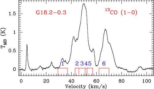
Figure 5: Averaged ¹³CO line within the whole H II region G18.2-0.3. The red windows with numbers indicate six different velocity components (see Table 4 and Fig. 6) to be further investigated.

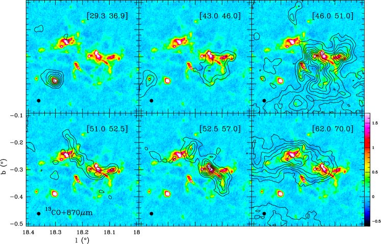
Figure 6: Integrated-velocity channel maps of ¹³CO lines superimposed on 870 $\mu$m emission for the H II region G18.2-0.3. The integrated velocity ranges are indicated in each panel with unit of ${\rm km~{}s}^{-1}$. The contour levels of the ¹³CO lines start at 3$\sigma$ in steps of 1$\sigma$ with $\sigma$ = 2.08 ${\rm K}\,{\rm km~{}s}^{-1}$. The beam size ¹³CO data is indicated at the bottom-left corner. The unit of 870 $\mu$m color bar is in ${\rm Jy~{}beam}^{-1}$.

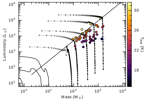
Figure 7: Luminosity-Mass diagram for sources presented in Table 1. Lines and tracks are from Saraceno et al. (1996) & Molinari et al. (2008), and depict the situation for the low-mass/low-luminosity (below the line) and high-mass/high-luminosity (above the line) regimes. The filled circles with different color indicate the sources with different dust temperatures. The three blue crosses indicate the found potential initial stages (with No. 3, 5, and 8 in Table 1) of massive star formation.

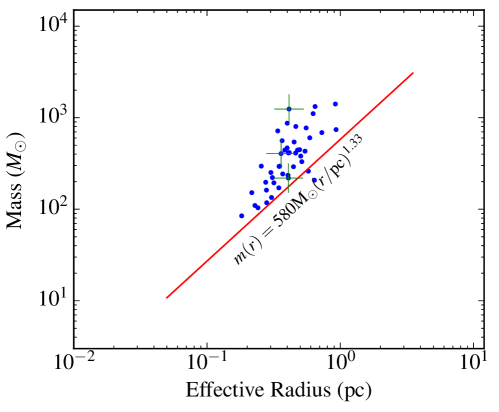
Figure 8: $Mass$-$radius$ distributions of Gaussian clumps extracted from $Gaussclumps$. The masses and effective radius are listed in Table 1. The red line delineates the threshold introduced by Kauffmann & Pillai (2010) separating the regimes under which high-mass stars can form (above) or not (below line). The clump masses in blue points (see Table 1) are derived from multiwavelength Herschel data. The three green crosses indicate the found potential initial stages (with No. 3, 5, and 8 in Table 1) of massive star formation.

3.5 Clump mass and virial mass

We just use Herschel data along with the derived dust temperatures in Section 3.3 to estimate masses of these extracted clumps. The mass is given by the integral of the column densities across the source,

$$\begin{aligned} M=\mu_{\rm H_{2}}m_{\rm H}d^{2}\int N_{\rm H_{2}}d\Omega,\end{aligned}$$ (5)

where $d$ and $\Omega$ are the distance and solid angle of the source, respectively. These corresponding and derived parameters are listed in Table 1.

The virial theorem can be used to test whether one clump is in a stable state. Under the assumption of a simple spherical clump with a density distribution of $\rho$ = constant, if ignoring magnetic fields and bulk motions of the gas (MacLaren et al., 1988; Evans, 1999),

$$\begin{aligned} M_{\rm vir}\simeq 210\,r\,\Delta V^{2}\,(M_{\sun}),\end{aligned}$$ (6)

where $r$ is adopted with the clump effective radius in pc and $\Delta V$ (listed in Figure 3) is the full width at half-maximum line width in ${\rm km~{}s}^{-1}$. The $\Delta V$ was estimated with ¹³CO line. The spatial resolution of the ¹³CO data is partly larger than the sizes of individual clumps, so we just considered the ¹³CO spectrum within one pixel corresponding with the peaked position of each clump. The virial parameter $\alpha_{\rm vir}$ is defined by $\alpha_{\rm vir}=M_{\rm vir}/M$. For the found three initial stages of massive star formation, their virial masses and virial parameters are listed in Table 3. In such dense clumps, ¹³CO line becomes optically thick, so the virial mass is likely over-estimated.

Table 3: The parameters of the found three massive clumps in initial stage

Clump	$\Delta V$	$Mass$	$M_{\rm vir}$	$\alpha_{\rm vir}$	$t_{\rm clump}$
	${\rm km~{}s}^{-1}$	$M_{\sun}$	$M_{\sun}$		Myr
3	$6.09\pm 0.06$	405	2804	6.92	1.7
5	$3.90\pm 0.08$	1243	1310	1.05	2.7
8	$6.87\pm 0.12$	219	4064	16.59	2.9

3.6 Different velocity components

In Fig. 5, we show the averaged ¹³CO line within the whole H II region G18.2-0.3. The red windows with numbers indicate six different velocity components (see Table 4 and Fig. 6) to be further investigated. The molecular clouds in different distances pile up into together, so that we often observe different velocity components in line of sight.

Dust continuum has no velocity information, so we can combine molecular line ¹³CO (1-0) to investigate the velocity correlation with the massive clumps. If the ¹³CO (1-0) emission in different integrated-velocity ranges has good correlation with any 870 $\mu$m dust continuum distribution, its corresponding velocity information can be obtained (see Figure 6).

Furthermore, the distances to the massive clumps was derived based on the Bayesian Distance Calculator (Reid et al., 2016), which leverages these results to significantly improve the accuracy and reliability of distance estimates to other sources that are known to follow spiral structure. Paron et al. (2013) listed distances of several H II regions and one SNR, which are close to the derived distances with Bayesian Distance Calculator. We think that Bayesian Distance Calculator is more reliable, so it will be adopted in this work. Based on the analysis in Figure 6, the distances of all velocity ranges for the H II region G18.2-0.3 are listed in Table 4.

In work of Paron et al. (2013), however, the authors skipped the velocity component of [62.0 70.0] ${\rm km~{}s}^{-1}$, which is actually associated with the H II region G18.237-0.240, as is unknown before. We have to note that the studied H II region complex G18.2-0.3 is indeed consisted of many different and complicated components in line of sight, and the H II region G18.237-0.240 (associated with the velocity component of [62.0 70.0] ${\rm km~{}s}^{-1}$) is located at a different arm from the other parts of the complex (see Table 4).

Table 4: Different velocity components and distances associated with G18.2-0.3

Veolcity window	1	2	3	4	5	6
Velocity (${\rm km~{}s}^{-1}$)	[29.3 36.9]	[43.0 46.0]	[46.0 51.0]	[51.0 52.5]	[52.5 57.0]	[62.0 70.0]
Line center (${\rm km~{}s}^{-1}$)	33.10	44.50	48.50	51.75	54.75	66.00
Distance (kpc)	3.22(0.20)	3.36(0.18)	3.40(0.19)	3.45(0.20)	3.52(0.23)	4.92(0.28)
Probability	0.95	1.00	1.00	0.91	0.78	0.64
Spiral arm	ScN	ScN	ScN	ScN	ScN	Nor

4 Discussion

4.1 Evolutionary time in H II regions and clump formation

We searched for the NVSS catalog and obtained a total flux of $S_{\nu}$ = 4417.0, 710.9, 796.4 mJy at $\nu$ = 1.4 GHz for the H II regions G018.148-00.283, N22, and N21, respectively (Condon et al., 1998). The flux of stellar Lyman photons $N_{\rm LyC}$, absorbed by the gas in the H II region, can be derived from the relation (Mezger et al., 1974) as

$$\left(\frac{N_{\rm LyC}}{\rm s^{-1}}\right)=\frac{4.761\times 10^{48}}{a(\nu,T_{\rm e})}\left(\frac{\nu}{\rm GHz}\right)^{0.1}\left(\frac{T_{\rm e}}{\rm K}\right)^{-0.45}\left(\frac{S_{\nu}}{\rm Jy}\right)\left(\frac{D}{\rm kpc}\right)^{2},$$ (7)

where $a(\nu,T_{\rm e})\sim 1$ is a slowly varying function tabulated by Mezger & Henderson (1967), the electron temperature of the H II region is assumed to be $T_{e}\sim$ 8000 K, and $D$ is distance. The power exponent of $T_{e}$ is small, so the result does not depend strongly on the chosen $T_{e}$. Based on above, The derived Lyman-continuum ionizing photon flux and the equivalent star style (Panagia, 1973) are listed in Table 5.

To check whether the evolutionary status of the H II regions is old enough to trigger new generation star formation nearby, we can compare the evolutionary time scales between H II regions and clump formation. We estimate their evolutionary status, using the model described by Dyson & Williams (1980) as

$$t{{}_{\rm H\,II}}=\frac{4~{}R_{s}}{7~{}c_{s}}\left[\left(\frac{R}{R_{s}}\right)^{7/4}-1\right],$$ (8)

where $R$ is the radius of H II regions obtained from the NVSS catalog (see Table 5), $c_{s}$ = 10 ${\rm km~{}s}^{-1}$ is the sound velocity in the ionized gas and $R_{s}$ is the radius of the Strömgren sphere given by $R_{s}=(3N_{\rm Lyc}/4\pi n_{0}^{2}\alpha_{B})^{1/3}$, where $N_{\rm Lyc}$ is the number of ionizing photons emitted by the star per second, $n_{0}$ = $\sim(1.0\pm 0.5)\times 10^{3}$ cm^-3 is the original ambient density, and $\alpha_{B}$ = 2.6 $\times 10^{-13}$ cm³ s^-1 is the hydrogen recombination coefficient to all levels above the ground level. Finally, we derive the dynamical age of each H II region, which is also listed in Table 5.

We estimate the fragmentation time of the three early high-mass candidates (clumps 3, 5, 8) potentially triggered by an H II region nearby according to the theoretical model from Whitworth et al. (1994):

$$t_{\rm clump}=1.56\left(\frac{\alpha_{s}}{0.2}\right)^{7/11}\left(\frac{N_{\rm Lyc}}{10^{49}}\right)^{-1/11}\left(\frac{n_{0}}{10^{3}}\right)^{-5/11}~{}\left[\rm Myr\right].$$ (9)

The turbulent velocity $\alpha_{s}$ can be estimated with line width in Table 3. Finally the derived fragmentation times for the three clumps are listed in Table 3.

Based on derived results in Tables 3 and 5, we find that the evolutionary time of the H II region is longer than the fragmentation time of the three clumps 3, 5, 8. The fragmentation time is inferred by considering the uncertainty in the total Lyman continuum photon flux and turbulent velocity. Hence, the evolutionary status of the H II regions seem to be responsible for the star formation activities around the H II regions.

4.2 The associations of initial stage of massive star formation with the H II region nearby

Are the massive clump formations triggered by the H II region nearby in Figure 2? It has been proposed that the formation of H II regions can trigger a new generation of star formation (e.g., Pomarès et al., 2009; Watson et al., 2010). In triggered star formation, one of several events might occur to compress a molecular cloud and initiate its gravitational collapse. Molecular clouds may collide with each other, or a nearby supernova explosion can be a trigger, sending shocked matter into the cloud at very high speeds (Prialnik, 2000). The triggered star formation may also happen at the waist of bipolar H II region (Deharveng et al., 2015), where the high density ionized material flows away from the central region and high density molecular material accumulates to form a torus of compressed material. Ojha et al. (2011) presented an embedded cluster along with three prominent clumps appearing to be sandwiched between the two evolved H II regions S255 and S257, and suggested that the positions of the young sources inside the gas ridge at the interface of the two H II regions favor a site of induced star formation.

Carefully checking the positions (see Section 3.6) of the three initial stages of massive star formation, we found that the clumps No. 3 and 8 are located at the border of the western H II region. Maybe the clumps No. 3 and 8 were triggered to be formed by strong stellar winds from the H II region nearby. The clump No. 5 is located at the intersection between two H II regions of bubbles N21 and N22. The case of clump No. 5 is very similar to the sandwiched star formation. It is probably that the clump No. 5 was born from the compression of the H II regions of bubbles N21 and N22. Therefore, the H II region nearby may be triggering a new generation of star formations, which will be studied in detail in our follow-up works.

Table 5: The parameters of the H II regions

H II	$R$	$D$	$S_{\rm 1.4GHz}$	log($N_{\rm LyC}$)	Stage	$t_{\rm H\,II}$
	pc	kpc	mJy			Myr
G018.148-00.283	0.68	$3.52\pm 0.23$	4417.0	48.68	O7	2.7
bubble N22	0.78	$4.92\pm 0.28$	710.9	48.17	O8.5	4.7
bubble N21	0.75	$3.40\pm 0.19$	796.4	47.89	O9.5	5.2

4.3 The property of associated massive star formation

In Fig. 8, we present the mass-size plane for the extracted clumps at 870 $\mu$m. Comparison with the high-mass star formation threshold of $m(r)>580{M_{\sun}}(r/{\rm pc})^{1.33}$ empirically proposed by Kauffmann & Pillai (2010) allows us to determine whether these clumps are capable of giving birth to massive stars. The data points are distributed above the threshold (given by the red line in Fig. 8) that discriminates between high and low mass star formation whose entries fall above and bellow the line, respectively, indicative of high-mass star-forming candidates. It appears that the most of clumps are high-mass star-forming candidates at 870 $\mu$m. Particularly, the potential three initial stages of massive star formation (marked with green crosses) are apparently located above the threshold, suggesting they are high-mass star candidates.

The derived virial masses $M_{\rm vir}$ and virial parameters $\alpha_{\rm vir}$ are listed in Table 3 for the potential three initial stages of massive star formation. Of the three clumps, $\alpha_{\rm vir}>1$ for clumps No. 3 and 8, suggesting that the clumps are not gravitationally bound, in a stable or expanding state, while $\alpha_{\rm vir}<1$ for clump No. 5, suggesting that the clump is gravitationally bound, potentially unstable, and collapsing (Hindson et al., 2013). The interaction within each clump is deserved to further study, and to understand their initial stages in detail using higher spatial resolution instrument.

4.4 How to search for initial stage of massive star formation around an H II region?

Since H II regions may trigger a new generation of star formation (Churchwell et al., 2007; Churchwell, 2008; Watson et al., 2008; Zhang & Wang, 2012), it is likely that one can obtain early star formation around H II regions. Evidences have shown that the star formation in some different evolutionary stages can be found around H II region, such as starless cores, hot cores, outflows, and protostars (Pomarès et al., 2009; Zavagno et al., 2010; Zhang & Wang, 2012). Generally the H II region has strong continuum emission at centimeter wavelength. We can use, e.g. 21 cm continuum, to trace an H II region. High-mass star formation in early stage has a cold, dense, and dark condition. It is well-known that e.g. 870 $\mu$m continuum are proposed as one good tracer. Some H II regions, such as hyper-compact H II region and hot core, may be deeply embedded in cold and dense envelope (Zhang et al., 2014), however, they show very low luminosity. These objects do not belong to the initial stage of massive star formation. Therefore, some of these compact clumps at 870 $\mu$m are not the true earliest stage. We need to further remove these clumps with weak centimeter and infrared emissions, and to get relatively early stage of star formation.

In Figure 2, the crosses with numbers are the extracted clumps associated with 870 $\mu$m and H II regions. Checking their masses and luminosities in Figure 7, we found that they almost have relatively high masses and low luminosities. In addition, in Figure 8, the mass-size relation shows that most of them are distributed above the high-mass threshold. Particularly in Figure 3 and Table 2, three dense clumps No. 3, 5, and 8 at 870 $\mu$m have weak 24 and 70 $\mu$m emission. In other word, these tree dense clumps have very weak infrared emission, but with strong emission at 870 $\mu$m, so they can be suggested as infrared quiet clumps. Their dust temperatures for No. 3, 5, 8 are 23.1, 14.7, 22.2 K (Figure 4), with masses of 405, 1243, 219 $M_{\sun}$, respectively. In Figures 7 and 8, we have highlighted the three clumps with crosses and numbers. Their properties above suggests that they are potentially initial stages of massive star formation.

5 Summary

In previous works, the early star formations were often located within IRDCs. In this work, considering star formation is in clustered condition, H II region may be triggering a new generation of star formation. It is likely that we can search for initial stage of massive star formation around H II regions. Therefore, this work is to present a method of how to search for initial stage of massive star formation around an H II region.

Towards the H II region G18.2-0.3, we carry out a multiwavelength observations to investigate its dust temperature, luminosity, mass, density, the related velocity components, and evolutionary time. By contrast and analysis, finally we find three (in 45 clump candidates associated with the H II region G18.2-0.3) potential initial stages of massive star formation, suggesting that it is feasible to search for initial stage of massive star formation around H II regions.

References

- Aikawa et al. (2005) Aikawa, Y., Herbst, E., Roberts, H., & Caselli, P. 2005, ApJ, 620, 330
- André et al. (2009) André, P., Basu, S., & Inutsuka, S. 2009, The formation and evolution of prestellar cores, ed. G. Chabrier, Structure Formation in Astrophysics, ed. G. Chabrier (Cambridge University Press), 254
- Battersby et al. (2014) Battersby, C., Ginsburg, A., Bally, J., et al. 2014, ApJ, 787, 113
- Battersby et al. (2011) Battersby, C., Bally, J., Ginsburg, A., et al. 2011, A&A, 535, A128
- Benjamin et al. (2003) Benjamin, R. A., Churchwell, E., Babler, B. L., et al. 2003, PASP, 115, 953
- Bergin & Tafalla (2007) Bergin, E. A., & Tafalla, M. 2007, ARA&A, 45, 339
- Carey et al. (2009) Carey, S. J., Noriega-Crespo, A., Mizuno, D. R., et al. 2009, PASP, 121, 76
- Chitsazzadeh et al. (2014) Chitsazzadeh, S., Di Francesco, J., Schnee, S., et al. 2014, ApJ, 790, 129
- Churchwell (2002) Churchwell, E. 2002, ARA&A, 40, 27
- Churchwell (2008) Churchwell, E. 2008, in Astronomical Society of the Pacific Conference Series, Vol. 390, Pathways Through an Eclectic Universe, ed. J. H. Knapen, T. J. Mahoney, & A. Vazdekis, 63
- Churchwell et al. (2006) Churchwell, E., Povich, M. S., Allen, D., et al. 2006, ApJ, 649, 759
- Churchwell et al. (2007) Churchwell, E., Watson, D. F., Povich, M. S., et al. 2007, ApJ, 670, 428
- Churchwell et al. (2009) Churchwell, E., Babler, B. L., Meade, M. R., et al. 2009, PASP, 121, 213
- Condon et al. (1998) Condon, J. J., Cotton, W. D., Greisen, E. W., et al. 1998, AJ, 115, 1693
- Csengeri et al. (2014) Csengeri, T., Urquhart, J. S., Schuller, F., et al. 2014, A&A, 565, A75
- Cyganowski et al. (2014) Cyganowski, C. J., Brogan, C. L., Hunter, T. R., et al. 2014, ApJ, 796, L2
- Deharveng et al. (2015) Deharveng, L., Zavagno, A., Samal, M. R., et al. 2015, A&A, 582, A1
- Dyson & Williams (1980) Dyson, J. E., & Williams, D. A. 1980, Physics of the interstellar medium
- Egan et al. (1998) Egan, M. P., Shipman, R. F., Price, S. D., et al. 1998, ApJ, 494, L199
- Evans (1999) Evans, II, N. J. 1999, ARA&A, 37, 311
- Fuller et al. (2005) Fuller, G. A., Williams, S. J., & Sridharan, T. K. 2005, A&A, 442, 949
- Green (2009) Green, D. A. 2009, Bulletin of the Astronomical Society of India, 37, 45
- Griffin et al. (2010) Griffin, M. J., Abergel, A., Abreu, A., et al. 2010, A&A, 518, L3
- Gutermuth & Heyer (2015) Gutermuth, R. A., & Heyer, M. 2015, AJ, 149, 64
- Hennebelle & Chabrier (2008) Hennebelle, P., & Chabrier, G. 2008, ApJ, 684, 395
- Hindson et al. (2013) Hindson, L., Thompson, M. A., Urquhart, J. S., et al. 2013, MNRAS, 435, 2003
- Hofner et al. (2002) Hofner, P., Delgado, H., Whitney, B., Churchwell, E., & Linz, H. 2002, ApJ, 579, L95
- Jackson et al. (2006) Jackson, J. M., Rathborne, J. M., Shah, R. Y., et al. 2006, ApJS, 163, 145
- Jiménez-Serra et al. (2014) Jiménez-Serra, I., Caselli, P., Fontani, F., et al. 2014, MNRAS, 439, 1996
- Kauffmann et al. (2008) Kauffmann, J., Bertoldi, F., Bourke, T. L., Evans, II, N. J., & Lee, C. W. 2008, A&A, 487, 993
- Kauffmann & Pillai (2010) Kauffmann, J., & Pillai, T. 2010, ApJ, 723, L7
- Kolpak et al. (2003) Kolpak, M. A., Jackson, J. M., Bania, T. M., Clemens, D. P., & Dickey, J. M. 2003, ApJ, 582, 756
- Kong et al. (2016) Kong, S., Tan, J. C., Caselli, P., et al. 2016, ApJ, 821, 94
- Kramer et al. (1998) Kramer, C., Stutzki, J., Rohrig, R., & Corneliussen, U. 1998, A&A, 329, 249
- Lockman (1989) Lockman, F. J. 1989, ApJS, 71, 469
- MacLaren et al. (1988) MacLaren, I., Richardson, K. M., & Wolfendale, A. W. 1988, ApJ, 333, 821
- Mezger & Henderson (1967) Mezger, P. G., & Henderson, A. P. 1967, ApJ, 147, 471
- Mezger et al. (1974) Mezger, P. G., Smith, L. F., & Churchwell, E. 1974, A&A, 32, 269
- Molinari et al. (2008) Molinari, S., Pezzuto, S., Cesaroni, R., et al. 2008, A&A, 481, 345
- Molinari et al. (2016) Molinari, S., Schisano, E., Elia, D., et al. 2016, A&A, 591, A149
- Motte et al. (2007) Motte, F., Bontemps, S., Schilke, P., et al. 2007, A&A, 476, 1243
- Ojha et al. (2011) Ojha, D. K., Samal, M. R., Pandey, A. K., et al. 2011, ApJ, 738, 156
- Ossenkopf & Henning (1994) Ossenkopf, V., & Henning, T. 1994, A&A, 291, 943
- Pagani et al. (2013) Pagani, L., Lesaffre, P., Jorfi, M., et al. 2013, A&A, 551, A38
- Panagia (1973) Panagia, N. 1973, AJ, 78, 929
- Paron et al. (2013) Paron, S., Weidmann, W., Ortega, M. E., Albacete Colombo, J. F., & Pichel, A. 2013, MNRAS, 433, 1619
- Perault et al. (1996) Perault, M., Omont, A., Simon, G., et al. 1996, A&A, 315, L165
- Pillai et al. (2012) Pillai, T., Caselli, P., Kauffmann, J., et al. 2012, ApJ, 751, 135
- Pillai et al. (2011) Pillai, T., Kauffmann, J., Wyrowski, F., et al. 2011, A&A, 530, A118
- Pillai et al. (2006) Pillai, T., Wyrowski, F., Carey, S. J., & Menten, K. M. 2006, A&A, 450, 569
- Pillai et al. (2007) Pillai, T., Wyrowski, F., Hatchell, J., Gibb, A. G., & Thompson, M. A. 2007, A&A, 467, 207
- Poglitsch et al. (2010) Poglitsch, A., Waelkens, C., Geis, N., et al. 2010, A&A, 518, L2
- Pomarès et al. (2009) Pomarès, M., Zavagno, A., Deharveng, L., et al. 2009, A&A, 494, 987
- Prialnik (2000) Prialnik, D. 2000, An Introduction to the Theory of Stellar Structure and Evolution
- Rathborne et al. (2010) Rathborne, J. M., Jackson, J. M., Chambers, E. T., et al. 2010, ApJ, 715, 310
- Rathborne et al. (2007) Rathborne, J. M., Simon, R., & Jackson, J. M. 2007, ApJ, 662, 1082
- Reid et al. (2016) Reid, M. J., Dame, T. M., Menten, K. M., & Brunthaler, A. 2016, ApJ, 823, 77
- Russeil et al. (2010) Russeil, D., Zavagno, A., Motte, F., et al. 2010, A&A, 515, A55
- Sanhueza et al. (2012) Sanhueza, P., Jackson, J. M., Foster, J. B., et al. 2012, ApJ, 756, 60
- Saraceno et al. (1996) Saraceno, P., Andre, P., Ceccarelli, C., Griffin, M., & Molinari, S. 1996, A&A, 309, 827
- Schuller et al. (2009) Schuller, F., Menten, K. M., Contreras, Y., et al. 2009, A&A, 504, 415
- Stutzki & Guesten (1990) Stutzki, J., & Guesten, R. 1990, ApJ, 356, 513
- Tan et al. (2013) Tan, J. C., Kong, S., Butler, M. J., Caselli, P., & Fontani, F. 2013, ApJ, 779, 96
- Traficante et al. (2011) Traficante, A., Calzoletti, L., Veneziani, M., et al. 2011, MNRAS, 416, 2932
- Walsh et al. (1997) Walsh, A. J., Hyland, A. R., Robinson, G., & Burton, M. G. 1997, MNRAS, 291, 261
- Wang et al. (2015) Wang, K., Testi, L., Ginsburg, A., et al. 2015, MNRAS, 450, 4043
- Wang et al. (2011) Wang, K., Zhang, Q., Wu, Y., & Zhang, H. 2011, ApJ, 735, 64
- Wang et al. (2014) Wang, K., Zhang, Q., Testi, L., et al. 2014, MNRAS, 439, 3275
- Watson et al. (2010) Watson, C., Hanspal, U., & Mengistu, A. 2010, ApJ, 716, 1478
- Watson et al. (2008) Watson, C., Povich, M. S., Churchwell, E. B., et al. 2008, ApJ, 681, 1341
- Whitworth et al. (1994) Whitworth, A. P., Bhattal, A. S., Chapman, S. J., Disney, M. J., & Turner, J. A. 1994, MNRAS, 268, 291
- Wyrowski (2008) Wyrowski, F. 2008, in Astronomical Society of the Pacific Conference Series, Vol. 387, Massive Star Formation: Observations Confront Theory, ed. H. Beuther, H. Linz, & T. Henning, 3
- Yuan et al. (2014) Yuan, J.-H., Wu, Y., Li, J. Z., & Liu, H. 2014, ApJ, 797, 40
- Zavagno et al. (2010) Zavagno, A., Anderson, L. D., Russeil, D., et al. 2010, A&A, 518, L101
- Zhang & Wang (2012) Zhang, C. P., & Wang, J. J. 2012, A&A, 544, A11
- Zhang & Wang (2013) Zhang, C.-P., & Wang, J.-J. 2013, Res. Astron. Astrophys., 13, 47
- Zhang et al. (2013) Zhang, C.-P., Wang, J.-J., & Xu, J.-L. 2013, A&A, 550, A117
- Zhang et al. (2014) Zhang, C.-P., Wang, J.-J., Xu, J.-L., Wyrowski, F., & Menten, K. M. 2014, ApJ, 784, 107
- Zhang et al. (2017) Zhang, C.-P., Yuan, J.-H., Li, G.-X., Zhou, J.-J., & Wang, J.-J. 2017, A&A, 598, A76
- Zhang et al. (2016) Zhang, C.-P., Li, G.-X., Wyrowski, F., et al. 2016, A&A, 585, A117