Multiscale Approach and The Convergence for the time-dependent Maxwell-Schrödinger System in Heterogeneous Nanostructures

Abstract

This paper discusses the multiscale approach and the convergence of the time-dependent Maxwell-Schrödinger system with rapidly oscillating discontinuous coefficients arising from the modeling of a heterogeneous nanostructure with a periodic microstructure. The homogenization method and the multiscale asymptotic method for the nonlinear coupled equations are presented. The efficient numerical algorithms based on the above methods are proposed. Numerical simulations are then carried out to validate the method presented in this paper.

1 Introduction

It is well-known that the classical Maxwell’s equations are widely used in the macroscopic electromagnetic theory. However, when the size of physical devices reaches the wavelength of electron, quantum effects become important even dominant and can not be neglected. To analyze and model such physical devices, coupled numerical simulations of Maxwell and Schrödinger equations need to be performed [41]. For example, an array of quantum dots is irradiated by the nearly electromagnetic field. The quantum dots, influenced by the incoming electromagnetic field, form in general a superposition of the ground and excited states, which create charge oscillations and refine the initial electromagnetic field as new source of radiation. This process leads to the interaction between the quantum dots and the electromagnetic field [39]. Hence the Maxwell equations with the quantum current density can be written as

$$\begin{array}[]{@{}l@{}}{\displaystyle\nabla\times\mathbf{E}+\frac{\partial\mathbf{B}}{\partial t}=0}\\[5.69054pt] {\displaystyle\nabla\times\mathbf{H}-\frac{\partial\mathbf{D}}{\partial t}=\mathbf{J}_{s}+\mathbf{J}_{q}}\\[5.69054pt] {\displaystyle\nabla\cdot\mathbf{D}=\rho}\\[5.69054pt] {\displaystyle\nabla\cdot\mathbf{B}=0,}\end{array}$$ (1)

where $\mathbf{E}(\mathbf{x},t)$, $\mathbf{B}(\mathbf{x},t)$, $\mathbf{H}(\mathbf{x},t)$, $\mathbf{D}(\mathbf{x},t)$, $\rho(\mathbf{x},t)$, $\mathbf{J}_{s}(\mathbf{x},t)$, $\mathbf{J}_{q}(\mathbf{x},t)$ denote the electric field intensity, the magnetic flux density, the magnetic field intensity, the electric displacement, the electric charge density, the source current density and the quantum current density, respectively. They are functions of the space $\mathbf{x}$ and time $t$. The quantum current density is derived through the method of quantum mechanics. In a linear medium, we have

$${\displaystyle\mathbf{D}=\eta\mathbf{E},\quad\mathbf{B}=\mu\mathbf{H},}$$ (2)

where $\eta=(\eta_{ij})$, $\mu=(\mu_{ij})$ are the electric permittivity and magnetic permeability, which are $3\times 3$ positive-definite matrix-valued functions of the position, respectively.

In the study of the interaction of an electron with the incoming electromagnetic field, the time-dependent Schrödinger equation can be written as follows:

$$\begin{array}[]{@{}l@{}}{\displaystyle i\hbar\frac{\partial\Psi(\mathbf{x},t)}{\partial t}=\hat{H}\Psi(\mathbf{x},t),\quad\hat{H}=\hat{H}_{0}+\hat{V}(\mathbf{x},t)},\end{array}$$ (3)

where $\hat{H}_{0}$ is the effective Hamiltonian operator in a crystal structure with the effective mass approximation (EMA) and $\hat{V}(\mathbf{x},t)$ is an interaction Hamiltonian with the incoming electromagnetic field. In this paper, we take the interaction Hamiltonian to be of the form

$${\displaystyle\hat{V}(\mathbf{x},t)=-\mathbf{E}(\mathbf{x},t)\cdot\widehat{\bm{\zeta}},}$$ (4)

where $\widehat{\bm{\zeta}}=-e\mathbf{x}$ is the electric dipole moment operator, $-e$ is the charge of the electron and $\mathbf{E}(\mathbf{x},t)\cdot\widehat{\bm{\zeta}}$ denotes the scalar product of $\mathbf{E}(\mathbf{x},t)$ and $\widehat{\bm{\zeta}}$. The quantum current density that can be injected into the time-dependent Maxwell’s equations is given as

$${\displaystyle\mathbf{J}_{q}(\mathbf{x},t)=\frac{-e\hbar}{2im}\big{(}\overline{\Psi}\nabla\Psi-\Psi\nabla\overline{\Psi}\big{)}},$$ (5)

where $m$ is the effective mass and $i$ is the imaginary unit, i.e. $i^{2}=-1$. $\overline{\Psi}$ denotes the complex conjugate of $\Psi$. As usual, here we employ the atomic units, i.e. $\hbar=e=1$.

In this paper, we consider the following time-dependent Maxwell-Schrödinger system with rapidly oscillating discontinuous coefficients given by

$$\left\{\begin{array}[]{@{}l@{}}{\displaystyle i\frac{\partial\Psi^{\varepsilon}(\mathbf{x},t)}{\partial t}=-\nabla\cdot\big{(}A(\frac{\mathbf{x}}{\varepsilon})\nabla\Psi^{\varepsilon}(\mathbf{x},t)\big{)}+\big{(}V_{c}(\frac{\mathbf{x}}{\varepsilon})-\textbf{E}^{\varepsilon}\cdot\widehat{\bm{\zeta}}+V_{xc}[\rho^{\varepsilon}]\big{)}\Psi^{\varepsilon},}\\[6.54413pt] {\displaystyle\qquad\qquad\qquad\qquad(\mathbf{x},t)\in\Omega\times(0,T),}\\[6.54413pt] {\displaystyle\eta(\frac{\mathbf{x}}{\varepsilon})\frac{\partial\mathbf{E}^{\varepsilon}(\mathbf{x},t)}{\partial t}=\mathbf{curl}\/\mathbf{H}^{\varepsilon}(\mathbf{x},t)+\mathbf{f}(\mathbf{x},t)-\mathbf{J}_{q}^{\varepsilon},\,\,\nabla\cdot\mathbf{f}=0,\,\,(\mathbf{x},t)\in\Omega\times(0,T),}\\[6.54413pt] {\displaystyle\mu(\frac{\mathbf{x}}{\varepsilon})\frac{\partial\mathbf{H}^{\varepsilon}(\mathbf{x},t)}{\partial t}=-\mathbf{curl}\/\mathbf{E}^{\varepsilon}(\mathbf{x},t),\,\,(\mathbf{x},t)\in\Omega\times(0,T),}\\[6.54413pt] {\displaystyle\nabla\cdot\big{(}\eta(\frac{\mathbf{x}}{\varepsilon})\mathbf{E}^{\varepsilon}(\mathbf{x},t)\big{)}=\rho^{\varepsilon}(\frac{\mathbf{x}}{\varepsilon},t),\quad\nabla\cdot\big{(}\mu(\frac{\mathbf{x}}{\varepsilon})\mathbf{H}^{\varepsilon}(\mathbf{x},t)\big{)}=0,\,\,(\mathbf{x},t)\in\Omega\times(0,T),}\\[6.54413pt] {\displaystyle\hat{\bm{\zeta}}=-\mathbf{x},\,\,\rho^{\varepsilon}=N{|\Psi^{\varepsilon}|}^{2},\,\,\mathbf{J}_{q}^{\varepsilon}=iN\big{[}\overline{\Psi}^{\varepsilon}A(\frac{\mathbf{x}}{\varepsilon})\nabla\Psi^{\varepsilon}-\Psi^{\varepsilon}A(\frac{\mathbf{x}}{\varepsilon})\nabla\overline{\Psi}^{\varepsilon}\big{]}.}\end{array}\right.$$ (6)

Let $\partial\Omega$ be the boundary of $\Omega$ and $\mathbf{n}=(n_{1},n_{2},n_{3})$ be the outward unit normal to $\partial\Omega$. We take (6) to hold in $\Omega$ subject to the boundary conditions

$${\displaystyle\Psi^{\varepsilon}(\mathbf{x},t)=0,\quad\mathbf{E}^{\varepsilon}(\mathbf{x},t)\times\mathbf{n}=0,\quad(\mathbf{x},t)\in\partial\Omega\times(0,T).}$$ (7)

For initial conditions we take

$${\displaystyle\Psi^{\varepsilon}(\mathbf{x},0)=\Psi_{0}(\mathbf{x}),\quad\mathbf{E}^{\varepsilon}(\mathbf{x},0)=\mathbf{\eta}^{-1}(\frac{\mathbf{x}}{\varepsilon}){\bm{\varphi}}(\mathbf{x}),\quad\mathbf{H}^{\varepsilon}(\mathbf{x},0)=\mathbf{\mu}^{-1}(\frac{\mathbf{x}}{\varepsilon}){\bm{\psi}}(\mathbf{x}),}$$ (8)

and

$${\displaystyle\nabla\cdot{\bm{\varphi}}=\nabla\cdot{\bm{\rho}^{\varepsilon}}|_{t=0},\quad\nabla\cdot{\bm{\psi}}=0,}$$ (9)

where $\nabla\cdot$ and $\nabla$ are the divergence operator and the gradient operator, respectively. $\widehat{\bm{\zeta}}$, $\rho^{\varepsilon}$ and $\mathbf{J}_{q}^{\varepsilon}$ are the electric dipole moment, the electron density and the quantum current density, respectively. Here $N$ denotes the number density of electrons.

Suppose that $\Omega\subset\mathbb{R}^{3}$ is a bounded smooth domain or a bounded polyhedral convex domain with a periodic microstructure as shown in Fig. 1. $\varepsilon>0$ is a small parameter which it represents the relative size of a periodic cell for the heterogeneous nanostructures, i.e. $0<\varepsilon=l_{p}/L<1$, where $l_{p}$ and $L$ are respectively the sizes of a periodic cell and a whole domain $\Omega$. $A(\frac{\displaystyle\mathbf{x}}{\displaystyle\varepsilon})=(a_{ij}(\frac{\displaystyle\mathbf{x}}{\displaystyle\varepsilon}))_{3\times 3}$ is the inverse of the effective masses tensor of materials. $V_{c}(\frac{\displaystyle\mathbf{x}}{\displaystyle\varepsilon})$ is the constraint step potential function. $V_{xc}(\rho^{\varepsilon})=V_{xc}(\mathbf{x},\frac{\displaystyle\mathbf{x}}{\displaystyle\varepsilon})$ is the exchange-correlation potential function. The boundary condition $\Psi^{\varepsilon}(\mathbf{x},t)=0$ on $\partial\Omega$ implies that the wave function satisfies the tight-binding state condition. The perfect conductive boundary condition for $\mathbf{E}^{\varepsilon}(\mathbf{x},t)\times\mathbf{n}=0$ is imposed on $\partial\Omega$. Here and in the sequel, the Einstein summation convention is used: summation is taken over repeated indices.

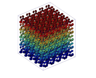
(a) (b)

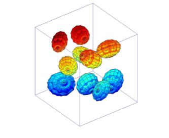
Fig. 1: (a) A semiconductor device $\Omega$ with a great of number of quantum dots; (b) the periodic cell $Q$.

We make the following assumptions:

${\bf({\rm A}_{1})}$ Let ${\bm{\xi}}=\varepsilon^{-1}\mathbf{x}$, and assume that the elements $a_{ij}({\bm{\xi}})$, $\eta_{ij}({\bm{\xi}})$ and $\mu_{ij}({\bm{\xi}})$ of matrices $A({\bm{\xi}})$, $\eta({\bm{\xi}})$ and $\mu({\bm{\xi}})$; $V_{c}({\bm{\xi}})$ and $V_{xc}(\mathbf{x},{\bm{\xi}})$ are rapidly oscillating 1-periodic real functions of space, respectively.

${\bf({\rm A}_{2})}$ The matrices $(a_{ij}({\bm{\xi}}))$, $(\eta_{ij}({\bm{\xi}}))$ and $(\mu_{ij}({\bm{\xi}}))$ are real symmetric, and satisfy the following uniform elliptic conditions in ${\bm{\xi}}$, i.e.

$$\begin{array}[]{@{}l@{}}{\displaystyle\alpha_{0}|\mathbf{y}|^{2}\leq a_{ij}({\bm{\xi}})y_{i}y_{j}\leq\alpha_{1}|\mathbf{y}|^{2},\quad\beta_{0}|\mathbf{y}|^{2}\leq\eta_{ij}({\bm{\xi}})y_{i}y_{j}\leq\beta_{1}|\mathbf{y}|^{2},}\\[5.69054pt] {\displaystyle\gamma_{0}|\mathbf{y}|^{2}\leq\mu_{ij}({\bm{\xi}})y_{i}y_{j}\leq\gamma_{1}|\mathbf{y}|^{2},\quad|\mathbf{y}|^{2}=y_{i}y_{i},}\\[5.69054pt] {\displaystyle 0<\alpha_{0}\leq\alpha_{1},\quad 0<\beta_{0}\leq\beta_{1},\quad 0<\gamma_{0}\leq\gamma_{1},\quad\forall\mathbf{y}=(y_{1},y_{2},y_{3})\in\mathbb{R}^{3},}\end{array}$$

where $\alpha_{0}$, $\alpha_{1}$, $\beta_{0}$, $\beta_{1}$, $\gamma_{0}$, $\gamma_{1}$ are constants independent of $\varepsilon$.

${\bf({\rm A}_{3})}$ $a_{ij}$, $\eta_{ij}$ , $\mu_{ij}$, $V_{c}\in L^{\infty}(\mathbb{R}^{3})$, $V_{xc}\in L^{\infty}(\Omega\times\mathbb{R}^{3})$.

${\bf({\rm A}_{4})}$ $\mathbf{f}\in L^{2}(0,T;(L^{2}(\Omega))^{3})$, $\Psi_{0}\in\mathbb{H}^{1}_{0}(\Omega)$, ${\bm{\varphi}}\in(H^{1}(\Omega))^{3}$, ${\bm{\psi}}\in(H^{1}(\Omega))^{3}$, where $H_{0}^{1}(\Omega)$ and $\mathbb{H}^{1}_{0}(\Omega)$ denote the Sobolev spaces of the real-valued and the complex-valued functions, respectively.

Maxwell-Schrödinger system with rapidly oscillating discontinuous coefficients originates from the interaction of matter and electromagnetic fields in heterogeneous nanostructures(see, e.g., [46]). There are a great number of applications in laser physics, quantum Hall effects, superconductivity and semiconductor optics and transport phenomena in heterogeneous photoelectronic devices (see, e.g., [20, 25, 43, 50]). We would like to state that, in this paper we choose the Schrödinger equation (3) with the effective mass approximation (EMA) and do not introduce the Kohn-Sham equation. There are three main reasons. First, if we use Kohn-Sham equation for the heterogeneous photoelectronic devices, it is time-consuming and difficult, due to the limitation of the computing scaling. Second, the most widely used techniques to calculate the electronic levels in nanostructures are EMA and its extension the multiband $k\cdot p$ method . They have been particularly successful in the case of heterostructures (see, e.g., [18, 50]). Thirdly, Cao et al. [8] gave a reasonable interpretation why EMA has the high accuracy for calculating the band structures of semiconductor materials in the vicinity of point $\Gamma$, from the viewpoint of mathematics. One of key points of [8] is to use an important result of [2], namely EMA in physics is equivalent to the homogenization method in mathematics under some assumptions.

The main difficult points to analyze and solve the problem (6) have the following: nonlinear, nonconvex coupled system and rapidly oscillating discontinuous coefficients. This paper focuses on discussing the multiscale approach and the convergence for the problem (6). A direct numerical method such as the finite-difference time-domain (FDTD) method or finite element (FE) method for solving the problem (6) cannot produce accurate numerical solutions unless a very fine mesh is required. On the other hand, since the elements of the coefficient matrices $A(\frac{\displaystyle\mathbf{x}}{\displaystyle\varepsilon})$ , $\eta(\frac{\displaystyle\mathbf{x}}{\displaystyle\varepsilon})$ and $\mu(\frac{\displaystyle\mathbf{x}}{\displaystyle\varepsilon})$ are discontinuous, the regularity of the solution for problem (6) maybe will be quite low (see, e.g., [16, 17]). It might be extremely difficult to derive the convergence results for FDTD or FEM.

We recall that the homogenization method gives the overall solution behavior by incorporating the fluctuations due to the heterogeneities (see, e.g., [5, 27, 40]). There are numerous important studies for the homogenization method of Maxwell’s equations, it is impossible to mention all contributions here. We refer to [5, 27, 44, 52, 53]. Other related studies have been reported in [6, 9, 10, 54, 57, 58]. For the homogenization method of Schrödinger equation, we refer to [2, 5, 8]. It should be stated that the theoretical results of the homogenization method for Schrödinger-Poisson system or Maxwell-Schrödinger system with rapidly oscillating coefficients are very limited. Recently, Zhang, Cao and Luo [56] developed the homogenization method and the multiscale method for the stationary Schrödinger-Poisson system in heterogeneous nanostructures and derived the convergence results of these methods. To the best of our knowledge, there are few theoretical results for the homogenization method and the multiscale method of Maxwell-Schrödinger system.

The main objectives of this paper are to present the homogenization method and the multiscale asymptotic methods for a kind of time-dependent Maxwell-Schrödinger system (6), to develop the associated numerical algorithms and to derive the convergence results for the present method. The new results obtained in this paper are concluded as the following:

(i) For a bounded smooth domain or a bounded polyhedral convex domain $\Omega\subset\mathbb{R}^{3}$, we present the homogenization method and the multiscale asymptotic method for the Maxwell-Schrödinger system (6) and derive the associated convergence results, see Theorems 1 and  6 and Corollary 7.

(ii) We develop the multiscale numerical algorithms based on the multiscale asymptotic expansions (55)-(57) of the solution for the problem (6) and obtain some theoretical results, see Propositions  8 and  9.

(iii) The numercial results of the multiscale asymptotic method for the Maxwell-Schrödinger system (6) without the exchange-correlation potential and with the exchange-correlation potential are provided and the validity of homogenization and multiscale method is confirmed.

The remainder of this paper is organized as follows. In section 2, we present the homogenization method and the multiscale asymptotic method for the time-dependent Maxwell-Schrödinger system (6) with rapidly oscillating discontinuous coefficients and derive the convergence results. In section 3, we use respectively the finite element method to discretize the cell problems and the modified homogenized Maxwell-Schrödinger system, and obtain the convergence results. We use the self-consistent iterative method (SCF) to solve the discrete system of the modified homogenized Maxwell-Schrödinger system. In order to accelerate the convergence speed of the iterative algorithm, the simple mixed method is applied. For more information, we refer to [24, 26, 42]. Finally, the numerical examples and some remarks are given.

2 The homogenization method and the convergence

In this section, we first introduce the results of well-posedness for the time-dependent Maxwell-Schrödinger system. Then we develop the homogenization method for the problem (6) and give the convergence result of the homogenization method.

2.1 The well-posedness of the problem (6)

Many authors have studied the existence of the solution for the time-dependent Schrödinger-Maxwell system. We recall some important studies about the problem. Nakamitsu and Tsutsumi [35] proved that the initial value problem for the Maxwell-Schrödinger system in the Lorentz gauge is globally well-posed in a space of smooth functions in dimensions one and two, and locally well-posed in dimension three. Tsutsumi[48] showed, by constructing the modified wave operator, that there exist global smooth solutions in the Coulomb gauge for a certain class of scattered data as $t\rightarrow+\infty$. The existence of global finite-energy solutions was established for the initial value problem for the Maxwell-Schrödinger system in the Coulomb, Lorentz and temporal gauges by Guo, Nakamitsu and Strauss in [23]. Ginibre and Velo [22] studied the theory of scattering for the Maxwell-Schrödinger system in space dimension 3, in the Coulomb gauge. The existence of the modified wave operators for the system in 3+1 dimension space time was derived in the special case. Nakamura and Wada [36, 37] investigated the time local and global well-posedness for the Maxwell-Schrödinger equations in Sobolev spaces in three spatial dimensions. One of the main results is that the solutions exist time globally for large data. Recently Wada [51] proved unique solvability of the Maxwell-Schrödinger equations in $\mathbb{R}^{1+2}$ spacetime. Benci and Fortunato [4] investigated the existence of charged solitons for the nonlinear Maxwell-Schrödinger equations.

In summary, we would like to state that the above results are obtained based on the following assumptions: (i) the initial problem (i.e. the Cauchy problem) of the Maxwell-Schrödinger equations with constant coefficients; (ii) no exchange-correlation potential function. Besides, they studied the well-posedness for the Maxwell-
Schrödinger equations with the vector potential and scalar potential $\mathbf{A}-\varphi$ instead of the length gauge $-e\mathbf{E}\cdot\mathbf{x}$ used in this paper (see, e.g., [15, 39]). For the well-posedness of the solution of the initial-boundary value problem for the Maxwell-Schrödinger with rapidly oscillating discontinuous coefficients seems to be open. The well-posedness of the problem (6) is not the issue of this paper. Here and in the sequel, we assume that the problem (6) has one and only one weak solution.

2.2 The homogenization method

In this section, we will study the asymptotic behaviour of the solution for the problem (6) as $\varepsilon\rightarrow 0$, i.e. the homogenization method. As usual we introduce two variables: $\mathbf{x}$ and ${\bm{\xi}=\varepsilon^{-1}\mathbf{x}}$. For simplicity, we assume that the reference cell $Q=(0,1)^{3}$ without loss of generality. For general cases, let $Q=(0,l_{1})\times(0,l_{2})\times(0,l_{3})$, we refer to a classical book [5]. For the coefficient matrices $(a_{ij}({\bm{\xi}}))$, $(\eta_{ij}({\bm{\xi}}))$ and $(\mu_{ij}({\bm{\xi}}))$, we define the following scalar cell functions:

$$\left\{\begin{array}[]{@{}l@{}}{\displaystyle{\frac{\partial}{\partial\xi_{i}}}\big{(}a_{ij}({\bm{\xi}})\displaystyle{\frac{\partial\theta_{k}^{a}({\bm{\xi}})}{\partial\xi_{j}}}\big{)}=-\frac{\partial}{\partial\xi_{i}}\big{(}a_{ik}({\bm{\xi}})\big{)},\quad{\bm{\xi}}\in Q,}\\[6.54413pt] {\displaystyle\theta_{k}^{a}({\bm{\xi}})\,\,\,\hbox{is 1-periodic}\,\,\,\hbox{in}\,\,\,{\bm{\xi}},}\\[5.97508pt] {\displaystyle\int_{Q}\theta_{k}^{a}({\bm{\xi}})\mathnormal{d}{\bm{\xi}}=0,\quad k=1,2,3,}\end{array}\right.$$ (10)

$$\left\{\begin{array}[]{@{}l@{}}{\displaystyle{\frac{\partial}{\partial\xi_{i}}}\big{(}\eta_{ij}({\bm{\xi}})\displaystyle{\frac{\partial\theta_{k}^{\eta}({\bm{\xi}})}{\partial\xi_{j}}}\big{)}=-\frac{\partial}{\partial\xi_{i}}\big{(}\eta_{ik}({\bm{\xi}})\big{)},\quad{\bm{\xi}}\in Q,}\\[6.54413pt] {\displaystyle\theta_{k}^{\eta}({\bm{\xi}})\,\,\,\hbox{is 1-periodic}\,\,\,\hbox{in}\,\,\,{\bm{\xi}},}\\[5.97508pt] {\displaystyle\int_{Q}\theta_{k}^{\eta}({\bm{\xi}})\mathnormal{d}{\bm{\xi}}=0,\quad k=1,2,3,}\end{array}\right.$$ (11)

and

$$\left\{\begin{array}[]{@{}l@{}}{\displaystyle{\frac{\partial}{\partial\xi_{i}}}\big{(}\mu_{ij}({\bm{\xi}})\displaystyle{\frac{\partial\theta_{k}^{\mu}({\bm{\xi}})}{\partial\xi_{j}}}\big{)}=-\frac{\partial}{\partial\xi_{i}}\big{(}\mu_{ik}({\bm{\xi}})\big{)},\quad{\bm{\xi}}\in Q,}\\[6.54413pt] {\displaystyle\theta_{k}^{\mu}({\bm{\xi}})\,\,\,\hbox{is 1-periodic}\,\,\,\hbox{in}\,\,\,{\bm{\xi}},}\\[5.97508pt] {\displaystyle\int_{Q}\theta_{k}^{\mu}({\bm{\xi}})\mathnormal{d}{\bm{\xi}}=0,\quad k=1,2,3.}\end{array}\right.$$ (12)

 Remark 2.1.

Under the assumptions $({\rm A}_{1})$–$({\rm A}_{3})$, the existence and uniqueness of the solutions for the cell problems (10)-(12) can be established based upon Lax-Milgram lemma.

The homogenized coefficient matrices $\widehat{A}=(\hat{a}_{ij})$, $\widehat{\eta}=(\hat{\eta}_{ij})$ and $\widehat{\mu}=(\hat{\mu}_{ij})$ are calculated by

$$\begin{array}[]{@{}l@{}}{\displaystyle\hat{a}_{ij}=\int\limits_{Q}\big{(}a_{ij}({\bm{\xi}})+a_{ik}({\bm{\xi}})\frac{\partial\theta_{j}^{a}({\bm{\xi}})}{\partial\xi_{k}}\big{)}\mathnormal{d}{\bm{\xi}},\quad\hat{\eta}_{ij}=\int\limits_{Q}\big{(}\eta_{ij}({\bm{\xi}})+\eta_{ik}({\bm{\xi}})\frac{\partial\theta_{j}^{\eta}({\bm{\xi}})}{\partial\xi_{k}}\big{)}\mathnormal{d}{\bm{\xi}},}\\[5.69054pt] {\displaystyle\qquad\qquad\qquad\hat{\mu}_{ij}=\int\limits_{Q}\big{(}\mu_{ij}({\bm{\xi}})+\mu_{ik}({\bm{\xi}})\frac{\partial\theta_{j}^{\mu}({\bm{\xi}})}{\partial\xi_{k}}\big{)}\mathnormal{d}{\bm{\xi}},\quad i,j=1,2,3.}\end{array}$$ (13)

Hence, the homogenized Maxwell-Schrödinger equations can formally be written as follows:

$$\left\{\begin{array}[]{@{}l@{}}{\displaystyle i\frac{\partial\Psi^{0}(\mathbf{x},t)}{\partial t}=-\nabla\cdot\big{(}\widehat{A}\nabla\Psi^{0}(\mathbf{x},t)\big{)}+\big{(}\langle V_{c}\rangle-\mathbf{E}^{0}\cdot\widehat{\bm{\zeta}}+V_{xc}[\rho^{0}]\big{)}\Psi^{0}(\mathbf{x},t),}\\[6.54413pt] {\displaystyle\qquad\qquad\qquad\qquad(\mathbf{x},t)\in\Omega\times(0,T),}\\[6.54413pt] {\displaystyle\widehat{\eta}\frac{\partial\mathbf{E}^{0}(\mathbf{x},t)}{\partial t}=\mathbf{curl}\/\mathbf{H}^{0}(\mathbf{x},t)+\mathbf{f}(\mathbf{x},t)-\mathbf{J}_{q}^{0},\,\,\nabla\cdot\mathbf{f}=0,\,\,(\mathbf{x},t)\in\Omega\times(0,T),}\\[6.54413pt] {\displaystyle\widehat{\mu}\frac{\partial\mathbf{H}^{0}(\mathbf{x},t)}{\partial t}=-\mathbf{curl}\/\mathbf{E}^{0}(\mathbf{x},t),\,\,(\mathbf{x},t)\in\Omega\times(0,T),}\\[6.54413pt] {\displaystyle\nabla\cdot\big{(}\widehat{\eta}\mathbf{E}^{0}(\mathbf{x},t)\big{)}=\rho^{0}(\mathbf{x},t),\quad\nabla\cdot\big{(}\widehat{\mu}\mathbf{H}^{0}(\mathbf{x},t)\big{)}=0,\,\,(\mathbf{x},t)\in\Omega\times(0,T),}\\[6.54413pt] {\displaystyle\widehat{\bm{\zeta}}=-\mathbf{x},\,\,\rho^{0}=N{|\Psi^{0}|}^{2},\,\,\mathbf{J}_{q}^{0}=iN\big{[}(\overline{\Psi}^{0})\widehat{A}\nabla\Psi^{0}-\Psi^{0}\widehat{A}\nabla\overline{\Psi}^{0}\big{]}.}\end{array}\right.$$ (14)

We take (14) to hold in $\Omega$ subject to the boundary conditions

$${\displaystyle\Psi^{0}(\mathbf{x},t)=0,\quad\mathbf{E}^{0}(\mathbf{x},t)\times\mathbf{n}=0,\quad(\mathbf{x},t)\in\partial\Omega\times(0,T).}$$ (15)

For initial conditions are taken as

$${\displaystyle\Psi^{0}(\mathbf{x},0)=\Psi_{0}(\mathbf{x}),\quad\mathbf{E}^{0}(\mathbf{x},0)=\widehat{\eta}^{-1}{\bm{\varphi}}(\mathbf{x}),\quad\mathbf{H}^{0}(\mathbf{x},0)=\widehat{\mu}^{-1}{\bm{\psi}}(\mathbf{x}).}$$ (16)

 Remark 2.2.

We observe that the homogenized problem (14) is a Maxwell-Schrödinger system with constant coefficients, it is much simpler to carry out the theoretical analysis and numerical computations than those of the original problem (6). This is the motivation of the study in this paper.

Next we derive the convergence result of the homogenization method for the problem (6).

Theorem 1.

Let $\Omega\subset\mathbb{R}^{3}$ be a bounded smooth domain or a bounded polyhedral convex domain with a periodic microstructure. Suppose that $(\Psi^{\varepsilon},\mathbf{E}^{\varepsilon},\mathbf{H}^{\varepsilon})$ be the unique weak solution of the original problem (6) without the exchange-correlation potential, i.e. $V_{xc}(\rho^{\varepsilon})\equiv 0$, and let $(\Psi^{0},\mathbf{E}^{0},\mathbf{H}^{0})$ be the unique weak solution of the associated homogenized problem (14). Under the assumptions $(A_{1})-(A_{4})$, we have

$$\begin{array}[]{@{}l@{}}{\displaystyle\Psi^{\varepsilon}\stackrel{{\scriptstyle\mathrm{w}^{\ast}}}{{\rightharpoonup}}\Psi^{0},\quad{\rm weakly\,\,star\,\,in}\quad L^{\infty}(0,T;\/\mathbb{H}_{0}^{1}(\Omega)),\quad{\rm as}\quad\varepsilon\rightarrow 0,}\\[5.69054pt] {\displaystyle\mathbf{E}^{\varepsilon}\stackrel{{\scriptstyle\mathrm{w}^{\ast}}}{{\rightharpoonup}}\mathbf{E}^{0},\quad{\rm weakly\,\,star\,\,in}\quad L^{\infty}(0,T;\/(L^{2}(\Omega))^{3}),\quad{\rm as}\quad\varepsilon\rightarrow 0,}\\[5.69054pt] {\displaystyle\mathbf{H}^{\varepsilon}\stackrel{{\scriptstyle\mathrm{w}^{\ast}}}{{\rightharpoonup}}\mathbf{H}^{0},\quad{\rm weakly\,\,star\,\,in}\quad L^{\infty}(0,T;\/(L^{2}(\Omega))^{3}),\quad{\rm as}\quad\varepsilon\rightarrow 0.}\end{array}$$ (17)

Proof.

To begin, we prove that $\|\rho^{\varepsilon}\|_{H^{-1}(\Omega)}\leq C$, where $C$ is a constant independent of $\varepsilon$. We observe that $\rho^{\varepsilon}$ in this paper is viewed as the carrier density operator $\mathcal{N}$ from Definition 2.12 of [28]. Under the assumptions $(A_{1})-(A_{4})$, one can check that $\rho^{\varepsilon}$ satisfies all conditions of Corollary 5.5 of [28]. Applying this corollary, we prove that $\|\rho^{\varepsilon}\|_{H^{-1}(\Omega)}\leq C$, where $C$ is a constant independent of $\varepsilon$.

We recall the equation $(\ref{eq:1-6})_{4}$. Under the Coulomb gauge, we have

$${\displaystyle-\nabla\cdot\big{(}\eta(\frac{\mathbf{x}}{\varepsilon})\nabla\phi^{\varepsilon}(\mathbf{x},t)\big{)}=\rho^{\varepsilon}(\mathbf{x},t),\quad\phi^{\varepsilon}\in H_{0}^{1}(\Omega),}$$

where $\mathbf{E}^{\varepsilon}(\mathbf{x},t)=-\nabla\phi^{\varepsilon}(\mathbf{x},t)$, $\phi^{\varepsilon}(\mathbf{x},t)=\phi^{\varepsilon}(\rho^{\varepsilon})$ and $t\in(0,T)$ plays the role of a parameter. Using a-priori estimates of elliptic equations (see [21, p. 181]), we get $\|\phi^{\varepsilon}(\rho^{\varepsilon})\|_{H^{1}_{0}(\Omega)}\leq C\|\rho^{\varepsilon}\|_{H^{-1}(\Omega)}\leq C$, where $C$ is a constant independent of $\varepsilon$. Therefore, for any fixed $t\in(0,T)$, there is a subsequence, without confusion still denoted by $\phi^{\varepsilon}(\rho^{\varepsilon})$, such that

$${\displaystyle\phi^{\varepsilon}\stackrel{{\scriptstyle\mathrm{w}}}{{\rightharpoonup}}\widehat{\phi}^{0}\quad\hbox{weakly \,\,in}\quad H^{1}_{0}(\Omega)\quad\hbox{as}\quad\varepsilon\rightarrow 0.}$$ (18)

Furthermore, for any fixed $t\in(0,T)$, using the homogenization result of the elliptic equation (see, e.g., [27, p. 151-152] or [5, p. 29-30]), we get

$$\begin{array}[]{@{}l@{}}{\displaystyle\mathbf{E}^{\varepsilon}\equiv-\nabla\phi^{\varepsilon}\stackrel{{\scriptstyle\mathrm{w}}}{{\rightharpoonup}}-\nabla\widehat{\phi}^{0}\stackrel{{\scriptstyle\mathrm{def}}}{{=}}\widehat{\mathbf{E}}^{0},\quad\hbox{weakly \,\, in}\quad(L^{2}(\Omega))^{3}\quad\hbox{as}\quad\varepsilon\rightarrow 0,}\\[5.69054pt] {\displaystyle\eta(\frac{\mathbf{x}}{\varepsilon})\nabla\phi^{\varepsilon}\stackrel{{\scriptstyle\mathrm{w}}}{{\rightharpoonup}}\widehat{\eta}\nabla\widehat{\phi}^{0},\quad\hbox{weakly \,\, in}\quad(L^{2}(\Omega))^{3}\quad\hbox{as}\quad\varepsilon\rightarrow 0.}\\ \end{array}$$ (19)

Thanks to $(A_{1})$ and $(A_{3})$, $V_{c}$ is a 1-periodic function in $L^{p}(Q)$ and satisfies all conditions of Theorem 2.6 of [14, p. 33]. Then we get

$${\displaystyle V_{c}(\frac{x}{\varepsilon})\rightarrow\langle V_{c}\rangle\,\,\,\hbox{weakly \,\,in}\,\,\,L^{p}(\Omega),\,\,\,\hbox{as}\,\,\,\varepsilon\rightarrow 0,\quad 1<p<+\infty.}$$ (20)

We recall $(\ref{eq:1-6})_{1}$, and consider the following modified Schödinger equation:

$${\displaystyle i\frac{\partial\widehat{\Psi}^{\varepsilon}(\mathbf{x},t)}{\partial t}=-\nabla\cdot\big{(}A(\frac{\mathbf{x}}{\varepsilon})\nabla\widehat{\Psi}^{\varepsilon}(\mathbf{x},t)\big{)}+\big{(}\langle V_{c}\rangle-\widehat{\mathbf{E}}^{0}\cdot\widehat{\bm{\zeta}}\big{)}\widehat{\Psi}^{\varepsilon}(\mathbf{x},t).}$$ (21)

Define $(u,v)=\int_{\Omega}u\bar{v}\mathnormal{d}\mathbf{x}$, $a^{\varepsilon}(u,v)=\int_{\Omega}a_{ij}(\frac{\displaystyle\mathbf{x}}{\displaystyle\varepsilon})\frac{\displaystyle\partial u}{\displaystyle\partial x_{j}}\frac{\displaystyle\partial\bar{v}}{\displaystyle\partial x_{i}}\mathnormal{d}\mathbf{x}$, where $\bar{v}$ denotes the complex conjugate of $v$. For simplicity, we assume that $\widehat{\Psi}^{\varepsilon}(\mathbf{x},0)=\Psi_{0}(\mathbf{x})\equiv 0$ without loss of generality. The variational form of (21) is the following:

$${\displaystyle-i(\dot{\widehat{\Psi}^{\varepsilon}},v)+a^{\varepsilon}(\widehat{\Psi}^{\varepsilon},v)+\big{(}(\langle V_{c}\rangle-\widehat{\mathbf{E}}^{0}\cdot\widehat{\bm{\zeta}})\widehat{\Psi}^{\varepsilon},v\big{)}=0,}$$ (22)

where $\dot{\widehat{\Psi}^{\varepsilon}}$ denotes the derivative of $\widehat{\Psi}^{\varepsilon}$ with respect to $t$. Taking $v=\dot{\widehat{\Psi}^{\varepsilon}}$ in (22) and taking the real part, we get

$${\displaystyle\frac{1}{2}\frac{d}{dt}a^{\varepsilon}(\widehat{\Psi}^{\varepsilon})=\frac{1}{2}\mathcal{R}e\frac{d}{dt}\big{(}(\langle V_{c}\rangle-\widehat{\mathbf{E}}^{0}\cdot\widehat{\bm{\zeta}})\widehat{\Psi}^{\varepsilon},\widehat{\Psi}^{\varepsilon}\big{)}+\frac{1}{2}\mathcal{R}e\big{(}(\dot{\widehat{\mathbf{E}}}^{0}\cdot\widehat{\bm{\zeta}})\widehat{\Psi}^{\varepsilon},\widehat{\Psi}^{\varepsilon}\big{)},}$$

and consequently

$${\displaystyle a^{\varepsilon}(\widehat{\Psi}^{\varepsilon}(t))=\mathcal{R}e\big{(}(\langle V_{c}\rangle-\widehat{\mathbf{E}}^{0}(t)\cdot\widehat{\bm{\zeta}})\widehat{\Psi}^{\varepsilon}(t),\widehat{\Psi}^{\varepsilon}(t)\big{)}+\mathcal{R}e\int_{0}^{t}\big{(}(\dot{\widehat{\mathbf{E}}}^{0}\cdot\widehat{\bm{\zeta}})\widehat{\Psi}^{\varepsilon},\widehat{\Psi}^{\varepsilon}\big{)}\mathnormal{d}t,}$$

where $\mathcal{R}e(u)$ denotes the real port of $u$. Hence it follows that (one obtains a preliminary estimate by taking $v=\widehat{\Psi}^{\varepsilon}$ in (22))

$${\displaystyle\|\widehat{\Psi}^{\varepsilon}\|_{L^{\infty}(0,T;\/\mathbb{H}_{0}^{1}(\Omega))}\leq C,}$$

where $C$ is a positive independent of $\varepsilon$. Then we can extract a subsequence, still denoted by $\widehat{\Psi}^{\varepsilon}$, such that

$${\displaystyle\widehat{\Psi}^{\varepsilon}\stackrel{{\scriptstyle\mathrm{w}^{\ast}}}{{\rightharpoonup}}\widehat{\Psi}^{0},\quad{\rm weakly\,\,star\,\,in}\quad L^{\infty}(0,T;\/\mathbb{H}_{0}^{1}(\Omega)),\quad{\rm as}\quad\varepsilon\rightarrow 0.}$$ (23)

Here $\widehat{\Psi}^{0}\in L^{\infty}(0,T;\mathbb{H}_{0}^{1}(\Omega))$ is the solution of the following Schrödinger equation:

$$\left\{\begin{array}[]{@{}l@{}}{\displaystyle-i(\dot{\widehat{\Psi}^{0}},v)+a^{0}(\widehat{\Psi}^{0},v)+\big{(}(\langle V_{c}\rangle-\widehat{\mathbf{E}}^{0}\cdot\widehat{\bm{\zeta}})\widehat{\Psi}^{0},v\big{)}=0,\quad\forall v\in\mathbb{H}_{0}^{1}(\Omega),}\\[5.69054pt] {\displaystyle\widehat{\Psi}^{0}(x,0)=0,}\end{array}\right.$$

where $a^{0}(u,v)=\int_{\Omega}\hat{a}_{ij}\frac{\displaystyle\partial u}{\displaystyle\partial x_{j}}\frac{\displaystyle\partial\bar{v}}{\displaystyle\partial x_{i}}\mathnormal{d}\mathbf{x}$, and $\widehat{A}=(\hat{a}_{ij})$ is the homogenized coefficient matrix of $A(\frac{\displaystyle\mathbf{x}}{\displaystyle\varepsilon})$. Following the lines of the proof of Theorem 11.4 in [14, p. 211-214] (see also the proof of Theorem 12.6 in [14, p. 231-234]), we can prove that

$$\begin{array}[]{@{}l@{}}{\displaystyle\widehat{\Psi}^{\varepsilon}\rightarrow\widehat{\Psi}^{0},\quad{\rm strongly\,\,\,in}\quad L^{2}(0,T;\/\mathbb{L}^{2}(\Omega)),\quad{\rm as}\quad\varepsilon\rightarrow 0,}\\[5.69054pt] {\displaystyle A(\frac{\mathbf{x}}{\varepsilon})\nabla\widehat{\Psi}^{\varepsilon}\stackrel{{\scriptstyle\mathrm{w}}}{{\rightharpoonup}}\widehat{A}\nabla\widehat{\Psi}^{0},\quad{\rm weakly\,\,\,in}\quad L^{2}(0,T;\/(\mathbb{L}^{2}(\Omega))^{3}),\quad{\rm as}\quad\varepsilon\rightarrow 0,}\end{array}$$ (24)

where $\mathbb{L}^{2}(\Omega)$ denotes the Sobolev space of the complex-valued functions.

If there is not the exchange-correlation potential $V_{xc}(\rho^{\varepsilon})$ in $(\ref{eq:1-6})_{1}$, subtracting $(\ref{eq:1-6})_{1}$ from (21) gives

$$\begin{array}[]{@{}l@{}}{\displaystyle i\frac{\partial(\Psi^{\varepsilon}-\widehat{\Psi}^{\varepsilon})}{\partial t}=-\nabla\cdot\big{(}A(\frac{\mathbf{x}}{\varepsilon})\nabla(\Psi^{\varepsilon}-\widehat{\Psi}^{\varepsilon})\big{)}+\big{(}V_{c}(\frac{\mathbf{x}}{\varepsilon})-\mathbf{E}^{\varepsilon}\cdot\widehat{{\bm{\zeta}}}\big{)}(\Psi^{\varepsilon}-\widehat{\Psi}^{\varepsilon})}\\[5.69054pt] {\displaystyle\qquad\qquad\qquad\quad+\big{(}(V_{c}(\frac{\mathbf{x}}{\varepsilon})-\langle V_{c}\rangle)-(\mathbf{E}^{\varepsilon}-\widehat{\mathbf{E}}^{0})\cdot\widehat{{\bm{\zeta}}}\big{)}\widehat{\Psi}^{\varepsilon}.}\end{array}$$ (25)

Setting $u^{\varepsilon}=\Psi^{\varepsilon}-\widehat{\Psi}^{\varepsilon}$, the variational form of (25) is as follows:

$$\begin{array}[]{@{}l@{}}{\displaystyle-i(\dot{u}^{\varepsilon},u^{\varepsilon})+a^{\varepsilon}(u^{\varepsilon},u^{\varepsilon})+\big{(}(V_{c}(\frac{\mathbf{x}}{\varepsilon})-\mathbf{E}^{\varepsilon}\cdot\widehat{{\bm{\zeta}}})u^{\varepsilon},u^{\varepsilon}\big{)}}\\[5.69054pt] {\displaystyle\quad=-\big{(}[(V_{c}(\frac{\mathbf{x}}{\varepsilon})-\langle V_{c}\rangle)-(\mathbf{E}^{\varepsilon}-\widehat{\mathbf{E}}^{0})\cdot\widehat{{\bm{\zeta}}}]\widehat{\Psi}^{\varepsilon},u^{\varepsilon}\big{)}.}\end{array}$$ (26)

Thanks to $(A_{3})$, $V_{c}$ is bounded. It follows from (19) that $\|\mathbf{E}^{\varepsilon}\|_{(L^{2}(\Omega))^{3}}\leq\|\phi^{\varepsilon}\|_{H_{0}^{1}(\Omega)}\leq C$, where $C$ is a constant independent of $\varepsilon$. Then, there is a sufficiently large positive number $\alpha>0$ such that

$${\displaystyle(\alpha+V_{c}(\frac{\mathbf{x}}{\varepsilon})-\mathbf{E}^{\varepsilon}\cdot\widehat{{\bm{\zeta}}})\geq\frac{\alpha}{2}>0.}$$ (27)

Hence, we take the real part in (26) and get

$$\begin{array}[]{@{}l@{}}{\displaystyle a^{\varepsilon}(u^{\varepsilon},u^{\varepsilon})+\big{(}(\alpha+V_{c}(\frac{\mathbf{x}}{\varepsilon})-\mathbf{E}^{\varepsilon}\cdot\widehat{{\bm{\zeta}}})u^{\varepsilon},u^{\varepsilon}\big{)}-(\alpha u^{\varepsilon},u^{\varepsilon})}\\[5.69054pt] {\displaystyle\quad=-\mathcal{R}e\big{(}[(V_{c}(\frac{\mathbf{x}}{\varepsilon})-\langle V_{c}\rangle)-(\mathbf{E}^{\varepsilon}-\widehat{\mathbf{E}}^{0})\cdot\widehat{{\bm{\zeta}}}]\widehat{\Psi}^{\varepsilon},u^{\varepsilon}\big{)}.}\end{array}$$ (28)

Due to the presence of the term $-(\alpha u^{\varepsilon},u^{\varepsilon})$ on the left side of (28), maybe the left side is not a coercive bilinear form. To overcome this difficulty, we use the trick of [34, p. 89]. To this end, we assume that $w^{\varepsilon}$ is the solution of the following problem:

$$\begin{array}[]{@{}l@{}}{\displaystyle a^{\varepsilon}(w^{\varepsilon},w^{\varepsilon})+\big{(}(\alpha+V_{c}(\frac{\mathbf{x}}{\varepsilon})-\mathbf{E}^{\varepsilon}\cdot\widehat{{\bm{\zeta}}})w^{\varepsilon},w^{\varepsilon}\big{)}+(\alpha w^{\varepsilon},w^{\varepsilon})}\\[5.69054pt] {\displaystyle\quad=-\mathcal{R}e\big{(}[(V_{c}(\frac{\mathbf{x}}{\varepsilon})-\langle V_{c}\rangle)-(\mathbf{E}^{\varepsilon}-\widehat{\mathbf{E}}^{0})\cdot\widehat{{\bm{\zeta}}}]\widehat{\Psi}^{\varepsilon},w^{\varepsilon}\big{)}.}\end{array}$$ (29)

We thus obtain

$${\displaystyle\|w^{\varepsilon}\|_{L^{\infty}(0,T;\/\mathbb{H}_{0}^{1}(\Omega))}\leq C\big{\{}\|V_{c}(\frac{\mathbf{x}}{\varepsilon})-\langle V_{c}\rangle\|_{H^{-1}(\Omega)}+\|\mathbf{E}^{\varepsilon}-\widehat{\mathbf{E}}^{0}\|_{L^{2}(0,T;\/H^{-1}(\Omega))}\big{\}}.}$$

From (19) and (20), we have

$${\displaystyle\|w^{\varepsilon}\|_{L^{\infty}(0,T;\/\mathbb{H}_{0}^{1}(\Omega))}\rightarrow 0,\quad{\rm as}\quad\varepsilon\rightarrow 0.}$$ (30)

Similarly to (4.18) of [34, p. 91], we get $(I+K)u^{\varepsilon}=w^{\varepsilon}$, where $I$ is an identity operator from $\mathbb{L}^{2}(\Omega)\rightarrow\mathbb{L}^{2}(\Omega)$, and the operator $K$ is a bounded and compact map from $\mathbb{L}^{2}(\Omega)\rightarrow\mathbb{L}^{2}(\Omega)$ shown as in (4.15) of [34, p. 90]. Furthermore, we have $\|u^{\varepsilon}\|_{\mathbb{L}^{2}(\Omega)}\leq C\|w^{\varepsilon}\|_{\mathbb{L}^{2}(\Omega)}$, where $C$ is a constant independent of $\varepsilon$.

Combining (28) and (30) implies

$$\begin{array}[]{@{}l@{}}{\displaystyle\|u^{\varepsilon}\|_{L^{\infty}(0,T;\/\mathbb{H}_{0}^{1}(\Omega))}\leq C\big{\{}\|w^{\varepsilon}\|_{L^{\infty}(0,T;\/\mathbb{L}^{2}(\Omega))}+\|V_{c}(\frac{\mathbf{x}}{\varepsilon})-\langle V_{c}\rangle\|_{H^{-1}(\Omega)}}\\[5.69054pt] {\displaystyle\quad+\|\mathbf{E}^{\varepsilon}-\widehat{\mathbf{E}}^{0}\|_{L^{2}(0,T;\/H^{-1}(\Omega))}\big{\}}\rightarrow 0,\quad{\rm as}\quad\varepsilon\rightarrow 0,}\end{array}$$

and consequently

$${\displaystyle\|\Psi^{\varepsilon}-\widehat{\Psi}^{\varepsilon}\|_{L^{\infty}(0,T;\/\mathbb{H}_{0}^{1}(\Omega))}\rightarrow 0,\quad{\rm as}\quad\varepsilon\rightarrow 0.}$$ (31)

We recall $(\ref{eq:1-6})_{5}$, and combining (24) and (31) gives

$${\displaystyle\mathbf{J}_{q}^{\varepsilon}\stackrel{{\scriptstyle\mathrm{w}}}{{\rightharpoonup}}\widehat{\mathbf{J}}_{q}^{0},\quad{\rm weakly\,\,in}\quad L^{2}(0,T;\/(L^{2}(\Omega))^{3}),\quad{\rm as}\quad\varepsilon\rightarrow 0.}$$ (32)

Using Theorem 4.1 in Chapter 7 of [19] and following the lines of the proof of Theorem 4.5 in [5, p. 666](see also [44, p. 125]), we prove

$$\begin{array}[]{@{}l@{}}{\displaystyle\mathbf{E}^{\varepsilon}\stackrel{{\scriptstyle\mathrm{w}^{\ast}}}{{\rightharpoonup}}\widehat{\mathbf{E}}^{0},\quad{\rm weakly\,\,star\,\,in}\quad L^{\infty}(0,T;\/(L^{2}(\Omega))^{3}),\quad{\rm as}\quad\varepsilon\rightarrow 0,}\\[5.69054pt] {\displaystyle\mathbf{H}^{\varepsilon}\stackrel{{\scriptstyle\mathrm{w}^{\ast}}}{{\rightharpoonup}}\widehat{\mathbf{H}}^{0},\quad{\rm weakly\,\,star\,\,in}\quad L^{\infty}(0,T;\/(L^{2}(\Omega))^{3}),\quad{\rm as}\quad\varepsilon\rightarrow 0.}\end{array}$$ (33)

Let us turn to the proof of $\widehat{\phi}^{0}=\phi^{0}(\rho^{0})$. Combining (24) and (31), for any fixed $t\in(0,T)$, we have

$${\displaystyle\rho^{\varepsilon}\equiv N|\Psi^{\varepsilon}|^{2}\stackrel{{\scriptstyle\mathrm{w}}}{{\rightharpoonup}}N|\widehat{\Psi}^{0}|^{2}\equiv\widehat{\rho}^{0},\quad{\rm weakly\,\,\,in}\quad L^{2}(\Omega),\quad{\rm as}\quad\varepsilon\rightarrow 0,}$$

and consequently

$${\displaystyle\|\rho^{\varepsilon}-\widehat{\rho}^{0}\|_{H^{-1}(\Omega)}\rightarrow 0,\quad{\rm as}\quad\varepsilon\rightarrow 0.}$$ (34)

For any fixed $t\in(0,T)$, let $\widetilde{\phi}^{\varepsilon}(\mathbf{x},t)$ be the solution of the following elliptic equation:

$$\left\{\begin{array}[]{lll}{\displaystyle-\frac{\partial}{\partial x_{i}}\big{(}\eta_{ij}(\frac{x}{\varepsilon})\frac{\partial\widetilde{\phi}^{\varepsilon}(\mathbf{x},t)}{\partial x_{j}}\big{)}=\widehat{\rho}^{0}(\mathbf{x},t),\quad\mathbf{x}\in\Omega,}\\[5.69054pt] {\displaystyle\widetilde{\phi}^{\varepsilon}(\mathbf{x},t)=0,\quad\mathbf{x}\in\partial\Omega,}\end{array}\right.$$ (35)

where $t$ plays the role of a parameter. As usual we use the convergence result of the homogenization method for the linear elliptic equations (see, e.g., Theorem 3.1 of [5] or Theorem 6.1 of [14]) and obtain

$$\begin{array}[]{@{}l@{}}{\displaystyle\widetilde{\phi}^{\varepsilon}\rightarrow\widehat{\phi}^{0}(\widehat{\rho}^{0})\quad\hbox{weakly \,\,in}\,\,\,H^{1}_{0}(\Omega),\,\,\,\hbox{as}\,\,\,\varepsilon\rightarrow 0,}\\[5.69054pt] {\displaystyle\widetilde{\phi}^{\varepsilon}\rightarrow\widehat{\phi}^{0}(\widehat{\rho}^{0})\quad\hbox{strongly \,\,in}\,\,\,L^{2}(\Omega),\,\,\,\hbox{as}\,\,\,\varepsilon\rightarrow 0.}\end{array}$$ (36)

Subtracting $(\ref{eq:1-6})_{4}$ from (35) and using a priori estimates for elliptic equations, we get

$${\displaystyle\|\phi^{\varepsilon}(\rho^{\varepsilon})-\widetilde{\phi}^{\varepsilon}\|_{H^{1}_{0}(\Omega)}\leq C\|\rho^{\varepsilon}-\widehat{\rho}^{0}\|_{H^{-1}(\Omega)}\rightarrow 0,\quad\hbox{as}\,\,\,\varepsilon\rightarrow 0.}$$ (37)

For any fixed $t\in(0,T)$, combining (18), (34) and (36) gives $\widehat{\phi}^{0}(\mathbf{x},t)=\widehat{\phi}^{0}(\widehat{\rho}^{0}(\mathbf{x},t))$. On the other hand, we assume that the problem (6) without the exchange-correlation potential and the associated homogenized problem (14) have the unique weak solutions, respectively. Consequently, the convergence (24) takes place for the whole sequences. Therefore, we get $\phi^{0}=\phi^{0}(n^{0})$. From this, we have $\widehat{\Psi}^{0}=\Psi^{0}$, $\widehat{\mathbf{E}}^{0}=\mathbf{E}^{0}$ and $\widehat{\mathbf{H}}^{0}=\mathbf{H}^{0}$. Therefore, we complete the proof of Theorem 1.  ∎

Corollary 2.

If there is the exchange-correlation potential in (6), which it is Lipschitz continuous and the corresponding Lipschitz constant is sufficiently small, and other conditions are the same as Theorem 1, then we can derive the similar convergence results to those of Theorem 1.

In fact, here we consider the following modified Schödinger equation:

$${\displaystyle i\frac{\partial\widehat{\Psi}^{\varepsilon}(\mathbf{x},t)}{\partial t}=-\nabla\cdot\big{(}A(\frac{\mathbf{x}}{\varepsilon})\nabla\widehat{\Psi}^{\varepsilon}(\mathbf{x},t)\big{)}+\big{(}\langle V_{c}\rangle-\widehat{\mathbf{E}}^{0}\cdot\widehat{\bm{\zeta}}+V_{xc}(\widehat{\rho}^{\varepsilon})\big{)}\widehat{\Psi}^{\varepsilon}(\mathbf{x},t),}$$ (38)

where $\widehat{\rho}^{\varepsilon}=N|\widehat{\Psi}^{\varepsilon}|^{2}$. If the exchange-correlation potential in (6) is Lipschitz continuous and the corresponding Lipschitz constant is sufficiently small, then we can prove that the self-consistent iterative method (SCF) is convergent. Following the lines of the proofs of (22)-(37), we can complete the proof of Corollary 2.

 Remark 2.3.

If there is the generic exchange-correlation potential (see, e.g., [33, p. 152-169]), then the convergence result of the homogenization method for the problem (6) is not known to authors yet.

3 The multiscale asymptotic method and the main convergence theorems

Numerous numerical results have shown that, if $\varepsilon>0$ is not sufficiently small, the accuracy of the homogenization method may not be satisfactory (see, e.g., [7, 9, 10, 56, 57]). Hence one hopes to seek the multiscale asymptotic methods and the associated numerical algorithms in the real applications. In this section, we first formally present the multiscale asymptotic expansions of the solution of (6), and then we derive the convergence result of the multiscale method.

3.1 The multiscale asymptotic expansions

Let ${\bm{\xi}}=\varepsilon^{-1}\mathbf{x}$, for the coefficient matrices $A({\bm{\xi}})=(a_{ij}({\bm{\xi}}))$, $\eta({\bm{\xi}})=(\eta_{ij}({\bm{\xi}}))$ and $\mu({\bm{\xi}})=(\mu_{ij}({\bm{\xi}}))$, we will define three sets of cells functions: $\theta_{k}^{a}({\bm{\xi}})$, $\theta_{kl}^{a}({\bm{\xi}})$; $\theta_{k}^{\eta}({\bm{\xi}})$, $\theta_{kl}^{\eta}({\bm{\xi}})$, $\Theta_{1}^{\eta}({\bm{\xi}})$, $\Theta_{2}^{\eta}({\bm{\xi}})$; $\theta_{k}^{\mu}({\bm{\xi}})$, $\theta_{kl}^{\mu}({\bm{\xi}})$, $\Theta_{1}^{\mu}({\bm{\xi}})$, $\Theta_{2}^{\mu}({\bm{\xi}})$, $k,l=1,2,3$, where $\theta_{k}^{a}({\bm{\xi}})$, $\theta_{kl}^{a}({\bm{\xi}})$, $\theta_{k}^{\eta}({\bm{\xi}})$, $\theta_{kl}^{\eta}({\bm{\xi}})$, $\theta_{k}^{\mu}({\bm{\xi}})$, $\theta_{kl}^{\mu}({\bm{\xi}})$ are scalar cell functions and $\Theta_{1}^{\eta}({\bm{\xi}})$, $\Theta_{2}^{\eta}({\bm{\xi}})$ , $\Theta_{1}^{\mu}({\bm{\xi}})$, $\Theta_{2}^{\mu}({\bm{\xi}})$ are matrix-valued cell functions defined in the unit cell $Q$. The scalar cells functions $\theta_{k}^{a}({\bm{\xi}})$, $\theta_{kl}^{a}({\bm{\xi}})$, $\theta_{k}^{\eta}({\bm{\xi}})$, $\theta_{kl}^{\eta}({\bm{\xi}})$, $\theta_{k}^{\mu}({\bm{\xi}})$, $\theta_{kl}^{\mu}({\bm{\xi}})$ are defined in turn

$$\left\{\begin{array}[]{@{}l@{}}{\displaystyle\frac{\partial}{\partial\xi_{i}}\big{(}a_{ij}({\bm{\xi}})\frac{\partial\theta_{k}^{a}({\bm{\xi}})}{\partial\xi_{j}}\big{)}=-\frac{\partial a_{ik}({\bm{\xi}})}{\partial\xi_{i}},\quad{\bm{\xi}}\in Q,}\\[5.69054pt] {\displaystyle\theta_{k}^{a}({\bm{\xi}})=0,\quad{\bm{\xi}}\in\partial Q,}\end{array}\right.$$ (39)

$$\left\{\begin{array}[]{@{}l@{}}{\displaystyle\frac{\partial}{\partial\xi_{i}}\big{(}a_{ij}({\bm{\xi}})\frac{\partial\theta_{kl}^{a}({\bm{\xi}})}{\partial\xi_{j}}\big{)}=-\frac{\partial\big{(}a_{ik}({\bm{\xi}})\theta_{l}^{a}({\bm{\xi}})\big{)}}{\partial\xi_{i}}}\\[8.53581pt] {\displaystyle\qquad-a_{kj}({\bm{\xi}})\frac{\partial\theta_{l}^{a}({\bm{\xi}})}{\partial\xi_{j}}-a_{kl}({\bm{\xi}})+\hat{a}_{kl},\quad{\bm{\xi}}\in Q,}\\ {\displaystyle\theta_{kl}^{a}({\bm{\xi}})=0,\quad{\bm{\xi}}\in\partial Q},\end{array}\right.$$ (40)

$$\left\{\begin{array}[]{@{}l@{}}{\displaystyle\frac{\partial}{\partial\xi_{i}}\big{(}\eta_{ij}({\bm{\xi}})\frac{\partial\theta_{k}^{\eta}({\bm{\xi}})}{\partial\xi_{j}}\big{)}=-\frac{\partial\eta_{ik}({\bm{\xi}})}{\partial\xi_{i}},\quad{\bm{\xi}}\in Q,}\\[5.69054pt] \theta_{k}^{\eta}({\bm{\xi}})=0,\quad{\bm{\xi}}\in\partial Q,\end{array}\right.$$ (41)

$$\left\{\begin{array}[]{@{}l@{}}{\displaystyle\frac{\partial}{\partial\xi_{i}}\big{(}\eta_{ij}({\bm{\xi}})\frac{\partial\theta_{kl}^{\eta}({\bm{\xi}})}{\partial\xi_{j}}\big{)}=-\frac{\partial\big{(}\eta_{ik}({\bm{\xi}})\theta_{l}^{\eta}({\bm{\xi}})\big{)}}{\partial\xi_{i}}}\\[8.53581pt] {\displaystyle\qquad-\eta_{kj}({\bm{\xi}})\frac{\partial\theta_{l}^{\eta}({\bm{\xi}})}{\partial\xi_{j}}-\eta_{kl}({\bm{\xi}})+\hat{\eta}_{kl},\quad{\bm{\xi}}\in Q,}\\ {\displaystyle\theta_{kl}^{\eta}({\bm{\xi}})=0,\quad{\bm{\xi}}\in\partial Q},\end{array}\right.$$ (42)

$$\left\{\begin{array}[]{@{}l@{}}{\displaystyle\frac{\partial}{\partial\xi_{i}}\big{(}\mu_{ij}({\bm{\xi}})\frac{\partial\theta_{k}^{\mu}({\bm{\xi}})}{\partial\xi_{j}}\big{)}=-\frac{\partial\mu_{ik}({\bm{\xi}})}{\partial\xi_{i}},\quad{\bm{\xi}}\in Q,}\\[5.69054pt] {\displaystyle\theta_{k}^{\mu}({\bm{\xi}})=0,\quad{\bm{\xi}}\in\partial Q,}\end{array}\right.$$ (43)

and

$$\left\{\begin{array}[]{@{}l@{}}{\displaystyle\frac{\partial}{\partial\xi_{i}}\big{(}\mu_{ij}({\bm{\xi}})\frac{\partial\theta_{kl}^{\mu}({\bm{\xi}})}{\partial\xi_{j}}\big{)}=-\frac{\partial\big{(}\mu_{ik}({\bm{\xi}})\theta_{l}^{\mu}({\bm{\xi}})\big{)}}{\partial\xi_{i}}}\\ {\displaystyle\qquad-\mu_{kj}({\bm{\xi}})\frac{\partial\theta_{l}^{\mu}({\bm{\xi}})}{\partial\xi_{j}}-\mu_{kl}({\bm{\xi}})+\hat{\mu}_{kl},\quad{\bm{\xi}}\in Q,}\\[8.53581pt] {\displaystyle\theta_{kl}^{\mu}({\bm{\xi}})=0,\quad{\bm{\xi}}\in\partial Q},\end{array}\right.$$ (44)

where the homogenized coefficient matrices $\widehat{A}=(\hat{a}_{kl})$, $\widehat{\eta}=(\hat{\eta}_{kl})$ and $\widehat{\mu}=(\hat{\mu}_{kl})$ are similarly given in (13).

 Remark 3.1.

Under the assumptions $({\rm A}_{1})$–$({\rm A}_{3})$, the existence and uniqueness of the solutions for the cell problems (39)-(44) can be established based upon Lax-Milgram lemma. It should be mentioned the problems (39)-(44) require the homogeneous Dirichlet’s boundary conditions instead of the usual periodic boundary conditions.

Next we give the definitions of the matrix-valued cell functions $\mathbf{\Theta}_{1}^{\eta}({\bm{\xi}})$, $\mathbf{\Theta}_{2}^{\eta}({\bm{\xi}})$, $\mathbf{\Theta}_{1}^{\mu}({\bm{\xi}})$ and $\mathbf{\Theta}_{2}^{\mu}({\bm{\xi}})$. Let $\eta^{-1}({\bm{\xi}})$ and $\mu^{-1}({\bm{\xi}})$ denote the inverse matrices of $\eta({\bm{\xi}})$ and $\mu({\bm{\xi}})$, respectively. We define $\mathbf{\Theta}_{1,p}^{\eta}({\bm{\xi}})$, $\mathbf{\Theta}_{1,p}^{\mu}({\bm{\xi}})$, $p=1,2,3$ in the following ways:

$$\left\{\begin{array}[]{l@{}}{\displaystyle\mathbf{curl}_{{\bm{\xi}}}(\eta^{-1}({\bm{\xi}})\mathbf{curl}_{{\bm{\xi}}}\Theta^{\eta}_{1,p}({\bm{\xi}}))=-\mathbf{curl}_{{\bm{\xi}}}(\eta^{-1}({\bm{\xi}})\mathbf{e}_{p}),\quad{\bm{\xi}}\in Q,}\\[5.69054pt] {\displaystyle\nabla_{{\bm{\xi}}}\cdot\Theta^{\eta}_{1,p}({\bm{\xi}})=0,\quad{\bm{\xi}}\in Q,}\\[5.69054pt] {\displaystyle\Theta^{\eta}_{1,p}({\bm{\xi}})\times{\bm{\nu}}=0,\quad{\bm{\xi}}\in\partial Q,\quad p=1,2,3,}\end{array}\right.$$ (45)

$$\left\{\begin{array}[]{l@{}}{\displaystyle\mathbf{curl}_{{\bm{\xi}}}(\mu^{-1}({\bm{\xi}})\mathbf{curl}_{{\bm{\xi}}}\Theta^{\mu}_{1,p}({\bm{\xi}}))=-\mathbf{curl}_{{\bm{\xi}}}(\mu^{-1}({\bm{\xi}})\mathbf{e}_{p}),\quad{\bm{\xi}}\in Q,}\\[5.69054pt] {\displaystyle\nabla_{{\bm{\xi}}}\cdot\Theta^{\mu}_{1,p}({\bm{\xi}})=0,\quad{\bm{\xi}}\in Q,}\\[5.69054pt] {\displaystyle\Theta^{\mu}_{1,p}({\bm{\xi}})\times{\bm{\nu}}=0,\quad{\bm{\xi}}\in\partial Q,\quad p=1,2,3,}\end{array}\right.$$ (46)

where $\Theta_{1,p}^{\eta}({\bm{\xi}})$ and $\Theta_{1,p}^{\mu}({\bm{\xi}})$, $p=1,2,3$ are the vector-valued functions, ${\bm{\nu}}=(\nu_{1},\nu_{2},\nu_{3})$ is the outward unit normal to $\partial Q$, $\mathbf{e}_{1}=\{1,0,0\}^{T}$, $\mathbf{e}_{2}=\{0,1,0\}^{T}$, $\mathbf{e}_{3}=\{0,0,1\}^{T}$, $\mathbf{a}^{T}$ denotes the transpose of a vector $\mathbf{a}$. Let

$${\displaystyle\Theta_{1}^{\eta}(\mathbf{\xi})=(\Theta^{\eta}_{1,1}(\mathbf{\xi}),\Theta^{\eta}_{1,2}(\mathbf{\xi}),\Theta^{\eta}_{1,3}(\mathbf{\xi})),\quad\Theta_{1}^{\mu}(\mathbf{\xi})=(\Theta^{\mu}_{1,1}(\mathbf{\xi}),\Theta^{\mu}_{1,2}(\mathbf{\xi}),\Theta^{\mu}_{1,3}(\mathbf{\xi})).}$$

 Remark 3.2.

The definitions of $\Theta_{1,p}^{\eta}({\bm{\xi}})$, $\Theta_{1,p}^{\mu}({\bm{\xi}})$, $p=1,2,3$ in (45) and (46) are similar to (4.128) of [5, p. 663]. However, the essential difference is that we take a perfect conductor boundary condition instead of the periodic boundary condition of [5]. Similarly to (4.128) of [5, p. 663], under the assumptions $({\rm A}_{1})$–$({\rm A}_{3})$, the existence and uniqueness of problems (45) and (46) can be established based upon Lax-Milgram lemma.

Following the idea of [7], we define the second-order vector-valued cell functions $\Theta_{2,p}^{\eta}({\bm{\xi}})$ and $\Theta_{2,p}^{\mu}({\bm{\xi}})$ as follows:

$$\left\{\begin{array}[]{l@{}}{\displaystyle\mathbf{curl}_{{\bm{\xi}}}(\eta^{-1}({\bm{\xi}})\mathbf{curl}_{{\bm{\xi}}}\Theta^{\eta}_{2,p}({\bm{\xi}}))=-\mathbf{curl}_{{\bm{\xi}}}(\eta^{-1}({\bm{\xi}})\Theta^{\eta}_{1,p}({\bm{\xi}}))}\\[5.69054pt] {\displaystyle\quad-\eta^{-1}({\bm{\xi}})\mathbf{curl}_{{\bm{\xi}}}\Theta^{\eta}_{1,p}({\bm{\xi}})-\eta^{-1}({\bm{\xi}})\mathbf{e}_{p}+\widehat{\eta}^{-1}\mathbf{e}_{p}+\nabla_{{\bm{\xi}}}\zeta_{2,p}^{\eta}({\bm{\xi}}),\quad{\bm{\xi}}\in Q,}\\[5.69054pt] {\displaystyle\nabla_{{\bm{\xi}}}\cdot\Theta^{\eta}_{2,p}({\bm{\xi}})=0,\quad{\bm{\xi}}\in Q,}\\[5.69054pt] {\displaystyle\Theta^{\eta}_{2,p}({\bm{\xi}})\times{\bm{\nu}}=0,\quad{\bm{\xi}}\in\partial Q,\quad p=1,2,3,}\end{array}\right.$$ (47)

and

$$\left\{\begin{array}[]{l@{}}{\displaystyle\mathbf{curl}_{{\bm{\xi}}}(\mu^{-1}({\bm{\xi}})\mathbf{curl}_{{\bm{\xi}}}\Theta^{\mu}_{2,p}({\bm{\xi}}))=-\mathbf{curl}_{{\bm{\xi}}}(\mu^{-1}({\bm{\xi}})\Theta^{\mu}_{1,p}({\bm{\xi}}))}\\[5.69054pt] {\displaystyle\quad-\mu^{-1}({\bm{\xi}})\mathbf{curl}_{{\bm{\xi}}}\Theta^{\mu}_{1,p}({\bm{\xi}})-\mu^{-1}({\bm{\xi}})\mathbf{e}_{p}+\widehat{\mu}^{-1}\mathbf{e}_{p}+\nabla_{{\bm{\xi}}}\zeta_{2,p}^{\mu}({\bm{\xi}}),\quad{\bm{\xi}}\in Q,}\\[5.69054pt] {\displaystyle\nabla_{{\bm{\xi}}}\cdot\Theta^{\mu}_{2,p}({\bm{\xi}})=0,\quad{\bm{\xi}}\in Q,}\\[5.69054pt] {\displaystyle\Theta^{\mu}_{2,p}({\bm{\xi}})\times{\bm{\nu}}=0,\quad{\bm{\xi}}\in\partial Q,\quad p=1,2,3.}\end{array}\right.$$ (48)

By using (11.46) of [5, p. 145], the homogenized coefficient matrices $\widehat{\eta}^{-1}$ and $\widehat{\mu}^{-1}$ are calculated by

$$\begin{array}[]{l@{}}{\displaystyle\widehat{\eta}^{-1}=\mathcal{M}\Bigl{(}\eta^{-1}({\bm{\xi}})+\eta^{-1}({\bm{\xi}})\,\mathbf{curl}_{{\bm{\xi}}}\,\Theta_{1}^{\eta}({\bm{\xi}})\Bigr{)},}\\[5.69054pt] {\displaystyle\widehat{\mu}^{-1}=\mathcal{M}\Bigl{(}\mu^{-1}({\bm{\xi}})+\mu^{-1}({\bm{\xi}})\,\mathbf{curl}_{{\bm{\xi}}}\,\Theta_{1}^{\mu}({\bm{\xi}})\Bigr{)},}\end{array}$$ (49)

where the matrix-valued cell functions $\Theta_{1}^{\eta}({\bm{\xi}})=(\Theta^{\eta}_{1,1}({\bm{\xi}})$, $\Theta^{\eta}_{1,2}({\bm{\xi}})$, $\Theta^{\eta}_{1,3}({\bm{\xi}}))$ and $\Theta_{1}^{\mu}({\bm{\xi}})=(\Theta^{\mu}_{1,1}({\bm{\xi}}),\Theta^{\mu}_{1,2}({\bm{\xi}}),\Theta^{\mu}_{1,3}({\bm{\xi}}))$ are defined in (45) and (46), respectively, $\mathcal{M}v=\int_{Q}v({\bm{\xi}})\mathnormal{d}{\bm{\xi}}$. The functions $\zeta_{2,p}^{\eta}({\bm{\xi}})$ and $\zeta_{2,p}^{\mu}({\bm{\xi}})$, $p=1,2,3$ in (47) and (48) are respectively the solutions of the following elliptic equations:

$$\left\{\begin{array}[]{l@{}}{\displaystyle-\Delta_{{\bm{\xi}}}\zeta_{2,p}^{\eta}({\bm{\xi}})=\nabla_{{\bm{\xi}}}\cdot\widetilde{G}^{\eta}({\bm{\xi}}),\quad{\bm{\xi}}\in Q,}\\[5.69054pt] {\displaystyle\zeta_{2,p}^{\eta}({\bm{\xi}})=0,\quad{\bm{\xi}}\in\partial Q,}\end{array}\right.$$ (50)

and

$$\left\{\begin{array}[]{l@{}}{\displaystyle-\Delta_{{\bm{\xi}}}\zeta_{2,p}^{\mu}({\bm{\xi}})=\nabla_{{\bm{\xi}}}\cdot\widetilde{G}^{\mu}({\bm{\xi}}),\quad{\bm{\xi}}\in Q,}\\[5.69054pt] {\displaystyle\zeta_{2,p}^{\mu}({\bm{\xi}})=0,\quad{\bm{\xi}}\in\partial Q,}\end{array}\right.$$ (51)

where $\nabla_{{\bm{\xi}}}\cdot=div_{{\bm{\xi}}}$, and

$$\begin{array}[]{l@{}}{\displaystyle\widetilde{G}^{\eta}({\bm{\xi}})=-\eta^{-1}({\bm{\xi}})\mathbf{curl}_{{\bm{\xi}}}\,\Theta^{\eta}_{1,p}(\xi)-\eta^{-1}({\bm{\xi}})\mathbf{e}_{p}+\widehat{\eta}^{-1}\mathbf{e}_{p},}\\[5.69054pt] {\displaystyle\widetilde{G}^{\mu}({\bm{\xi}})=-\mu^{-1}({\bm{\xi}})\mathbf{curl}_{{\bm{\xi}}}\,\Theta^{\mu}_{1,p}({\bm{\xi}})-\mu^{-1}({\bm{\xi}})\mathbf{e}_{p}+\widehat{\mu}^{-1}\mathbf{e}_{p}.}\end{array}$$ (52)

It can be verified that

$${\displaystyle\nabla_{{\bm{\xi}}}\cdot(\widetilde{G}^{\eta}({\bm{\xi}})+\nabla_{{\bm{\xi}}}\zeta_{2,p}^{\eta}({\bm{\xi}}))=0,\quad\nabla_{{\bm{\xi}}}\cdot(\widetilde{G}^{\mu}({\bm{\xi}})+\nabla_{{\bm{\xi}}}\zeta_{2,p}^{\mu}({\bm{\xi}}))=0,}$$ (53)

and

$${\displaystyle\zeta_{2,p}^{\eta},\quad\zeta_{2,p}^{\mu}\in H^{2}(Q)\cap H_{0}^{1}(Q).}$$ (54)

Let the matrix-valued functions $\Theta_{2}^{\eta}({\bm{\xi}})=(\Theta^{\eta}_{2,1}({\bm{\xi}}),\Theta^{\eta}_{2,2}({\bm{\xi}}),\Theta^{\eta}_{2,3}({\bm{\xi}}))$ and $\Theta_{2}^{\mu}({\bm{\xi}})=(\Theta^{\mu}_{2,1}({\bm{\xi}}),\Theta^{\mu}_{2,2}({\bm{\xi}}),\Theta^{\mu}_{2,3}({\bm{\xi}}))$. Hence, we define the first-order and the second-order multiscale asymptotic expansions of the solution for the problem (6) as follows:

$$\begin{array}[]{l@{}}{\displaystyle\Psi^{\varepsilon}_{1}(\mathbf{x},t)=\Psi^{0}(\mathbf{x},t)+\varepsilon\theta_{k}^{a}({\bm{\xi}})\frac{\partial\Psi^{0}(\mathbf{x},t)}{\partial x_{k}},}\\[5.69054pt] {\displaystyle\Psi^{\varepsilon}_{2}(\mathbf{x},t)=\Psi^{0}(\mathbf{x},t)+\varepsilon\theta_{k}^{a}({\bm{\xi}})\frac{\partial\Psi^{0}(\mathbf{x},t)}{\partial x_{k}}+\varepsilon^{2}\theta_{kl}^{a}({\bm{\xi}})\frac{\partial^{2}\Psi^{0}(\mathbf{x},t)}{\partial x_{k}\partial x_{l}},}\end{array}$$ (55)

$$\begin{array}[]{l@{}}{\displaystyle\mathbf{E}^{\varepsilon,(1)}(\mathbf{x},t)=\mathbf{E}^{0}(\mathbf{x},t)+\varepsilon\nabla\big{(}\theta_{k}^{\eta}({\bm{\xi}})E_{k}^{0}(\mathbf{x},t)\big{)}-\varepsilon\mathbf{\Theta}_{1}^{\mu}({\bm{\xi}})\widehat{\mu}\frac{\partial\mathbf{H}^{0}(\mathbf{x},t)}{\partial t},}\\[5.69054pt] {\displaystyle\mathbf{E}^{\varepsilon,(2)}(\mathbf{x},t)=\mathbf{E}^{0}(\mathbf{x},t)+\varepsilon\nabla\Big{(}\theta_{k}^{\eta}({\bm{\xi}})E_{k}^{0}(\mathbf{x},t)+\varepsilon\theta_{kl}^{\eta}({\bm{\xi}})\frac{\partial E_{k}^{0}(\mathbf{x},t)}{\partial x_{l}}\Big{)}}\\[5.69054pt] {\displaystyle\quad-\varepsilon\mathbf{\Theta}_{1}^{\mu}({\bm{\xi}})\widehat{\mu}\frac{\partial\mathbf{H}^{0}(\mathbf{x},t)}{\partial t}-\varepsilon^{2}\mathbf{\Theta}_{2}^{\mu}({\bm{\xi}})\mathbf{curl_{x}}\big{(}\widehat{\mu}\frac{\partial\mathbf{H}^{0}(\mathbf{x},t)}{\partial t}\big{)},}\end{array}$$ (56)

$$\begin{array}[]{l@{}}{\displaystyle\mathbf{H}^{\varepsilon,(1)}(\mathbf{x},t)=\mathbf{H}^{0}(\mathbf{x},t)+\varepsilon\nabla\big{(}\theta_{k}^{\mu}({\bm{\xi}})H_{k}^{0}(\mathbf{x},t)\big{)}+\varepsilon\mathbf{\Theta}_{1}^{\eta}({\bm{\xi}})\widehat{\eta}\frac{\partial\mathbf{E}^{0}(\mathbf{x},t)}{\partial t},}\\[5.69054pt] {\displaystyle\mathbf{H}^{\varepsilon,(2)}(\mathbf{x},t)=\mathbf{H}^{0}(\mathbf{x},t)+\varepsilon\nabla\Big{(}\theta_{k}^{\mu}({\bm{\xi}})H_{k}^{0}(\mathbf{x},t)+\varepsilon\theta_{kl}^{\mu}({\bm{\xi}})\frac{\partial H_{k}^{0}(\mathbf{x},t)}{\partial x_{l}}\Big{)}}\\[5.69054pt] {\displaystyle\quad+\varepsilon\mathbf{\Theta}_{1}^{\eta}({\bm{\xi}})\widehat{\eta}\frac{\partial\mathbf{E}^{0}(\mathbf{x},t)}{\partial t}+\varepsilon^{2}\mathbf{\Theta}_{2}^{\eta}({\bm{\xi}})\mathbf{curl_{x}}\big{(}\widehat{\eta}\frac{\partial\mathbf{E}^{0}(\mathbf{x},t)}{\partial t}\big{)},}\end{array}$$ (57)

where $(\Psi^{0}(\mathbf{x},t),\mathbf{E}^{0}(\mathbf{x},t),\mathbf{H}^{0}(\mathbf{x},t))$ is the solution of the homogenized problem (14), the scalar cells functions $\theta_{k}^{a}({\bm{\xi}})$, $\theta_{kl}^{a}({\bm{\xi}})$, $\theta_{k}^{\eta}({\bm{\xi}})$, $\theta_{kl}^{\eta}({\bm{\xi}})$, $\theta_{k}^{\mu}({\bm{\xi}})$ and $\theta_{kl}^{\mu}({\bm{\xi}})$ are defined in (39)-(44), respectively; the matrix-valued cell functions $\mathbf{\Theta}_{1}^{\eta}({\bm{\xi}})$, $\mathbf{\Theta}_{2}^{\eta}({\bm{\xi}})$, $\mathbf{\Theta}_{1}^{\mu}({\bm{\xi}})$ and $\mathbf{\Theta}_{2}^{\mu}({\bm{\xi}})$ have been defined in (45)-(46), (47)-(48), respectively. The homogenized coefficient matrices $\widehat{A}=(\hat{a}_{ij})$, $\widehat{\eta}=(\hat{\eta}_{ij})$ and $\widehat{\mu}=(\hat{\mu}_{ij})$ have been given in (13).

In order to derive the convergence results for the multiscale asymptotic expansions (55)-(57), we need to impose the conditions on the coefficient matrices $(a_{ij}({\bm{\xi}}))$, $(\eta_{ij}({\bm{\xi}}))$ and $(\mu_{ij}({\bm{\xi}}))$.

$({\rm\bf H}_{1})$ $A({\bm{\xi}})$, $\eta(\mathbf{\xi})$ and $\mu(\mathbf{\xi})$ are all diagonal matrices, i.e.

$$\begin{array}[]{l@{}}{\displaystyle A({\bm{\xi}})={\rm diag}(a_{11}({\bm{\xi}}),a_{22}({\bm{\xi}}),a_{33}({\bm{\xi}})),\quad\eta({\bm{\xi}})={\rm diag}(\eta_{11}({\bm{\xi}}),\eta_{22}({\bm{\xi}}),\eta_{33}({\bm{\xi}})),}\\[5.69054pt] {\displaystyle\mu({\bm{\xi}})={\rm diag}(\mu_{11}({\bm{\xi}}),\mu_{22}({\bm{\xi}}),\mu_{33}({\bm{\xi}})).}\end{array}$$

$({\rm\bf H}_{2})$ $a_{kk}({\bm{\xi}})$, $\eta_{kk}({\bm{\xi}})$, $\mu_{kk}({\bm{\xi}})$, $k=1,2,3,$ are symmetric with respect to the middleplane $\Delta_{k}$ of $Q=(0,1)^{3}$, where $\Delta_{k}$, $k=1,2$, are illustrated in Figure 2(a) in the two dimensional case.

(a) (b)

Fig. 2: (a) The symmetry of $Q$. (b) The sides of $Q$.

 Remark 3.3.

The condition $({\rm H}_{2})$ indicates that composite materials satisfy geometric symmetric properties in a periodic microstructure.

Lemma 3.

(see Proposition 2.5 of [9], see also [7]) Let the scalar cells functions $\theta_{k}^{a}({\bm{\xi}})$, $\theta_{kl}^{a}({\bm{\xi}})$, $\theta_{k}^{\eta}({\bm{\xi}})$, $\theta_{kl}^{\eta}({\bm{\xi}})$, $\theta_{k}^{\mu}({\bm{\xi}})$ and $\theta_{kl}^{\mu}({\bm{\xi}})$ be the solutions of the cell problems (39)-(44), respectively. Under the assumptions $({\rm A}_{1})$–$({\rm A}_{3})$ and $({\rm H}_{1})$–$({\rm H}_{2})$, one can prove that the normal derivatives $\sigma_{\bm{\xi}}^{a}(\theta_{k}^{a})$, $\sigma_{\bm{\xi}}^{a}(\theta_{kl}^{a})$, $\sigma_{\bm{\xi}}^{\eta}(\theta_{k}^{\eta})$, $\sigma_{\bm{\xi}}^{\eta}(\theta_{kl}^{\eta})$, $\sigma_{\bm{\xi}}^{\mu}(\theta_{k}^{\mu})$, and $\sigma_{\bm{\xi}}^{\mu}(\theta_{kl}^{\mu})$, $k,l=1,2,3$ are continuous on the boundary $\partial Q$ of the reference cell $Q$. Note that $\sigma_{\bm{\xi}}^{a}(u)\equiv\nu_{i}a_{ij}\frac{\displaystyle\partial u}{\displaystyle\partial\xi_{j}}$, $\sigma_{\bm{\xi}}^{\eta}(u)\equiv\nu_{i}\eta_{ij}\frac{\displaystyle\partial u}{\displaystyle\partial\xi_{j}}$ and $\sigma_{\bm{\xi}}^{\mu}(v)\equiv\nu_{i}\mu_{ij}\frac{\displaystyle\partial v}{\displaystyle\partial\xi_{j}}$ , where ${\bm{\nu}}=(\nu_{1},\cdots,\nu_{n})$ is the outward unit normal to $\partial Q$.

Lemma 4.

(See Proposition 2.1 of [9]) Let ${\bm{\Theta}}_{1,p}^{\eta}({\bm{\xi}})$ and ${\bm{\Theta}}_{1,p}^{\mu}({\bm{\xi}})$, $p=1,2,3$, be the solutions of the cell problems (45) and (46), respectively. Under the assumptions $({\rm A}_{1})$–$({\rm A}_{3})$, $({\rm H}_{1})$–$({\rm H}_{2})$, it can be proved that

$${\displaystyle[\eta^{-1}({\bm{\xi}})\mathbf{curl_{\xi}}\Theta_{1,p}^{\eta}({\bm{\xi}})\times{\bm{\nu}}]|_{\partial Q}=0,\quad[\mu^{-1}({\bm{\xi}})\mathbf{curl_{\xi}}\Theta_{1,p}^{\mu}({\bm{\xi}})\times{\bm{\nu}}]|_{\partial Q}=0,}$$ (58)

where ${\bm{\nu}}=(\nu_{1},\nu_{2},\nu_{3})$ is the outward unit normal on the boundary $\partial Q$ of the reference cell $Q=(0,1)^{3}$; $[v]|_{\partial Q}$ denotes the jump of a function $v$ on $\partial Q$.

Lemma 5.

(See Proposition 2.2 of [9]) Let ${\bm{\Theta}}_{2,p}^{\eta}({\bm{\xi}})$ and ${\bm{\Theta}}_{2,p}^{\mu}({\bm{\xi}})$, $p=1,2,3$, be the solutions of the cell problems (47) and (48), respectively. Under the assumptions $({\rm A}_{1})$–$({\rm A}_{3})$, $({\rm H}_{1})$–$({\rm H}_{2})$, it can be proved that

$${\displaystyle[\eta^{-1}({\bm{\xi}})\mathbf{curl_{\xi}}\Theta_{2,p}^{\eta}({\bm{\xi}})\times{\bm{\nu}}]|_{\partial Q}=0,\quad[\mu^{-1}({\bm{\xi}})\mathbf{curl_{\xi}}\Theta_{2,p}^{\mu}({\bm{\xi}})\times{\bm{\nu}}]|_{\partial Q}=0.}$$ (59)

Next we give the main convergence theorems of the multiscale asymptotic method.

Theorem 6.

Suppose that $\Omega\subset\mathbb{R}^{3}$ is the union of entire periodic cells, i.e. $\overline{\Omega}=\bigcup_{\mathbf{z}\in I_{\varepsilon}}\varepsilon(\mathbf{z}+\overline{Q})$, where the index set $I_{\varepsilon}=\{\mathbf{z}\in\mathbb{Z}^{3},$ $\varepsilon(\mathbf{z}+\overline{Q})\subset\overline{\Omega}\}$ and $\varepsilon>0$ is any fixed small parameter. Let $(\Psi^{\varepsilon}(\mathbf{x},t),\mathbf{E}^{\varepsilon}(\mathbf{x},t),\mathbf{H}^{\varepsilon}(\mathbf{x},t))$ be the solution of the original problem (6), and let $(\Psi^{\varepsilon}_{1}(\mathbf{x},t),\mathbf{E}^{\varepsilon,(1)}(\mathbf{x},t),\mathbf{H}^{\varepsilon,(1)}(\mathbf{x},t))$ and $(\Psi^{\varepsilon}_{2}(\mathbf{x},t),\mathbf{E}^{\varepsilon,(2)}(\mathbf{x},t),\mathbf{H}^{\varepsilon,(2)}(\mathbf{x},t))$ be the first-order and the second-order multiscale asymptotic solutions defined in (55)-(57), respectively. Under the assumptions $({\rm A}_{1})$–$({\rm A}_{4})$ and $({\rm H}_{1})$–$({\rm H}_{2})$, if $(\Psi^{0},\mathbf{E}^{0},\mathbf{H}^{0})\in L^{2}(0,T;\/\mathbb{H}^{3}(\Omega)\times(H^{3}(\Omega))^{6})\cap H^{1}(0,T;$
$\mathbb{H}^{2}(\Omega)\times(H^{2}(\Omega))^{6})$, $f\in H^{1}(0,T;(H^{1}(\Omega))^{3})$, $({\bm{\varphi}},{\bm{\psi}})\in(H^{3}(\Omega))^{6}$, $T<\infty$ and arbitrary, then we have

$$\begin{array}[]{l@{}}{\displaystyle\|\Psi^{\varepsilon}-\Psi_{s}^{\varepsilon}\|_{L^{2}(0,T;\/\mathbb{H}_{0}^{1}(\Omega))}+\|\mathbf{E}^{\varepsilon}-\mathbf{E}^{\varepsilon,(s)}\|_{L^{2}(0,T;\/(L^{2}(\Omega))^{3})}}\\[5.69054pt] {\displaystyle\quad+\|\mathbf{H}^{\varepsilon}-\mathbf{H}^{\varepsilon,(s)}\|_{L^{2}(0,T;\/(L^{2}(\Omega))^{3})}\rightarrow 0,\quad{\rm as}\quad\varepsilon\rightarrow 0,\quad s=1,2.}\end{array}$$ (60)

Proof.

Due to space limitations, here we only prove Theorem 6 for the case $s=1$. The case $s=2$ is similar.

Thanks to Lemma 3, from (6), (14), (39)-(44), (55)-(57), by a tedious computation, we get the following equality which holds in the sense of distributions:

$$\begin{array}[]{l@{}}{\displaystyle-i\frac{\partial(\Psi^{\varepsilon}-\Psi_{1}^{\varepsilon})}{\partial t}-\nabla\cdot\big{(}A(\frac{\mathbf{x}}{\varepsilon})\nabla(\Psi^{\varepsilon}-\Psi_{1}^{\varepsilon})\big{)}+\big{(}V_{c}(\frac{\mathbf{x}}{\varepsilon})-\mathbf{E}^{\varepsilon}\cdot\widehat{\bm{\zeta}}\big{)}(\Psi^{\varepsilon}-\Psi_{1}^{\varepsilon})}\\[5.69054pt] {\displaystyle\quad=\big{(}(\mathbf{E}^{\varepsilon}-\mathbf{E}^{\varepsilon,(1)})\cdot\widehat{\bm{\zeta}}\big{)}\Psi_{1}^{\varepsilon}+\mathcal{F}^{\varepsilon}_{1},}\end{array}$$ (61)

where

$$\begin{array}[]{l@{}}{\displaystyle\mathcal{F}^{\varepsilon}_{1}=i\varepsilon\theta_{k}^{a}\frac{\partial^{2}\Psi^{0}}{\partial t\partial x_{k}}-\Big{[}\hat{a}_{lk}-a_{lk}({\bm{\xi}})-a_{lj}({\bm{\xi}})\frac{\partial\theta_{k}^{a}({\bm{\xi}})}{\partial\xi_{j}}-\frac{\partial(a_{lj}({\bm{\xi}})\theta_{k}^{a})}{\partial\xi_{j}}\Big{]}\frac{\partial^{2}\Psi^{0}}{\partial x_{l}\partial x_{k}}}\\[5.69054pt] {\displaystyle\quad+\varepsilon a_{lj}({\bm{\xi}})\theta_{k}^{a}\frac{\partial^{3}\Psi^{0}}{\partial x_{l}\partial j\partial x_{k}}-\big{(}V_{c}({\bm{\xi}})-\langle V_{c}\rangle\big{)}\Psi^{0}-\varepsilon\big{(}V_{c}({\bm{\xi}})-\langle V_{c}\rangle\big{)}\theta_{k}^{a}\frac{\partial\Psi^{0}}{\partial x_{k}}}\\[5.69054pt] {\displaystyle\quad+\varepsilon(\mathbf{E}^{0}\cdot\widehat{\bm{\zeta}})\theta_{k}^{a}\frac{\partial\Psi^{0}}{\partial x_{k}}+\varepsilon\Big{(}\nabla(\theta_{k}^{\eta}E_{k}^{0})\cdot\widehat{\bm{\zeta}}-\big{(}\Theta_{1}^{\mu}\widehat{\mu}\frac{\partial\mathbf{H}^{0}}{\partial t}\big{)}\cdot\widehat{\bm{\zeta}}\Big{)}\cdot\big{(}\Psi^{0}+\varepsilon\theta_{k}^{a}\frac{\partial\Psi^{0}}{\partial x_{k}}\big{)}.}\end{array}$$ (62)

Setting $z^{\varepsilon}=\Psi^{\varepsilon}-\Psi^{\varepsilon}_{1}$ and following the lines of (25)-(28), we get

$$\begin{array}[]{@{}l@{}}{\displaystyle a^{\varepsilon}(z^{\varepsilon},z^{\varepsilon})+\big{(}(\alpha+V_{c}(\frac{\mathbf{x}}{\varepsilon})-\mathbf{E}^{\varepsilon}\cdot\widehat{{\bm{\zeta}}})z^{\varepsilon},z^{\varepsilon}\big{)}-(\alpha z^{\varepsilon},z^{\varepsilon})}\\[5.69054pt] {\displaystyle\quad=\mathcal{R}e\Big{\{}\Big{(}\big{(}(\mathbf{E}^{\varepsilon}-\mathbf{E}^{\varepsilon,(1)})\cdot\widehat{\bm{\zeta}}\big{)}\Psi_{1}^{\varepsilon},z^{\varepsilon}\Big{)}\Big{\}}+\mathcal{R}e\Big{\{}\big{(}\mathcal{F}^{\varepsilon}_{1},z^{\varepsilon}\big{)}\Big{\}}.}\end{array}$$ (63)

Let

$$\begin{array}[]{l@{}}{\displaystyle g_{1}({\bm{\xi}},\mathbf{x},t)=-[\hat{a}_{lk}-a_{lk}({\bm{\xi}})-a_{lj}({\bm{\xi}})\frac{\partial\theta_{k}^{a}({\bm{\xi}})}{\partial\xi_{j}}-\frac{\partial(a_{lj}({\bm{\xi}})\theta_{k}^{a}({\bm{\xi}}))}{\partial\xi_{j}}]\frac{\partial^{2}\Psi^{0}(\mathbf{x},t)}{\partial x_{l}\partial x_{k}},}\\[5.69054pt] {\displaystyle g_{2}({\bm{\xi}},\mathbf{x},t)=-\big{(}V_{c}({\bm{\xi}})-\langle V_{c}\rangle\big{)}\Psi^{0}(\mathbf{x},t).}\end{array}$$ (64)

Under the assumptions of this theorem, we can prove that the scalar functions $g_{j}({\bm{\xi}},\mathbf{x},t)$, $j=1,2$ are bounded and measurable in $({\bm{\xi}},\mathbf{x},t)$, 1-periodic in ${\bm{\xi}}$, Lipschitz continuous with respect to $(\mathbf{x},t)$ uniformly in ${\bm{\xi}}$, and

$${\displaystyle\int_{Q}g_{j}({\bm{\xi}},\mathbf{x},t)\mathnormal{d}{\bm{\xi}}=0,\quad j=1,2.}$$ (65)

By applying Lemma 1.6 of [40, p. 8], we get

$${\displaystyle\left|\int_{\Omega}g_{j}(\frac{\displaystyle\mathbf{x}}{\displaystyle\varepsilon},\mathbf{x},t)v\mathnormal{d}\mathbf{x}\right|\leq C\varepsilon\|v\|_{\mathbb{H}^{1}_{0}(\Omega)},\quad\forall v\in\mathbb{H}^{1}_{0}(\Omega),\quad j=1,2,}$$ (66)

where $C$ is a constant independent of $\varepsilon$.

Similarly to (29), under the assumptions of this theorem, combining (62)-(66) implies

$${\displaystyle\|\Psi^{\varepsilon}-\Psi^{\varepsilon}_{1}\|_{L^{2}(0,T;\/\mathbb{H}_{0}^{1}(\Omega))}\leq C\big{\{}\varepsilon+\|\mathbf{E}^{\varepsilon}-\mathbf{E}^{0}\|_{L^{2}(0,T;\/(H^{-1}(\Omega))^{3})}\big{\}}.}$$

It follows from Theorem 1 that

$${\displaystyle\|\Psi^{\varepsilon}-\Psi^{\varepsilon}_{1}\|_{L^{2}(0,T;\/\mathbb{H}_{0}^{1}(\Omega))}\rightarrow 0,\quad{\rm as}\quad\varepsilon\rightarrow 0.}$$

We recall (6) and (55)-(57), and get

$$\begin{array}[]{@{}l@{}}{\displaystyle\mathbf{J}_{q}^{\varepsilon}-\mathbf{J}_{q}^{\varepsilon,(1)}=iN\big{[}(\overline{\Psi}^{\varepsilon}-\overline{\Psi}^{\varepsilon}_{1})A(\frac{\mathbf{x}}{\varepsilon})\nabla\Psi^{\varepsilon}+\overline{\Psi}^{\varepsilon}_{1}A(\frac{\mathbf{x}}{\varepsilon})\nabla(\Psi^{\varepsilon}-\Psi^{\varepsilon}_{1})}\\[5.69054pt] {\displaystyle\quad-(\Psi^{\varepsilon}-\Psi^{\varepsilon}_{1})A(\frac{\mathbf{x}}{\varepsilon})\nabla\overline{\Psi}^{\varepsilon}-\Psi^{\varepsilon}_{1}A(\frac{\mathbf{x}}{\varepsilon})\nabla(\overline{\Psi}^{\varepsilon}-\overline{\Psi}^{\varepsilon}_{1})\big{]}.}\end{array}$$

Hence we have

$${\displaystyle\big{(}\mathbf{J}^{\varepsilon}_{q}-\mathbf{J}^{\varepsilon,(1)}\big{)}\stackrel{{\scriptstyle\mathrm{w}}}{{\rightharpoonup}}0,\,\,{\rm weakly\,\,in}\,\,L^{2}(0,T;\/(L^{2}(\Omega))^{3}),\,\,\,{\rm as}\,\,\,\varepsilon\rightarrow 0}.$$ (67)

Under the assumptions of this theorem, we verify that all conditions of Theorem 2.6 in [10] can be satisfied. Following the lines of the proof of Theorem 2.6 in [10] and using (67), we prove

$$\begin{array}[]{@{}l@{}}{\displaystyle\int_{0}^{T}\int_{\Omega}\big{\{}(\mathbf{E}^{\varepsilon}-\mathbf{E}^{\varepsilon,(1)})\cdot(\mathbf{E}^{\varepsilon}-\mathbf{E}^{\varepsilon,(1)})+(\mathbf{H}^{\varepsilon}-\mathbf{H}^{\varepsilon,(1)})\cdot(\mathbf{H}^{\varepsilon}-\mathbf{H}^{\varepsilon,(1)})\big{\}}\mathnormal{d}\mathbf{x}\mathnormal{d}t}\\[5.69054pt] {\displaystyle\qquad\qquad\qquad\qquad\qquad\leq C(T)\Big{\{}\varepsilon+\langle(\mathbf{J}^{\varepsilon}_{q}-\mathbf{J}^{\varepsilon,(1)}),(\mathbf{E}^{\varepsilon}-\mathbf{E}^{\varepsilon,(1)})\rangle\Big{\}},}\end{array}$$

where $\langle\mathbf{u},\mathbf{v}\rangle=\int_{0}^{T}\int_{\Omega}\mathbf{u}\cdot\mathbf{v}\mathnormal{d}\mathbf{x}\mathnormal{d}t$, and $C(T)$ is a constant independent of $\varepsilon$, but dependent of $T$. We thus get

$${\displaystyle\|\mathbf{E}^{\varepsilon}-\mathbf{E}^{\varepsilon,(1)}\|_{L^{2}(0,T;\/(L^{2}(\Omega))^{3})}+\|\mathbf{H}^{\varepsilon}-\mathbf{H}^{\varepsilon,(1)}\|_{L^{2}(0,T;\/(L^{2}(\Omega))^{3})}\rightarrow 0,\quad{\rm as}\quad\varepsilon\rightarrow 0.}$$

Therefore, we complete the proof of Theorem 6.   ∎

Corollary 7.

Suppose that $\Omega\subset\mathbb{R}^{3}$ is the union of entire periodic cells, i.e. $\overline{\Omega}=\bigcup_{\mathbf{z}\in I_{\varepsilon}}\varepsilon(\mathbf{z}+\overline{Q})$, where the index set $I_{\varepsilon}=\{\mathbf{z}\in\mathbb{Z}^{3},$ $\varepsilon(\mathbf{z}+\overline{Q})\subset\overline{\Omega}\}$ and $\varepsilon>0$ is any fixed small parameter. Let $(\Psi^{\varepsilon}(\mathbf{x},t),\mathbf{E}^{\varepsilon}(\mathbf{x},t),\mathbf{H}^{\varepsilon}(\mathbf{x},t))$ be the solution of the original problem (6), and let $(\Psi_{1}^{\varepsilon}(\mathbf{x},t),\mathbf{E}^{\varepsilon,(1)}(\mathbf{x},t),\mathbf{H}^{\varepsilon,(1)}(\mathbf{x},t))$ and $(\Psi_{2}^{\varepsilon}(\mathbf{x},t),\mathbf{E}^{\varepsilon,(2)}(\mathbf{x},t),\mathbf{H}^{\varepsilon,(2)}(\mathbf{x},t))$ be the first-order and the second-order multiscale asymptotic solutions defined in (55)-(57), respectively. Under the assumptions $({\rm A}_{1})$–$({\rm A}_{4})$ and $({\rm H}_{1})$–$({\rm H}_{2})$, if $(\Psi^{0},\mathbf{E}^{0},\mathbf{H}^{0})\in H^{1}(0,T;\mathbb{H}^{3}(\Omega)\times(H^{3}(\Omega))^{6})\cap H^{2}(0,T;$
$\mathbb{H}^{2}(\Omega)\times(H^{2}(\Omega))^{6})$ $\cap H^{3}(0,T;\mathbb{H}^{1}(\Omega)\times(H^{1}(\Omega))^{6})$, $\mathbf{f}\in H^{3}(0,T;(H^{1}(\Omega))^{3})$, $\Psi_{0}(\mathbf{x})\equiv 0$, ${\bm{\varphi}}={\bm{\psi}}\equiv 0$, then we have

$$\begin{array}[]{l}{\displaystyle\|\Psi^{\varepsilon}-\Psi_{s}^{\varepsilon}\|_{L^{2}(0,T;\/\mathbb{H}_{0}^{1}(\Omega))}\rightarrow 0,\quad s=1,2,}\\[5.69054pt] {\displaystyle\|\mathbf{E}_{\varepsilon}-\mathbf{E}_{\varepsilon}^{(s)}\|_{L^{\infty}(0,T;\/\mathbf{H}(\mathbf{curl};\Omega))}+\|(\mathbf{E}_{\varepsilon}-\mathbf{E}_{\varepsilon}^{(s)})_{t}\|_{L^{\infty}(0,T;\/(L^{3}(\Omega))^{3})}\rightarrow 0,}\\[5.69054pt] {\displaystyle\|\mathbf{H}_{\varepsilon}-\mathbf{H}_{\varepsilon}^{(s)}\|_{L^{\infty}(0,T;\/\mathbf{H}(\mathbf{curl};\Omega))}+\|(\mathbf{H}_{\varepsilon}-\mathbf{H}_{\varepsilon}^{(s)})_{t}\|_{L^{\infty}(0,T;\/(L^{3}(\Omega))^{3})}\rightarrow 0,}\end{array}$$ (68)

as $\varepsilon\rightarrow 0$, where $v_{t}$ denotes the derivative of $v$ with respect to $t$, and $C(T)$ is a constant independent of $\varepsilon$, but dependent of $T$.

Following the lines of the proof of Theorem 2.7 in [10], we can complete the proof of Corollary 7.

 Remark 3.4.

We would like to emphasize that Lemmas 3, 4 and 5 are key for the convergence analysis of the multiscale asymptotic expansions defined in (55)-(57), since they allow us to obtain the strong convergence results.

 Remark 3.5.

By using Corollary 2 and the fact that $\|\rho^{\varepsilon}-\hat{\rho}^{0}\|_{L^{2}(0,T;H^{-1}(\Omega))}\rightarrow 0$ as $\varepsilon\rightarrow 0$, if the exchange-correlation potential in (6) is Lipschitz continuous and the corresponding Lipschitz constant is sufficiently small, then we can obtain the similar convergence results of Theorem 6 and Corollary 7. However, if there is the generic exchange-correlation potential (see, e.g., [33, p. 152-169]), then the convergence result of the multiscale asymptotic method for the problem (6) is not known to authors.

 Remark 3.6.

It should be stated that the derived convergence results in Theorem 6, Corollary 7 and Remark 3.5 are valid provided that the very strict regularity of the solution $(\Psi^{0},\mathbf{E}^{0},\mathbf{H}^{0})$ of the associated homogenized problem (14) is satisfied. So far, it seems to be open and challenging. Even so, the formal multiscale asymptotic expansion is particularly useful for developing efficient numerical methods. The numerical results presented in Section 5 strongly support the assessment. In particular, the second-order multiscale solution is necessary and essential in some cases.

4 Multiscale numerical algorithms

In this section, we first summarize the main steps for the homogenization method and the multiscale method presented in the previous sections for the Maxwell-Schrödinger system (6) with rapidly oscillating discontinuous coefficients, and then we provide the associated numerical algorithms.

According to (55)-(57), the multiscale method for solving the Maxwell-
Schrödinger system (6) is composed of the following steps:

Step 1.  Compute the scalar cell functions $\theta_{k}^{a}({\bm{\xi}})$, $\theta_{kl}^{a}({\bm{\xi}})$; $\theta_{k}^{\eta}({\bm{\xi}})$, $\theta_{kl}^{\eta}({\bm{\xi}})$; $\theta_{k}^{\mu}({\bm{\xi}})$, $\theta_{kl}^{\mu}({\bm{\xi}})$, $k,l=1,2,3$ defined in (39)-(44) and the matrix-valued cell functions ${\bm{\Theta}}_{1}^{\eta}({\bm{\xi}})$, ${\bm{\Theta}}_{2}^{\eta}({\bm{\xi}})$, ${\bm{\Theta}}_{1}^{\mu}({\bm{\xi}})$, ${\bm{\Theta}}_{2}^{\mu}({\bm{\xi}})$ defined in (45)-(48), respectively. Then we get the approximations of the homogenized coefficient matrices $\widehat{A}=(\hat{a}_{ij})$, $\widehat{\eta}=(\hat{\eta}_{ij})$ and $\widehat{\mu}=(\hat{\mu}_{ij})$.

Step 2.   Solve the homogenized Maxwell-Schrödinger system (14) with constant coefficients over a whole domain $\Omega\times(0,T)$ in a coarse mesh and at a larger time step, where $T>0$ is arbitrary.

Step 3.   Apply higher-order difference quotients to compute the derivatives of the solution $(\Psi^{0}(\mathbf{x},t),\mathbf{E}^{0}(\mathbf{x},t),\mathbf{H}^{0}(\mathbf{x},t))$ for the homogenized Maxwell-Schrödinger system (14) based on (55)-(57), respectively. For the detailed formulas, see [10, 56].

At Step 1, we employ the adaptive finite element method to solve the boundary value problems (39)-(44) with discontinuous coefficients in the unit cell $Q$ for computing the scalar cell functions $\theta_{k}^{a}({\bm{\xi}})$, $\theta_{kl}^{a}({\bm{\xi}})$; $\theta_{k}^{\eta}({\bm{\xi}})$, $\theta_{kl}^{\eta}({\bm{\xi}})$; $\theta_{k}^{\mu}({\bm{\xi}})$, $\theta_{kl}^{\mu}({\bm{\xi}})$, $k,l=1,2,3$. For more information of the algorithm and the convergence, we refer to [56]. Then we use the adaptive edge element method to solve the time-harmonic Maxwell’s equations (45)-(48) with discontinuous coefficients in the unit cell $Q$ for computing the matrix-valued cell functions ${\bm{\Theta}}_{1}^{\eta}({\bm{\xi}})$, ${\bm{\Theta}}_{2}^{\eta}({\bm{\xi}})$, ${\bm{\Theta}}_{1}^{\mu}({\bm{\xi}})$, ${\bm{\Theta}}_{2}^{\mu}({\bm{\xi}})$. For the details and the convergence, we refer the interested reader to [9, 10, 38].

Next we focus on discussing the algorithm for solving the homogenized Maxwell-Schrödinger equations with constant coefficients in $\Omega\times(0,T)$ at Step 2, which is a nonlinear and nonconvex coupled system with constant coefficients. We recall some important studies about the problem. The most widely used computational method is the time-domain finite difference(FDTD) method since it is simple and easy to implement. For example, Lorin, Chelkowski and Bandrauk [31] used the finite difference method for Schrödinger equation and the FDTD method for Maxwell’s equations to simulate intense ultrashort laser pulses interaction with a 3$\mathrm{D}$ $\mathrm{H}_{2}^{+}$ gas. Pierantoni, Mencarelli and Rozzi [41] applied the transmission line matrix method(TLM) for Maxwell’s equations and the FDTD method for the Schrödinger equation to simulate a carbon nanotube between two metallic electrodes. Ahmed and Li [1] used the FDTD method for the Maxwell-Schrödinger system to simulate plasmonics nanodevices. Sato and Yabana [45] combined the FDTD method for propagation of macroscopic electromagnetic fields and time-dependent density functional theory (TDDFT) for quantum dynamics of electrons to simulate interactions between an intense laser field and a solid. For other numerical methods of the Maxwell-Schrödinger system, we refer to [30, 32, 39, 49].

In this section, we first use the finite element method in space to discretize the homogenized Maxwell-Schrödinger system to the nonlinear ordinary differential system. Then we apply the midpoint scheme to discretize the system to the nonlinear discrete system. Finally, we combine self-consistent method (SCF) and the simple mixed method to solve the nonlinear discrete system (see, e.g., [24, 26, 42]).

We would like to state that we only can get the approximations of the homogenized coefficient matrices $\widehat{A}=(\hat{a}_{ij})$, $\widehat{\eta}=(\hat{\eta}_{ij})$ and $\widehat{\mu}=(\hat{\mu}_{ij})$ in the real simulation. $\widehat{A}^{h_{0}}$, $\widehat{\eta}^{h_{0}}$ and $\widehat{\mu}^{h_{0}}$ denote respectively the approximate values of $\widehat{A}$, $\widehat{\eta}$ and $\widehat{\mu}$, where $h_{0}$ is the mesh size for computing the scalar cell functions $\theta_{k}^{a}({\bm{\xi}})$, $\theta_{kl}^{a}({\bm{\xi}})$; $\theta_{k}^{\eta}({\bm{\xi}})$, $\theta_{kl}^{\eta}({\bm{\xi}})$; $\theta_{k}^{\mu}({\bm{\xi}})$, $\theta_{kl}^{\mu}({\bm{\xi}})$, $k,l=1,2,3$, and the matrix-valued cell functions ${\bm{\Theta}}_{1}^{\eta}({\bm{\xi}})$ , ${\bm{\Theta}}_{2}^{\eta}({\bm{\xi}})$, ${\bm{\Theta}}_{1}^{\mu}({\bm{\xi}})$ and ${\bm{\Theta}}_{2}^{\mu}({\bm{\xi}})$. It can be proved that

Proposition 8.

Let $\widehat{A}=(\hat{a}_{ij})$, $\widehat{\eta}=(\hat{\eta}_{ij})$ and $\widehat{\mu}=(\hat{\mu}_{ij})$ be the homogenized coefficient matrices calculated by (13) and let $\widehat{A}^{h_{0}}=(\hat{a}_{ij}^{h_{0}})$, $\widehat{\eta}^{h_{0}}=(\hat{\eta}_{ij}^{h_{0}})$ and $\widehat{\mu}=(\hat{\mu}_{ij}^{h_{0}})$ be the corresponding finite element approximations, respectively. Suppose the mesh size $h_{0}>0$ is sufficiently small, then we have

$$\begin{array}[]{l@{}}{\displaystyle\hat{a}_{ij}^{h_{0}}=\hat{a}_{ji}^{h_{0}},\quad\hat{\eta}_{ij}^{h_{0}}=\hat{\eta}_{ji}^{h_{0}},\quad\hat{\mu}_{ij}^{h_{0}}=\hat{\mu}_{ji}^{h_{0}},\quad\forall i,j=1,2,3,}\\[5.69054pt] {\displaystyle\max\limits_{i,j}|\hat{a}_{ij}-\hat{a}_{ij}^{h_{0}}|\leq Ch_{0}^{2},\quad\max\limits_{i,j}|\hat{\eta}_{ij}-\hat{\eta}_{ij}^{h_{0}}|\leq Ch_{0}^{2},\quad\max\limits_{i,j}|\hat{\mu}_{ij}-\hat{\mu}_{ij}^{h_{0}}|\leq Ch_{0}^{2},}\\[5.69054pt] {\displaystyle\bar{\alpha}_{0}|\mathbf{y}|^{2}\leq\hat{a}_{ij}^{h_{0}}y_{i}y_{j}\leq\bar{\alpha}_{1}|\mathbf{y}|^{2},\quad\bar{\beta}_{0}|\mathbf{y}|^{2}\leq\hat{\eta}_{ij}^{h_{0}}y_{i}y_{j}\leq\bar{\beta}_{1}|\mathbf{y}|^{2},}\\[5.69054pt] {\displaystyle\bar{\gamma}_{0}|\mathbf{y}|^{2}\leq\hat{\mu}_{ij}^{h_{0}}y_{i}y_{j}\leq\bar{\gamma}_{1}|\mathbf{y}|^{2},\quad\forall\mathbf{y}=(y_{1},y_{2},y_{3})\in\mathbb{R}^{3},\quad|\mathbf{y}|^{2}=y_{i}y_{i},}\end{array}$$ (69)

where $C$, $\bar{\alpha}_{0}$, $\bar{\alpha}_{1}$, $\bar{\beta}_{0}$, $\bar{\beta}_{1}$ ,$\bar{\gamma}_{0}$, $\bar{\gamma}_{1}$ are constants independent of $\varepsilon$, $h_{0}$; $h_{0}$ is the final mesh size of the adaptive finite elements for computing the cell functions.

Proof.

Following the lines of the proofs of Proposition 4.3 of [7] and Proposition 3.3 of [9], we can complete the proof of Proposition 8.   ∎

In the real simulation, we will solve the modified homogenized Maxwell-Schrödinger equations are given by

$$\left\{\begin{array}[]{@{}l@{}}{\displaystyle i\frac{\partial\Psi^{0,h_{0}}}{\partial t}=-\nabla\cdot\big{(}\widehat{A}^{h_{0}}\nabla\Psi^{0,h_{0}}\big{)}+\big{(}\langle V_{c}\rangle-\mathbf{E}^{0,h_{0}}\cdot\widehat{\bm{\zeta}}+V_{xc}[\rho^{0,h_{0}}]\big{)}\Psi^{0,h_{0}},}\\[6.54413pt] {\displaystyle\qquad\qquad\qquad\qquad(\mathbf{x},t)\in\Omega\times(0,T),}\\[6.54413pt] {\displaystyle\hat{\eta}^{h_{0}}\frac{\partial\mathbf{E}^{0,h_{0}}}{\partial t}=\mathbf{curl}\/\mathbf{H}^{0,h_{0}}+\mathbf{f}-\mathbf{J}_{q}^{0,h_{0}},\,\,\nabla\cdot\mathbf{f}=0,\,\,(\mathbf{x},t)\in\Omega\times(0,T),}\\[6.54413pt] {\displaystyle\hat{\mu}^{h_{0}}\frac{\partial\mathbf{H}^{0,h_{0}}}{\partial t}=-\mathbf{curl}\/\mathbf{E}^{0,h_{0}},\,\,(\mathbf{x},t)\in\Omega\times(0,T),}\\[6.54413pt] {\displaystyle\nabla\cdot\big{(}\hat{\eta}^{h_{0}}\mathbf{E}^{0,h_{0}}\big{)}=\rho^{0,h_{0}},\quad\nabla\cdot\big{(}\hat{\mu}^{h_{0}}\mathbf{H}^{0,h_{0}}\big{)}=0,\,\,(\mathbf{x},t)\in\Omega\times(0,T),}\\[5.69054pt] {\displaystyle\rho^{0,h_{0}}=N{|\Psi^{0,h_{0}}|}^{2},\,\,\mathbf{J}_{q}^{0,h_{0}}=iN\big{[}(\overline{\Psi}^{0,h_{0}})\widehat{A}^{h_{0}}\nabla\Psi^{0,h_{0}}-\Psi^{0,h_{0}}\widehat{A}^{h_{0}}\nabla\overline{\Psi}^{0,h_{0}}\big{]}.}\end{array}\right.$$ (70)

Next we will analyze the difference between $(\Psi^{0,h_{0}},\mathbf{E}^{0,h_{0}},\mathbf{H}^{0,h_{0}})$ and $(\Psi^{0},\mathbf{E}^{0},\mathbf{H}^{0})$.

Proposition 9.

Let $(\Psi^{0},\mathbf{E}^{0},\mathbf{H}^{0})$ and $(\Psi^{0,h_{0}},\mathbf{E}^{0,h_{0}},\mathbf{H}^{0,h_{0}})$ be the solutions of the homogenized Maxwell-Schrödinger system (14) without the exchange-correlation potential and the associated modified Maxwell-Schrödinger system (70), respectively. If the mesh size $h_{0}>0$ is sufficiently small, then we prove

$$\begin{array}[]{@{}l@{}}{\displaystyle\|\Psi^{0,h_{0}}-\Psi^{0}\|_{L^{2}(0,T;\/\mathbb{H}_{0}^{1}(\Omega))}+\|\mathbf{E}^{0,h_{0}}-\mathbf{E}^{0}\|_{L^{\infty}(0,T;\/\mathbf{H}(\mathbf{curl};\Omega))}}\\[5.69054pt] {\displaystyle\qquad+\|\mathbf{H}^{0,h_{0}}-\mathbf{H}^{0}\|_{L^{\infty}(0,T;\/\mathbf{H}(\mathbf{curl};\Omega))}\rightarrow 0,\quad{\rm as}\quad h_{0}\rightarrow 0.}\end{array}$$ (71)

Proof.

From $(\ref{eq:4-3})_{4}$, setting $\mathbf{E}^{0,h_{0}}=-\nabla\phi^{0,h_{0}}$, we have

$$\left\{\begin{array}[]{@{}l@{}}{\displaystyle-\nabla\cdot\big{(}\hat{\eta}^{h_{0}}\nabla\phi^{0,h_{0}}\big{)}=\rho^{0,h_{0}},\quad x\in\Omega,}\\[5.69054pt] {\displaystyle\phi^{0,h_{0}}=0,\quad x\in\partial\Omega.}\end{array}\right.$$ (72)

Thanks to Proposition 8, we get $\|\phi^{0,h_{0}}\|_{H_{0}^{1}(\Omega)}\leq C\|\rho^{0,h_{0}}\|_{H^{-1}(\Omega)}$, where $C$ is a constant independent of $h_{0}$. Therefore, for any fixed $t\in(0,T)$, there is a subsequence, without confusion still denoted by $\phi^{0,h_{0}}$, such that

$${\displaystyle\phi^{0,h_{0}}\stackrel{{\scriptstyle\mathrm{w}}}{{\rightharpoonup}}\widetilde{\phi}^{0}\quad\hbox{weakly\,\,\,in}\quad H^{1}_{0}(\Omega)\quad\hbox{as}\quad h_{0}\rightarrow 0.}$$ (73)

Furthermore, we have

$${\displaystyle\mathbf{E}^{0,h_{0}}=-\nabla\phi^{0,h_{0}}\stackrel{{\scriptstyle\mathrm{w}}}{{\rightharpoonup}}-\nabla\widetilde{\phi}^{0}=\widetilde{\mathbf{E}}^{0}\quad\hbox{weakly\,\,\,in}\quad(L^{2}(\Omega))^{3}\quad\hbox{as}\quad h_{0}\rightarrow 0.}$$ (74)

Let $(\widetilde{\Psi}^{0}(\mathbf{x},t),\widetilde{\mathbf{E}}^{0}(\mathbf{x},t),\widetilde{\mathbf{H}}^{0}(\mathbf{x},t))$ be the solution of the following Maxwell-Schrödinger equations:

$$\left\{\begin{array}[]{@{}l@{}}{\displaystyle i\frac{\partial\widetilde{\Psi}^{0}}{\partial t}=-\nabla\cdot\big{(}\widehat{A}\nabla\widetilde{\Psi}^{0}\big{)}+\big{(}\langle V_{c}\rangle-\widetilde{\mathbf{E}}^{0}\cdot\widehat{\bm{\zeta}}\big{)}\widetilde{\Psi}^{0},\quad(\mathbf{x},t)\in\Omega\times(0,T).}\\[6.54413pt] {\displaystyle\widehat{\eta}\frac{\partial\widetilde{\mathbf{E}}^{0}}{\partial t}=\mathbf{curl}\/\widetilde{\mathbf{H}}^{0}+\mathbf{f}-\widetilde{\mathbf{J}}_{q}^{0},\,\,\nabla\cdot\mathbf{f}=0,\,\,(\mathbf{x},t)\in\Omega\times(0,T),}\\[6.54413pt] {\displaystyle\widehat{\mu}\frac{\partial\widetilde{\mathbf{H}}^{0}}{\partial t}=-\mathbf{curl}\/\widetilde{\mathbf{E}}^{0},\,\,(\mathbf{x},t)\in\Omega\times(0,T),}\\[6.54413pt] {\displaystyle\nabla\cdot\big{(}\widehat{\eta}\widetilde{\mathbf{E}}^{0}\big{)}=\tilde{\rho}^{0},\quad\nabla\cdot\big{(}\widehat{\mu}\widetilde{\mathbf{H}}^{0}\big{)}=0,\,\,(\mathbf{x},t)\in\Omega\times(0,T),}\end{array}\right.$$ (75)

where $\widetilde{\rho}^{0}=N|\widetilde{\Psi}^{0}|^{2}$ and $\widetilde{\mathbf{J}}_{q}^{0}=iN\big{[}\overline{\widetilde{\Psi}^{0}}\widehat{A}\nabla\widetilde{\Psi}^{0}-\widetilde{\Psi}^{0}\widehat{A}\nabla\overline{\widetilde{\Psi}^{0}}\big{]}$.

Subtracting $(\ref{eq:4-7})_{1}$ from $(\ref{eq:4-2})_{1}$, we get

$$\begin{array}[]{@{}l@{}}{\displaystyle i\frac{\partial(\widetilde{\Psi}^{0}-\Psi^{0,h_{0}})}{\partial t}=-\nabla\cdot\big{(}\widehat{A}\nabla(\widetilde{\Psi}^{0}-\Psi^{0,h_{0}})\big{)}+\big{(}\langle V_{c}\rangle-\widetilde{\mathbf{E}}^{0}\cdot\widehat{\bm{\zeta}}\big{)}(\widetilde{\Psi}^{0}-\Psi^{0,h_{0}})}\\[5.69054pt] {\displaystyle\quad-\nabla\cdot\big{(}(\widehat{A}-\widehat{A}^{h_{0}})\nabla\Psi^{0,h_{0}}\big{)}-\big{(}(\widetilde{\mathbf{E}}^{0}-\mathbf{E}^{0,h_{0}})\cdot\widehat{\bm{\zeta}}\big{)}\Psi^{0,h_{0}},\quad(\mathbf{x},t)\in\Omega\times(0,T).}\end{array}$$ (76)

Following the lines of (25)-(31) and using (74) and Proposition 8, we prove

$$\begin{array}[]{@{}l@{}}{\displaystyle\|\Psi^{0,h_{0}}-\widetilde{\Psi}^{0}\|_{L^{2}(0,T;\/\mathbb{H}_{0}^{1}(\Omega))}\leq C\big{\{}h_{0}^{2}+\|\widetilde{\mathbf{E}}^{0}-\mathbf{E}^{0,h_{0}}\|_{L^{2}(0,T;\/(H^{-1}(\Omega))^{3})}\big{\}}\rightarrow 0,}\end{array}$$ (77)

as $h_{0}\rightarrow 0$.

Furthermore, we have

$$\begin{array}[]{@{}l@{}}{\displaystyle\mathbf{J}_{q}^{0,h_{0}}\stackrel{{\scriptstyle\mathrm{w}}}{{\rightharpoonup}}\widetilde{\mathbf{J}}_{q}^{0},\,\,{\rm weakly\,\,in}\,\,L^{2}(0,T;\/(L^{2}(\Omega))^{3}),\,\,\,{\rm as}\,\,\,h_{0}\rightarrow 0.}\end{array}$$ (78)

Subtracting (75) from (70) gives

$$\left\{\begin{array}[]{@{}l@{}}{\displaystyle\widehat{\eta}\frac{\partial(\widetilde{\mathbf{E}}^{0}-\mathbf{E}^{0,h_{0}})}{\partial t}+\big{(}\widehat{\eta}-\widehat{\eta}^{h_{0}}\big{)}\frac{\partial\mathbf{E}^{0,h_{0}}}{\partial t}=\mathbf{curl}\/\big{(}\widetilde{\mathbf{H}}^{0}-\mathbf{H}^{0,h_{0}}\big{)}}\\[6.54413pt] {\displaystyle\qquad\qquad\qquad\qquad-\big{(}\widetilde{\mathbf{J}}_{q}^{0}-\mathbf{J}_{q}^{0,h_{0}}\big{)},\,\,(\mathbf{x},t)\in\Omega\times(0,T),}\\[6.54413pt] {\displaystyle\widehat{\mu}\frac{\partial(\widetilde{\mathbf{H}}^{0}-\mathbf{H}^{0,h_{0}})}{\partial t}+\big{(}\widehat{\mu}-\widehat{\mu}^{h_{0}}\big{)}\frac{\partial\mathbf{H}^{0,h_{0}}}{\partial t}=-\mathbf{curl}\/\big{(}\widetilde{\mathbf{E}}^{0}-\mathbf{E}^{0,h_{0}}\big{)},}\\[6.54413pt] {\displaystyle\qquad\qquad\qquad\qquad\qquad\qquad(\mathbf{x},t)\in\Omega\times(0,T).}\end{array}\right.$$ (79)

Multiplying $(\ref{eq:4-11})_{1}$ by $(\widetilde{\mathbf{E}}^{0}-\mathbf{E}^{0,h_{0}})$ and $(\ref{eq:4-11})_{2}$ by $(\widetilde{\mathbf{H}}^{0}-\mathbf{H}^{0,h_{0}})$, and integrating on $(0,t)\times\Omega$, we obtain

$$\begin{array}[]{@{}l@{}}{\displaystyle\int_{0}^{t}\int_{\Omega}\widehat{\eta}\frac{\partial(\widetilde{\mathbf{E}}^{0}-\mathbf{E}^{0,h_{0}})}{\partial\tau}\cdot(\widetilde{\mathbf{E}}^{0}-\mathbf{E}^{0,h_{0}})\mathnormal{d}\mathbf{x}\mathnormal{d}\tau}\\[6.25958pt] {\displaystyle\quad+\int_{0}^{t}\int_{\Omega}\widehat{\mu}\frac{\partial(\widetilde{\mathbf{H}}^{0}-\mathbf{H}^{0,h_{0}})}{\partial\tau}\cdot(\widetilde{\mathbf{H}}^{0}-\mathbf{H}^{0,h_{0}})\mathnormal{d}\mathbf{x}\mathnormal{d}\tau}\\[6.25958pt] {\displaystyle\quad=-\int_{0}^{t}\int_{\Omega}(\widehat{\eta}-\widehat{\eta}^{h_{0}})\frac{\partial\mathbf{E}^{0,h_{0}}}{\partial t}\cdot(\widetilde{\mathbf{E}}^{0}-\mathbf{E}^{0,h_{0}})\mathnormal{d}\mathbf{x}\mathnormal{d}\tau}\\[6.25958pt] {\displaystyle\quad-\int_{0}^{t}\int_{\Omega}(\widehat{\mu}-\widehat{\mu}^{h_{0}})\frac{\partial\mathbf{H}^{0,h_{0}}}{\partial t}\cdot(\widetilde{\mathbf{H}}^{0}-\mathbf{H}^{0,h_{0}})\mathnormal{d}\mathbf{x}\mathnormal{d}\tau}\\[6.25958pt] {\displaystyle\quad-\int_{0}^{t}\int_{\Omega}(\widetilde{\mathbf{J}}_{q}^{0}-\mathbf{J}_{q}^{0,h_{0}})\cdot(\widetilde{\mathbf{E}}^{0}-\mathbf{E}^{0,h_{0}})\mathnormal{d}\mathbf{x}\mathnormal{d}\tau.}\end{array}$$ (80)

It follows from (78) and Proposition 8 that

$${\displaystyle\|\mathbf{E}^{0,h_{0}}-\widetilde{\mathbf{E}}^{0}\|_{L^{\infty}(0,T;\/(L^{2}(\Omega))^{3})}+\|\mathbf{H}^{0,h_{0}}-\widetilde{\mathbf{H}}^{0}\|_{L^{\infty}(0,T;\/(L^{2}(\Omega))^{3})}\rightarrow 0,\,\,\,{\rm as}\,\,\,h_{0}\rightarrow 0.}$$

Following the lines of the proof of Corollary 7, we can prove

$${\displaystyle\|\mathbf{E}^{0,h_{0}}-\widetilde{\mathbf{E}}^{0}\|_{L^{\infty}(0,T;\/\mathbf{H}(\mathbf{curl};\Omega))}+\|\mathbf{H}^{0,h_{0}}-\widetilde{\mathbf{H}}^{0}\|_{L^{\infty}(0,T;\/\mathbf{H}(\mathbf{curl};\Omega))}\rightarrow 0,\,\,\,{\rm as}\,\,\,h_{0}\rightarrow 0.}$$

We recall (72), and define $\widetilde{\phi}^{0,h_{0}}(x)$ is the solution of the following elliptic equation:

$$\left\{\begin{array}[]{@{}l@{}}{\displaystyle-\nabla\cdot\big{(}\hat{\eta}^{h_{0}}\nabla\widetilde{\phi}^{0,h_{0}}\big{)}=\widetilde{\rho}^{0},\quad x\in\Omega,}\\[5.69054pt] {\displaystyle\widetilde{\phi}^{0,h_{0}}=0,\quad x\in\partial\Omega,}\end{array}\right.$$ (81)

where $\widetilde{\rho}^{0}=N|\widetilde{\Psi}^{0}|^{2}$. Using Proposition 8 and the fact that $\|\rho^{0,h_{0}}-\widetilde{\rho}^{0}\|_{H^{-1}(\Omega)}\rightarrow 0$ as $h_{0}\rightarrow 0$, we obtain

$${\displaystyle\|\widetilde{\phi}^{0,h_{0}}-\phi^{0,h_{0}}\|_{H^{1}_{0}(\Omega)}\leq C\|\rho^{0,h_{0}}-\widetilde{\rho}^{0}\|_{H^{-1}(\Omega)}\rightarrow 0,\quad\hbox{as}\quad h_{0}\rightarrow 0.}$$ (82)

Combining (73) and (82) implies $\widetilde{\phi}^{0}(\mathbf{x},t)=\widetilde{\phi}^{0}(\widetilde{\rho}^{0})$. Using the uniqueness of the solution of the Poisson equation $(\ref{eq:2-5})_{4}$ for the homogenized Maxwell-Schrödinger system without the exchange-correlation potential, the convergence (72) takes place for the whole sequences. Therefore, we get $\phi^{0}=\phi^{0}(\rho^{0})$. From this, we obtain

$$\begin{array}[]{l}{\displaystyle\widetilde{\Psi}^{0}=\Psi^{0},\,\,\,\widetilde{\mathbf{E}}^{0}=\mathbf{E}^{0},\,\,\,\widetilde{\mathbf{H}}^{0}=\mathbf{H}^{0}.}\end{array}$$ (83)

Therefore, we complete the proof of Proposition 9.   ∎

 Remark 4.1.

Similarly, if the exchange-correlation potential in (6) is Lipschitz continuous and the corresponding Lipschitz constant is sufficiently small, then we can obtain the similar convergence results of Proposition 9. However, for the generic exchange-correlation potential (see, e.g., [33, p. 152-169]), it seems to be open.

In this paper, we solve the following homogenized Maxwell-Schrödinger equations with constant coefficients instead of (70):

$$\left\{\begin{array}[]{@{}l@{}}{\displaystyle i\frac{\partial\Psi^{0,h_{0}}}{\partial t}=-\nabla\cdot\big{(}\widehat{A}^{h_{0}}\nabla\Psi^{0,h_{0}}\big{)}+\big{(}\langle V_{c}\rangle-\mathbf{E}^{0,h_{0}}\cdot\widehat{\bm{\zeta}}+V_{xc}[\rho^{0,h_{0}}]\big{)}\Psi^{0,h_{0}},}\\[6.25958pt] {\displaystyle\qquad\qquad\qquad\qquad(\mathbf{x},t)\in\Omega\times(0,T),}\\[6.25958pt] {\displaystyle\widehat{\eta}^{h_{0}}\frac{\partial^{2}\mathbf{E}^{0,h_{0}}}{\partial t^{2}}+\mathbf{curl}\/\big{(}(\widehat{\mu}^{h_{0}})^{-1}\mathbf{curl}\/\mathbf{E}^{0,h_{0}}\big{)}=\mathbf{F}-\frac{\partial\mathbf{J}_{q}^{0,h_{0}}}{\partial t},}\\[6.25958pt] {\displaystyle\mathbf{F}=\frac{\partial\mathbf{f}}{\partial t},\quad\nabla\cdot\mathbf{F}=0,\quad(\mathbf{x},t)\in\Omega\times(0,T),}\\[6.25958pt] {\displaystyle\rho^{0,h_{0}}=N{|\Psi^{0,h_{0}}|}^{2},\,\,\mathbf{J}_{q}^{0,h_{0}}=iN\big{[}(\overline{\Psi}^{0,h_{0}})\widehat{A}^{h_{0}}\nabla\Psi^{0,h_{0}}-\Psi^{0,h_{0}}\widehat{A}^{h_{0}}\nabla\overline{\Psi}^{0,h_{0}}\big{]},}\\[6.25958pt] {\displaystyle\Psi^{0,h_{0}}(\mathbf{x},t)=0,\quad\mathbf{E}^{0,h_{0}}(\mathbf{x},t)\times\mathbf{n}=0,\quad(\mathbf{x},t)\in\partial\Omega\times(0,T),}\\[6.25958pt] {\displaystyle\Psi^{0,h_{0}}(\mathbf{x},0)=\Psi_{0}(\mathbf{x}),\quad\mathbf{E}^{0,h_{0}}(\mathbf{x},0)=\mathbf{E}_{0}(\mathbf{x}),\quad\frac{\partial\mathbf{E}^{0,h_{0}}(\mathbf{x},0)}{\partial t}=\mathbf{E}_{1}(\mathbf{x}),}\end{array}\right.$$ (84)

where $\mathbf{E}_{1}(\mathbf{x})=\big{\{}(\widehat{\eta}^{h_{0}})^{-1}\big{(}\mathbf{curl}\/\mathbf{H}^{0,h_{0}}+\mathbf{f}-\mathbf{J}_{q}^{0,h_{0}}\big{)}\big{\}}|_{t=0}$.

The variational form of (84) is written as

$$\left\{\begin{array}[]{l@{}}{\displaystyle(i\frac{\partial\Psi^{0,h_{0}}}{\partial t},\varphi)=a(\mathbf{E}^{0,h_{0}};\Psi^{0,h_{0}},\varphi),\quad\forall\varphi=\varphi_{1}+i\varphi_{2},\quad i^{2}=-1,\quad\varphi_{1},\varphi_{2}\in H^{1}_{0}(\Omega),}\\[5.69054pt] {\displaystyle\langle\widehat{\eta}^{h_{0}}\frac{\partial^{2}\mathbf{E}^{0,h_{0}}}{\partial t^{2}},\mathbf{v}\rangle+b(\mathbf{E}^{0,h_{0}},\mathbf{v})=\langle\mathbf{F},\mathbf{v}\rangle-\langle\frac{\partial\mathbf{J}_{q}^{0,h_{0}}}{\partial t},\mathbf{v}\rangle,\quad\forall\mathbf{v}\in\mathbf{H}_{0}(\mathbf{curl};\Omega),}\end{array}\right.$$ (85)

where

$$\begin{array}[]{l@{}}{\displaystyle a(\mathbf{E}^{0,h_{0}};\Psi^{0,h_{0}},\varphi)=\int_{\Omega}\big{\{}\widehat{A}^{h_{0}}\nabla\Psi^{0,h_{0}}\cdot\nabla\bar{\varphi}+(\langle V_{c}\rangle-\mathbf{E}^{0,h_{0}}\cdot\widehat{\bm{\zeta}}+V_{xc}[\rho^{0,h_{0}}])\Psi^{0,h_{0}}\bar{\varphi}\big{\}}\mathnormal{d}\mathbf{x},}\\[5.69054pt] {\displaystyle b(\mathbf{u},\mathbf{v})=\int_{\Omega}(\widehat{\mu}^{h_{0}})^{-1}\mathbf{curl\/u}\cdot\mathbf{curl}\/\mathbf{v}\mathnormal{d}\mathbf{x},\quad(\psi,\varphi)=\int_{\Omega}\psi\bar{\varphi}\mathnormal{d}\mathbf{x},\quad\langle\mathbf{u},\mathbf{v}\rangle=\int_{\Omega}\mathbf{u}\cdot\mathbf{v}\mathnormal{d}\mathbf{x}.}\end{array}$$

Let $\tau_{h}=\{e\}$ be a regular family of tetrahedrons of a whole domain $\Omega$ and $h=\underset{e}{max}\{h_{e}\}$. We define the linear finite element space of $H^{1}_{0}(\Omega)$,

$${\displaystyle\mathcal{U}_{h}(\Omega)=\{u_{h}\in C(\overline{\Omega}):\,\,\,u_{h}|_{e}\in P_{1},\,\,\,u_{h}|_{\partial\Omega}=0\},}$$ (86)

and the finite element space of $\mathbf{H}_{0}(\mathbf{curl};\Omega)$ consisting of degree$-k$ edge elements by

$${\displaystyle\mathcal{W}_{h}(\Omega)=\{\mathbf{w}_{h}\in\mathbf{H}(\mathbf{curl};\Omega):\,\,\,\mathbf{w}_{h}|_{e}\in R_{k},\,\,\mathbf{w}_{h}\times\mathbf{n}=0\,\,\hbox{on}\,\,\partial\Omega\},}$$ (87)

where $\mathbf{n}$ is the outward unit normal to the boundary $\partial\Omega$ and $R_{k}$ is defined in (5.32) of ([34, p. 128]).

As usual, the complex function $\Psi_{h}^{0,h_{0}}$ is decomposed into two parts: $\Psi_{h}^{0,h_{0}}=\Psi_{h,R}^{0,h_{0}}+i\Psi_{h,I}^{0,h_{0}}$, where $i^{2}=-1$, $\Psi_{h,R}^{0,h_{0}}$ and $\Psi_{h,I}^{0,h_{0}}$ are the real and the imaginary part of $\Psi_{h}^{0,h_{0}}$, respectively. The semi-discrete scheme for solving the problem (84) is as follows: Find $\Psi_{h,R}^{0,h_{0}},\Psi_{h,I}^{0,h_{0}}\in L^{2}(0,T;\/\mathcal{U}_{h}(\Omega))$ and $\mathbf{E}_{h}^{0,h_{0}}\in L^{2}(0,T;\mathcal{W}_{h}(\Omega))$ with $\Psi_{h,R}^{0,h_{0}}(0)=\Psi^{R}_{0h},\,\Psi_{h,I}^{0,h_{0}}(0)=\Psi^{I}_{0h}\in\mathcal{U}_{h}(\Omega)$, $\mathbf{E}_{h}^{0,h_{0}}(0)=\mathbf{E}_{0h}\in\mathcal{W}_{h}(\Omega)$, $\partial_{t}\mathbf{E}_{h}^{0,h_{0}}(0)=\mathbf{E}_{1h}\in\mathcal{W}_{h}(\Omega)$ such that

$$\left\{\begin{array}[]{l@{}}{\displaystyle(i\frac{d\Psi_{h}^{0,h_{0}}}{dt},u_{h}+iv_{h})=a(\mathbf{E}_{h}^{0,h_{0}};\Psi_{h}^{0,h_{0}},u_{h}+iv_{h}),\quad\forall u_{h},\,v_{h}\in\mathcal{U}_{h}(\Omega),}\\[5.69054pt] {\displaystyle\langle\frac{d^{2}}{dt^{2}}{\mathbf{E}}_{h}^{0,h_{0}}(\mathbf{x},t),\mathbf{w}_{h}\rangle+b({\mathbf{E}}_{h}^{0,h_{0}}(\mathbf{x},t),\mathbf{w}_{h})=\langle\mathbf{F},\mathbf{w}_{h}\rangle-\langle\frac{d\mathbf{J}_{q}^{0,h_{0}}}{dt},\mathbf{w}_{h}\rangle,}\\[5.69054pt] {\displaystyle\qquad\qquad\forall\mathbf{w}_{h}\in\mathcal{W}_{h}(\Omega),\,\,t\in(0,T)},\end{array}\right.$$ (88)

where $a(\mathbf{E};\Psi,\varphi)$ and $b(\mathbf{u},\mathbf{v})$ have been defined above. $\Psi_{0h}^{R}$ and $\Psi_{0h}^{I}$ are respectively the projection of $\Psi_{0}^{R}$ and $\Psi_{0}^{I}$ in the subspace $\mathcal{U}_{h}(\Omega)$; $\mathbf{E}_{0h}$ and $\mathbf{E}_{1h}$ are the projections of $\mathbf{E}_{0}$ and $\mathbf{E}_{1}$ in the subspace $\mathcal{W}_{h}(\Omega)$, respectively.

Fig. 3: The flowchart of the exterior-circle iteration

Fig. 4: The flowchart of the interior-circle iteration

For the semi-discrete system (88), we employ the Crank-Nicolson scheme to discretize it and get the nonlinear full-discrete system. Then we use the exterior-circle and interior-circle iterative methods to solve it, respectively. The computational procedure is briefly described. First, we apply the exterior iterative method to solve the full-discrete system of (88). Second, for each time step, we combine the self-consistent iterative method (SCF) and the simple mixed method to solve the discrete system of the time-dependent Schrödinger equation. The detailed procedures are displayed in Figs. 3 and  4, respectively.

 Remark 4.2.

As for the convergence and stable analysis of the above numerical algorithms, it is a hard task. Due to space limitations, we will study these problems in another paper.

5 Numerical tests

To validate the developed multiscale algorithm in this paper, we present numerical simulations for the following case studies.

 Example 5.1.

We consider the following Maxwell-Schrödinger system with rapidly oscillating discontinuous coefficients:

$$\left\{\begin{array}[]{@{}l@{}}{\displaystyle i\frac{\partial\Psi^{\varepsilon}}{\partial t}=-\nabla\cdot\big{(}A(\frac{\mathbf{x}}{\varepsilon})\nabla\Psi^{\varepsilon}\big{)}+\big{(}V_{c}(\frac{\mathbf{x}}{\varepsilon})-\mathbf{E}^{\varepsilon}\cdot\widehat{\bm{\zeta}}+V_{xc}[\rho^{\varepsilon}]\big{)}\Psi^{\varepsilon},\,\,(\mathbf{x},t)\in\Omega\times(0,T),}\\[6.25958pt] {\displaystyle\eta(\frac{\mathbf{x}}{\varepsilon})\frac{\partial^{2}\mathbf{E}^{\varepsilon}}{\partial t^{2}}+\mathbf{curl}\/\big{(}(\mu(\frac{\mathbf{x}}{\varepsilon}))^{-1}\mathbf{curl}\/\mathbf{E}^{\varepsilon}\big{)}=\mathbf{F}-\frac{\partial\mathbf{J}_{q}^{\varepsilon}}{\partial t},\,\,\,\nabla\cdot\mathbf{F}=0,\,\,\,(\mathbf{x},t)\in\Omega\times(0,T),}\\[6.25958pt] {\displaystyle\widehat{\bm{\zeta}}=-\mathbf{x},\,\,\rho^{\varepsilon}=N{|\Psi^{\varepsilon}|}^{2},\,\,\mathbf{J}_{q}^{\varepsilon}=iN\big{[}(\overline{\Psi}^{\varepsilon})A(\frac{\mathbf{x}}{\varepsilon})\nabla\Psi^{\varepsilon}-\Psi^{\varepsilon}A(\frac{\mathbf{x}}{\varepsilon})\nabla\overline{\Psi}^{\varepsilon}\big{]},}\\[6.25958pt] {\displaystyle\Psi^{\varepsilon}(\mathbf{x},t)=0,\quad\mathbf{E}^{\varepsilon}(\mathbf{x},t)\times\mathbf{n}=0,\quad(\mathbf{x},t)\in\partial\Omega\times(0,T),}\\[6.25958pt] {\displaystyle\Psi^{\varepsilon}(\mathbf{x},0)=\Psi_{0}(\mathbf{x}),\quad\mathbf{E}^{\varepsilon}(\mathbf{x},0)=\mathbf{E}_{0}(\mathbf{x}),\quad\frac{\partial\mathbf{E}^{\varepsilon}(\mathbf{x},0)}{\partial t}=\mathbf{E}_{1}(\mathbf{x}).}\end{array}\right.$$ (89)

In this example, there is not the exchange-correlation potential in (89), i.e. $V_{xc}=0$. and we take the matrix $\eta(\frac{\displaystyle\mathbf{x}}{\displaystyle\varepsilon})\equiv I_{3}$, where $I_{3}$ is an $3\times 3$ identity matrix. A whole domain $\Omega$ and the unit cell $Q$ are shown in Fig. 5:(a) and (b), respectively. We take $\varepsilon=\frac{\displaystyle 1}{\displaystyle 8}$, $N=10$, $T=0.5$, $\mathbf{f}(\mathbf{x},t)=(f_{1}(\mathbf{x},t),f_{2}(\mathbf{x},t),f_{3}(\mathbf{x},t))^{T}$, where $f_{1}=1000(1-\cos(\pi t))(y^{2}+1),f_{2}=1000(1-\cos(\pi t))(z^{2}+1),f_{3}=1000(1-\cos(\pi t))(x^{2}+1)$, $\mathbf{E}_{0}(\mathbf{x})=0$, $\mathbf{E}_{1}(\mathbf{x})=0$. Let $A(\frac{\displaystyle\mathbf{x}}{\displaystyle\varepsilon})=(a_{ij}(\frac{\displaystyle\mathbf{x}}{\displaystyle\varepsilon}))$, $\mu(\frac{\displaystyle\mathbf{x}}{\displaystyle\varepsilon})=(\mu_{ij}(\frac{\displaystyle\mathbf{x}}{\displaystyle\varepsilon}))$. Here $\delta_{ij}$ is the Kronecker symbol.

$$V_{c}(\frac{\displaystyle\mathbf{x}}{\displaystyle\varepsilon})=\left\{\begin{array}[]{l}0,\,\hbox{in each cube}\\ 1,\,\hbox{others}\end{array}\right.$$

$$\mbox{\bf Case 5.1.1.}\quad a_{ij}(\frac{\displaystyle\mathbf{x}}{\displaystyle\varepsilon})=\left\{\begin{array}[]{l}0.1\delta_{ij},\,\rm{in\,each\,cube}\\ \delta_{ij},\,\rm{others}\end{array}\right.\quad\mu_{ij}(\frac{\displaystyle\mathbf{x}}{\displaystyle\varepsilon})=\left\{\begin{array}[]{l}\delta_{ij},\,\rm{in\,each\,cube}\\ 0.01\delta_{ij},\,\rm{others}\end{array}\right.$$

$$\mbox{\bf Case 5.1.2. }\quad a_{ij}(\frac{\displaystyle\mathbf{x}}{\displaystyle\varepsilon})=\left\{\begin{array}[]{l}0.05\delta_{ij},\,\rm{in\,each\,cube}\\ \delta_{ij},\,\rm{others}\end{array}\right.\quad\mu_{ij}(\frac{\displaystyle\mathbf{x}}{\displaystyle\varepsilon})=\left\{\begin{array}[]{l}\delta_{ij},\,\rm{in\,each\,cube}\\ 0.005\delta_{ij},\,\rm{others}\end{array}\right.$$

$$\mbox{\bf Case 5.1.3.}\quad a_{ij}(\frac{\displaystyle\mathbf{x}}{\displaystyle\varepsilon})=\left\{\begin{array}[]{l}0.02\delta_{ij},\,\rm{in\,each\,cube}\\ \delta_{ij},\,\rm{others}\end{array}\right.\quad\mu_{ij}(\frac{\displaystyle\mathbf{x}}{\displaystyle\varepsilon})=\left\{\begin{array}[]{l}\delta_{ij},\,\rm{in\,each\,cube}\\ 0.0025\delta_{ij},\,\rm{others}.\end{array}\right.$$

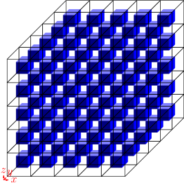
((a)) ((b))

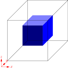
Fig. 5: (a) A whole domain $\Omega$ of heterogenous materials with a periodic microstructure; (b) the reference cell $Q=(0,1)^{3}$.

To determine the initial wave function $\Psi_{0}(\mathbf{x})$, we need to solve the time-independent Schrödinger equation. We take the wave function of the ground state as the initial wave function $\Psi_{0}(\mathbf{x})$ of the Maxwell-Schrödinger system (89). For more details, see [56].

In order to demonstrate the numerical accuracy of the present method, the exact solution $(\Psi^{\varepsilon}(\mathbf{x},t),\mathbf{E}^{\varepsilon}(\mathbf{x},t))$ of Maxwell-Schrödinger system (89) must be available. Since the elements of the coefficient matrices $(a_{ij}(\frac{\displaystyle\mathbf{x}}{\displaystyle\varepsilon}))$ and $(\mu_{ij}(\frac{\displaystyle\mathbf{x}}{\displaystyle\varepsilon}))$ are discontinuous, in general, it is an extremely difficult task or even impossible to obtain the exact solution. Here, we replace the exact solution $(\Psi^{\varepsilon}(\mathbf{x},t),\mathbf{E}^{\varepsilon}(\mathbf{x},t))$ by the numerical solution in a very fine mesh and at a small time step. It should be emphasized that this step is not necessary in the real applications. The computational costs for solving the Schrödinger equation and the Maxwell’s equations are listed in Table 1 and Table  2, respectively. The time step $\Delta t=0.0025$.

Table 1: Comparison of computational costs for solving the Schrödinger equation

	original problem	cell problems	homogenized equation
Dof	2478213	180135	76410
Number of elements	13573655	1034688	403590

Table 2: Comparison of computational costs for solving the Maxwell’s equations

	original problem	cell problems	homogenized equations
Dof	16125013	1229702	486888
Number of elements	13573655	1034688	403590

For simplicity, without confusion $\rho^{\varepsilon}=N|\Psi^{\varepsilon}|^{2}$ and $\mathbf{E}^{\varepsilon}$ denote the numerical solutions of the density function and the electric field for the Maxwell-Schrödinger system (89) in a fine mesh and at a time step $\Delta t=0.0025$, respectively, which are regarded as the reference solutions of the problem (89). Here $\rho^{0}=N|\Psi^{0}|^{2}$ and $\mathbf{E}^{0}$ are respectively the numerical solutions of the density function and the electric field for the associated homogenized Maxwell-Schrödinger system in a coarse mesh and at a time step $\Delta t=0.0025$. $\rho_{1}^{\varepsilon}=N|\Psi_{1}^{\varepsilon}|^{2}$ and $\rho_{2}^{\varepsilon}=N|\Psi_{2}^{\varepsilon}|^{2}$ are the first-order and the second-order multiscale solutions of the density function, respectively. $\mathbf{E}^{\varepsilon,(1)}$ and $\mathbf{E}^{\varepsilon,(2)}$ are the first-order and the second-order multiscale solutions of the electric field, respectively. Set $e_{0}=\rho^{\varepsilon}-\rho^{0}$, $e_{1}=\rho^{\varepsilon}-\rho_{1}^{\varepsilon}$, $e_{2}=\rho^{\varepsilon}-\rho_{2}^{\varepsilon}$, $\mathbf{e}_{0}=\mathbf{E}^{\varepsilon}-\mathbf{E}^{0}$, $\mathbf{e}_{1}=\mathbf{E}^{\varepsilon}-\mathbf{E}^{\varepsilon,(1)}$, $\mathbf{e}_{2}=\mathbf{E}^{\varepsilon}-\mathbf{E}^{\varepsilon,(2)}$. For convenience, we introduce the following notation. $\|\rho\|_{0}=\|\rho\|_{L^{2}(0,T;\/L^{2}(\Omega))}$, $\|\rho\|_{1}=\|\rho\|_{L^{2}(0,T;\/H^{1}(\Omega))}$, $\|\mathbf{E}\|_{(0)}=\|\mathbf{E}\|_{L^{2}(0,T;\/(L^{2}(\Omega))^{3})}$, $\|\mathbf{E}\|_{(1)}=\|\mathbf{E}\|_{L^{2}(0,T;\/\mathbf{H}(\mathbf{curl};\Omega))}$.

The computational results for the density function and the electric field in Example 5.1 are illustrated in Table 3 and Table 4, respectively.

Table 3: The computational results for the density function in Example 5.1

	$\frac{\|e_{0}\|_{0}}{\|\rho^{\varepsilon}\|_{0}}$	$\frac{\|e_{1}\|_{0}}{\|\rho^{\varepsilon}\|_{0}}$	$\frac{\|e_{2}\|_{0}}{\|\rho^{\varepsilon}\|_{0}}$	$\frac{\|e_{0}\|_{1}}{\|\rho^{\varepsilon}\|_{1}}$	$\frac{\|e_{1}\|_{1}}{\|\rho^{\varepsilon}\|_{1}}$	$\frac{\|e_{2}\|_{1}}{\|\rho^{\varepsilon}\|_{1}}$
Case 5.1.1	0.021350	0.012342	0.005139	0.224995	0.125434	0.036561
Case 5.1.2	0.031112	0.024987	0.005740	0.314168	0.248844	0.041702
Case 5.1.3	0.073949	0.071766	0.012427	0.536015	0.516680	0.081628

Table 4: The computational results for the electric field in Example 5.1

	$\frac{\|\mathbf{e}_{0}\|_{(0)}}{\|\mathbf{E}^{\varepsilon}\|_{(0)}}$	$\frac{\|\mathbf{e}_{1}\|_{(0)}}{\|\mathbf{E}^{\varepsilon}\|_{(0)}}$	$\frac{\|\mathbf{e}_{2}\|_{(0)}}{\|\mathbf{E}^{\varepsilon}\|_{(0)}}$	$\frac{\|\mathbf{e}_{0}\|_{(1)}}{\|\mathbf{E}^{\varepsilon}\|_{(1)}}$	$\frac{\|\mathbf{e}_{1}\|_{(1)}}{\|\mathbf{E}^{\varepsilon}\|_{(1)}}$	$\frac{\|\mathbf{e}_{2}\|_{(1)}}{\|\mathbf{E}^{\varepsilon}\|_{(1)}}$
Case 5.1.1	0.124387	0.079315	0.039245	1.147215	1.036499	0.793641
Case 5.1.2	0.166034	0.159700	0.067750	1.595115	1.239791	0.850183
Case 5.1.3	0.325069	0.321475	0.129570	2.719812	2.213347	0.889329

The evolution of the relative errors of the density function in $L^{2}(\Omega)$-norm and in $H^{1}(\Omega)$-norm with respect to time t in Case 5.1.1 is displayed in Fig. 6. The evolution of the relative errors of the electric field in $(L^{2}(\Omega))^{3}$-norm and in $\mathbf{H}(\mathbf{curl};\Omega)$-norm with respect to time t in Case 5.1.2 is illustrated in Fig. 7.

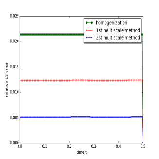
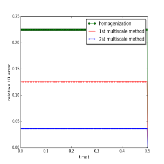
Fig. 6: Evolution of relative errors of the density function in the$\;L^{2}(\Omega)$-norm (left) and in the $\;H^{1}(\Omega)$-norm (right) in Case 5.1.1.

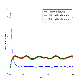
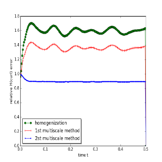
Fig. 7: Evolution of relative errors of the electric field in the$\;(L^{2}(\Omega))^{3}$-norm (left) and in the $\;\mathbf{H}(\mathbf{curl};\Omega)$-norm (right) in Case 5.1.2.

The computational results based on the homogenization method, the first-order and the second-order multiscale methods for the density function and the electric field on the intersection $x_{3}=0.45$ and at $T=0.3$ in Case 5.1.1, 5.1.2 and 5.1.3 are shown in Figs. 8, 9 and 10, respectively.

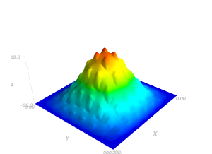
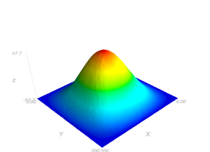
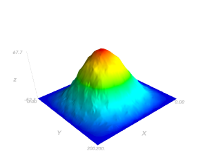
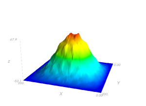
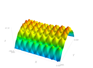
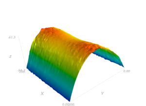
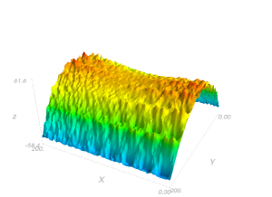
(a) (b) (c) (d) (e) (f) (g) (h)

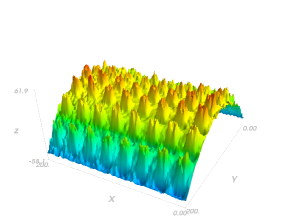
Fig. 8: Case 5.1.1: the density function and the first component of the electric field on the intersection $x_{3}=0.45$ and at $T=0.3$. (a) the reference solution $\rho^{\varepsilon}(\mathbf{x},t)$ in a fine mesh;  (b) the homogenized solution $\rho^{0}(\mathbf{x},t)$ in a coarse mesh;  (c) the first-order multiscale solution $\rho_{1}^{\varepsilon}(\mathbf{x},t)$;   (d)the second-order multiscale solution $\rho_{2}^{\varepsilon}(\mathbf{x},t)$;  (e) the reference solution $\mathbf{E}^{\varepsilon}(\mathbf{x},t)$ in a fine mesh;  (f) the homogenized solution $\mathbf{E}^{0}(\mathbf{x},t)$ in a coarse mesh;   (g) the first-order multiscale solution $\mathbf{E}^{\varepsilon,(1)}(\mathbf{x},t)$;  (h) the second-order multiscale solution $\mathbf{E}^{\varepsilon,(2)}(\mathbf{x},t)$. The time step $\Delta t=0.0025$.

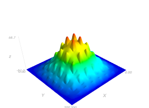
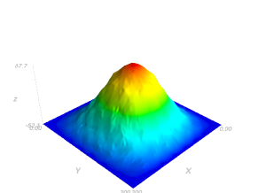
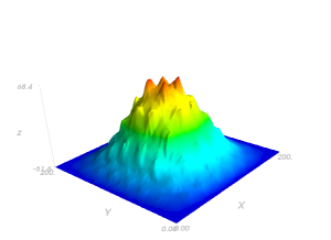
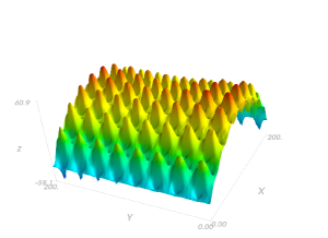
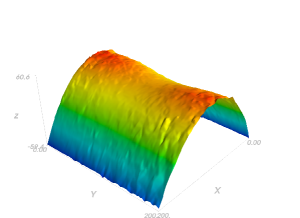
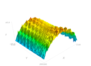
(a) (b) (c) (d) (e) (f) (g) (h)

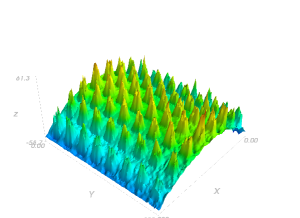
Fig. 9: Case 5.1.2: the density function and the second component of the electric field on the intersection $x_{3}=0.45$ and at $T=0.3$. (a) the reference solution $\rho^{\varepsilon}(\mathbf{x},t)$ in a fine mesh;  (b) the homogenized solution $\rho^{0}(\mathbf{x},t)$ in a coarse mesh;  (c) the first-order multiscale solution $\rho_{1}^{\varepsilon}(\mathbf{x},t)$;   (d)the second-order multiscale solution $\rho_{2}^{\varepsilon}(\mathbf{x},t)$;  (e) the reference solution $\mathbf{E}^{\varepsilon}(\mathbf{x},t)$ in a fine mesh;  (f) the homogenized solution $\mathbf{E}^{0}(\mathbf{x},t)$ in a coarse mesh;   (g) the first-order multiscale solution $\mathbf{E}^{\varepsilon,(1)}(\mathbf{x},t)$;  (h) the second-order multiscale solution $\mathbf{E}^{\varepsilon,(2)}(\mathbf{x},t)$. The time step $\Delta t=0.0025$.

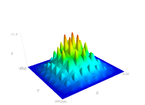
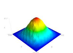
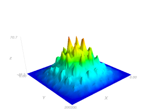
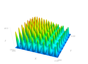
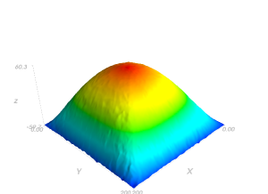
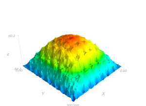
(a) (b) (c) (d) (e) (f) (g) (h)

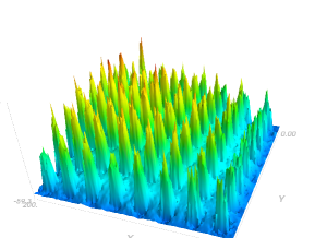
Fig. 10: Case 5.1.3: the density function and the third component of the electric field on the intersection $x_{3}=0.45$ and at $T=0.3$. (a) the reference solution $\rho^{\varepsilon}(\mathbf{x},t)$ in a fine mesh;  (b) the homogenized solution $\rho^{0}(\mathbf{x},t)$ in a coarse mesh;  (c) the first-order multiscale solution $\rho_{1}^{\varepsilon}(\mathbf{x},t)$;   (d)the second-order multiscale solution $\rho_{2}^{\varepsilon}(\mathbf{x},t)$;  (e) the reference solution $\mathbf{E}^{\varepsilon}(\mathbf{x},t)$ in a fine mesh;  (f) the homogenized solution $\mathbf{E}^{0}(\mathbf{x},t)$ in a coarse mesh;   (g) the first-order multiscale solution $\mathbf{E}^{\varepsilon,(1)}(\mathbf{x},t)$;  (h) the second-order multiscale solution $\mathbf{E}^{\varepsilon,(2)}(\mathbf{x},t)$. The time step $\Delta t=0.0025$.

 Example 5.2.

We consider the Maxwell-Schrödinger system (89) with rapidly oscillating discontinuous coefficients. Note that there is the exchange-correlation potential in (89) and we take $V_{xc}[\rho^{\varepsilon}]=-{(3\rho^{\varepsilon})}^{1/3}$. Let

$$\mbox{\bf Case 5.2.}\,\,\,a_{ij}(\frac{\displaystyle\mathbf{x}}{\displaystyle\varepsilon})=\left\{\begin{array}[]{l}0.025\delta_{ij},\quad\rm{in\,each\,cube}\\ \delta_{ij},\quad\rm{others}\end{array}\right.\quad\mu_{ij}(\frac{\displaystyle\mathbf{x}}{\displaystyle\varepsilon})=\left\{\begin{array}[]{l}\delta_{ij},\quad\rm{in\,each\,cube}\\ 0.01\delta_{ij},\quad\rm{others}.\end{array}\right.$$

The others are the same as those in Example 5.1.

The computational procedures in Example 5.2 are the same as those in Example 5.1 except that we have to solve the Schrödinger equation by the self-consistent iterative method. The numerical results are listed in Table 5 and Table 6, respectively.

Table 5: The computational results for the density function in Example 5.2

	$\frac{\|e_{0}\|_{0}}{\|\rho^{\varepsilon}\|_{0}}$	$\frac{\|e_{1}\|_{0}}{\|\rho^{\varepsilon}\|_{0}}$	$\frac{\|e_{2}\|_{0}}{\|\rho^{\varepsilon}\|_{0}}$	$\frac{\|e_{0}\|_{1}}{\|\rho^{\varepsilon}\|_{1}}$	$\frac{\|e_{1}\|_{1}}{\|\rho^{\varepsilon}\|_{1}}$	$\frac{\|e_{2}\|_{1}}{\|\rho^{\varepsilon}\|_{1}}$
Case 5.2	0.058699	0.055766	0.011276	0.479818	0.451818	0.067282

Table 6: The computational results for the electric field in Example 5.2

	$\frac{\|\mathbf{e}_{0}\|_{(0)}}{\|\mathbf{E}^{\varepsilon}\|_{(0)}}$	$\frac{\|\mathbf{e}_{1}\|_{(0)}}{\|\mathbf{E}^{\varepsilon}\|_{(0)}}$	$\frac{\|\mathbf{e}_{2}\|_{(0)}}{\|\mathbf{E}^{\varepsilon}\|_{(0)}}$	$\frac{\|\mathbf{e}_{0}\|_{(1)}}{\|\mathbf{E}^{\varepsilon}\|_{(1)}}$	$\frac{\|\mathbf{e}_{1}\|_{(1)}}{\|\mathbf{E}^{\varepsilon}\|_{(1)}}$	$\frac{\|\mathbf{e}_{2}\|_{(1)}}{\|\mathbf{E}^{\varepsilon}\|_{(1)}}$
Case 5.2	0.195816	0.079736	0.040340	1.147757	1.037087	0.814140

The computational results based on the homogenization method, the first-order and the second-order multiscale methods for the density function and the electric field on the line $x_{1}=x_{2}=x_{3}$ at $T=0.4$ in Case 5.2 are displayed in Fig. 11. The evolution of relative error in $L^{2}$ norm of the multiscale solutions of the density function and the electric field is illustrated in Fig. 12.

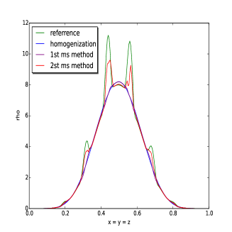
(a) (b)

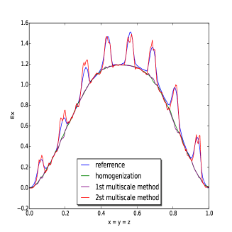
Fig. 11: (a) The density function on the line $x_{1}=x_{2}=x_{3}$ at time $T=0.4$ in Case 5.2 ;  (b) The third component of the electric field on the line $x_{1}=x_{2}=x_{3}$ at time $T=0.4$ in Case 5.2 ;  

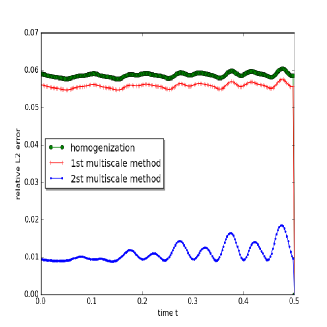
(a) (b)

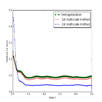
Fig. 12: (a) The evolution of relative error in $L^{2}$ norm of $\rho_{1}^{\varepsilon}$, $\rho_{2}^{\varepsilon}$ and $\rho^{0}$ in Case 5.2.  (b)The evolution of relative error in $L^{2}$ norm of $\mathbf{E}^{\varepsilon,(1)}$, $\mathbf{E}^{\varepsilon,(2)}$ and $\mathbf{E}^{0}$ in Case 5.2.

 Remark 5.1.

The comparison of computational costs listed in Tables 1 and 2 clearly shows that the multiscale asymptotic method provides a tremendous saving in computing resource, in particular, for a sufficiently small periodic parameter $\varepsilon>0$.

 Remark 5.2.

From the results reported in Example 5.1 (also see Tables 3 and 4), if there is a sharp difference between materials for the coefficient matrices $(a_{ij}(\frac{\displaystyle\mathbf{x}}{\displaystyle\varepsilon}))$ and $(\mu_{ij}(\frac{\displaystyle\mathbf{x}}{\displaystyle\varepsilon}))$, the homogenization method and the first-order multiscale method fail to provide satisfactory results. The second-order multiscale approach, however, is capable of producing accurate numerical solutions for the density function $\rho^{\varepsilon}$ and the electric field $\mathbf{E}^{\varepsilon}(\mathbf{x},t)$. The numerical results reported in Example 5.2 clearly shows that the second-order corrector terms are crucial in the proposed multiscale algorithm too.

 Remark 5.3.

The Maxwell’s equations and the Schrödinger equation can also be coupled through the vector potential $\mathbf{A}$ and the scalar potential $\varphi$ instead of $\hat{V}(\mathbf{x},t)=-\mathbf{E}(\mathbf{x},t)\cdot\widehat{\bm{\zeta}}$, which is called “length gauge”. Ohnuki et al. [39] verified theoretically and numerically that in the long-wavelength approximation, the length gauge is equivalent to the $\mathbf{A}-\varphi$ method.

Acknowledgments

The authors wish to thank Prof. Linbo Zhang, Prof.Zhiming Chen and Prof. Tao Cui for their help. The use of the PHG computing platform for numerical simulations is particularly acknowledged.

References

- [1] I. Ahmed and E. Li, Simulation of plasmonics nanodevices with coupled Maxwell and schrödinger equations using the FDTD method, Advanced Electromagnetics, 1(1)(2012): pp. 76–83.
- [2] G. Allaire and A. Piatnitski, Homogenization of the Schrödinger equation and effective mass theorems, Commun. Math. Phys., 258(1)(2005): pp. 1–22.
- [3] R.Beck, R.Hiptmair, R.H.W.Hoppe and B.Wohlmuth, Residual based on a posteriori estimates for eddy current computation, M2AN Math. Modeling and Numer.Anal., (2000), 34: 159–182.
- [4] V. Benci and D. Fortunato, Variational Methods in Nonlinear Field Equations: Solitary Waves, Hylomorphic Solitons and Vertices, Springer-Verlag, Berlin, 2014.
- [5] A. Bensoussan, J.L. Lions and G. Papanicolaou, Asymptotic Analysis for Periodic Structures, North-Holland, Amsterdam, 1978.
- [6] A. Bossavit, G. Griso, and B. Miara, Modelling of periodic electromagnetic structures bianisotropic materials with memory effects, J. Math. Pures Appl., 84 (2005), pp. 819–850.
- [7] L.Q. Cao and J.Z. Cui, Asymptotic expansions and numerical algorithms of eigenvalues and eigenfunctions of the Dirichlet problem for second order elliptic equations in perforated domains, Numer. Math., 96(3)(2004): pp. 525–581.
- [8] L.Q. Cao, J.L. Luo and C.Y. Wang, Multiscale analysis and numerical algorithm for the Schrödinger equations in heterogeneous media, Appl. Math. Comput., 217(2010): pp. 3955–3973.
- [9] L.Q. Cao, Y. Zhang, W. Allegretto, and Y.P. Lin, Multiscale asymptotic method for Maxwell’s equations in composite materials, SIAM J. Numer. Anal.,47(6) (2010), pp. 4257–4289.
- [10] L.Q. Cao, K.Q. Li, J.L. Luo and Y.S. Wong, A multiscale approach and a hybrid FE-FDTD algorithm for 3D time-dependent Maxwell’s equations in composite materials, Multiscale Model. & Simul., 13(4) (2015), pp. 1446-1477.
- [11] H. Chen, X. Gong and A. Zhou A, Numerical approximations of a nonlinear eigenvalue problem and applications to a density functional model, Math. Methods in the Appl. Sci., 33(14)(2010): pp. 1723–1742.
- [12] H. Chen, L. He and A. Zhou, Finite element approximations of nonlinear eigenvalue problems in quantum physics, Comput. Methods in Appl. Mech. and Engng., 200(21)(2011): pp. 1846–1865.
- [13] Z.Chen, L.Wang and W.Zheng, An adaptive multilevel method for time-harmonic Maxwell equations with sigularities, SIAM J.Sci. Comput., 29(2007): pp. 118–138.
- [14] D. Cioranescu and P. Donato, Introduction to Homogenization, Oxford University Press, New York, 1999.
- [15] T.C. Cohen, R.J. Dupont and C. Crynberg, Atom-Photon Interactions: Basic Processes and Applications, Wiley-VCH, Weinheim, 2004.
- [16] M. Costabel, M. Dauge and S. Nicaise, Sigularities of Maxwell interface problems, M2AN Math. Model Numer. Anal., 33(3)(1999):pp. 627–649.
- [17] M. Costabel and M. Dauge, Singularities of electromagnetic fields in polyhedral domains, Arch. Rational Mech. Anal., 151(2000): pp. 221–276.
- [18] C. Delerue and M. Lannoo, Nanostructures, Theory and Modeling, Springer-Verlag, Berlin, 2004.
- [19] G. Duvaut and J.L. Lions, Inequalities in Mechanics and Physics, Springer-Verlag, New York, 1976.
- [20] Z.F. Ezawa, Quantum Hall Effects: Recent Theoretical and Experimental Developments, Third Edition, World Scientific, Singapore, 2013.
- [21] D. Gilbarg and N. Trudinger, Elliptic Partial Differential Equations of Second Order, 2nd ed., Springer-Verlag, Berlin, New York, 1983.
- [22] J. Ginibre and G. Velo, Long range scattering and modified wave operators for the Maxwell-Schrödinger system I. The case of vanishing asymptotic magnetic field, Commun. Math. Phys., 236(2003): pp. 395–448.
- [23] Y. Guo, K. Nakamitsu and W. Strauss, Global finite-energy solutions of the Maxwell-Schrödinger system, Commun. Math. Phys., 170(1995): pp. 181-196.
- [24] T.P. Hamilton and P. Pulay, Direct inversion in the iterative subspace (DIIS) optimization of open-shell, excitedstate, and small multiconfiguration SCF wave functions, J. Chem. Phys., 84(10)(1986): pp. 5728–5734.
- [25] P. Harrison, Quantum Wells, Wires, and Dots, John Wiley & Sons, Ltd. Press, 2000.
- [26] X. Hu and W. Yang, Accelerating self-consistent field convergence with the augmented Roothaan Hall energy function, J. Chem. Phys., 132(5)(2010): pp. 054109-.
- [27] V.V. Jikov, S.M. Kozlov and O.A. Oleinik, Homogenization of Differential Operators and Integral Functionals, Springer-Verlag, Berlin, 1994.
- [28] H.-Chr. Kaiser and J. Gehberg, About a stationary Schrodinger-Poisson system with Kohn-Sham potential in a bounded two- or three-dimensional domain, Nonlinear Analysis, 41(2000), pp. 33–72.
- [29] Y.Y. Li and M. Vogelius, Gradient estimates for solutions to divergence form elliptic equations with discontinuous coefficients, Arch. Rational Mech. and Anal., 153(2)(2000): pp. 91–151.
- [30] K. Lopata and D. Neuhauser, Multiscale Maxwell-Schrödinger modeling: A split field finite-difference time-domain approach to molecular nanopolaritonics, J. Chem. Phys., 130(10)(2009): pp. 104707-.
- [31] E. Lorin, S. Chelkowski and A.D. Bandrauk, A numerical Maxwell-Schrödinger model for intense laser-matter interaction and propagation, Comput. Phys. Comm., 177(12)(2007): pp. 908–932.
- [32] E. Lorin and A.D. Bandrauk, Efficient and accurate numerical modeling of a micro-macro nonlinear optics model for intense and short laser pulses, J. Comput. Sci., 3(3)(2012): pp. 159–168.
- [33] R.M. Martin, Electronic Structure, Basic Theory and Practical Methods, Cambridge University Press, New York, 2004.
- [34] P. Monk, Finite Element Methods for Maxwell’s Equations , Clarendon press, Oxford, 2003.
- [35] K. Nakamitsu and M. Tsutsumi, The Cauchy problem for the coupled Maxwell-Schródinger equations, J. Math. Phys., 27(1)(1986): pp. 211–216.
- [36] M. Nakamura and T. Wada, Local well-posedness for the Maxwell-Schrödinger equation, Mathematische Annalen, 332(3)(2005): pp. 565–604.
- [37] M. Nakamura and T. Wada, Global existence and uniqueness of solutions to the Maxwell-Schrödinger equations, Commun. Math. Phys., 276(2)(2007): pp. 315–339.
- [38] J.C. Ndlec, Mixed finite elements in , Numer.Math., 35(1980): pp. 315–341.
- [39] S. Ohnuki et al., Coupled analysis of Maxwell-schrödinger equations by using the length gauge: harmonic model of a nanoplate subjected to a 2D electromagnetic field, Intern. J. of Numer. Model.: Electronic Networks, Devices and Fields, 26(6)(2013): pp. 533–544.
- [40] O.A. Oleinik, A.S. Shamaev and G.A. Yosifian, Mathematical Problems in Elasticity and Homogenization, North-Holland, Amsterdam, 1992.
- [41] L. Pierantoni, D. Mencarelli and T. Rozzi, A new 3-D transmission line matrix scheme for the combined Schrödinger-Maxwell problem in the electronic/electromagnetic characterization of nanodevices, IEEE Transactions on Microwave Theory and Techniques, 56(3)(2008): pp. 654–.
- [42] P. Pulay, Convergence acceleration of iterative sequences: The case of SCF iteration, Chem. Phys. Letters, 73(2)(1980): pp. 393–398.
- [43] S.M. Reimann and M. Manninen, Electronic structure of quantum dots, Rev. of Modern Phys., 74(4)(2002): pp. 1283–.
- [44] E. Sanchez-Palencia, Non-Homogeneous Media and Vibration Theory, Springer-Verlag, Berlin, Heidelberg, New York, 1980.
- [45] S.A. Sato and K. Yabana, Maxwell+ TDDFT multi-scale simulation for laser-matter interactions, Adv. Simul. Sci. Engng., 1(2014): pp. 98–110.
- [46] W. Schäfer and M. Wegener, Semiconductor Optics and Transport Phenomena, Springer-Verlag, Berlin, 2011.
- [47] A. Shimomura, Modified wave operator for Maxwell-Schrödinger equations in three space dimensions, Ann. Henri Poincaré, 4(2003): pp. 661–683.
- [48] Y. Tsutsumi, Global existence and asymptotic behavior of solutions for the Maxwell-Schrödinger equations in three space dimensions, Commun. Math. Phys., 151(3)(1993): pp. 543–576.
- [49] P. Turati and Y. Hao, A FDTD solution to the Maxwell-Schrödinger coupled model at the microwave range, Electromagnetics in Advanced Applications (ICEAA), 2012 International Conference on. IEEE, 2012: pp. 363–366.
- [50] C.A. Ullrich, Semiconductor Nanostructures, Lect. Notes Phys. 706: pp. 271–285, 2006.
- [51] T. Wada, Smoothing effects for Schrödinger equations with electro-magnetic potentials and applications to the Maxwell-Schrödinger equations, J. Functional Analysis, 263(2012): pp. 1-24.
- [52] N. Wellander, Homogenization of the Maxwell equations. Case I. Linear theory, Appl. Math., 46 (2001), pp. 29–51.
- [53] N. Wellander, Homogenization of the Maxwell equations. Case II. Nonlinear conductivity, Appl. Math., 47 (2002), pp. 255–283.
- [54] N. Wellander and G. Kristensson, Homogenization of the Maxwell equations at fixed frequency, SIAM J. Appl. Math., 64 (2003), pp. 170–195.
- [55] K. Yabana, T. Sugiyama, Y. Shinohara, et al., Time-dependent density functional theory for strong electromagnetic fields in crystalline solids, Phys. Rev. B, 85(4)(2012): pp. 045134–.
- [56] L.Zhang, L.Q. Cao and J.L. Luo, Multiscale analysis and computation for a stationary Schröinger-Poisson system in heterogeneous nanostructures, Multiscale Model. & Simul., 12(4)(2014): pp. 1561–1591.
- [57] Y. Zhang Y, L.Q. Cao and Y.S. Wong, Multiscale computations for 3D time-dependent Maxwell’s equations in composite materials, SIAM J. Sci. Comput., 32(5)(2010): pp. 2560–2583.
- [58] Y. Zhang, L.Q. Cao, W. Allegretto, and Y.P. Lin, Multiscale numerical algorithm for 3-D Maxwell’s equations with memory effects in composite materials, Intern. J. Numer. Anal. and Modeling, Ser. B, 1(2010), pp. 2560–2583.