A Logician’s View of Graph Polynomials

Abstract

Graph polynomials are graph parameters invariant under graph isomorphisms which take values in a polynomial ring with a fixed finite number of indeterminates. We study graph polynomials from a model theoretic point of view. In this paper we distinguish between the graph theoretic (semantic) and the algebraic (syntactic) meaning of graph polynomials. Graph polynomials appear in the literature either as generating functions, as generalized chromatic polynomials, or as polynomials derived via determinants of adjacency or Laplacian matrices. We show that these forms are mutually incomparable, and propose a unified framework based on definability in Second Order Logic. We show that this comprises virtually all examples of graph polynomials with a fixed finite set of indeterminates. Finally we show that the location of zeros and stability of graph polynomials is not a semantic property. The paper emphasizes a model theoretic view. It gives a unified exposition of classical results in algebraic combinatorics together with new and some of our previously obtained results scattered in the graph theoretic literature.

url]http://www.cs.technion.ac.il/ janos

url]http://forsyte.at/people/kotek

1 Introduction

This paper gives a logician’s view of some aspects of graph polynomials. A short version was given as an invited lecture by the first author at WOLLIC 2016, [63].

A graph $G=(V(G),E(G))$ is given by the set of vertices $V(G)$ and a symmetric edge-relation $E(G)$. We denote by $n(G)$ the number of vertices, by $m(G)$ the number of edges, by $k(G)$ the number of connected components of a graph $G$, and by $\mathcal{G}$ the class of finite graphs.

Graph polynomials are graph invariants with values in a polynomial ring $\mathcal{R}$, usually ${\mathbb{Z}}[\mathbf{X}]$ with $\mathbf{X}=(X_{1},\ldots,X_{\ell})$. Let ${\mathbf{P}}(G;\mathbf{X})$ be a graph polynomial of the form

$${\mathbf{P}}(G;\mathbf{X})=\sum_{i_{1},\ldots,i_{\ell}=0}^{d(G)}c_{i_{1},\ldots,i_{\ell}}(G)X_{1}^{i_{1}}\cdot\ldots\cdot X_{\ell}^{i_{\ell}},$$

where $\mathbf{X}=(X_{1},\ldots,X_{\ell})$, $d(G)$ is a graph parameter with non-negative integers as its values, and

$$c_{i_{1},\ldots,i_{\ell}}(G):i_{1},\ldots,i_{\ell}\leq d(G)$$

are integer valued graph parameters.

Definition 1.1.

A graph polynomial ${\mathbf{P}}(G;\mathbf{X})$ is computable if

1. ${\mathbf{P}}(G;\mathbf{X})$ is a Turing computable function, and additionally,

2. the range of ${\mathbf{P}}(G;\mathbf{X})$, the set

   $$\{p(\mathbf{X})\in{\mathbb{Z}}[\mathbf{X}]:\mbox{ there is a graph }G\mbox{ with }{\mathbf{P}}(G;\mathbf{X})=p(\mathbf{X})\}$$

   is Turing decidable.

The second condition is needed to make Theorem 2.2 work.

Graph polynomials have been studied for the last hundred years, since G. Birkhoff introduced his chromatic polynomial in [11]. This was generalized by H. Whitney in the 1930ties, [79] and led to the Tutte polynomial, also called the dichromate or the Tutte-Whitney polynomial. For a history see [23]. Motivated by questions in theoretical chemistry, the characteristic polynomial and the matching polynomial of graphs were introduced, and studied intensively, [40, 37, 73, 5, 6, 41]. In the last 30 years many more graph polynomials appeared in the literature. The abundance of graph polynomials which appear in the more recent literature leads to various questions:

• How to compare graph polynomials?

• What kind of information may be extracted from a graph polynomial about its underlying graph?

• Are there any normal forms of graph polynomials?

Ten years ago B. Zilber and the first author have discovered a connection between model theory and graph polynomials, [65, 51]. In [64] we introduced the distinction between syntactic and semantic properties of graph polynomials. In logic two formulas are semantically (logically) equivalent if they have the same models, in other words, if they do not distinguish between two models. Syntactic properties of formulas refer to properties of the string which is the formula. Prenex normal form is a syntactic property. Semantic properties of a formula are properties of the class of models of this formula shared by the class of models of logically equivalent formulas. For graph polynomials $P(G;\mathbf{X})$ syntactic properties are properties of the particular polynomials $P(G;\mathbf{X})$ for each $G$, whereas two graph polynomials are semantically equivalent if they do not distinguish between any pair of graphs, or graphs with the same number of vertices, edges and connected components. Our discussion in the above and subsequent papers, was mostly addressed the graph theory community. This paper is written for the logically minded and is a continuation of our analysis of notions used in the literature on graph polynomials.

1.1 Why study graph polynomials?

The first graph polynomial, the chromatic polynomial, was introduced in 1912 by G. Birkhoff to study the Four Color Conjecture, [11]. The emergence of the Tutte polynomial can be seen as an attempt to generalize the chromatic polynomial, cf. [75, 12, 22]. The characteristic polynomial and the matching polynomial were introduced with applications from chemistry in mind, cf. [73, 5, 6, 14, 9]. Physicists study various partition functions in statistical mechanics, in percolation theory and in the study of phase transitions, cf. [67]. It turns out that many partition functions are incarnations of the Tutte polynomial. Another incarnation of the Tutte polynomial is the Jones polynomial in Knot Theory, [45] and again [12]. The various incarnations of the Tutte polynomial have triggered an interest in other graph polynomials. These graph polynomials are studied for various reasons:

• Graph polynomials can be used to distinguish non-isomorphic graphs. A graph polynomial is complete if it distinguishes all non-isomorphic graphs. The quest for a complete graph polynomial which is also easy to compute failed so far for two reasons. Either there were too many non-isomorphic graphs which could not be distinguished, and/or the proposed graph polynomial was more difficult to compute than just checking graph isomorphism.

• New graph polynomials may appear when we model behavior of physical, chemical or biological systems. The arguments whether a graph polynomial is interesting, depends on its success in predicting the behavior of the modeled systems. Also the particular choice of the representation is dictated by the modeling process. The fact that the modeled process gives, in this case, rise to a particular graph polynomial, is secondary, and the properties of the graph polynomial reflect more properties of the physical or chemical process modeled, than properties of the underlying graph.

• New graph polynomials are also studied as part of graph theory proper. Here one is interested in the interrelationship between various graph parameters without particular applications in mind. A graph polynomial is considered interesting from a graph theoretic point of view, if many graph parameters can be (easily) derived from it.

• Graph polynomials are sometimes studied as a way of generating families of polynomials, irrespective of their graph theoretic meaning. H. Wilf, [80] asked the question how to characterize the polynomials which do occur as instances of chromatic polynomials of graphs as a family of polynomials. We have addressed this approach to graph polynomials in [48].

This paper deals only with the graph theoretic and logical aspects of graph polynomials, discarding the graph isomorphism problem and discarding the modeling of systems describing phenomena in the natural sciences. We ultimately ask the question: When is a newly introduced graph polynomial interesting from a graph theoretic or logical point of view and deserves to be studied, and what aspects are more rewarding in this study than others. In particular, in the last part of this paper, we scrutinize the role of the location of the roots of specific graph polynomials in terms of other graph theoretic properties.

1.2 Why not just sequences of integers rather than polynomials?

A graph polynomial $P(G;\mathbf{X})$ is uniquely determined by the sequences of its coefficients. In practice these coefficients were usually chosen in a uniform way having some combinatorial interpretation. The function which associates such a sequence with a polynomial is rather artificial. Whether the coefficient $c_{i}$ is associated with $X^{i}$ or some other monomial $X^{j}$ or polynomial $g_{i}(X)$, or even a function $f_{i}(X)$ which is not a polynomial in $X$ will depend on the graph theoretic question one wants to study. Historically, for the last hundred years, polynomials were used. After it was discovered that the Four-Color-Conjecture can be formulated as a problem about the chromatic polynomial, one is easily tempted to look for other graph theoretic statements which be formulated in a similar way. The abundance of such statements might make one believe that graph polynomials are a good choice for studying graph theoretical questions.

It is conceivable that other ways of studying the same sequences are equally interesting, but the fact is, that such investigations are absent from the literature. Maybe our analysis of the way graph polynomials arise in general will spur new lines of research, replacing graph polynomials by other algebraic or analytic formalisms.

1.3 Why $\mathrm{SOL}$-definability?

There are uncountably many graph polynomials if they are merely defined as graph invariants with values in a polynomial ring. We can impose more restrictions by imposing computability and, in an even more restrictive way, definability requirements. Imposing complexity theoretic restrictions poses some serious problems, and is studied in [59]. However, it is not the subject of this paper.

The earliest graph polynomials are the chromatic polynomial introduced in 1912, its generalization the Tutte polynomial, introduced in 1954 and the characteristic and matching polynomials introduced in the 1950ties. It is not right away obvious how to find a common generalization. The chromatic polynomial is a special case of a Harary polynomial (a generalization of the chromatic polynomial introduced by Harary [28], the matching polynomial is a special case of a generation function, and the characteristic polynomial is based on computing a determinant of some matrix associated with a graph.

In [55, 1, 51, 31] the class of graph polynomials definable in Second Order Logic ($\mathrm{SOL}$), is studied, which requires that $d(G)$ and $c_{\mathbf{\i}}(G)=c(G;\mathbf{\i})$, $\mathbf{\i}=(i_{1},\ldots,i_{\ell})$, are, even uniformly, definable in $\mathrm{SOL}$. With very few exceptions, the graph polynomials studied in the literature are $\mathrm{SOL}$-definable.

It turns out that the $\mathrm{SOL}$-definable graph polynomials are the smallest class of graph polynomials subject to some very natural closure properties which cover all the examples studied in the literature. On the other hand we show in Sections 5 that certain naturally defined graph polynomials (the domination polynomial and certain generalzed chromatic polynomials) cannot be written as generating fuctions or Harary polynomials.

We assume the reader is familiar with Finite Model Theory, cf. [21, 53]. The finite model theory of graph polynomials was developed in [57, 52, 51]. For the convenience of the reader it will summarized in Section 6.

Requiring that the graph polynomials are $\mathrm{SOL}$-definable also guarantees that their coefficients are the result of counting combinatorially meaningful $\mathrm{SOL}$-definable configurations in the underlying graph.

1.4 On the location of roots of graph polynomials

Up to this point we were mostly concerned with the logical presentation of graph polynomials and justified, why our formalism of $\mathrm{SOL}$-definable graph polynomial is an appropriate choice. A topic frequently studied in paper about graph polynomials is the location of the roots (zeroes) of $P(G;\mathbf{X})$ for a fixed graph $G$.

Given a univariate graph polynomial ${\mathbf{P}}(G;X)$ a complex number $z\in{\mathbb{C}}$ is a root of ${\mathbf{P}}$ if there is a graph $G$ such that $z$ is a root of ${\mathbf{P}}(G;X)$. Many results in the literature on graph polynomials deal with the location of its roots. For multivariate graph polynomials the corresponding question is formulated in terms of half-plane properties. The location of the zeroes is a good question to illustrate the difference between graph theoretic (semantic) and algebraic (syntactic) properties of graph polynomials. The last part of this paper shows that the location of roots is not a semantic property.

We first paraphrase the main results of [64]. These results are all of the form:

(*) Let $U$ be a subset of the complex numbers, such as the reals, an open disk, the lower or upper halfplane, or the complement thereof. Given a univariate $\mathrm{SOL}$-definable graph polynomial ${\mathbf{P}}(G;X)$, there exists a semantically equivalent $\mathrm{SOL}$-definable graph polynomial ${\mathbf{Q}}(G;X)$ with all its roots in $U$.

They show, in a precise sense, that the location of the roots of a univariate graph polynomial is not a semantic property. They are more of a normal form property: Every univariate $\mathrm{SOL}$-definable graph polynomial ${\mathbf{P}}(G;X)$ can be put into a semantically equivalent form with prescribed location of its roots.

The proofs in [64] have two parts: Finding ${\mathbf{Q}}(G;X)$, and showing that this ${\mathbf{Q}}(G;X)$ is $\mathrm{SOL}$-definable. Finding ${\mathbf{Q}}(G;X)$ often uses some “dirty trick” from analysis, whereas showing $\mathrm{SOL}$-definability, only sketched in [64], needs more efforts in the details.

In this paper we extend results of [64] to multivariate graph polynomials ${\mathbf{P}}(G;\mathbf{X})$. We show that various versions of the ”halfplane property” in higher dimensions of multivariate graph polynomials are also not semantic properties of the underlying graph in the sense of (*). This is interesting for two reasons: First, these halfplane properties were studied in the recent literature on graph polynomials, and, second, the proofs that the constructed ${\mathbf{Q}}(G;\mathbf{X})$ is $\mathrm{SOL}$-definable is much more complex. For the convenience of the logically minded reader we repeat many examples already discussed in [64]. Furthermore, we provide in this paper the details in proving $\mathrm{SOL}$-definability for the more difficult case of multivariate graph polynomials and the various halfplane properties.

1.5 Outline of the paper

In Section 2 we discuss the foundational aspects of comparing graph polynomials. In Section 3 we discuss different ways of representing graph polynomials and introduce the notion of semantic (graph theoretic) and syntactic (algebraic) properties of graph polynomials. In Section 4 we present the discussion of various notions of equivalence of graph polynomials based on their distinctive power which also is part of Section 5. In Section 6 we develop the framework of $\mathrm{SOL}$-definable graph polynomials. This summarizes the framework given in [52]. In Section 7 we discuss the location of zeros of graph polynomials. First, in Subsection 7.1, we review our previous results previously published in [64], which show that the location of roots of univariate graph polynomials is not a semantic property. Then, in Subsection 7.2, we look at the multivariate version of the location of roots, the various halfplane properties, also called stability properties, and prove that stability is also not a semantic property of multivariate graph polynomials. The discussion of stable polynomials is appears for the first time in this paper. Finally, in Section 8 we draw our conclusions and formulate several open problems.

2 How to compare graph polynomials?

Once the graph theorists started to study several graph polynomials, the need of comparing them naturally arises. We analyze two notions of equivalence which both occur implicitely in the literature in many papers. Authors will argue that their graph polynomial is different from other graph polynomials. They will argue that

• Some other graph polynomial is a special case of the newly studied graph polynomial.

• The newly introduced graph polynomial is incomparable to previously studied graph polynomials.

• The newly introduced graph polynomial is the most general graph polynomial withing a certain class of graph invariants.

By analyzing the literature we extracted two ways of comparison, d.p.- and s.d.p.-equivalence, which encompass all other notions used in various papers. This section discusses the basic properties of these notions. From a model-theoretic point of view, d.p.-equivalence is the more natural notion. However, most graph theoretic papers compare the behaviour of graph polynomials only on graphs with the same number of vertices, edges and connected components, which is captured by s.d.p.-equivalence.

For $\mathcal{R}\in\{{\mathbb{R}},{\mathbb{C}},{\mathbb{Z}}\}$ we denote by $\mathfrak{GP}_{\mathcal{R},r}$ the set of graph polynomials in $r$ indeterminates with coefficients in $\mathcal{R}$, and let $\mathbf{X}=(X_{1},\ldots,X_{r})$ be $r$ indeterminates. Let ${\mathbf{P}}(G)={\mathbf{P}}(G;\mathbf{X})$ and ${\mathbf{Q}}(G)={\mathbf{Q}}(G;\mathbf{X})$ be two graph polynomials.

The following statements appear frequently in the literature with the intended meaning, but without a general definition:

1. ${\mathbf{Q}}(G)$ is a substitution instance of ${\mathbf{P}}(G)$.

2. ${\mathbf{Q}}(G)$ and ${\mathbf{P}}(G)$ are really the same, up to a prefactor. For example the various versions of the Tutte polynomial are said to be the same up to a prefactor, [71], and the same holds for the various versions of the matching polynomial, [54].

3. ${\mathbf{Q}}(G)$ is at least as expressive than ${\mathbf{P}}(G)$.

4. The coefficients of ${\mathbf{P}}(G)$ can be determined, or even computed, from the coefficients of ${\mathbf{Q}}(G)$.

Usually these statements are understood to be uniform in the graphs $G$, but this uniformity can take various forms. In [64] we have given these statements precise meanings, and we have initiated the analysis of their relationship. In this paper we elaborate our approach from [64] further with the logic community in mind.

From a model theoretic point of view a graph property is a Boolean graph parameter. A closed formula in a logical formalism, say a fragment of $\mathrm{SOL}$, is a syntactic object. Its meaning is given by a graph property, i.e., a class of finite graphs closed under isomorphism. Two formulas are considered logically equivalent if they define the same property. In other words, two formulas are considered equivalent if they do not distinguish between two graphs. As Boolean graph parameters have only two possible values, two formulas are equivalent if, considered as graph parameters, they define the same function.

Let $\mathcal{R}$ be a possibly infinite ring. An $\mathcal{R}$-valued graph parameter is a function $f$ which maps a graph $G$ into an element $f(G)\in\mathcal{R}$. A graph polynomial ${\mathbf{P}}(G)$ is a graph parameter which takes values in a polynomial ring.

Graph parameters are coextensive if they define the same function. However, co-extensiveness seems to be too strong a property to compare graph parameters. For instance defining the size of a graph $G$ by its order $n(G)=|V(G)|$, or by $n^{\prime}(G)=2\cdot|V(G)|$, gives two non-coextensive graph parameters which still have the same information content in the following sense. For two $\mathcal{R}$-valued graph parameters $f$ and $g$, we say that $g$ is at least as distinctive as $f$, if for two graphs $G_{1},G_{2}$ $g$ does not distinguish between $G_{1}$ and $G_{2}$, i.e., $g(G_{1})=g(G_{2})$, then also $f$ does not distinguish between $G_{1}$ and $G_{2}$, i.e., $f(G_{1})=f(G_{2})$.

Graph theorists often compare the distinctive power of graph parameters on graphs which are not trivially distinguishable. Here trivially distinguishable refers to different order, size or number of components.

2.1 Equivalence of graph polynomials

Let ${\mathbf{P}}(G)$ be a graph polynomial. We say that two graphs $G,H$ are similar if they have the same number of vertices, edges and connected components. A graph parameter or a graph polynomial is a similarity function if it is invariant under graph similarity.

Two graphs $G,H$ are ${\mathbf{P}}$-equivalent if ${\mathbf{P}}(H;\mathbf{X})={\mathbf{P}}(G;\mathbf{X})$. ${\mathbf{P}}$ distinguishes between $G$ and $H$ if $G$ and $H$ are not ${\mathbf{P}}$-equivalent. Two graph polynomials ${\mathbf{P}}(G;\mathbf{X})$ and ${\mathbf{Q}}(G;\mathbf{Y})$ with $r$ and $s$ indeterminates respectively can be compared by their distinctive power on similar graphs: ${\mathbf{P}}(G;\mathbf{X})$ is at most as distinctive as ${\mathbf{Q}}(G;\mathbf{Y})$, ${\mathbf{P}}(G;\mathbf{X})\leq_{s.d.p}{\mathbf{Q}}(G;\mathbf{Y})$ if any two similar graphs $G,H$ which are ${\mathbf{Q}}$-equivalent are also ${\mathbf{P}}$-equivalent. ${\mathbf{P}}(G;\mathbf{X})$ and ${\mathbf{Q}}(G;\mathbf{Y})$ are s.d.p.-equivalent, ${\mathbf{P}}(G;\mathbf{X})\sim_{s.d.p}{\mathbf{Q}}(G;\mathbf{Y})$ if for any two similar graphs $G,H$ ${\mathbf{P}}$-equivalence and ${\mathbf{Q}}$-equivalence coincide. We can also compare graph polynomials on graphs without requiring similarity. In this case we say that a graph polynomial ${\mathbf{P}}$ is at most as distinctive as ${\mathbf{Q}}$, ${\mathbf{P}}\leq_{d.p.}{\mathbf{Q}}$, if for all graphs $G_{1}$ and $G_{2}$ we have that

$${\mathbf{Q}}(G_{1};\mathbf{Y})={\mathbf{Q}}(G_{2};\mathbf{Y})\mbox{ implies }{\mathbf{P}}(G_{1};\mathbf{X})={\mathbf{P}}(G_{2};\mathbf{X})$$

${\mathbf{P}}$ and ${\mathbf{Q}}$ are d.p.-equivalent iff both ${\mathbf{P}}\leq_{d.p.}{\mathbf{Q}}$ and ${\mathbf{Q}}\leq_{d.p.}{\mathbf{P}}$. D.p.-equivalence is stronger that s.d.p.-equivalence:

Lemma 2.1.

For any two graph polynomials ${\mathbf{P}}$ and ${\mathbf{Q}}$ we have: ${\mathbf{P}}\leq_{d.p.}{\mathbf{Q}}$ implies ${\mathbf{P}}\leq_{s.d.p.}{\mathbf{Q}}$.

A graph $G$ is ${\mathbf{P}}$-unique if for all graphs $G^{\prime}$ the polynomial identity ${\mathbf{P}}(G;\mathbf{X})={\mathbf{P}}(G^{\prime};\mathbf{X})$ implies that $G$ is isomorphic to $G^{\prime}$. As a graph invariant ${\mathbf{P}}(G;\mathbf{X})$ can be used to check whether two graphs are not isomorphic. For $P$-unique graphs $G$ and $G^{\prime}$ the polynomial ${\mathbf{P}}(G;\mathbf{X})$ can also be used to check whether they are isomorphic.

Our notion of similarity is extracted from the literature on graph polynomials: It is implicitly used frequently both in claims that two polynomials are “really the same”, or “the same up to a prefactor”. From a logical point of view one would rather define a more general notion: Let $\Sigma$ be a finite set of graph parameters. Two graphs $G,H$ are $\Sigma$-similar if they have the same values $s(G)=s(H)$ for all $s\in\Sigma$. It is easy, but currently of little use, to rewrite the definitions of various forms of equivalence of graph polynomials using $\Sigma$-similarity rather than similarity as we defined it in this paper.

Theorem 2.2.

1. ${\mathbf{P}}$ is at most as distinctive as ${\mathbf{Q}}$, ${\mathbf{P}}\leq_{d.p}{\mathbf{Q}}$, iff there is a function $F:{\mathbb{Z}}[\mathbf{Y}]\rightarrow{\mathbb{Z}}[\mathbf{X}]$ such that for every graph $G$ we have

   $${\mathbf{P}}(G;\mathbf{X})=F({\mathbf{Q}}(G;\mathbf{Y}))$$

2. ${\mathbf{P}}$ is at most as distinctive as ${\mathbf{Q}}$ on similar graphs, ${\mathbf{P}}\leq_{s.d.p}{\mathbf{Q}}$, iff there is a function $F:{\mathbb{Z}}[\mathbf{Y}]\times{\mathbb{Z}}^{3}\rightarrow{\mathbb{Z}}[\mathbf{X}]$ such that for every graph $G$ we have

   $${\mathbf{P}}(G;\mathbf{X})=F({\mathbf{Q}}(G;\mathbf{Y}),n(G),m(G),k(G))$$

3. Furthermore, both for d.p. and s.d.p., if both ${\mathbf{P}}$ and ${\mathbf{Q}}$ are computable, then $F$ is computable, too.

The equivalence in (ii) in Theorem 2.2 was first proved in [64]. For the convenience of the reader we repeat it below. Moreover, (iii) is new, and follows from our definition of computability of graph polynomials. We note here that (ii) is useful for proving d.p.-reducibility, whereas (i) is more useful to prove its negation. Theorem 2.2 shows that our definition of d.p.-equivalence of graph polynomials is mathematically equivalent to the definition proposed in [60].

Proof of Theorem 2.2(ii)-(iii).

(ii) $\Rightarrow$:
Let $S$ be a set of finite graphs and $s\in{\mathbb{Z}}[\mathbf{X}]$. For a graph polynomial ${\mathbf{P}}$ we define:

$${\mathbf{P}}[S]=\{s\in{\mathbb{Z}}[\mathbf{X}]:{\mathbf{P}}(G)=s\mbox{ for some }G\in S\}$$

$${\mathbf{P}}^{-1}(s)=\{G:{\mathbf{P}}(G)=s\}.$$

Now assume ${\mathbf{P}}(G;\mathbf{X})\preceq_{s.d.p.}{\mathbf{Q}}(G;\mathbf{Y})$.
If ${\mathbf{Q}}^{-1}(s)\neq\emptyset$, then for every $G_{1},G_{2}\in{\mathbf{Q}}^{-1}(s)$ we have ${\mathbf{Q}}(G_{1},\mathbf{Y})={\mathbf{Q}}(G_{2},\mathbf{Y})$, and therefore ${\mathbf{P}}(G_{1},\mathbf{X})={\mathbf{P}}(G_{2},\mathbf{X})$. Hence $P[{\mathbf{Q}}^{-1}(s)]=\{t_{s}\}$ for some $t_{s}\in{\mathbb{Z}}[\mathbf{X}]$. Now we define

$$F_{{\mathbf{P}},{\mathbf{Q}}}(s)=\begin{cases}t_{s}&{\mathbf{Q}}^{-1}(s)\neq\emptyset\\ s&\mbox{else}\end{cases}$$

$\Leftarrow$:
Assume there is a function $F:{\mathbb{Z}}[\mathbf{Y}]\rightarrow{\mathbb{Z}}[\mathbf{X}]$ such that for all graphs $G$ we have $F({\mathbf{Q}}(G))={\mathbf{P}}(G)$.

Now let $G_{1},G_{2}$ be similar graphs such that ${\mathbf{Q}}(G_{1})={\mathbf{Q}}(G_{2})$. Hence, $F({\mathbf{Q}}(G_{1}))=F({\mathbf{Q}}(G_{2}))$. Since for all $G$ we have $F({\mathbf{Q}}(G))={\mathbf{P}}(G)$, we get ${\mathbf{P}}(G_{1})={\mathbf{P}}(G_{2})$.

Proof of (iii): Now assume both ${\mathbf{P}}(G;\mathbf{X})$ and ${\mathbf{Q}}(G;\mathbf{Y})$ are computable. To see that $F$ is computable we note that it suffices, as in the proof of (i), to find an element $s$ in the range of ${\mathbf{Q}}$ and a graph $G_{s}$ such that ${\mathbf{Q}}(G_{s})=s$. The latter can be done since the range of ${\mathbf{Q}}$ is Turing decidable by Definition 1.1(ii). ∎

2.2 Examples of equivalent graph polynomials

Example 2.3.

Let $m_{k}(G)$ denote the number of $k$-matchings ($k$ many independent edges) of $G$. There are two versions of the univariate matching polynomial, [54]: The matching defect polynomial (or acyclic polynomial)

$$\mu(G;X)=\sum_{k=0}^{\lfloor\frac{n}{2}\rfloor}(-1)^{k}m_{k}(G)X^{n-2k},$$

and the matching generating polynomial

$$g(G;X)=\sum_{k=0}^{n}m_{k}(G)X^{k}.$$

The relationship between the two is given by

$$\mu(G;X)=\sum_{k=0}^{\lfloor\frac{n}{2}\rfloor}(-1)^{k}m_{k}(G)X^{n-2k}=X^{n}\sum_{k=0}^{\lfloor\frac{n}{2}\rfloor}(-1)^{k}m_{k}(G)X^{-2k}=$$

$$=X^{n}\sum_{k=0}^{\lfloor\frac{n}{2}\rfloor}m_{k}(G)((-1)\cdot X^{-2})^{k}=X^{n}\sum_{k=0}^{\lfloor\frac{n}{2}\rfloor}m_{k}(G)(-X^{-2})^{k}=X^{n}g(G;(-X^{-2}))$$

It follows that $g$ and $\mu$ are equally distinctive, and can be computed from each other by a simple substitution and multiplication of a factor which depends only on the number of vertices, edges and connected components. However, assume $G$ has no isolated vertices and $E_{n}$ is the graph without edges on $n$ vertices with $E_{0}=\emptyset$. Then $g(G;X)=g(G\sqcup E_{n};X)$ for all $n\in{\mathbb{N}}$, i.e., $g(G;X)$ is invariant under addition or removal of isolated vertices. However, this is not true for $\mu(G;X)$, which depends on the number of isolated vertices.

Example 2.4.

Let ${\mathbf{P}}(G;X)$ be a univariate graph polynomial with integer coefficients and

$${\mathbf{P}}(G;X)=\sum_{i=0}^{d(G)}a_{i}(G)X^{i}=$$

$$=\sum_{i=0}^{d(G)}b_{i}(G)X_{(i)}=$$

$$=\sum_{i=0}^{d(G)}c_{i}(G){X\choose i}=$$

$$=\prod_{i}^{d(G)}(X-z_{i})$$

where $X_{(i)}=X(X-1)\cdot\ldots\cdot(X-i+1)$ is the falling factorial function. We denote by $a{\mathbf{P}}(G)=(a_{0}(G),a_{1}(G),\ldots a_{d(G)})$, $b{\mathbf{P}}(G)=(b_{0}(G),b_{1}(G),\ldots b_{d(G)})$ and $c{\mathbf{P}}(G)=(c_{0}(G),c_{1}(G),\ldots c_{d(G)})$ the coefficients of these polynomial presentations and by $z{\mathbf{P}}(G)=(z_{1},\ldots,z_{d(G)})$ the roots of these polynomials with their multiplicities. We note that the four presentations of ${\mathbf{P}}(G;X)$ are all d.p.-equivalent.

Example 2.5.

Let $G=(V(G),E(G))$ be a loopless graph without multiple edges. Let $A_{G}$ be the adjacency matrix of $G$, $D_{G}$ the diagonal matrix with $(D_{G})_{i,i}=d(i)$, the degree of the vertex $i$, and $L_{G}=D_{G}-A_{G}$. In spectral graph theory two graph polynomials are considered, the characteristic polynomial of $G$, here denoted by $P_{A}(G;X)=\det(X\cdot\mathbb{I}-A_{G})$, and the Laplacian polynomial, here denoted by $P_{L}(G;X)=\det(X\cdot\mathbb{I}-L_{G})$. Here $\mathbb{I}$ denotes the unit element in the corresponding matrix ring. Here we show that the polynomials $P_{A}(G;X)$ and $P_{L}(G;X)$ are d.p.-incomparable. $G$ and $H$ in Figure 1 are similar. We have

$$P_{A}(G;X)=P_{A}(H;X)=(X-1)(X+1)^{2}(X^{3}-X^{2}-5X+1),$$

but $G$ has eight spanning trees, and $H$ has six. Therefore, $P_{L}(G;X)\neq P_{L}(H;X)$, as one can compute the number of spanning trees from $P_{L}(G;X)$. For more details, cf. [9, Exercise 1.9].

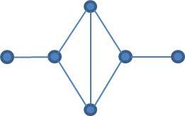
$G$                                     $H$

Figure 1: Similar graphs with different number of spanning trees

On the other hand, $G^{\prime}$ and $H^{\prime}$ in Figure 2 are similar, but $G^{\prime}$ is not bipartite, whereas, $H^{\prime}$ is.

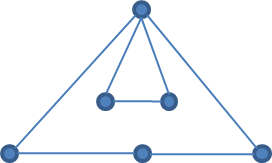
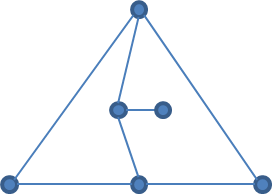
$G^{\prime}$                                     $H^{\prime}$

Figure 2: Similar graphs with different chromatic numbers

Hence $P_{A}(H^{\prime};X)\neq P_{A}(G^{\prime},X)$, but $P_{L}(H^{\prime};X)=P_{L}(G^{\prime};X)$. See, [9, Lemma 14.4.3].

Conclusion: The characteristic polynomial and the Laplacian polynomial are d.p.-incomparable. However, if restricted to $r$-regular graphs, they are d.p.-eqivalent, [9].

2.3 Prefactor equivalence

We recall that a graph parameter $f(G)$ with values in some function space $\mathbf{F}$ over some ring $\mathcal{R}$ is called a similarity function if for any two similar graphs $G,H$ we have that $f(G)=f(H)$. If $\mathbf{F}$ is a subset of the set of analytic functions we speak of analytic similarity functions.

If $\mathbf{F}$ is the polynomial ring ${\mathbb{Z}}[\mathbf{X}]$ with set of indeterminates $\mathbf{X}=(X_{1},\ldots X_{r})$, we speak of similarity polynomials. It will be sometimes useful to allow classes of functions spaces which are closed under reciprocals and inverses rather than just similarity polynomials.

Example 2.6.

Typical examples of similarity functions are

1. The nullity $\nu(G)=m(G)-n(G)+k(G)$ and the rank $\rho(G)=n(G)-k(G)$ of a graph $G$ are similarity polynomials with integer coefficients.

2. Similarity polynomials can be formed inductively starting with similarity functions $f(G)$ not involving indeterminates, and monomials of the form $X^{g(G)}$, where $X$ is an indeterminate and $g(G)$ is a similarity function not involving indeterminates. One then closes under pointwise addition, subtraction, multiplication and substitution of indeterminates $X$ by similarity polynomials.

3. $f(G;X)=n(G)X^{2}$ is a similarity polynomial with integer coefficients. Its inverse $f^{-1}(G;X)=n(G)^{-1}X^{\frac{1}{2}}$ is analytic at any point $a\in{\mathbb{R}}$ with $a\neq 0$. Its reciprocal $\frac{1}{f(G;X)}$ is rational.

In the literature one often wants to say that two graph polynomials are almost the same. We propose a definition which makes this precise.

Definition 2.7.

Let ${\mathbf{P}}(G;Y_{1},\ldots,Y_{r})$ and ${\mathbf{Q}}(G;X_{1},\ldots X_{s})$ be two multivariate graph polynomials with coefficients in a ring $\mathcal{R}$.

1. We say that ${\mathbf{P}}(G;\mathbf{Y})$ is prefactor reducible to ${\mathbf{Q}}(G;\mathbf{X})$ over a set of similarity functions $\mathbf{F}$, and we write

   $${\mathbf{P}}(G;\mathbf{Y})\preceq_{prefactor}^{\mathbf{F}}{\mathbf{Q}}(G;\mathbf{X})$$

   if there are similarity functions $f(G;\mathbf{Y})$ and $g_{i}(G;\mathbf{X}),i\leq r$ in $\mathbf{F}$ such that

   $${\mathbf{P}}(G;\mathbf{Y})=f(G;\mathbf{Y})\cdot{\mathbf{Q}}(G;g_{1}(G;\mathbf{Y}),\ldots,g_{r}(G;\mathbf{Y}))$$

2. We say that ${\mathbf{P}}(G;\mathbf{Y})$ is substitution reducible to ${\mathbf{Q}}(G;\mathbf{X})$ over $\mathbf{F}$ and we write

   $${\mathbf{P}}(G;\mathbf{Y})\preceq_{subst}{\mathbf{Q}}(G;\mathbf{X})$$

   if $f(G;\mathbf{X})=1$ is the constant function for all graphs $G$.

3. We say that ${\mathbf{P}}(G;\mathbf{Y})$ and ${\mathbf{Q}}(G;\mathbf{X})$ are prefactor equivalent, and we write

   $${\mathbf{P}}(G;\mathbf{Y})\sim_{prefactor}{\mathbf{Q}}(G;\mathbf{X})$$

   if the relation holds in both directions.

4. Substitution equivalence ${\mathbf{P}}(G;\mathbf{Y})\sim_{subst}{\mathbf{Q}}(G;\mathbf{X})$ is defined analogously.

The following properties follow from the definitions.

Proposition 2.8.

Assume we have two graph polynomials ${\mathbf{P}}(G;\mathbf{Y})$ and ${\mathbf{Q}}(G;\mathbf{X})$. For reducibilities we have:

1. ${\mathbf{P}}(G;\mathbf{Y})\preceq_{subst}{\mathbf{Q}}(G;\mathbf{X})$ implies ${\mathbf{P}}(G;\mathbf{Y})\preceq_{prefactor}{\mathbf{Q}}(G;\mathbf{X})$.

2. ${\mathbf{P}}(G;\mathbf{Y})\preceq_{prefactor}{\mathbf{Q}}(G;\mathbf{X})$ implies ${\mathbf{P}}(G;\mathbf{Y})\preceq_{s.d.p.}{\mathbf{Q}}(G;\mathbf{X})$.

The corresponding implications for equivalence obviously also hold.

2.4 The classical examples

Example 2.9 (The universal Tutte polynomial).

Let $T(G;X,Y)$ be the Tutte polynomial, [12, Chapter 10]. The universal Tutte polynomial is defined by

$$U(G;X,Y,U,V,W)=U^{k(G)}\cdot V^{\nu(G)}\cdot W^{\rho(G)}\cdot T\left(G;\frac{UX}{W},\frac{Y}{U}\right).$$

$U(G;X,Y,U,V,W)$ is the most general graph polynomial satisfying the recurrence relations of the Tutte polynomial in the sense that every other graph polynomial satisfying these recurrence relations is a substitution instance of $U(G;X,Y,U,V,W)$.

Here, $\nu(G)=m(G)-n(G)+k(G)$ is the nullity of $G$, and $\rho(G)=n(G)-k(G)$ is the rank of $G$. Clearly, $U(G;X,Y,U,V,W)$ is prefactor equivalent to $T(G;X,Y)$ using rational similarity functions.

Example 2.10 (The matching polynomials).

In Example 2.3 we have already seen two versions of the matching polynomials:

$$\mu(G;X)=\sum_{i=0}^{\lfloor\frac{n}{2}\rfloor}(-1)^{i}m_{i}(G)X^{n(G)-2i}$$

$$g(G;Y)=\sum_{i=0}^{\lfloor\frac{n}{2}\rfloor}m_{i}(G)Y^{i}$$

The original definition in [37] is a bivariate version of the matching polynomial:

$$M(G;X,Y)=\sum_{i=0}^{\lfloor\frac{n}{2}\rfloor}m_{i}(G)X^{i}Y^{n(G)-2i}$$

We have $\mu(G;X)=X^{n(G)}\cdot g(G;-X^{-2})$ and $M(G;X,Y)=Y^{n(G)}\cdot g(G;\frac{X}{Y^{2}})$. Clearly, all three matching polynomials are mutually prefactor bi-reducible using analytic similarity functions.

Example 2.11.

The following graph polynomials are d.p.-equivalent but incomparable by prefactor reducibility:

1. $M(G;X)$ and $M(G;X)^{2}$;

2. $\mu(G;X)$ and $\sum_{i}m_{i}(G){{X}\choose{i}}$.

In the literature there are at least two theorems which state that two graph polynomials have the same coefficients if restricted to some graph class $\mathcal{K}$.

Theorem 2.12 (C.D Godsil, I. Gutman, [26]).

Let $\mu(G;X)$ be the defect matching polynomial and $P_{A}(G;X)$ the characteristic polynomial. Let $\mathcal{F}$ be the class of forests. Then for every graph in $\mathcal{F}$ we have that $\mu(G;X)$ is d.p.-equivalent to $P_{A}(G;X)$ and even stronger, that

$$\mu(G;X)=P_{A}(G;X).$$

Now let

$$M(G;X,Y)=\sum_{i}m_{i}(G)X^{i}Y^{n(G)-2i}$$

be the bivariate matching polynomial, and

$$M^{\prime}(G;X)=\sum_{i}m_{i}(G)X^{i}X^{n(G)-2i}=\sum_{i}m_{i}(G)X^{n(G)-i}$$

its substitution instance for $Y=X$. Furthermore let

$$\hat{\chi}(G;X)=\chi(\bar{G};X)$$

be the chromatic polynomial of the complement graph of $G$.

Remark 2.13.

1. $M(G;X,Y)$ is d.p.-equivalent to $M^{\prime}(G;X)$ using a simple substitution.

2. $\chi(G;X)$ and $\hat{\chi}(G;X)$ are d.p.-incomparable. To see this, we note that for any number $m\in{\mathbb{N}}$ the polynomial $\chi(G;X)$ evaluated at $X=m$ does not distinguish cliques of size bigger than $m$, whereas $\hat{\chi}(G;X)$ evaluated at $X=m$ does distinguish between them.

Theorem 2.14 (E.J. Farrell, E.G. Whitehead, [25]).

Let $\Delta$ be the class of triangle-free graphs. Then for each $G\in\Delta$ we have that $M^{\prime}(G;X)$ is d.p.-equivalent to $\hat{\chi}(G;X)$ and even stronger, that

$$M^{\prime}(G;X)=\hat{\chi}(G;X).$$

In both Theorems 2.12 and 2.14 the equality of the polynomials says something about the particular presentation of the graph polynomials but not about properties of the graphs.

3 How to represent graph polynomials?

3.1 Choosing a basis in the polynomial ring

Example 3.1.

Let $d(G)$ be a graph parameter, and let ${\mathbf{P}}(G;X)$ be a univariate graph polynomial with integer coefficients.

1. Assume

   $${\mathbf{P}}(G;X)=\sum_{i=0}^{d(G)}a_{i}(G)X^{i}=\sum_{i=0}^{d(G)}b_{i}(G)X_{(i)}=$$

   $$=\sum_{i=0}^{d(G)}c_{i}(G)X^{(i)}=\sum_{i=0}^{d(G)}e_{i}(G){X\choose i}=\prod_{i}^{d(G)}(X-z_{i}(G)),$$

   where

   $$X_{(i)}=X(X-1)\cdot\ldots\cdot(X-i+1)$$

   is the falling factorial function,

   $$X^{(i)}=X(X+1)\cdot\ldots\cdot(X+i)$$

   is the rising factorial function, and $z_{i}$ are its roots. Clearly, these are different presentations of the same polynomial, hence they are all d.p.-equivalent.

2. Now look at the polynomials below, where the coefficients remain the same, but the polynomial basis is changed:

   $${\mathbf{P}}(G;X)=P_{0}(G;X)=\sum_{i=0}^{d(G)}a_{i}(G)X^{i}=\prod_{i}^{d(G)}(X-z_{i}(G))$$ (1)

   $$P_{1}(G;X)=\sum_{i=0}^{d(G)}a_{i}(G)X_{(i)}$$ (2)

   $$P_{2}(G;X)=\sum_{i=0}^{d(G)}a_{i}(G)X^{(i)}$$ (3)

   $$P_{3}(G;X)=\sum_{i=0}^{d(G)}a_{i}(G){X\choose i}$$ (4)

   Obviously, $P_{i}(G;X)$ are different polynomials which have different roots, but by Theorem 2.2 they are all d.p.-equivalent.

Example 3.1 shows that the location of the roots of a graph polynomial is not invariant under d.p.-equvalence.

The notion of d.p.-equivalence (having the same distinguishing power) of graph polynomials evolved very slowly, mostly in implicit arguments. Originally, a graph polynomial such as the chromatic or characteristic polynomial had a unique definition which both determined its algebraic presentation and its semantic content. The need to spell out semantic equivalence emerged when the various forms of the Tutte polynomial had to be compared. As it was to be expected, some of the presentations of the Tutte polynomial had more convenient properties than others, and some of the properties of one form got completely lost when passing to another semantically equivalent form.

Two d.p.-equivalent polynomials carry the same combinatorial information about the underlying graph, independently of their presentation as polynomials. This situation is analogous to the situation in Linear Algebra: Similar matrices represent the same linear operator under two different bases. The choice of a suitable basis, however, may be useful for numeric evaluations. Here d.p.-equivalent graph polynomials represent the same combinatorial information under two different polynomial representations. The choice of a particular polynomial representation ${\mathbf{P}}(G;\mathbf{X})$ may carry more numeric information about a particular graph parameter $p(G)$ determined by ${\mathbf{P}}(G;\mathbf{X})$.

3.2 Typical forms of graph polynomials

In this subsection we look at six types of graph polynomials: generalized chromatic polynomials and polynomials defined as generating functions of induced or spanning subgraphs, determinant polynomials, and graph polynomials arising from generating functions of relations. In Section 5 we show that they are truly of different form and use this in order to justify our choice of Second Order Logic $\mathrm{SOL}$ as a suitable formalism for definability of graph polynomials.

More precisely, let $\mathcal{C}$ be a graph property.

Generalized chromatic:

Let $\chi_{\mathcal{C}}(G;k)$ denote the number of vertex colorings of $G$ with at most $k$ colors such that each color class induces a graph in $\mathcal{C}$. If we count instead of vertex colorings edge colorings then the color class consists of sets of edges, which induce a spanning subgraph in $\mathcal{C}$. It was shown in [50, 51] that $\chi_{\mathcal{C}}(G;k)$ is a polynomial in $k$ for any graph property $\mathcal{C}$ both for vertex and edge colorings. Polynomials of this form were introduced first in [36], and will be referred to in this paper as Harary polynomials.

A further generalization of chromatic polynomials was introduced in [65, 51]. The definition is model theoretic and too complicated to be given here. A typical example would be counting the number of rainbow colorings with at most $k$ colors, which are edge colorings such that any two vertices are connected by at least one path with all its edges receiving different colors. We shall see in Section 5.5 that there are such colorings which are not Harary colorings. Generalized chromatic polynomials are further studied in [29].

Generating functions:

Let $A\subseteq V(G)$ and $B\subseteq E(G)$. We denote by $G[A]$ the induced subgraph of $G$ with vertices in $A$, and by $G<B>$ the spanning subgraph of $G$ with edges in $B$.

1. Let $\mathcal{C}$ be a graph property. Define

   $$P_{\mathcal{C}}^{ind}(G;X)=\sum_{A\subseteq V:G[A]\in\mathcal{C}}X^{|A|}.$$

2. Let $\mathcal{D}$ be a graph property which is closed under adding isolated vertices, i.e., if $G\in\mathcal{D}$ then $G\sqcup K_{1}\in\mathcal{D}$. Define

   $$P_{\mathcal{D}}^{span}(G;X)=\sum_{B\subseteq E:G<B>\in\mathcal{D}}X^{|B|}.$$

Generalized Generating functions:

Let $X_{i}:i\leq r$ be indeterminates and $f_{i}:i\leq r$ be graph parameters. We also consider graph polynomials of the form

$$P_{\mathcal{C},f_{1},\ldots,f_{r}}^{ind}(G;X)=\sum_{A\subseteq V:G[A]\in\mathcal{C}}\prod_{i=1}^{r}X_{i}^{f_{i}(G[A])}$$

and

$$P_{\mathcal{C},f_{1},\ldots,f_{r}}^{span}(G;X)=\sum_{B\subseteq E:G<B>\in\mathcal{D}}\prod_{i=1}^{r}X_{i}^{f_{i}(G<B>)}.$$

Determinants:

Let $M_{G}$ be a matrix associated with a graph $G$, such as the adjacency matrix, the Laplacian, etc. Then we can form the polynomial $\det(\mathbf{1}\cdot X-M_{G})$, where $\mathbf{1}$ is the unit matrix of the same size as the order of $G$.

Special cases are the chromatic polynomial $\chi(G;X)$, the independence polynomial $I(G;X)$, the Tutte polynomial $T(G;X,Y)$ and the characteristic polynomial of a graph $p_{char}(G;X)$. Note that, in the sense of the following subsection, $\chi(G;X)$, $I(G;X)$ and $p_{char}(G;X)$ are mutually d.p.-incomparable, and $\chi(G;X)$ has strictly less distinctive power than $T(G;X,Y)$.

In Section 5.3 we shall see that there are graph polynomials defined in the literature which seemingly do not fit the above frameworks. This is the case for the usual definition of the generating matching polynomial:

$$\sum_{M\subseteq E(G):\mbox{match}(M)}X^{|M|},$$

where $\mbox{match}(M)$ says that $(V(G),M)$ is a matching, i.e., $M$ is a set of isolated edges in $G$. However, we shall see in Section 5.3 that there is another definition of the same polynomial which is a generating function. In stark contrast to this, we shall prove there, that the dominating polynomial

$$DOM(G;X)=\sum_{A\subseteq V(G):\Phi_{dom}(A)}X^{|A|},$$

where $\Phi_{dom}(A)$ says that $A$ is a dominating set of $G$, cannot be written as a generating function, (Theorem 5.6). This motivates the next definition, see also Section 5.3.

Generating functions of a relation

Let $\Phi$ be a property of pairs $(G,A)$ where $G$ is a graph and $A\subseteq V(G)^{r}$ is an $r$-ary relation on $G$. Then the generating function of $\Phi$ is defined by

$${\mathbf{P}}_{\Phi}(G;X)=\sum_{A\subseteq V(G)^{r}:\Phi(G,A)}X^{|A|}.$$

The most general graph polynomials

Further generalizations of chromatic polynomials were studied in [65, 51, 52] and in [27, 32]. In [65, 51] it was shown that the most general graph polynomials can be obtained using model theory as developed in [83, 15]. A similar approach was used in [27, 33] based on ideas from [20]. However, for our presentation here, we do not spell out the details of this approach.

3.3 Syntactic vs semantic properties of graph polynomials

An $n$-ary property of graph polynomials $\Phi$, aka a GP-property, is a subset of the set of graph polynomials $\mathfrak{GP}_{\mathcal{R},m}^{n}$ in $\mathcal{R}[\mathbf{X}]$ in $m$ indeterminates. $\Phi$ is a semantic property if it is closed under d.p.-equivalence. Semantic properties are independent of the particular presentation of its members. Consequently, we call a property $\Phi$, which does depend on the presentation of its members, a syntactic (aka algebraic) property. Let us make this definition clearer via examples:

Examples 3.2.

1. The GP-property which says that for every graph $G$ the polynomial ${\mathbf{P}}(G,\mathbf{X})$ is $P$-unique, is a semantic property.

2. The unary GP-properties of univariate graph polynomials that for each graph $G$ the polynomials ${\mathbf{P}}(G;X)$ is monic, or that its coefficients are unimodal, is not a semantic GP-property, because, by applying Theorem 2.2, multiplying each coefficient by a fixed integer gives a d.p.-equivalent graph polynomial.

3. The GP-property that the multiplicity of a certain value $a$ as a root of ${\mathbf{P}}(G;X)$ coincides with the value of a graph parameter $p(G)$ with values in ${\mathbb{N}}$, is not a semantic property. For example, the multiplicity of $0$ as a root of the Laplacian polynomial is the number of connected components $k(G)$ of $G$, [9, Chapter 1.3.7]. However, stating that for two graphs $G_{1},G_{2}$ with ${\mathbf{P}}(G_{1};X)={\mathbf{P}}(G_{2};X)$ we also have $p(G_{1})=p(G_{2})$, is a semantic property.

4. Similarly, proving that the leading coefficient of a univariate graph polynomial ${\mathbf{P}}(G;X)$ equals the number of vertices of $G$ is not a semantic property, for the same reason. However, proving that two graphs $G_{1},G_{2}$ with ${\mathbf{P}}(G_{1};\mathbf{X})={\mathbf{P}}(G_{2};\mathbf{X})$ have the same number of vertices is semantically meaningful.

5. In similar vain, the classical result of [26], that the characteristic polynomial of a forest equals the (acyclic) matching polynomial of the same forest, is a syntactic coincidence, or reflects a clever choice in the definition of the acyclic matching polynomial, but it is not a semantic GP-property. The semantic GP-property of this result says that if we restrict our graphs to forests, then the characteristic and the matching polynomials (in all its versions) have the same distinctive power on trees of the same size. We discussed this and similar examples in [64] and paraphrase them again in Section 7.

To prove a semantic GP-property it is sometimes easier to prove a stronger non-semantic version. From the above examples, (iii), (iv) and (v) are illustrative cases for this.

To motivate our definition of d.p.-equivalence we first give the examples taken from [64]. For the multivariate case we use [4] which shows that the universal EE-polynomial $\xi(G,X,Y,Z)$ and the component polynomial $C(G;X,Y,Z)$ from [74] are d.p.-equivalent and are comparable and more expressive than the Tutte polynomial, the matching polynomials, the independent set polynomial, and the chromatic polynomial.

4 Distinctive power of various presentations of graph polynomials

We already know that s.d.p.-equivalent graph polynomials can have very different forms, which do not reflect properties of the graphs. In this section we do restrict the graph polynomials to be of a specific form ${\mathbf{P}}_{\mathcal{C}}^{form}(G;\mathbf{X})$ where $\mathcal{C}$ is a graph property, and ${\mathbf{P}}_{\mathcal{C}}^{form}(G;\mathbf{X})$ is a presentation of the graph polynomial which is uniquely determined by $\mathcal{C}$, as is the case for Harary polynomials, or generating functions of induced or spanning subgraphs. We then ask two questions:

1. How does the choice of $\mathcal{C}$ affect the distinctive power of ${\mathbf{P}}_{\mathcal{C}}^{form}(G;\mathbf{X})$, and

2. could different choices of $\mathcal{C}$ yield graph polynomials of the same distinctive power?

4.1 s.d.p.-equivalence and d.p-equivalence of graph properties

We recall that a class of graphs $\mathcal{S}$ which consists of all graphs having the same number of vertices, edges and connected components is called a similarity class.

A graph polynomial $\mathcal{C}$ with values in ${\mathbb{Z}}$ (without indeterminates) is a graph property if $\mathcal{C}(G)=0$ or $\mathcal{C}(G)=1$. In this we say $G\in\mathcal{C}$ iff $\mathcal{C}(G)=1$. Let $\mathcal{C}$ be a graph property, two graphs $G,H$ are $\mathcal{C}$-equivalent if either both are in $\mathcal{C}$ or both are not in $\mathcal{C}$. We denote by $\bar{\mathcal{C}}$ the graph property $\mathcal{G}-\mathcal{C}$.

Therefore we have:

Proposition 4.1.

1. Two graph properties $\mathcal{C}_{1}$ and $\mathcal{C}_{2}$ are d.p.-equivalent iff either $\mathcal{C}_{1}=\mathcal{C}_{2}$ or $\mathcal{C}_{1}=\bar{\mathcal{C}_{2}}$.

2. Two graph properties $\mathcal{C}_{1}$ and $\mathcal{C}_{2}$ are s.d.p.-equivalent iff for every similarity class $\mathcal{S}$ either $\mathcal{C}_{1}\cap\mathcal{S}=\mathcal{C}_{2}\cap\mathcal{S}$ or $\mathcal{C}_{1}\cap\mathcal{S}=\bar{\mathcal{C}_{2}}\cap\mathcal{S}$.

Proof.

It is straightforward that if $\mathcal{C}_{1}$ and $\mathcal{C}_{2}$ are d.p.-equivalent then $\mathcal{C}_{2}\cap\mathcal{S}=\mathcal{C}_{1}\cap\mathcal{S}$ or $\mathcal{C}_{2}\cap\mathcal{S}=\bar{\mathcal{C}_{1}}\cap\mathcal{S}$.
For the other direction, we prove first that $\mathcal{C}_{1}\cap\mathcal{S}\subseteq\mathcal{C}_{2}\cap\mathcal{S}$ or $\mathcal{C}_{1}\cap\mathcal{S}\subseteq\bar{\mathcal{C}_{2}}\cap\mathcal{S}$.
By a symmetrical argument, we then prove also $\mathcal{C}_{2}\subseteq\mathcal{C}_{1}$ or $\mathcal{C}_{2}\subseteq\bar{\mathcal{C}_{1}}$, $\bar{\mathcal{C}_{1}}\subseteq\mathcal{C}_{2}$ or $\bar{\mathcal{C}_{1}}\subseteq\bar{\mathcal{C}_{2}}$ and $\bar{\mathcal{C}_{2}}\subseteq\mathcal{C}_{1}$ or $\bar{\mathcal{C}_{2}}\subseteq\bar{\mathcal{C}_{1}}$. Now the result follows. ∎

Remark 4.2.

If $\mathcal{C}_{1}$ and $\mathcal{C}_{2}$ are s.d.p.-equivalent it is possible that for a similarity class $\mathcal{S}$ we have $\mathcal{C}_{1}=\mathcal{C}_{2}$ but for another similarity class $\mathcal{S}^{\prime}$ we have $\mathcal{C}_{1}=\bar{\mathcal{C}_{2}}$.

Proposition 4.3.

1. Let $\mathcal{C}_{1}$ and $\mathcal{C}_{2}$ be two graph properties. Assume that both $\mathcal{C}_{1}$ and $\mathcal{C}_{1}$ are not empty and do not contain all finite graphs, and that $\mathcal{C}_{1}\neq\mathcal{C}_{2}$ and $\mathcal{C}_{1}\neq\bar{\mathcal{C}_{2}}$. Then $\mathcal{C}_{1}$ and $\mathcal{C}_{2}$ are s.d.p.-incomparable, i.e., $\mathcal{C}_{1}\not\leq_{d.p.}\mathcal{C}_{2}$ and $\mathcal{C}_{2}\not\leq_{d.p.}\mathcal{C}_{1}$.

2. Let $\mathcal{C}_{1}$ and $\mathcal{C}_{2}$ be two graph properties. Assume there is a similarity class $\mathcal{S}$ such that both $\mathcal{C}_{1}\cap\mathcal{S}$ and $\mathcal{C}_{1}\cap\mathcal{S}$ are not empty and do not contain all finite graphs in $\mathcal{S}$, and that $\mathcal{C}_{1}\cap\mathcal{S}\neq\mathcal{C}_{2}\cap\mathcal{S}$ and $\mathcal{C}_{1}\cap\mathcal{S}\neq\bar{\mathcal{C}_{2}}\cap\mathcal{S}$. Then $\mathcal{C}_{1}$ and $\mathcal{C}_{2}$ are s.d.p.-incomparable, i.e., $\mathcal{C}_{1}\not\leq_{s.d.p.}\mathcal{C}_{2}$ and $\mathcal{C}_{2}\not\leq_{s.d.p.}\mathcal{C}_{1}$.

Proof.

We prove only (i) and leave the proof of (ii) to the reader. Assume $G_{1}\in(\mathcal{C}_{1}-\mathcal{C}_{2})\cap\mathcal{S}$, $G_{2}\in(\mathcal{C}_{2}-\mathcal{C}_{1})\cap\mathcal{S}$ and $G_{3}\in\mathcal{C}_{1}\cap\mathcal{C}_{2}\cap\mathcal{S}$, the other cases being similar. Then $G_{2},G_{3}\in\mathcal{C}_{2}\cap\mathcal{S}$. If $\mathcal{C}_{1}\leq_{d.p.}$, we would have that both $G_{2},G_{3}\in\mathcal{C}_{1}\cap\mathcal{S}$, or both $G_{2},G_{3}\not\in\mathcal{C}_{1}\cap\mathcal{S}$, a contradiction. ∎

In the next two subsections we look at graph polynomials, which are either generating functions, or count colorings which, in both cases, solely depend on a graph property $\mathcal{C}$.

4.2 Graph polynomials as generating functions

Let $\mathcal{C}$ be a graph property, and $\mathcal{D}$ be a graph property closed under adding and removing isolated vertices. Recall from Section 3.2 the definitions

$${\mathbf{P}}_{\mathcal{C}}^{ind}(G;X)=\sum_{A\subseteq V:G[A]\in\mathcal{C}}X^{|A|}\mbox{\ \ \ \ and \ \ \ \ }{\mathbf{P}}_{\mathcal{D}}^{span}(G;X)=\sum_{B\subseteq E:G\langle B\rangle\in\mathcal{D}}X^{|B|}.$$

Let $|V(G)|=n(G)$ and $|E(G)|=m(G)$.

Proposition 4.4.

1. $\mathcal{C}\leq_{d.p.}{\mathbf{P}}_{\mathcal{C}}^{ind}(G;X)$ and

2. $\mathcal{D}\leq_{d.p.}{\mathbf{P}}_{\mathcal{D}}^{span}(G;X)$.

Proof.

(i) follows from the fact that $G\in\mathcal{C}$ iff the coefficient of $X^{n(G)}$ in ${\mathbf{P}}_{\mathcal{C}}^{ind}(G;X)$ does not vanish.
Similarly, (ii) follows from the fact that $G\in\mathcal{C}$ iff the coefficient of $X^{m(G)}$ in ${\mathbf{P}}_{\mathcal{C}}^{span}(G;X)$ does not vanish. ∎

From Lemma 2.1 we get immediately:

Corollary 4.5.

1. $\mathcal{C}\leq_{s.d.p.}{\mathbf{P}}_{\mathcal{C}}^{ind}(G;X)$ and

2. $\mathcal{D}\leq_{s.d.p.}{\mathbf{P}}_{\mathcal{D}}^{span}(G;X)$.

Proposition 4.6.

With $|V(G)|=n(G)$ and $|E(G)|=m(G)$ we have:

1. ${\mathbf{P}}_{\mathcal{C}}^{ind}(G;X)+{\mathbf{P}}_{\bar{\mathcal{C}}}^{ind}(G;X)=(1+X)^{n(G)}$

2. ${\mathbf{P}}_{\mathcal{D}}^{span}(G;X)+{\mathbf{P}}_{\bar{\mathcal{D}}}^{span}(G;X)=(1+X)^{m(G)}$

Proof.

(i): Put

$$c_{i}(G)=|\{A\subseteq V(G):|A|=i,G[A]\in\mathcal{C}\}|$$

and

$$\bar{c}_{i}(G)=|\{A\subseteq V(G):|A|=i,G[A]\not\in\mathcal{C}\}|.$$

Clearly,

$$c_{i}(G)+\bar{c}_{i}(G)={n(G)\choose i},$$

hence

$$\sum_{i=0}^{n(G)}\left(c_{i}(G)+\bar{c}_{i}(G)\right)X^{i}=(1+X)^{n(G)}.$$

(ii) is similar, but we need that for a set of edges $A\subseteq E(G)$ the spanning subgraph $G\langle A\rangle=(V(G),A)\in\mathcal{D}$ iff $V(A),A)\in\mathcal{D}$, where

$$V(A)=\{v\in V(G):\mbox{ there is }u\in V(G)\mbox{ with }(u,v)\in A\}.$$

∎

Proposition 4.7.

Let $\mathcal{C}_{1}$ and $\mathcal{C}_{2}$, $\mathcal{D}_{1}$ and $\mathcal{D}_{2}$ be graph properties such that $\mathcal{C}_{1}$ and $\mathcal{C}_{2}$ and $\mathcal{D}_{1}$ and $\mathcal{D}_{2}$ are pairwise d.p.-equivalent,

1. ${\mathbf{P}}_{\mathcal{C}_{1}}^{ind}(G;X)$ and ${\mathbf{P}}_{\mathcal{C}_{2}}^{ind}(G;X)$ are s.d.p.-equivalent;

2. If, additionally, $\mathcal{D}_{1}$ and $\mathcal{D}_{2}$ are closed under the addition and removal of isolated vertices, then ${\mathbf{P}}_{\mathcal{D}_{1}}^{span}(G;X)$ and ${\mathbf{P}}_{\mathcal{D}_{2}}^{span}(G;X)$ are s.d.p.-equivalent;

Proof.

We prove only (i), (ii) is proved analogously.
(i): We use Proposition 4.1. If $\mathcal{C}_{1}=\mathcal{C}_{2}$, clearly, ${\mathbf{P}}_{\mathcal{C}_{1}}^{ind}(G;X)={\mathbf{P}}_{\mathcal{C}_{2}}^{ind}(G;X)$, hence they are d.p.-equivalent. If $\mathcal{C}_{1}=\bar{\mathcal{C}_{2}}$, we use Proposition 4.6 together with Proposition 2.2. But Proposition 4.6 depends on the $n(G)$, hence we get only that ${\mathbf{P}}_{\mathcal{C}_{1}}^{ind}(G;X)={\mathbf{P}}_{\mathcal{C}_{2}}^{ind}(G;X)$, are d.p.-equivalent. ∎

A sequence of polynomials $f(\mathbf{X})_{i}$ is C-finite if it satisfies a linear recurrence relation of depth $p$ with constant coefficients $a_{j}(\mathbf{X})\in{\mathbb{Z}}[\mathbf{X}]$:

$$f(\mathbf{X})_{i+p}=\sum_{j=0}^{p-1}a_{j}(\mathbf{X})f(\mathbf{X})_{i+j}.$$ (5)

Let $G_{n}$ be an indexed sequence of graphs such that the sequence of polynomials $X^{|V(G_{n})|}$ is C-finite. This assumption is true for the sequences $C_{n}$, $P_{n}$, $K_{n}$, of cycles, paths and cliques, and all sequences $G_{n}$ of graphs provided the function $|V(G_{n})|$ is linear in $n$. In particular, it applies to Theorem 2.12. We shall now show that C-finiteness of the sequences of polynomials ${\mathbf{P}}_{\mathcal{C}}^{ind}(G_{n};X)$ of Theorem 2.12 is a semantic property graph polynomials as generating functions. However, the particular form of the recurrence relation is not.

Theorem 4.8.

Let $\mathcal{C}_{1}$ and $\mathcal{C}_{2}$, $\mathcal{D}_{1}$ and $\mathcal{D}_{2}$ be graph properties such that $\mathcal{C}_{1}$ and $\mathcal{C}_{2}$ and $\mathcal{D}_{1}$ and $\mathcal{D}_{2}$ are pairwise d.p.-equivalent, and let $G_{n}$ be an indexed sequence of graphs. Furthermore, assume that the sequence of polynomials $X^{|V(G_{n})|}$ is C-finite. Then

1. ${\mathbf{P}}_{\mathcal{C}_{1}}^{ind}(G_{n};\mathbf{X})$ is C-finite iff ${\mathbf{P}}_{\mathcal{C}_{2}}^{ind}(G_{n};\mathbf{X})$ is C-finite.

2. ${\mathbf{P}}_{\mathcal{D}_{1}}^{span}(G_{n};\mathbf{X})$ is C-finite iff ${\mathbf{P}}_{\mathcal{D}_{2}}^{span}(G_{n};\mathbf{X})$ is C-finite;

Proof.

This follows in both cases from the fact that the sum and difference of two C-finite sequences is again C-finite together with Proposition 4.6. ∎

4.3 Harary polynomials

Recall from the introduction the definition of $\chi_{\mathcal{C}}(G;k)$ as the number of colorings of $G$ with at most $k$ colors such that each color class induces a graph in $\mathcal{C}$.

Theorem 4.9 (J. Makowsky and B. Zilber, cf. [51]).

$\chi_{\mathcal{C}}(G;k)$ is a polynomial in $k$ for any graph property $\mathcal{C}$.

In contrast to Proposition 4.6 the relationship between $\chi_{\mathcal{C}}(G;k)$ and $\chi_{\bar{\mathcal{C}}}(G;k)$ is not at all obvious. What can we say about $\chi_{\bar{\mathcal{C}}}(G;k)$ in terms of $\chi_{\mathcal{C}}(G;k)$?

Proposition 4.10.

There are two classes $\mathcal{C}_{1}$ and $\mathcal{C}_{2}$ which are d.p.-equivalent but such that $\chi_{\mathcal{C}_{1}}$ and $\chi_{\mathcal{C}_{2}}$ are not d.p.-equivalent.

Proof.

Let $\mathcal{C}_{1}$ be all the disconnected graphs and let $\mathcal{C}_{2}$ be all the connected graphs. As they are complements of each other, they are d.p.-equivalent.
We compute for $K_{i}$:

$$\chi_{\mathcal{C}_{1}}(K_{i};j)=0,j\in{\mathbb{N}}^{+}$$

because there is no way to partition $K_{i}$ into any number of disconnected parts. Hence $\chi_{\mathcal{C}_{1}}(K_{i};X)=0$.

$$\chi_{\mathcal{C}_{2}}(K_{i};2)=2^{i}-2$$

because every partition of $K_{i}$ into two nonempty parts gives two connected graphs. Therefore $\chi_{\mathcal{C}_{2}}$ distinguishes between cliques of different size, whereas $\chi_{\mathcal{C}_{1}}$ does not. ∎

We note, however, that the analogue of Proposition 4.7 for Harary polynomials remains open.

4.4 d.p.-equivalence of graph polynomials

The converse of Theorem 4.7(i) and (ii) is not true:

Proposition 4.11.

There are graph properties $\mathcal{C}_{1}$ and $\mathcal{C}_{2}$ which are not d.p.-equivalent, but such that

1. ${\mathbf{P}}_{\mathcal{C}_{1}}^{ind}(G;X)$ and ${\mathbf{P}}_{\mathcal{C}_{2}}^{ind}(G;X)$ are d.p.-equivalent.

2. $\chi_{\mathcal{C}_{1}}(G;X)$ and $\chi_{\mathcal{C}_{2}}(G;X)$ are d.p.-equivalent.

Proof.

For (i) Let $\mathcal{C}_{1}=\{K_{1}\}$ and $\mathcal{C}_{2}=\{K_{2},E_{2}\}$ where $E_{n}$ is the graph on $n$ vertices and no edges. We compute:

$${\mathbf{P}}_{\mathcal{C}_{1}}^{ind}(G;X)=n(G)\cdot X$$

$${\mathbf{P}}_{\mathcal{C}_{2}}^{ind}(G;X)={n(G)\choose 2}\cdot X^{2}.$$

For (ii) we choose $\mathcal{C}_{1}=\{K_{1}\}$ as before, but $\mathcal{C}_{2}=\{K_{1},K_{2},E_{2}\}$.
Claim 1:
$\chi_{\mathcal{C}_{2}}(G,X)\leq_{d.p.}n(G)$ Proof: Let $G_{1}$ and $G_{2}$ be two graphs with the same number of vertices. W.l.o.g. assume they have the same vertex set $V(G_{1})=V(G_{2})=V$. Now notice for every $f:V\to[k]$, $f$ is a $\mathcal{C}_{2}$-coloring of $G_{1}$ iff it is a $f$ is a $\mathcal{C}_{2}$-coloring of $G_{2}$. Hence $\chi_{\mathcal{C}_{2}}(G_{1},X)=\chi_{\mathcal{C}_{2}}(G_{2},X)$ whenever $G_{1}$ and $G_{2}$ have the same number of vertices.
Claim 2:
$n(G)\leq_{d.p.}\chi_{\mathcal{C}_{2}}(G,X)$ Proof: First denote for every $m$, $n_{even}(m)=\prod_{i=0}^{m-1}\binom{2(m-i)}{2}$ and $n_{odd}(m)=\prod_{i=0}^{m-1}\binom{2(m-i)+1}{2}$. For every graph $G$, there is a natural number $m(G)$ such that $n(G)=2m(G)$ or $n(G)=2m(G)+1$. If $n(G)=2m(G)$, $\chi_{\mathcal{C}_{2}}(G,m(G))=n_{even}(m(G))$. If $n(G)=2m(G)+1$, $\chi_{\mathcal{C}_{2}}(G,m(G))=n_{odd}(m(G))$. Note $n_{odd}(r)>n_{even}(r)$ for every natural number $r$. The minimal natural number $r$ such that $\chi(G,r)>0$ is equal to $m(G)$. We get that the minimal $r$ such that $\chi_{\mathcal{C}_{2}}(G,r)>0$ determines $n(G)$. Hence $\chi_{\mathcal{C}_{1}}=_{d.p.}\chi_{\mathcal{C}_{2}}$. ∎

We leave it to the reader to construct the corresponding counterexample for ${\mathbf{P}}_{\mathcal{D}}^{span}(G;X)$.

We cannot use Proposition 4.3 to show that there infinitely many d.p.-incomparable graph polynomials of the form ${\mathbf{P}}_{\mathcal{C}}^{ind}(G;X)$. However, we can construct explicitly infinitely many d.p.-incomparable graph polynomials of this form.

5 Choosing the appropriate formalism for graph polynomials

5.1 Motivation

In this section we show that, up to s.d.p.-equivalence, there are uncountably mutually incomparable graph polynomials which are generating functions of counting induced or spanning subgraphs or Harary colorings of graph properties. This suggests that the graph properties defining these polynomials have to be restricted.

However, although many classical graph polynomials from the literature are either generating functions of counting induced or spanning subgraphs or Harary colorings, we show that the characteristic and Laplacian polynomials are not of this form. This also holds for other naturally defined graph polynomials. This suggest that our framework has to be extended.

In Section 6 we finally introduce the graph polynomials definable in Second Order Logic $\mathrm{SOL}$ as the suitable formalism.

5.2 Many d.p.-inequivalent graph polynomials

For the rest of this section, let $C_{i}$ be the undirected cycle on $i$ vertices, and $C_{i}^{*}$ the graph which consists of a copy of $C_{i-1}$ together with a new vertex $v$ which is connected to exactly one of the vertices of $C_{i-1}$. Clearly, $C_{i}$ and $C_{i}^{*}$ are similar. Furthermore, let $\mathcal{C}_{i}=\{C_{i}\}$, and let $G_{i}^{k}$ consist of the disjoint union of $k$-many copies of $C_{i}$, and let $\hat{G}_{i}^{k}$ consist of the disjoint union of $k-1$ copies of $C_{i}^{*}$ together with one copy of $C_{i}$. Again, $\hat{G}_{i}^{k}$ and $G_{i}^{k}$ are similar.

We compute:

Lemma 5.1.

$${\mathbf{P}}_{\mathcal{C}_{j}}^{ind}(G_{i}^{k};X)={\mathbf{P}}_{\mathcal{C}_{j}}^{ind}(\hat{G}_{i}^{k};X)=0\mbox{ for }i\neq j,i\neq j+1,$$ (i)

$${\mathbf{P}}_{\mathcal{C}_{i}}^{ind}(G_{i}^{k};X)=k\cdot X^{i}$$ (ii)

$${\mathbf{P}}_{\mathcal{C}_{i}}^{ind}(\hat{G}_{i}^{k};X)=X^{i}$$ (iii)

Theorem 5.2.

For all $i,j$ with $i\neq j$ and $i\neq j+1$ the polynomials ${\mathbf{P}}_{\mathcal{C}_{i}}^{ind}$ and ${\mathbf{P}}_{\mathcal{C}_{j}}^{ind}$ are d.p.-incomparable, hence there are infinitely many d.p.-inequivalent graph polynomials of the form ${\mathbf{P}}_{\mathcal{C}}^{ind}(G;X)$.

Proof.

Assume $i,j\geq 3$ with $i\neq j$ and $i\neq j+1$. We first prove ${\mathbf{P}}_{\mathcal{C}_{i}}^{ind}\not<_{d.p.}{\mathbf{P}}_{\mathcal{C}_{j}}^{ind}$ for $i\neq j$ and $i\neq j+1$.
We look at the graphs $G_{j}^{2}$ and $\hat{G}_{j}^{2}$. ${\mathbf{P}}_{\mathcal{C}_{j}}^{ind}(G_{j}^{2};X)=2\cdot X^{i}$ by Lemma 5.1(ii). ${\mathbf{P}}_{\mathcal{C}_{j}}^{ind}(\hat{G}_{j}^{2};X)=X^{i}$ by Lemma 5.1(iii). Hence, ${\mathbf{P}}_{\mathcal{C}_{j}}^{ind}$ distinguishes between the two graphs $G_{j}^{2}$ and $\hat{G}_{j}^{2}$. However, ${\mathbf{P}}_{\mathcal{C}_{i}}^{ind}(G_{j}^{2};X)={\mathbf{P}}_{\mathcal{C}_{i}}^{ind}(\hat{G}_{j}^{2};X)=0$, by Lemma 5.1(i). Hence, ${\mathbf{P}}_{\mathcal{C}_{i}}^{ind}$ does not distinguish between the two graphs.

To prove ${\mathbf{P}}_{\mathcal{C}_{j}}^{ind}\not<_{d.p.}{\mathbf{P}}_{\mathcal{C}_{i}}^{ind}$ for $j\neq i$ and $j\neq i+1$, we look at the graphs $G_{i}^{2}$ and $\hat{G}_{i}^{2}$. In this case ${\mathbf{P}}_{\mathcal{C}_{j}}^{ind}$ does not distinguish between the two graphs $G_{i}^{2}$ and $\hat{G}_{i}^{2}$, but ${\mathbf{P}}_{\mathcal{C}_{i}}^{ind}$ does. ∎

Theorem 5.3.

There are infinitely many d.p.-inequivalent graph polynomials of the form ${\mathbf{P}}_{\mathcal{C}}^{span}(G;X)$.

Proof.

The proof mimics the proof of Theorem 5.2 with following changes: Instead of $\mathcal{C}_{i}$ we use $\mathcal{D}_{i}=\{C_{i}\sqcup E_{j}:j\in{\mathbb{N}}\}$ and

$${\mathbf{P}}_{\mathcal{D}_{j}}^{span}(G_{i}^{k};X)=0\mbox{ for }i\neq j,i\neq j+1,$$

$${\mathbf{P}}_{\mathcal{D}_{i}}^{span}(G_{i}^{k};X)=k\cdot X^{i}.$$

$${\mathbf{P}}_{\mathcal{D}_{j}}^{span}(\hat{G}_{i}^{k};X)=\begin{cases}0&i\neq j,i\neq j+1\\ (k-1)\cdot X^{j}&i=j+1\end{cases}$$

$${\mathbf{P}}_{\mathcal{D}_{i}}^{span}(\hat{G}_{i}^{k};X)=X^{i}.$$

∎

Next we look at Harary polynomials $\chi_{i}(G;X)=\chi_{\mathcal{C}_{i}}(G;X)$. We use the following obvious lemma:

Lemma 5.4.

1. For $X=\lambda\in{\mathbb{N}}$:

   $$\chi_{i}(G_{i}^{k};\lambda)=\begin{cases}\lambda_{(k)}&\lambda\geq k\\ 0&\mbox{ else }\end{cases}$$

2. $$\chi_{j}(G_{i}^{k},\lambda)=0$$

   provided that $i\neq j$.

3. $$\chi_{j}(\hat{G}_{i}^{k},\lambda)=0$$

   provided that $k\geq 2$ or $k=1,i\neq j$.

Theorem 5.5.

For all $i\neq j$ the polynomials $\chi_{i}$ and $\chi_{j}$ are d.p.-incomparable, hence there are infinitely many d.p.-incomparable graph polynomials of the form $\chi_{\mathcal{C}}$.

Proof.

$\chi_{i}\not\leq_{d.p.}\chi_{j}$:
We look at the graphs $G_{i}^{2}$ and $\hat{G}_{i}^{2}$. By Lemma 5.4 $\chi_{j}$ does not distinguish between $G_{i}^{2}$ and $\hat{G}_{i}^{2}$. However, $\chi_{i}$ distinguishes between them.

To show that $\chi_{j}\not\leq_{d.p.}\chi_{i}$, we look at the graphs $G_{j}^{2}$ and $\hat{G}_{j}^{2}$. By Lemma 5.4 $\chi_{i}$ does not distinguish between $G_{j}^{1}$ and $G_{j}^{2}$. However, $\chi_{j}$ does distinguish between them. ∎

5.3 Generating functions of a relation

If, instead of counting induced (spanning) subgraphs with a certain graph property $\mathcal{C}$ ($\mathcal{D}$), we count $r$-ary relations with a property $\Phi(A)$, we get a generalization of both the generating functions of induced (spanning) subgraphs. Here the summation is defined by

$${\mathbf{P}}_{\Phi}(G;X)=\sum_{A\subseteq E(G):\Phi(A)}X^{|A|}.$$

For example, the generating matching polynomial, defined as

$$m(G;X)=\sum_{A\subseteq E(G):\Phi_{match}(A)}X^{|A|}$$

can be written as

$$m(G;X)=\sum_{A\subseteq E(G):G\langle A\rangle\in\mathcal{D}_{match}}X^{|A|}$$

with $\mathcal{D}_{match}$ being the disjoint union of isolated vertices and isolated edges.

However, not every graph polynomial ${\mathbf{P}}_{\Phi}(G;X)$ can be written as a generating function of induced (spanning) subgraphs.

Consider the graph polynomial

$$DOM(G;X)=\sum_{A\subseteq V(G):\Phi_{dom}(A)}X^{|A|},$$

where $\Phi_{dom}(A)$ says that $A$ is a dominating set of $G$.

We compute:

$$DOM(K_{2},;X)=2X+X^{2},$$ (6)

$$DOM(E_{2},;X)=X^{2}.$$ (7)

Theorem 5.6.

1. There is no graph property $\mathcal{C}$ such that

   $$DOM(G;X)={\mathbf{P}}_{\mathcal{C}}^{ind}(G;X).$$

2. There is no graph property $\mathcal{D}$ such that

   $$DOM(G;X)={\mathbf{P}}_{\mathcal{D}}^{span}(G;X).$$

Proof.

(i): Assume, for contradiction, there is such a $\mathcal{C}$, and that $K_{1}\in\mathcal{C}$. The coefficient of $X$ in ${\mathbf{P}}_{\mathcal{C}}^{ind}(E_{2};X)$ is $2$ because $K_{1}\in\mathcal{C}$. However, the coefficient of $X$ in $DOM(E_{2};X)$ is $0$, by equation (7), a contradiction.

Now, assume $K_{1}\not\in\mathcal{C}$. The coefficient of $X$ in ${\mathbf{P}}_{\mathcal{C}}^{ind}(K_{2};X)$ is $0$, because $K_{1}\not\in\mathcal{C}$. However, the coefficient of $X$ in $DOM(K_{2};X)$ is $2$, by equation (6), another contradiction.

(ii): Assume, for contradiction, there is such a $\mathcal{D}$. The coefficient of $X$ in ${\mathbf{P}}_{\mathcal{D}}^{span}(K_{2};X)$ is $\leq 1$, because $K_{2}$ has only one edge. However, the coefficient of $X$ in $DOM(K_{2};X)$ is $2$, by equation (6), a contradiction. ∎

We can use Equation (6) also to show the following:

Theorem 5.7.

There is no graph property $\mathcal{C}$ such that

$$DOM(G;X)=\chi_{\mathcal{C}}(G;X).$$

Proof.

First we note that $\chi_{\mathcal{C}}(G;1)=1$ iff $\chi_{\mathcal{C}}(G;1)\neq 0$ iff $G\in\mathcal{C}$.
Assume that $K_{2}\in\mathcal{C}$. Then we have, using Equation (6),

$$\chi_{\mathcal{C}}(K_{2};1)=1=DOM(K_{2},1)=3,$$

a contradiction.
Assume that $K_{2}\not\in\mathcal{C}$. Then we have, using Equation (6),

$$\chi_{\mathcal{C}}(K_{2};1)=0=DOM(K_{2},1)=3,$$

another contradiction. ∎

5.4 Determinant polynomials

For convenience of the reader we repeat the definition from Example 2.5. We assume that $V(G)=\{1,\ldots,n(G)\}$.

Let

$$A(G)=(a_{i,j}(G))=\begin{cases}1&(i,j)\in E(G)\\ 0&\mbox{ else }\end{cases}$$

$$D(G)=(d_{i,j}(G))=\begin{cases}d_{i}&(i,i)\in E(G)\\ 0&\mbox{ else }\end{cases}$$

where $d_{i}(G)$ is the degree of the vertex $i$.

Finally $L(G)=D(G)-A(G)$.

The characteristic polynomial $P_{A}(G;X)$ is given by

$$P_{A}(G;X)=\det(\mathbf{1}\cdot X-A(G))$$

and the Laplacian polynomial $P_{L}(G;X)$ is given by

$$P_{L}(G;X)=\det(X\cdot D(G)-A(G)).$$

The two resulting determinant polynomials, $P_{A}(G;X)$ and $P_{L}(G;X)$, are s.d.p.-incomparable, as shown by Figures 1 and 2 from Example 2.5.

Theorem 5.8.

1. There is no graph property $\mathcal{C}$, and no graph property $\mathcal{D}$ closed under isolated vertices, such that

2. $P_{A}(G;X)=P_{\mathcal{C}}^{ind}(G;X)$,

3. $P_{L}(G;X)=P_{\mathcal{C}}^{ind}(G;X)$,

4. $P_{A}(G;X)=P_{\mathcal{D}}^{span}(G;X)$,

5. $P_{L}(G;X)=P_{\mathcal{D}}^{span}(G;X)$,

6. $P_{A}(G;X)=\chi_{\mathcal{C}}(G;X)$, or

7. $P_{L}(G;X)=\chi_{\mathcal{C}}(G;X)$.

Proof.

We first compute:

$$P_{A}(E_{1};X)=X,P_{A}(E_{2};X)=X^{2}$$ (8)

$$P_{L}(E_{2};X)=0,P_{L}(K_{2},X)=X^{2}-1$$ (9)

(i) and (v): If $E_{1}\not\in\mathcal{C}$, then $P_{\mathcal{C}}(E_{1};X)=0$ and $\chi_{\mathcal{C}}(E_{1};1)=0$, which contradicts Equation 8. Otherwise, $E_{1}\in\mathcal{C}$, then $P_{\mathcal{C}}(E_{2};X)=X+Q(X)$ and $\chi_{\mathcal{C}}(E_{2};1)=0$, which again contradicts Equation 8.
(ii): If $K_{2}\not\in\mathcal{C}$, then $P_{\mathcal{C}}(K_{2};X)=0$ which contradicts Equation 9. Otherwise, $K_{2}\in\mathcal{C}$, then $P_{\mathcal{C}}(K_{2};X)=X^{2}$, which again contradicts Equation 9.
(vi): If $K_{2}\in\mathcal{C}$, then $\chi_{\mathcal{C}}(K_{2};1)=1$, which contradicts Equation 9. If $K_{2}\not\in\mathcal{C}$, then we distinguish two subcases: $K_{1}\in\mathcal{C}$, then $\chi_{\mathcal{C}}(K_{2};2)=2$, and if $K_{1}\not\in\mathcal{C}$, then $\chi_{\mathcal{C}}(K_{2};2)=0$. However, $P_{L}(K_{2},2)=3$ by Equation 9, which again gives a contradiction.
(iii) and (iv): Assume $K_{2}\not\in\mathcal{D}$, then $P_{\mathcal{D}}(K_{2};X)=0$ which contradicts Equations 8 and 9. Otherwise, assume $K_{2}\in\mathcal{D}$, then $P_{\mathcal{D}}(K_{2};X)=X$ which again contradicts Equations 8 and 9. ∎

5.5 Generalized chromatic polynomials

Here we show that not all generalized chromatic polynomials are Harary polynomials.

An $mcp$-coloring with at most $k$-colors is an edge coloring such that between any two vertices there is at least one path where all the edges have the same color. Let $\chi_{mcp}(G;k)$ be the number of $mcp$-colorings of $G$ with at most $k$ colors. It follows again from [50, 51] that $\chi_{mcp}(G;k)$ is a polynomial in $k$. In fact, it can be written as

$$\chi_{mcp}(G;k)=\sum_{\ell=0}^{m(G)}c_{mcp}(\ell,G){X\choose\ell},$$

where $c_{mcp}(\ell,G)$ is the number of $mcp$-colorings with exactly $\ell$ colors.

Theorem 5.9.

There is no graph property $\mathcal{C}$ such that $\chi_{mcp}(G;k)=\chi_{\mathcal{C}}(G;k)$ is a Harary polynomial.

Proof.

We first observe that

$$\chi_{mcp}(G;k)=\begin{cases}k&G\mbox{ connected }\\ 0&\mbox{ otherwise }\end{cases}$$

because if a graph is connected all the edges have to be colored by the same color.

Now assume for contradiction that $\chi_{mcp}(G;k)=\chi_{\mathcal{C}}(G;k)$. Then $\mathcal{C}=\mathcal{C}_{0}$ is the class of graphs $G=H_{G}\sqcup E_{i(G)}$ which a disjoint union of a connected graph $H$ with a set of isolated vertices. However

$$\chi_{\mathcal{C}_{0}}(G\sqcup G;2)=\begin{cases}4&H_{G}\mbox{ connected }\\ 0&\mbox{ otherwise }\end{cases}$$

but for $H_{G}=G$ connected we have $\chi_{mcp}(G;2)=2$. ∎

Theorem 5.10.

There is no graph property $\mathcal{C}$ such that $\chi_{mcp}(G;k)$ is a generating function of induced or spanning subgraphs.

Proof.

Let

$$tv(connected)(G)=\begin{cases}1&G\mbox{ connected }\\ 0&\mbox{ otherwise. }\end{cases}$$

Then $\chi_{mcp}(G;X)=tv(connected)(G)\cdot X$. Here $tv$ stands for truth value. We know that

$$\chi_{mcp}(G;k)=\sum_{\ell=0}^{m(G)}c_{mcp}(\ell,G){X\choose\ell},$$

where $c_{mcp}(\ell,G)$ is the number of $mcp$-colorings with exactly $\ell$ colors. Hence,

$$c_{mcp}(\ell,G)=\begin{cases}1&G\mbox{ connected }\\ 0&\mbox{ otherwise }\end{cases}.$$

On the other hand, for $P_{\mathcal{C}}^{ind}(G;k)=\sum_{\ell}c_{\mathcal{C}}(\ell,G)X^{\ell}$ if $G\in\mathcal{C}$ has more than one vertex, the coefficient $C_{\mathcal{C}}(n(G),G)=1$, but $C_{mcp}(n(G),G)=0$. Similarly, if for $P_{\mathcal{C}}^{ind}(G;k)=\sum_{\ell}d_{\mathcal{C}}(\ell,G)X^{\ell}$, $G\in\mathcal{C}$ has more than one edge, the coefficient $C_{\mathcal{C}}(m(G),G)=1$, but $C_{mcp}(m(G),G)=0$. ∎

6 $\mathrm{SOL}$-definability of graph polynomials

In this section we present the formalism of $\mathrm{SOL}$-definable graph polynomials. The idea originated in [16, 56] and was further developed in [52]. It is the logical framework which includes all the examples of graph polynomials so far discussed in this paper.

$\mathrm{SOL}$-definable graph polynomials are given using a finite set of $\mathrm{SOL}$-formulas $\phi_{1},\ldots,\phi_{s}$ such that replacing all the formulas $\phi_{i}:i\leq s$ by logically equivalent formulas $\psi_{i}$ the resulting polynomial remains the same.

As a starting point, $\mathrm{SOL}$-definable graph polynomials include the generating functions of $\mathrm{SOL}$-definable graph properties. As we have seen, the dominating polynomial, the characteristic and Laplacian polynomials, and the generalized chromatic polynomials are not of this form (Theorems 5.6, 5.8, 5.10 ). Even if we include the Harary polynomials of $\mathrm{SOL}$-definable graph properties, we still note that the dominating polynomial is not of this form (Theorem 5.7). To accommodate all these examples, we will give an inductive definition of $\mathrm{SOL}$-definable graph polynomials by imposing the following closure properties:

1. sums and products of graph polynomials,

2. summation over relations on graphs,

3. products over tuples of vertices or edges of graphs,

4. substitution of indeterminates by algebraic terms involving indeterminates,

5. substitution of indeterminates by graph polynomials.

Given a graph polynomial ${\mathbf{P}}(G;X)$ there are uncountably many d.p.-equivalent graph polynomials. However, there will be only countably many $\mathrm{SOL}$-definable graph polynomials. To show that a certain property of a graph polynomial $\mathcal{X}$ is not a semantic property, it suffices to find a s.d.p. (d.p.)-equivalent graph polynomial which does not have property $\mathcal{X}$. Allowing all s.d.p.-equivalent graph polynomials really misses the point.

We are really interested in semantic properties of graph polynomials in a specific prescribed form. Let $\mathcal{F}$ be a family of graph polynomials, such as generalized chromatic polynomials, generating functions of induced or spanning subgraphs, or $\mathrm{SOL}$-definable polynomials.

By restricting the graph polynomials under consideration to $\mathcal{F}$ we say a property of a polynomial is semantically meaningful on $\mathcal{F}$ if all graph polynomials ${\mathbf{P}}\in\mathcal{F}$ which are d.p.-equivalent (s.d.p.-equivalent) share this property.

Example 6.1.

Let $\mathcal{F}$ be the class of graph polynomials given by generating functions of induced subgraphs of property $\mathcal{C}$. Let ${\mathbf{P}}_{\mathcal{C}}^{ind}$ and ${\mathbf{P}}_{\mathcal{D}}^{ind}$ from Section 4. Let $\mathcal{D}=\bar{\mathcal{C}}$ be the complement of $\mathcal{C}$. By Proposition 4.7 we have that ${\mathbf{P}}_{\mathcal{C}}^{ind}$ and ${\mathbf{P}}_{\mathcal{D}}^{ind}$ are s.d.p. equivalent. For $G\in\mathcal{C}$ we have that ${\mathbf{P}}_{\mathcal{C}}^{ind}(G;X)$ is monic, but by Proposition 4.6, ${\mathbf{P}}_{\mathcal{D}}^{ind}(G;X)$ is not necessarily monic.

Hence, monic is not a semantic property even for graph polynomials restricted to generating functions of induced subgraphs.

The framework of $\mathrm{SOL}$-definable graph polynomials allows us to analyze the graph theoretic (=semantic) content of graph polynomials. To show that a property $\mathcal{X}$ of graph polynomials is not a graph theoretic property it suffices to show:

For every $\mathrm{SOL}$-definable graph polynomial ${\mathbf{P}}\in\mathcal{X}$ there is a d.p.- or s.d.p.-equivalent $\mathrm{SOL}$-definable graph polynomial ${\mathbf{Q}}\not\in\mathcal{X}$ which can be constructed from the definition of ${\mathbf{P}}$.

Usually, ${\mathbf{Q}}$ is explicitly given from the formulas defining ${\mathbf{P}}$. In some cases ${\mathbf{Q}}$ is obtained from ${\mathbf{P}}$ using substitutions and, possibly, by adding a prefactor.

6.1 Second Order Logic

We assume the reader is familiar with Second Order Logic. Let $\tau$ be a finite set of relation symbols, i.e., a purely relational vocabulary. We have individual variables $v_{i}$ and relation variables $U_{\rho(i),i}$ of arity $\rho(i)$. The set of $\mathrm{SOL}(\tau)$-formulas is defined inductively. We define atomic formulas over $\tau$ and equality using the relation symbols from $\tau$ and the relation variables. We close under Boolean connectives, and existential and universal quantification over individual variables and relation variables. We denote $\mathrm{SOL}(\tau)$-formulas with Greek letters, $\phi,\psi,\theta$, possibly with indices.
Caveat: We use here $m,n,k,$ here as summation indices and not as graph parameters.
Let $\mathbf{U}=(U_{\rho(1),1},\ldots,U_{\rho(n),n})$ , $\mathbf{v}=(v_{1},\ldots,v_{m})$. We write $\phi(\mathbf{U},\mathbf{v})$ for the formula with the indicated free variables. Given a $\tau$-structure $\mathfrak{A}$ with universe $A$, relations $B_{\rho(i),i}\subseteq A^{\rho(i)}$ for $i\in[n]$ and $b_{i}\in A$ for $i\in[m]$, we put $\mathbf{B}=(B_{\rho(1),1},\ldots,B_{\rho(n),n})$ , $\mathbf{b}=(b_{1},\ldots,b_{m})$ and we write $\phi(\mathbf{B},\mathbf{b})$ for the formula evaluated over $\mathfrak{A}$.

6.2 Definable graph polynomials

The notion of definability of graph parameters and graph polynomials in $\mathrm{SOL}$ was first introduced in [16] and extensively studied in [30, 24, 51, 52, 31, 47, 59, 46].

Let $\mathcal{R}\in\{{\mathbb{Z}},{\mathbb{Q}},{\mathbb{R}},{\mathbb{C}}\}$ a ring or field. Given a graph $G=(V,E)$ we define the set of interpreted terms $\mathrm{SOLEVAL}(G)$ in $\mathcal{R}[\mathbf{X}]$ inductively.

1. Elements of $\mathcal{R}[\mathbf{X}]$ are in $\mathrm{SOLEVAL}(G)$.

2. $\mathrm{SOLEVAL}(G)$ is closed under addition, subtraction and multiplication in $\mathcal{R}[\mathbf{X}]$.

3. $\mathrm{SOLEVAL}(G)$ is closed under substitution of indeterminates by elements of $\mathcal{R}[\mathbf{X}]$.

4. (Small sums and products) If $t\in\mathrm{SOLEVAL}(G)$, and $\phi(\mathbf{v})$ is a formula of $\mathrm{SOL}(\tau)$ with individual variables $v_{1},\ldots,v_{\rho}$ and non-displayed interpreted individual and relation parameters, then

   $$\sum_{\mathbf{b}\in V^{\rho}:\phi(\mathbf{b})}t$$

   and

   $$\prod_{\mathbf{b}\in V^{\rho}:\phi(\mathbf{b})}t$$

   are interpreted terms in $\mathrm{SOLEVAL}(G)$.

5. (Large sums) If $t\in\mathrm{SOLEVAL}(G)$, and $\phi(U)$ is a formula of $\mathrm{SOL}(\tau)$ with relation variable $U$ of arity $\rho$ and non-displayed interpreted individual and relation parameters, then

   $$\sum_{B\subseteq V^{\rho}:\phi(B)}t$$

   is a term in $\mathrm{SOLEVAL}(G)$.

6. An expression $t\in\mathrm{SOLEVAL}(G)$ defines for each graph uniformly a polynomial $t(G)\in\mathcal{R}[\mathbf{X}]$.

7. A graph polynomial $P(G,\mathbf{X})$ is $\mathrm{SOL}$-definable if there is an expression $t\in\mathrm{SOLEVAL}(G)$ such that for each graph $G$ we have $t(G)={\mathbf{P}}(G;\mathbf{X})$.

We first give examples where we use small, i.e., polynomial sized sums and products:

Examples 6.2.

1. The cardinality of $V$ is $\mathrm{MSOL}$-definable by

   $$\sum_{v\in V}1$$

2. The number of connected components of a graph $G$, $k(G)$ is $\mathrm{MSOL}$-definable by

   $$\sum_{C\subseteq V:\mathrm{component}(C)}1,$$

   where $\mathrm{component}(C)$ says that $C$ is a connected component. Although them sum ranges over subsets of $V$, it is small, because there are at most $|V|$-many connected components.

3. The graph polynomial $X^{k(G)}$ is $\mathrm{MSOL}$-definable by

   $$\prod_{c\in V:\mathrm{first-in-comp}(c)}X$$

   if we have a linear order in the vertices and $\mathrm{first-in-comp}(c)$ says that $c$ is a first element in a connected component.

Now we give examples with possibly large, i.e., exponential sized sums:

Examples 6.3.

1. The number of cliques in a graph is $\mathrm{MSOL}$-definable by

   $$\sum_{C\subseteq V:\mathrm{clique}(C)}1,$$

   where $\mathrm{clique}(C)$ says that $C$ induces a complete graph.

2. Similarly “the number of maximal cliques” is $\mathrm{MSOL}$-definable by

   $$\sum_{C\subseteq V:\mathrm{maxclique}(C)}1,$$

   where $\mathrm{maxclique}(C)$ says that $C$ induces a maximal complete graph.

3. The clique number of $G$, $\omega(G)$ is $\mathrm{SOL}$-definable by

   $$\sum_{C\subseteq V:\mathrm{largest-clique}(C)}1,$$

   where $\mathrm{largest-clique}(C)$ says that $C$ induces a maximal complete graph of largest size.

4. The clique polynomial of $G$ is $\mathrm{SOL}$-definable by

   $$\sum_{C\subseteq V:\mathrm{clique}(C)}\prod_{v\in C}X.$$

Now here are some prominent graph polynomials which are easily seen to be $\mathrm{SOL}$-definable.

Examples 6.4.

1. Let $G=(V(G),E(G))$ be a loopless graph without multiple edges. Here we consider again the characteristic polynomial of $G$, $P_{A}(G;X)$, and the Laplacian polynomial, $P_{L}(G;X)$ from Example 2.5. To see that both $P_{A}(G;X)$ and $P_{L}(G;X)$ are $\mathrm{SOL}$-definable, we write them as a sum of two $\mathrm{SOL}$-definable polynomials in distinct indeterminates $X_{1}$ and $X_{2}$, and then put $X_{1}=X$ and $X_{2}=(-1)\cdot X$. Here we use that $\mathrm{SOL}$-definable polynomials are closed under substitution by elements of the polynomial ring.

   In other words, to express the determinant

   $$P_{B}(G;X)=\det(X\cdot\mathbf{1}-B)$$

   of a matrix $B$ dependent on $G$, we write

   $$P_{B}(G;X_{1},X_{2})=P^{even}_{B}(X_{1})+P^{odd}_{B}(X_{2})$$

   where $P^{even}_{B}(X_{1})$ sums over all even permutations and where $P^{odd}_{B}(X_{2})$ sums over all odd permutations and then put

   $$P_{B}(G;X)=P^{even}_{B}(X)+P^{odd}_{B}((-1)\cdot X).$$

   Now we can use this to show that $P_{A}(G;X)=\det(X\cdot\mathbf{1}-A_{G})$ and $P_{L}(G;X)=\det(X\cdot\mathbf{1}-L_{G})$ are substitution instances of bivariate $\mathrm{SOL}$-definable graph polynomials.

2. Let

   $$a_{i}(G)=\mid\{U\subseteq V:(G,U)\models\phi(U)\mbox{ and }|U|=i\}\mid$$

   be uniformly defined numeric graph parameters. Then

   $$\sum_{i}a_{i}(G)X^{i}=\sum_{U:\phi(u)}X^{|U|}$$

   is a the generic form of an $\mathrm{SOL}$-definable graph polynomial.

   1. If $\phi(U)$ says that $U$ is a set of edges which form a matching, we get the matching generating polynomial $g(G;X)$.

   2. If $\phi(U)$ says that $U$ is a set of vertices which form an independent set, we get the independence polynomial $I(G;X)$.

3. The Potts model is the partition function

   $$Z(G;X,Y)=\sum_{B\subset E(G)}X^{k[B]}Y^{|B|}$$

   with $k[B]$ is the number of connected components of the spanning subgraph generated by $B$. $Z(G;X,Y)$ is $\mathrm{SOL}$-definable if an order on the vertices is present, using the closure properties and the previous examples.

4. The chromatic polynomial $\chi(G;X)$ is $\mathrm{SOL}$-definable, using closure under substitution and the fact that

   $$\chi(G;X)=Z(G;X,-1).$$

Remark 6.5.

Negative coefficients may occur in $\mathrm{SOL}$-definable polynomials, however they do occur only as a result of substitution of negative numbers for indeterminates. In the above examples $Z(G;X,Y)$ has no negative coefficients, but $\chi(G;X)=Z(G;X,-1)$ does.

In general, to show that a graph polynomial is definable in $\mathrm{SOL}$ may be difficult. For instance, counting the number of planar induced subgraphs uses Kuratowski’s or Wagner’s characterization of planarity. We do not know a general method to show that a graph polynomial is not $\mathrm{SOL}$-definable. To show that it is not $\mathrm{MSOL}$-definable one can use the method of connection matrices, [46].

6.3 Normal form of $\mathrm{SOL}$-definable graph polynomials

In [51, 52] the following normal form theorem was proved:

Theorem 6.6 (Normal Form Theorem).

Every $\mathrm{SOL}$-definable multivariate graph polynomial ${\mathbf{P}}(G;\mathbf{X})$ can be written as

$${\mathbf{P}}(G;\mathbf{X})=\sum_{A\subseteq V^{r_{1}}:\phi_{1}(A)}\ldots\sum_{A\subseteq V^{r_{s}}:\phi_{s}(A)}\prod_{\mathbf{X}_{1}\in A:\psi_{1}(A,\mathbf{X}_{1})}X_{1}\cdot\ldots\cdot\prod_{\mathbf{X}_{t}\in A:\psi_{t}(A,\mathbf{X}_{t})}X_{t}$$

with $\phi_{i},i\leq s,\psi_{j}:j\leq t$ $\mathrm{SOL}$-formulas.

This shows that every $\mathrm{SOL}$-definable graph polynomial is a multiple generating function of several $\mathrm{SOL}$-definable relations.

6.4 Semantically equivalent presentations of graph polynomials

Theorems 2.12 and 2.14 show that, restricted to certain $\mathrm{SOL}$-definable graph classes two different graph polynomials have identical polynomials as their values. In fact, if we assume $\mathrm{SOL}$-definability, we can always achieve equality of the coefficients.

Theorem 6.7.

Assume $\mathcal{K}$ is a $\mathrm{SOL}$-definable graph class, and ${\mathbf{P}}(G;\mathbf{X})$ and ${\mathbf{Q}}(G;\mathbf{X})$ are $\mathrm{SOL}$-definable and d.p.-equivalent on $\mathcal{K}$.

1. There is a $\mathrm{SOL}$-definable graph polynomial $P^{\prime}(G;\mathbf{X})$ which is d.p-equivalent to ${\mathbf{P}}(G;\mathbf{X})$ and such that for all $G\in\mathcal{K}$ we have that

   $${\mathbf{P}}^{\prime}(G;\mathbf{X})={\mathbf{Q}}(G;\mathbf{X}).$$

2. If $\mathcal{K}$, ${\mathbf{P}}(G;\mathbf{X})$ and ${\mathbf{Q}}(G;\mathbf{X})$ are all computable (computable in exponential time), so is $P^{\prime}(G;\mathbf{X})$.

Proof.

(i): We define

$${\mathbf{P}}^{\prime}(G;\mathbf{X})=\begin{cases}{\mathbf{Q}}(G;\mathbf{X})\mbox{ if }G\in\mathcal{K}\\ {\mathbf{P}}(G;\mathbf{X})\mbox{ else }.\end{cases}$$

It is straightforward that ${\mathbf{P}}(G;\mathbf{X})$ and $P^{\prime}(G;\mathbf{X})$ are d.p.-equivalent on all graphs, and satisfies the equality of the coefficients. To see that $P^{\prime}(G;\mathbf{X})$ is $\mathrm{SOL}$-definable we note that a case distinction given by a $\mathrm{SOL}$-definable class $\mathcal{K}$ is also $\mathrm{SOL}$-definable.

(ii): The computability of $P^{\prime}(G;\mathbf{X})$ and its complexity statement follow immediately from the computability and complexity assumptions. ∎

6.5 Consistency and the recognition problem

Given a closed formula $\phi$ in a logical system consistency of $\phi$ asks whether there exists a structure $\mathfrak{A}$ such that $\mathfrak{A}\models\phi$. If we consider $\hat{\phi}$ as a Boolean graph parameter, this can be expressed as asking whether there is a graph $G$ such that $\hat{\phi}(G)=1$.

The generalization of consistency for $\mathcal{R}$-valued graph parameters ${\mathbf{P}}$ and a value $p\in\mathcal{R}$ asks whether there is a graph $G$ such that ${\mathbf{P}}(G)=p$. In the case of the chromatic polynomial, H. Wilf in [80] calls this the recognition problem. We assume that H. Wilf had a constructive answer in mind which was not only algorithmic but algebraic and qualitative. If the parameter is ${\mathbf{P}}(G;X)=X^{n(G)}$ the expected answer says: Given $p\in{\mathbb{Z}}[X]$ there is a graph $G$ such that ${\mathbf{P}}(G;X)=p$ iff $p$ is monic and consists of exactly one monomial $X^{n}$ with exponent $n\geq 1$.

In finite model theory consistency is computationally (recursively) enumerable, and computable, provided there is a bound $b_{\phi}\in{\mathbb{N}}$ on the size of the smallest model of $\phi$.

For a $\mathrm{SOL}$-definable graph polynomial ${\mathbf{P}}(G;\mathbf{X})$ such a bound always exists, hence the recognition problem is decidable. To give a syntactic description of the form of $p={\mathbf{P}}(G;X)$, provided $G$ exists, is a difficult problem, and wide open even for the case of the characteristic or the chromatic polynomial. For a discussion of the recognition problem, cf. [48].

6.6 Closure properties

Here we look at closure properties of $\mathrm{SOLEVAL}$ under reducibilities via distinctive power. Clearly, $\mathrm{SOLEVAL}$ is not closed under the relation $\leq_{d.p.}$ and $\leq{s.d.p.}$. If ${\mathbf{P}}(G;\mathbf{X})$ and ${\mathbf{Q}}(G;\mathbf{Y})$ are two graph polynomials with ${\mathbf{P}}(G;\mathbf{X})\leq_{d.p.}{\mathbf{Q}}(G;\mathbf{Y})$, and one of them is in $\mathrm{SOLEVAL}$, the other still may not be in $\mathrm{SOLEVAL}$. However, we have defined $\mathrm{SOLEVAL}$ to be closed under substitutions of indeterminates by elements of the underlying polynomial ring. Hence we get:

Proposition 6.8.

1. If ${\mathbf{P}}(G;\mathbf{X})\preceq_{subst}{\mathbf{Q}}(G;\mathbf{Y})$ and ${\mathbf{Q}}(G;\mathbf{Y})\in\mathrm{SOLEVAL}$, then ${\mathbf{P}}(G;\mathbf{Y})\in\mathrm{SOLEVAL}$.

2. Let ${\mathbf{P}}(G;X,\mathbf{Y}),\mathbf{R}(G;\mathbf{Y})\in\mathrm{SOLEVAL}$ with indeterminates $X$ and $\mathbf{Y}$. Then the result of substituting $\mathbf{R}(G;\mathbf{Y})$ for $X$ in ${\mathbf{P}}(G;X,\mathbf{Y})$, ${\mathbf{P}}(G;\mathbf{R}(G;\mathbf{Y}),\mathbf{Y})$ is also in $\mathrm{SOLEVAL}$.

3. If ${\mathbf{P}}(G;\mathbf{X})\preceq_{prefactor}{\mathbf{Q}}(G;\mathbf{Y})$ using similarity functions in $\mathrm{SOLEVAL}$, i.e., there are similarity functions $f(G;\mathbf{X}),g_{1}(G;\mathbf{X}),\ldots,g_{m_{2}}(G;\mathbf{X})\in\mathrm{SOLEVAL}$ such that ${\mathbf{P}}(G;\mathbf{X})=f(G;\mathbf{X})\cdot{\mathbf{Q}}(G;g_{1}(G;\mathbf{X}),\ldots,g_{m_{2}}(G;\mathbf{X}))$ and ${\mathbf{Q}}(G;\mathbf{Y})\in\mathrm{SOLEVAL}$, then ${\mathbf{P}}(G;\mathbf{Y})\in\mathrm{SOLEVAL}$.

Proof.

(i) follows from the definition of $\mathrm{SOLEVAL}$.
(ii) is shown by induction on the definition of $\mathbf{R}(G;\mathbf{Y})$.
(iii) follows from (ii). ∎

7 On the location of zeros of graph polynomials

7.1 Roots of univariate graph polynomials

The literature on graph polynomials mostly got its inspiration from the successes in studying the chromatic polynomial and its many generalizations and the characteristic polynomial of graphs. In both cases the roots of graph polynomials are given much attention and are meaningful when these polynomials model physical reality.

A complex number $z\in{\mathbb{C}}$ is a root of a univariate graph polynomial $P(G;X)$ if there is a graph $G$ such that $P(G;z)=0$. It is customary to study the location of the roots of univariate graph polynomials. Prominent examples, besides the chromatic polynomial, the matching polynomial and the characteristic polynomial and its Laplacian version, are the independence polynomial, the domination polynomial and the vertex cover polynomial.

For a fixed univariate graph polynomial $P(G;X)$ typical statements about roots are:

1. For every $G$ the roots of $P(G;X)$ are real. This is the univariate version of stability or Hurwitz stability for real polynomials. It is true for the characteristic and the matching polynomial, [14, 54]. Similarly, for every claw-free graph $G$ the roots of the independence polynomial are real, [58]. Incidentally, by a classical theorem of I. Newton, if all the roots of a polynomial with positive coefficients are real, then its coefficients are unimodal.

2. Assuming that all roots of $P(G;X)$ are real, the (second) largest root has an interesting combinatorial interpretation. This is true for the characteristic polynomial where the second largest eigenvalue is related to the Cheeger constant, [3, 9, Chapter 4].

3. The multiplicity of a certain value $a$ as a root of $P(G;X)$ has an interesting interpretation. For example, the multiplicity of $0$ as a root of the Laplacian polynomial is the number of connected components of $G$, [9, Chapter 1.3.7].

4. For every $G$ all real roots of $P(G;X)$ are positive (negative) or the only real root is $0$. The real roots are positive in the case of the chromatic polynomial and the clique polynomial, and negative for the independence polynomial, [19, 38, 10, 34, 42].

5. For every $G$ the roots of $P(G;X)$ are contained in a disk of radius $\rho(d(G))$, where $d(G)$ is the maximal degree of the vertices of $G$. This is true for the characteristic polynomial and its Laplacian version, [9, Chapter 3]. This is also the case for the chromatic polynomial, [19, 69], but the proof of this is far from trivial.

6. For every $G$ the roots of $P(G;X)$ are contained in a disk of constant radius. This is the case for the edge-cover polynomial, [17]. For the unit disk this is the univariate version of Schur-stability.

7. The roots of $P(G;X)$ are dense in the complex plane. This is again true for the chromatic polynomial, the dominating polynomial and the independence polynomial, [19, 70, 10, 42].

In [64] we showed that the precise location of roots of univariate $\mathrm{SOL}$-definable graph polynomials is not a graph theoretic (semantic) property of graphs. In the next subsection we investigate whether stability, the multivariate analog the location of zeros, of multivariate $\mathrm{SOL}$-definable graph polynomials is a semantic property. A typical theorem from [64] is the following.

Theorem 7.1 ([64, Theorem 4.22]).

For every univariate graph polynomial $P(G;X)\in\mathrm{SOLEVAL}$ there exists a univariate graph polynomial $Q(G;X)$ which is prefactor equivalent to $P(G;X)$ and the roots of $Q(G;X)$ are dense in ${\mathbb{C}}$. Furthermore, if $P(G;X)\in\mathrm{SOLEVAL}$ so is $Q(G;X)$.

To show this we use [64, Lemma 4.21]:

Lemma 7.2.

There exist an $\mathrm{SOL}$-definable univariate similarity polynomial $D_{{\mathbb{C}}}(G;X)$ of degree $48$ such that all its roots are dense in ${\mathbb{C}}$.

Proof of Theorem 7.1:.

We use Lemma 7.2 and put

$$Q(G;X)=D(G;X)\cdot P(G;X)$$

and the fact that $\mathrm{SOLEVAL}$ is closed under products. ∎

7.2 Stable multivariate graph polynomials

A multivariate polynomial is stable if the imaginary part of its zeros is negative, and it is Hurwitz-stable if the real part of its zeros is negative. Analogously, it is Schur-stable if all its roots are in the open unit ball. Recently, stable and Hurwitz-stable polynomials have attracted the attention of combinatorial research. In [18] the study of graph and matroid invariants and their various stability properties was initiated. The more recent paper [39] does the same for knot and link invariants. Due mainly to the recent work of J. Borcea and P. Brändén [7], see also [78], a very successful multivariate generalization of stability of polynomials has been developed. To quote from the abstract of [77]:

Problems in many different areas of mathematics reduce to questions about the zeros of complex univariate and multivariate polynomials. Recently, several significant and seemingly unrelated results relevant to theoretical computer science have benefited from taking this route: they rely on showing, at some level, that a certain univariate or multivariate polynomial has no zeros in a region. This is achieved by inductively constructing the relevant polynomial via a sequence of operations which preserve the property of not having roots in the required region.

Further on, [77] gives the following applications of stable polynomials to theoretical computer science: A new proof of the van der Waerden conjecture about the permanent of doubly stochastic matrices, [35]; various applications to the traveling salesman problem, [76], [68]; applications to the Lee-Yang theorem in statistical physics that shows the lack of phase transition in the Ising model, [72], and more. [8] discuss various sampling problems and show, among other things, that the generating polynomial of spanning trees of a graph is stable, see also [2]. Let $m,n\in{\mathbb{N}}$ be indices. Let $\mathbf{X}=(X_{1},\ldots,X_{n})$ and $\mathbf{Y}=(Y_{1},\ldots,Y_{m})$ be $n+m$ indeterminates and $f(\mathbf{X},\mathbf{Y})\in{\mathbb{C}}[\mathbf{X},\mathbf{Y}]$. Let $\mathcal{H}_{u}=\{a\in{\mathbb{C}}:\Im(a)>0\}$ and $\mathcal{H}_{r}=\{a\in{\mathbb{C}}:\Re(a)>0\}$ be the upper, respectively right half-plane of ${\mathbb{C}}$.

Definitions 7.3.

1. $f$ is homogeneous if all its monomials have the same degree.

2. $f$ is multiaffine if each indeterminate occurs at most to the first power in $f$.

3. $f(\mathbf{X},\mathbf{Y})\in{\mathbb{C}}[\mathbf{X},\mathbf{Y}]$ is stable if $f\equiv 0$ or, whenever $\mathbf{a}\in\mathcal{H}_{u}^{n+m}$, then $f(\mathbf{a})\neq 0$. If additionally $f(\mathbf{X},\mathbf{Y})\in{\mathbb{R}}[\mathbf{X},\mathbf{Y}]$, it is real stable.

4. $f$ is Hurwitz-stable if $f\equiv 0$ or, whenever $\mathbf{a}\in\mathcal{H}_{r}^{n+m}$, then $f(\mathbf{a})\neq 0$.

5. $f$ is stable with respect to $\mathbf{X}$ if for every $\mathbf{b}\in\mathcal{H}^{m}$ either $f(\mathbf{X},\mathbf{b})\equiv 0$ or whenever $\mathbf{a}\in\mathcal{H}_{u}^{n}$ then $f(\mathbf{a},\mathbf{b})\neq 0$.

6. Let $\mathcal{K}$ be class of finite graphs. A graph polynomial $P(G;\mathbf{X})$ is stable on $\mathcal{K}$ if for every graph $G\in\mathcal{K}$ the polynomial $P(G;\mathbf{X})\in{\mathbb{C}}[\mathbf{X}]$ is stable.

Remark 7.4.

If $f(\mathbf{X},\mathbf{Y})$ is stable, it is stable with respect to $\mathbf{X}$, but not conversely.

Examples 7.5.

1. Univariate polynomials are stable iff they have only real roots.

2. The characteristic polynomial $P_{A}$ and its Laplacian version $P_{L}$ are stable because they have only real roots.

3. Let $\mathrm{Tree}(G;X)=\sum_{T\subseteq E(G)}\prod_{e\in T}X_{e}$, be the tree polynomial, where $T$ ranges over all trees of $G=(V(G),E(G))$. $\mathrm{Tree}(G;X)$ is Hurwitz-stable, [18].

4. Let $G=(V(G),E(G))$ be a graph and let $\mathbf{X}_{E}=(X_{e}:e\in E(G))$ be commutative indeterminates. Let $S$ be a family of subsets of $E(G)$, i.e., $S\subset\wp(E(G))$ and let $\mathrm{P}_{S}(G;\mathbf{X}_{E})=\sum_{A\in S}\prod_{e\in A}X_{e}$. If $S$ is the family of trees of $E(G)$ then $\mathrm{P}_{S}(G;\mathbf{X}_{E})$ is a multivariate version of the tree polynomial, which is also Hurwitz-stable, cf. [71, Theorem 6.2].

5. In [18, Question 1.3] it is asked for which $S$ is the polynomial $\mathrm{P}_{S}(G;\mathbf{X}_{E})$ Hurwitz-stable. Actually they ask the corresponding question for matroids

   $$M=(E(M),S(M)).$$

6. In [39, Section 16] the stability of multivariate knot polynomials is studied.

7.3 Sufficient conditions for stability

The characteristic polynomial of a symmetric real matrix is stable. Stable polynomials are often determinant like in the following sense:

Theorem 7.6 (Criteria for Stability).

Let $\mathbf{X}=(X_{1},\ldots,X_{m})$ be indeterminates, and $\mathcal{X}$ be the diagonal matrix of $n$ indeterminates with $(\mathcal{X})_{i,i}=X_{i}$.

1. ([7, Proposition 2.4]) For $i\in[m]$ let each $A_{i}$ be a positive semi-definite Hermitian $(n\times n)$-matrix and let $B$ be Hermitian. Then

   $$f(\mathbf{X})=\det(X_{1}A_{1}+\ldots+X_{m}A_{m}+B)\in{\mathbb{R}}[\mathbf{X}]$$

   is stable.

2. ([44, Theorem 2.2]) For $m=2$ and $f(X_{1},X_{2})\in{\mathbb{R}}[X_{1},X_{2}]$ we have $f(X_{1},X_{2})$ is stable iff there are Hermitian matrices $A_{1},A_{2},B$ with $A_{1},A_{2}$ positive semi-definite such that

   $$f(X_{1},X_{2})=\det(X_{1}A_{1}+X_{2}A_{2}+B).$$

3. ([13, after Theorem 4.2]) If $A$ is a Hermitian $(m\times m)$ matrix then the polynomials $\det(\mathcal{X}+A)$ and $\det(\mathbf{1}+A\cdot\mathcal{X})$ are real stable.

Theorem 7.7 (Criteria for Hurwitz-stability).

1. ([82]) If $f(\mathbf{X})\in{\mathbb{R}}[\mathbf{X}]$ is a real homogeneous then $f(\mathbf{X})$ is stable iff $f(\mathbf{X})$ is Hurwitz stable.

2. ([18, Theorem 8.1]) Let $A$ be a complex $(r\times m)$-matrix, $A^{*}$ be its Hermitian conjugate, then the polynomial in $m$-indeterminates

   $$Q(\mathbf{X})=\det(A\mathcal{X}A^{*})$$

   is multiaffine, homogeneous and Hurwitz-stable.

3. ([13, after Theorem 4.2]) If $B$ is a skew-Hermitian $(n\times n)$ matrix then $\det(\mathcal{X}+B)$ and $\det(\mathbf{1}+B\cdot\mathcal{X})$ are Hurwitz stable.

4. ([18, Theorem 10.2]) Let $A$ be a real $(r\times m)$-matrix with non-negative entries. Then the polynomial in $m$-indeterminates

   $$Q(\mathbf{X})=\mathrm{per}(AX)=\sum_{S\subseteq[m],|S|=r}\mathrm{per}(A\mid_{S})\prod_{i\in S}X_{i}$$

   is Hurwitz-stable.

7.4 Making graph polynomials stable

We first consider graph polynomials with a fixed number of indeterminates $m$. Let $P(G;\mathbf{X})$ be a graph polynomial with integer coefficients and with $\mathrm{SOL}$-definition

$$P(G;\mathbf{X})=\sum_{\phi}\prod_{\psi_{1}}X_{1}\cdot\ldots\cdot\prod_{\psi_{m}}X_{m},$$

with coefficients $(c_{i_{1},\ldots,i_{m}}:i_{j}\leq d(G),j\in[m])$

$$P(G;\mathbf{X})=\sum_{i_{1},\ldots,i_{m}}c_{i_{1},\ldots,i_{m}}X_{1}^{i_{1}}X_{2}^{i_{2}}\ldots X_{m}^{i_{m}}\in{\mathbb{N}}[\mathbf{X}],$$

such that in each indeterminate the degree of $P(G,\mathbf{X})$ is less than $d(G)$. We put $M(G)=d(G)^{m}$ which serves as a bound on the number of relevant coefficients, some of which can be $0$.

Theorem 7.8.

There is a stable graph polynomial $Q^{s}(G;Y,\mathbf{X})$ with integer coefficients such that

1. the coefficients of $Q^{s}(G)$ can be computed uniformly from the coefficients of $P(G)$ in time polynomial in the size of the encoding of the coefficients;

2. there is $a_{0}\in{\mathbb{N}}$ such that $Q^{s}(G;a_{0},\mathbf{X})$ is d.p.-equivalent to $P(G;\mathbf{X})$;

3. $Q^{s}(G;Y,\mathbf{X})$ is $\mathrm{SOL}$-definable and its $\mathrm{SOL}$-definition can be computed uniformly from $\phi,\psi_{1},\ldots,\psi_{m}$ in time polynomial in the size of the formulas $\phi,\psi_{1},\ldots,\psi_{m}$.

Theorem 7.9.

If additionally, $P(G;\mathbf{X})$ has only non-negative coefficients, there is a Hurwitz-stable graph polynomial $Q^{h}(G;Y,\mathbf{X})$ with non-negative integer coefficients and one more indeterminate $Y$ such that

1. the coefficients of $Q^{h}(G)$ can be computed uniformly in polynomial time from the coefficients of $P(G)$;

2. there is $\mathbf{a}\in{\mathbb{N}}^{M(G)-n}$ such that $Q^{h}(G;\mathbf{a},\mathbf{X})$ is d.p.-equivalent to $P(G;\mathbf{X})$;

3. $Q^{h}(G;Y,\mathbf{X})$ is $\mathrm{SOL}$-definable and its $\mathrm{SOL}$-definition can be computed uniformly in polynomial time from $\phi,\psi_{1},\ldots,\psi_{m}$.

In [18, 71] the authors also consider graph polynomials where the number of indeterminates depends on the graph $G=(V(G),E(G))$, as in Example 7.5(iv). We will not give the most general definition here, but restrict ourselves to the case the indeterminates $X_{e}$ are labeled by the edges $E(G)$ of $G$. We put $m(G)$ to be the cardinality of $E(G)$.

Let $S(G;\mathbf{X})$ be a multiaffine graph polynomial with non-negative integer coefficients and with $\mathrm{SOL}$-definition

$$S(G;\mathbf{X})=\sum_{\phi(A)}\prod_{\psi_{1}(A,e)}X_{e}\cdot\ldots\cdot\prod_{\psi_{m}(A,e)}X_{e},$$

and coefficients $(c_{i_{1},\ldots,i_{m}}:i_{j}\in\{0,1\},j\in[m(G)])$

$$S(G;\mathbf{X})=\sum_{i_{1},\ldots,i_{m}}c_{i_{1},\ldots,i_{m}}X_{1}^{i_{1}}X_{2}^{i_{2}}\ldots X_{m}^{i_{m(G)}}\in{\mathbb{N}}[\mathbf{X}],$$

such that in each indeterminate the degree of $S(G,\mathbf{X})$ is less than $d(G)$. We put $M(G)=2^{m(G)}$ which serves as a bound on the number of relevant coefficients, some of which can be $0$. Let $\mathbf{X}_{G}=(X_{e}:e\in E(G))$.

Theorem 7.10.

There are graph polynomials $T^{s}(G;\mathbf{X}_{G})$ and $T^{h}(G;\mathbf{X}_{G})$ with non-negative integer coefficients such that

1. $T^{s}(G;\mathbf{X}_{G})$ is stable and $T^{h}(G;\mathbf{X}_{G})$ is Hurwitz-stable;

2. Both the coefficients of $T^{s}(G;\mathbf{X}_{G})$ and of $T^{h}(G;\mathbf{X}_{G})$ can be computed uniformly in polynomial time from the coefficients of $S(G;\mathbf{X}_{G})$;

3. Both $T^{s}(G;\mathbf{X}_{G})$ and $T^{h}(G;\mathbf{X}_{G})$ are d.p.-equivalent to $S(G;\mathbf{X}_{G})$;

4. Both $T^{s}(G;\mathbf{X}_{G})$ and $T^{h}(G;\mathbf{X}_{G})$ are $\mathrm{SOL}$-definable and its $\mathrm{SOL}$-definition can be computed uniformly in polynomial time from $\phi,\psi_{1},\ldots,\psi_{m}$.

7.5 Proofs

The proofs have two components: One uses first some dirty trick to modify the polynomial such that it behaves as required, but then one has to show that this dirty trick can be performed in way which preserves definability in $\mathrm{SOLEVAL}$.

7.5.1 Proof of Theorem 7.8

We use Theorem 7.6(i). Let $\alpha:{\mathbb{N}}^{m}\rightarrow{\mathbb{N}}$ which maps $(i_{1},\ldots i_{m})\in{\mathbb{N}}^{m}$ into its position in the lexicographic order of ${\mathbb{N}}^{m}$. We relabel the coefficients of $P(G;\mathbf{X})$ such that $d_{i}=c_{i_{1},\ldots,i_{m}}$ with $\alpha(i_{1},\ldots,i_{m})=i,i\in[M]$ and $M=d(G)^{m}$.

We put $B$ to be the $(M\times M)$ diagonal matrix with $B_{i,i}=d_{i}\cdot Y_{i}$ and $A_{1}=A_{2}=\ldots=A_{m}$ to be the $(M\times M)$ identity matrix. The identity matrix is both Hermitian and positive semi-definite. Furthermore, $B\mid_{Y=a}=B(a)$ being a diagonal matrix, is Hermitian for every $a\in{\mathbb{C}}$. Hence,

$$Q_{a}^{s}(G;a,\mathbf{X})=\det(B(a)+\sum_{i=1}^{M}X_{i}\cdot A_{i})=\prod_{i=1}^{M}(d_{i}+\sum_{i=1}^{M}X_{i})$$

is stable for every $a\in{\mathbb{C}}$.

We have to verify (i)-(iii).

(i): All the matrices can be computed in polynomial time in ${\mathbb{Z}}[Y,\mathbf{X}]$.

(ii): We use Theorem 2.2: $Q^{s}\preceq_{d.p}P$ follows from (i). We have to show that there is $a_{0}\in{\mathbb{N}}$ with $P\preceq_{d.p}Q_{a_{0}}^{s}$. The function $\alpha$ can be easily inverted. To recover the coefficients of $P(G)$ from the coefficients of $Q^{s}(G)$, we note that

$$\sum_{i=0}^{M}d_{i}(G)\cdot Y^{i}$$

is the coefficient of $(\sum_{\ell=1}^{m}X_{\ell})^{M-1}$ of $Q^{s}(G;Y,\mathbf{X})$. This can be computed in polynomial time from the coefficients of $Q^{s}$. To find $a_{0}$ we let $a_{0}\in{\mathbb{N}}$ be bigger than $1+2\cdot|d_{i}(G)|$, as $d_{i}(G)$ could be negative. Now $\sum_{i=0}^{M}d_{i}(G)\cdot a_{0}^{i}$ can be viewed as a natural number written in base $a_{0}$, and the digits $d_{i}(G)$ can be uniquely determined.

(iii): To prove that $Q^{s}(G;Y,\mathbf{X})$ is $\mathrm{SOL}$-definable we need a few lemmas from [24, 51, 52].

The first lemma is part of the definition of $\mathrm{SOL}$-definability.

Lemma 7.11.

Finite sums and products of $\mathrm{SOL}$-definable polynomials are $\mathrm{SOL}$-definable.

Lemma 7.12.

Let $G_{<}=(V(G),E(G),<(G))$ be a graph with an ordering $<(G)$ on the vertices. Let $Q(G;\mathbf{X})$ be a graph polynomial with non-negative integer coefficients and with $\mathrm{SOL}$-definition

$$Q(G;\mathbf{X})=\sum_{A\subseteq V^{r}:\phi(A)}\prod_{\mathbf{v}_{1}\in A:\psi_{1}(A,\mathbf{v}_{1})}X_{1}\cdot\ldots\cdot\prod_{\mathbf{v}_{m}\in A:\psi_{1}(A,\mathbf{v}_{m})}X_{m}$$

with coefficients $(c_{i_{1},\ldots,i_{m}}:i_{j}\leq d(G),j\in[m])$

$$Q(G;\mathbf{X})=\sum_{i_{1},\ldots,i_{m}}c_{i_{1},\ldots,i_{m}}X_{1}^{i_{1}}X_{2}^{i_{2}}\ldots X_{m}^{i_{m}}\in{\mathbb{N}}[\mathbf{X}],$$

such that in each indeterminate the degree of $P(G,\mathbf{X})$ is less than $d(G)$.

Let $s(G)$ be such that $|V(G)|^{s(G)}\geq d(G)$ and extend the ordering $<(G)$ to the lexicographic ordering of $|V(G)|^{s(G)}$. For $\mathbf{v}\in V(G)^{s(G)}$ we define $Init(G;\mathbf{v})$ to be the set of predecessors of $\mathbf{v}$ in this lexicographic ordering.

The coefficients $c_{i_{1},\ldots,i_{m}}$ of $Q(G;\mathbf{X})$ are $\mathrm{SOL}$-definable by

$$c(\mathbf{v}_{1},\ldots,\mathbf{v}_{m})=\sum_{A\subseteq V^{r}}1,$$

where $A$ ranges over all subsets satisfying $\phi(A)$ and for each $\ell\in[m]$ the set $Init(G;\mathbf{v}_{\ell})$ is of the same size as $i_{\ell}$ and as

$$\{\mathbf{w}_{\ell}\in V^{r}:(V(G),E(G),<(G),A,\mathbf{w}_{\ell})\models\phi(A)\wedge\psi(A,\mathbf{w}_{\ell})\}.$$

Proof.

We only have to note that the equicardinality requirement is expressible in $\mathrm{SOL}$. ∎

Lemma 7.13.

The polynomial

$$Q_{a}^{s}(G;a,\mathbf{X})=\prod_{i=1}^{M}(d_{i}+\sum_{i=1}^{M}X_{i})=\prod_{\mathbf{v}_{1},\ldots,\mathbf{v}_{m}}\left(c(\mathbf{v}_{1},\ldots,\mathbf{v}_{m})+\sum_{i=1}^{M}X_{i}\right)$$

is $\mathrm{SOL}$-definable.

7.5.2 Proof of Theorem 7.9

Now all the coefficients of $P(G;\mathbf{X})$ are non-negative. We want to use Theorem 7.7(i) together with Theorem 7.6(i). We repeat the proof of Theorem 7.8 with the following changes: Let $D$ be the diagonal $(M\times M)$-matrix of the coefficients, and $Y$ a new indeterminate. Instead of $B(a)$ we use $D\cdot Y$ where $Y$ is now a scalar. $D$ is now a diagonal matrix with non-negative coefficients, so it is positive semi-definite. We put

$$Q(G;Y,\mathbf{X})=\det(D\cdot Y+\sum_{i\in[m]}A_{i}\cdot X_{i}).$$

The resulting polynomial $Q(G;Y,\mathbf{X})$ is homogeneous and has integer coefficients. So we can apply Theorem 7.7(i) together with Theorem 7.6(i) to make to see that $Q(G;Y,\mathbf{X})$ is both stable and Hurwitz stable. In particular, for each $a\in{\mathbb{N}}$ $Q(G;a,\mathbf{X})$ is Hurwitz stable. To see that $Q(G;Y,\mathbf{X})$ is $\mathrm{SOL}$-definable we again use $a\in{\mathbb{N}}$ large enough as in the proof of Theorem 7.9.

7.5.3 Proof of Theorem 7.10

The proof is the same as the proof of Theorem 7.9, where the number of indeterminates equals the number $m(G)=\mid E(G)\mid$.

8 Conclusions and open problems

In this paper we presented the logician’s view of graph polynomials. This includes model theoretic reinterpretations of some of our previous work on graph polynomials, such as [51, 24, 52, 62, 64, 48]. We systematically studied various notions of semantic equivalence of graph polynomials based on the notion of distinctive power. We were careful to set up this logical framework to be consistent with the way graph polynomials are compared in the graph theoretic literature. We also discussed various forms of graph polynomials, and unified all these under the framework of $\mathrm{SOL}$-definable graph polynomials. Within this framework we also have a Normal Form Theorem 6.6.

In [62, 64] we initiated the study of semantic equivalence of univariate graph polynomials without focusing on definability or complexity. We showed there that the location of the roots are not a semantic property.

In this paper we have extended these studies to multivariate graph polynomials. We have also extended our framework threefold:

1. We have imposed computability restriction on our framework. To have a workable framework it does not suffice that the coefficients of a graph polynomial have to be computable from the graph, but that one needs to require that the inverse problem be decidable as well. This additional requirement was not used in [59], where we were more concerned with complexity issues of evaluating graph polynomials.

2. We have restricted our discussion to $\mathrm{SOL}$-definable graph polynomials. This means that the d.p.-equivalent polynomial with stability properties has to be $\mathrm{SOL}$-definable as well. In the univariate cases discussed in [62, 64] the additional definability requirement is not too difficult to be established. In the multivariate case, this is considerably more complicated.

3. We have studied stability and Hurwitz-stability (aka the half-plane property) of multivariate graph polynomials. We have chosen this topic, because various graph polynomials arising from modeling natural phenomena turn out to be stable or Hurwitz-stable. Our study shows that these stability properties do not really reflect properties of the underlying graphs proper, but are the result of extraneous requirements arising from the particular modeling process of the natural phenomena in question.

Our work shows that to justify the study of the location of the zeroes of a graph polynomial, the particular choice of the coefficients of the graph polynomial has to be taken into account. If the only purpose of the graph polynomial is to encode purely graph theoretic properties, the location of its zeroes is irrelevant.

Acknowledgment

The authors would like to thank Petter Brändén for guiding us to the literature of stable polynomials, and Jason Brown and four anonymous readers of an earlier version of this paper for valuable comments. Thanks also to Jingcheng Lin for pointing out the references [8] and [2]. We want to acknowledge that some of the definitions and examples were taken verbatim from [51, 52, 64] and [49]. D.p-equivalence was first characterized in [61].

References

References

- AGM [10] I. Averbouch, B. Godlin, and J.A. Makowsky. An extension of the bivariate chromatic polynomial. European Journal of Combinatorics, 31(1):1–17, 2010.
- AGR [16] N. Anari, S.O. Gharan, and A. Rezaei. Monte Carlo Markov chains for sampling strongly rayleigh distributions and determinantal point processes. arXiv:1602.05242, 2016.
- AM [85] N. Alon and V. Milman. 1, isoperimetric inequalities for graphs, and superconcentrators. Journal of Combinatorial Theory, Series B, 38(1):73–88, 1985.
- ATME [11] I. Averbouch, T.Kotek, J.A. Makowsky, and E.V.Ravve. The universal edge elimination polynomial and the dichromatic polynomial. Electronic Notes in Discrete Mathematics, 38:77–82, 2011.
- Bal [93] A. T. Balaban. Solved and unsolved problems in chemical graph theory. Quo vadis, graph theory? Ann. Discrete Math., 35:109–126, 1993.
- Bal [95] A. T. Balaban. Chemical graphs: Looking back and glimpsing ahead. Journal of Chemical Information and Computer Science, 35:339–350, 1995.
- BB+ [08] J. Borcea, P. Brändén, et al. Applications of stable polynomials to mixed determinants: Johnson’s conjectures, unimodality, and symmetrized fischer products. Duke Mathematical Journal, 143(2):205–223, 2008.
- BBL [09] J. Borcea, P. Brändén, and T. Liggett. Negative dependence and the geometry of polynomials. Journal of the American Mathematical Society, 22(2):521–567, 2009.
- BH [12] A.E. Brouwer and W.H. Haemers. Spectra of Graphs. Springer Universitext. Springer, 2012.
- BHN [04] J.I. Brown, C.A. Hickman, and R.J. Nowakowski. On the location of roots of independence polynomials. Journal of Algebraic Combinatorics, 19.3:273–282, 2004.
- Bir [12] G.D. Birkhoff. A determinant formula for the number of ways of coloring a map. Annals of Mathematics, 14:42–46, 1912.
- Bol [98] B. Bollobás. Modern Graph Theory. Springer, 1998.
- Brä [07] P. Brändén. Polynomials with the half-plane property and matroid theory. Advances in Mathematics, 216(1):302–320, 2007.
- CDS [95] D.M. Cvetković, M. Doob, and H. Sachs. Spectra of Graphs. Johann Ambrosius Barth, 3rd edition, 1995.
- CH [03] G. Cherlin and E. Hrushovski. Finite structures with few types, volume 152 of Annals of Mathematics Studies. Princeton University Press, 2003.
- CMR [01] B. Courcelle, J.A. Makowsky, and U. Rotics. On the fixed parameter complexity of graph enumeration problems definable in monadic second order logic. Discrete Applied Mathematics, 108(1-2):23–52, 2001.
- CO [11] P. Csikvári and M. R. Oboudi. On the roots of edge cover polynomials of graphs. Eur. J. Comb., 32(8):1407–1416, 2011.
- COSW [04] Y.B. Choe, J.G. Oxley, A.D. Sokal, and D.G. Wagner. Homogeneous multivariate polynomials with the half-plane property. Advances in Applied Mathematics, 32(1):88–187, 2004.
- DKT [05] F.M. Dong, K.M. Koh, and K.L. Teo. Chromatic Polynomials and Chromaticity of Graphs. World Scientific, 2005.
- dlHJ [95] P. de la Harpe and F. Jaeger. Chromatic invariants for finite graphs: Theme and polynomial variations. Linear Algebra and its Applications, 226-228:687–722, 1995.
- EF [95] H.-D. Ebbinghaus and J. Flum. Finite Model Theory. Perspectives in Mathematical Logic. Springer, 1995.
- EMC [11] J.A. Ellis-Monaghan and C.Merino. Graph polynomials and their applications i: The tutte polynomial. In Structural Analysis of Complex Networks, pages 219–255. Springer, 2011.
- Far [07] G.E. Farr. Tutte-Whitney polynomials: some history and generalizations. Oxford Lecture Series in Mathematics and its Applications, 34:28, 2007.
- FKM [11] E. Fischer, T. Kotek, and J.A. Makowsky. Application of logic to combinatorial sequences and their recurrence relations. In M. Grohe and J.A. Makowsky, editors, Model Theoretic Methods in Finite Combinatorics, volume 558 of Contemporary Mathematics, pages 1–42. American Mathematical Society, 2011.
- FW [92] E.J. Farrell and E.G. Whitehead. Connections between the matching and chromatic polynomials. International Journal of Mathematics and Mathematical Sciences, 15(4):757–766, 1992.
- GG [81] C.D. Godsil and I. Gutman. On the theory of the matching polynomial. Journal of Graph Theory, 5:137–144, 1981.
- GGN [13] D. Garijo, A. Goodall, and J. Nešetřil. Polynomial graph invariants from homomorphism numbers. arXiv:1308.3999 [math.CO], 2013.
- GH [83] I. Gutman and F. Harary. Generalizations of the matching polynomial. Utilitas Mathematicae, 24:97–106, 1983.
- GHK+ [17] A. Goodall, M. Hermann, T. Kotek, J.A. Makowsky, and S.D. Noble. On the complexity of generalized chromatic polynomials. arXiv http://arxiv.org/abs/1701.06639, 2017.
- GKM [08] B. Godlin, T. Kotek, and J.A. Makowsky. Evaluation of graph polynomials. In 34th International Workshop on Graph-Theoretic Concepts in Computer Science, WG08, volume 5344 of Lecture Notes in Computer Science, pages 183–194, 2008.
- GKM [12] B. Godlin, E. Katz, and J.A. Makowsky. Graph polynomials: From recursive definitions to subset expansion formulas. Journal of Logic and Computation, 22(2):237–265, 2012.
- [32] A. Goodall, J. Nešetřil, and P. Ossana de Mendez. Strongly polynomial sequences as interpretations. Journal of Applied Logic, 18:129–149, 2016.
- [33] A.J. Goodall, J. Nešetřil, and P. Ossona de Mendez. Strongly polynomial sequences as interpretations of trivial structures. J. Appl. Logic, xx(x):xx–yy, 2016. arXiv:1405.2449.
- GS [00] M. Goldwurm and M. Santini. Clique polynomials have a unique root of smallest modulus. Inf. Process. Lett., 75(3):127–132, 2000.
- Gur [06] L. Gurvits. Hyperbolic polynomials approach to van der Waerden/Schrijver-Valiant like conjectures: sharper bounds, simpler proofs and algorithmic applications. In Proceedings of the thirty-eighth annual ACM symposium on Theory of computing, pages 417–426. ACM, 2006.
- Har [85] F. Harary. Conditional colorability in graphs. In Graphs and Applications, Proc. First Col. Symp. Graph Theory (Boulder, Colo., 1982), pages 127–136. Wiley-Intersci. Publ., Wiley, New York, 1985.
- HL [72] C.J. Heilmann and E.H. Lieb. Theory of monomer-dymer systems. Comm. Math. Phys, 25:190–232, 1972.
- HL [94] C. Hoede and X. Li. Clique polynomials and independent set polynomials of graphs. Discrete Mathematics, 125:219–228, 1994.
- HM [13] M. Hirasawa and K. Murasugi. Various stabilities of the alexander polynomials of knots and links. arXiv preprint arXiv:1307.1578, 2013.
- Hos [71] Haruo Hosoya. Topological index. a newly proposed quantity characterizing the topological nature of structural isomers of saturated hydrocarbons. Bulletin of the Chemical Society of Japan, 44(9):2332–2339, 1971.
- Hos [02] Haruo Hosoya. The topological index z before and after 1971. Internet Electron. J. Mol. Des, 1:428–442, 2002.
- Hos [07] R. Hoshino. Independence Polynomials of Circulant Graphs. PhD thesis, Dalhousie University, Halifax, Nova Scotia, 2007.
- Hur [95] A. Hurwitz. Ueber die bedingungen, unter welchen eine gleichung nur wurzeln mit negativen reellen theilen besitzt. Mathematische Annalen, 46(2):273–284, 1895.
- HV [07] J William Helton and Victor Vinnikov. Linear matrix inequality representation of sets. Communications on pure and applied mathematics, 60(5):654–674, 2007.
- Jae [88] F. Jaeger. Tutte polynomials and link polynomials. Proceedings of the American Mathematical Society, 103:647–654, 1988.
- KM [14] T. Kotek and J.A. Makowsky. Connection matrices and the definability of graph parameters. Logical Methods in Computer Science, 10(4), 2014.
- KMR [12] T. Kotek, J.A. Makowsky, and E.V. Ravve. A computational framework for the study of partition functions and graph polynomials (abstract). In V. Negru and et al. , editors, SYNASC 2012, Proceedings of the International Symposium on Symbolic and Numeric Algorithms for Scientific Computing, SYNASC, Timisoara, Romania, pages 365–368. IEEE Computer Society, 2012.
- [48] T. Kotek, J.A. Makowsky, and E.V. Ravve. On sequences of polynomials arising from graph invariants. arXiv:1701.08564 [math.CO], 2017.
- [49] T. Kotek, J.A. Makowsky, and E.V. Ravve. On sequences of graph polynomials arising from graph invariants. European Journal of Combinatorics, xxx:xx–yy, submitted 2017.
- KMZ [08] T. Kotek, J.A. Makowsky, and B. Zilber. On counting generalized colorings. In Computer Science Logic, CSL’08, volume 5213 of Lecture Notes in Computer Science, pages 339–353, 2008.
- KMZ [11] T. Kotek, J.A. Makowsky, and B. Zilber. On counting generalized colorings. In M. Grohe and J.A. Makowsky, editors, Model Theoretic Methods in Finite Combinatorics, volume 558 of Contemporary Mathematics, pages 207–242. American Mathematical Society, 2011.
- Kot [12] T. Kotek. Definability of combinatorial functions. PhD thesis, Technion - Israel Institute of Technology, Haifa, Israel, March 2012.
- Lib [04] L. Libkin. Elements of Finite Model Theory. Springer, 2004.
- LP [86] L. Lovász and M.D. Plummer. Matching Theory, volume 29 of Annals of Discrete Mathematics. North Holland, 1986.
- Mak [04] J.A. Makowsky. Algorithmic uses of the Feferman-Vaught theorem. Annals of Pure and Applied Logic, 126.1-3:159–213, 2004.
- Mak [05] J.A. Makowsky. Colored Tutte polynomials and Kauffman brackets on graphs of bounded tree width. Disc. Appl. Math., 145(2):276–290, 2005.
- Mak [08] J.A. Makowsky. From a zoo to a zoology: Towards a general theory of graph polynomials. Theory of Computing Systems, 43:542–562, 2008.
- MC [07] P. Seymour M. Chudnovsky. The roots of the independence polynomial of a clawfree graph. Journal of Combinatorial Theory, Series B, 97(3):350–357, 2007.
- MKR [13] J.A. Makowsky, T. Kotek, and E.V. Ravve. A computational framework for the study of partition functions and graph polynomials. In Proceedings of the 12th Asian Logic Conference ’11, pages 210–230. World Scientific, 2013.
- MN [09] C. Merino and S. D. Noble. The equivalence of two graph polynomials and a symmetric function. Combinatorics, Probability & Computing, 18(4):601–615, 2009.
- MR [09] J.A. Makowsky and E.V. Ravve. Logical methods in combinatorics, Lecture 11. Course given at the Computer Science Department of the Technion–IIT, Haifa, Israel, under the number 236605, Advanced Topics, Lecture Notes available at: http://www.cs.technion.ac.il/ janos/ , 2009.
- MR [13] J.A. Makowsky and E.V. Ravve. On the location of roots of graph polynomials. Electronic Notes in Discrete Mathematics, 43:201–206, 2013.
- MR [16] Johann A Makowsky and Elena V Ravve. Semantic equivalence of graph polynomials definable in second order logic. In International Workshop on Logic, Language, Information, and Computation, pages 279–296. Springer, 2016.
- MRB [14] J.A. Makowsky, E.V. Ravve, and N.K. Blanchard. On the location of roots of graph polynomials. European Journal of Combinatorics, 41:1–19, 2014.
-
MZ [06]
J.A. Makowsky and B. Zilber.
Polynomial invariants of graphs and totally categorical theories.
MODNET Preprint No. 21,
http://www.logique.jussieu.fr/
modnet/Publications/Preprint%20 server, 2006. - NW [99] S.D. Noble and D.J.A. Welsh. A weighted graph polynomial from chromatic invariants of knots. Ann. Inst. Fourier, Grenoble, 49:1057–1087, 1999.
- NW [04] J. Nešetřil and P. Winkler, editors. Graphs, Morphisms and Statistical Physics, volume 63 of DIMACS Series in Discrete Mathematics and Theoretical Computer Science. AMS, 2004.
- Pem [12] R. Pemantle. Hyperbolicity and stable polynomials in combinatorics and probability. arXiv preprint arXiv:1210.3231, 2012.
- Sok [01] A. D. Sokal. Bounds on the complex zeros of (di)chromatic polynomials and potts-model partition functions. Combinatorics, Probability & Computing, 10(1):41–77, 2001.
- Sok [04] A. D. Sokal. Chromatic roots are dense in the whole complex plane. Combinatorics, Probability & Computing, 13(2):221–261, 2004.
- Sok [05] A. D. Sokal. The multivariate Tutte polynomial (alias Potts model) for graphs and matroids. In Survey in Combinatorics, 2005, volume 327 of London Mathematical Society Lecture Notes, pages 173–226, 2005.
- SS [13] A. Sinclair and P. Srivastava. Lee-Yang theorems and the complexity of computing averages. In Proceedings of the forty-fifth annual ACM symposium on Theory of computing, pages 625–634. ACM, 2013.
- Tri [92] N. Trinajstić. Chemical Graph Theory. CRC Press, 2nd edition, 1992.
- Tri [12] M. Trinks. Graph Polynomials and Their Representations. PhD thesis, Faculty of Mathematik und Informatik, Technische Universität Bergakademie Freiberg, 2012.
- Tut [54] W.T. Tutte. A contribution to the theory of chromatic polynomials. Canadian Journal of Mathematics, 6:80–91, 1954.
- Vis [12] N.K. Vishnoi. A permanent approach to the traveling salesman problem. In Foundations of Computer Science (FOCS), 2012 IEEE 53rd Annual Symposium on, pages 76–80. IEEE, 2012.
- Vis [13] N.K. Vishnoi. Zeros of polynomials and their applications to theory: A primer. Preprint, Microsoft Research, Bangalore, India, 2013.
- Wag [11] D.G. Wagner. Multivariate stable polynomials: theory and applications. Bulletin of the American Mathematical Society, 48(1):53–84, 2011.
- Whi [32] H. Whitney. The coloring of graphs. Ann. Math., 33:26–40, 1932.
- Wil [73] H.S. Wilf. Which polynomials are chromatic. In Proc. Colloq. Combinatorial Theory, Rome, 1973.
- WML [94] K. Wang, A.N. Michel, and D. Liu. Necessary and sufficient conditions for the hurwitz and schur stability of interval matrices. Automatic Control, IEEE Transactions on, 39(6):1251–1255, 1994.
- WW [09] D.G. Wagner and Y. Wei. A criterion for the half-plane property. Discrete Mathematics, 309(6):1385–1390, 2009.
- Zil [93] B. Zilber. Uncountably Categorical Theories, volume 117 of Translations of Mathematical Monographs. American Mathematical Society, 1993.