On Model Predictive Path Following and Trajectory Tracking for Industrial Robots

Abstract

In this article we show how the model predictive path following controller allows robotic manipulators to stop at obstructions in a way that model predictive trajectory tracking controllers cannot. We present both controllers as applied to robotic manipulators, simulations for a two-link manipulator using an interior point solver, consider discretization of the optimal control problem using collocation or Runge-Kutta, and discuss the real-time viability of our implementation of the model predictive path following controller.

I Introduction

Modern industrial robots weld, grind, screw, measure, film, paint, pick and place, and perform other tasks that require the robot to follow some geometric path in space. For a typical robot cell, we simplify our work as robotics engineers by having enclosed, structured workspaces with no obstructions. For dedicated large-scale production of a small set of products, this is easily achieved. For small-scale manufacturing however, there is a large variety of products and each product series is produced in low-scale or on-demand. This calls for rapid prototyping of both the paths the robot has to move, and its environment. We must consider control strategies that can handle both unknown and known obstructions without sacrificing quality of the product.

We consider model predictive control (MPC), where we may define constraints on states, and rudimentary obstructions. This article considers known obstructions, and focuses on the difference between path-following and trajectory tracking.

In trajectory tracking model predictive control (TT-MPC), the robot is to follow a path with an explicit path-timing. The trajectory may even incorporate constraints on the torques or velocities of the robot through optimal control problem (OCP) approaches such as [1], where a time-optimal path timing law under constraints is generated. The path timing law specifies the relation between the desired path and time, while accounting for state constraints during the execution of the path. The OCP is solved under the assumption that the robot is moving along the path, and is an open-loop approach to the constraint handling. In [2] this was extended to also allow constraints on the acceleration and inertial forces at the end-effector.

In [3], a model predictive path-following controller (MPFC) that handles both path-timing and error from path in the same OCP is described. In [4], the MPFC is shown to converge to the path given terminal constraints without needing terminal penalties. In [5] the MPFC is implemented on a KUKA LWR IV robot, without end penalty or a terminal constraint. This is done with the ACADO framework [6], which uses a sequential programming method (SQP), iteratively solving quadratic programs approximating the nonlinear program using the qpOASES active set solver.

In [7], a real-time MPFC scheme for contouring control of an x-y table is described. Here a linear time varying approximation of the dynamics is used to define a QP which is solved using an active-set solver. In [8], this is implemented on an x-y table, and the MPFC outperformed both a similarly implemented TT-MPC, and the industry standard cascaded PI controlled set-point controller operating at a higher sampling frequency.

In [9], an MPFC is applied to a tower crane. The OCP is solved using the gradient projection method, an indirect method where Pontryagin’s Maximum Principle is solved for the OCP without inequality constraints on the states. Instead slack variables are introduced to implicitly handle the inequality constraints.

In this article we

• Draw attention to differences in MPFC and TT-MPC behavior, with and without obstructions,

• compare the Runge-Kutta and collocation integration method for the two strategies,

• solve the nonlinear programs (NLP) for the control strategies using the interior point solver IPOPT,

• and discuss the framework for real-time applications.

II Theory

II-A System

The robot is an $n$ degrees-of-freedom system with the state-space representation

$$\dot{\bm{y}}(t)=\bm{x}(t)$$ (1a)

$$\dot{\bm{x}}(t)=\bm{f_{x}}(\bm{y}(t),\bm{x}(t),\bm{u}(t))$$ (1b)

where $\bm{y}\in\mathbb{R}^{n}$ are the generalized coordinates, $\bm{x}\in\mathbb{R}^{n}$ are generalized velocities, and $\bm{u}\in\mathbb{R}$ are the inputs. The function $\bm{f_{x}}$ describes acceleration. We assume the robot has known forward kinematics, allowing us to define a point of interest $\bm{p}$ on the robot such that

$$\bm{p}(t)=\bm{f_{p}}(y(t))$$ (2)

where $\bm{f_{p}}(\cdot)\in\mathbb{R}^{n_{p}}$ is found from the forward kinematics. We describe the $\mathcal{C}^{1}$ reference path as $\bm{\varrho}(\cdot)\in\mathbb{R}^{n_{p}}$, defined in the same frame as $\bm{p}$.

The path-timing variable $s$ moves from 0 to $s_{f}$. The TT-MPC assumes $s=t$ for $t<s_{f}$ and $s=s_{f}$ otherwise. The MPFC controls $s$ through the path-timing dynamics, which we model as a double integrator

$$\begin{bmatrix}\dot{s}(t)\\ \ddot{s}(t)\end{bmatrix}=\begin{bmatrix}0&1\\ 0&0\end{bmatrix}\begin{bmatrix}s(t)\\ \dot{s}(t)\end{bmatrix}+\begin{bmatrix}0\\ 1\end{bmatrix}v(t)\mathrel{\vbox{\hbox{\scriptsize.}\hbox{\scriptsize.}}}=\bm{f_{s}}(s,\dot{s},v),$$ (3)

with piecewise constant input $v(\cdot)\in\mathbb{R}$. To ensure that we never move backwards along the path, and that we have a maximum along path speed, we constrain $\dot{s}\in[0,\dot{s}_{u}]$. For more information on choice of the path-timing dynamics, we refer the reader to [4].

For the MPFC we define the extended state $\bm{\xi}=[\bm{y}^{T},\bm{x}^{T},s,\dot{s}]^{T}$, input $\bm{w}=[\bm{u}^{T},v]^{T}$, and dynamics

$$\dot{\bm{\xi}}(t)=\begin{bmatrix}\bm{x}(t)\\ \bm{f_{x}}(\bm{\xi}(t),\bm{w}(t)\\ \bm{f_{s}}(\bm{\xi}(t),\bm{w}(t)\end{bmatrix}=\bm{f_{\xi}}(\bm{\xi}(t),\bm{w}(t)).$$ (4)

Similarly, for the TT-MPC we define the extended state $\bm{\chi}=[\bm{y}^{T},\bm{x}^{T}]$ with dynamics

$$\dot{\bm{\chi}}(t)=\begin{bmatrix}\bm{x}(t)\\ \bm{f_{x}}(\bm{\chi}(t),\bm{u}(t)\end{bmatrix}=\bm{f_{\chi}}(\bm{\chi}(t),\bm{u}(t)).$$ (5)

We define the deviation from the path as

$$\bm{e}_{pf}(t)\mathrel{\vbox{\hbox{\scriptsize.}\hbox{\scriptsize.}}}=\bm{f_{p}}(\bm{y}(t))-\bm{\varrho}(s(t)).$$ (6)

for the MPFC, and

$$\bm{e}_{tt}(t)\mathrel{\vbox{\hbox{\scriptsize.}\hbox{\scriptsize.}}}=\bm{f_{p}}(\bm{y}(t))-\bm{\varrho}(t)$$ (7)

for the TT-MPC. For $s$ to converge to $s_{f}$ we also define the path-timing error

$$e_{s}(t)\mathrel{\vbox{\hbox{\scriptsize.}\hbox{\scriptsize.}}}=s(t)-s_{f}.$$ (8)

II-B Optimal Control Problem

With the previously defined dynamics and errors, we can describe the OCP for the MPFC as

$$\min_{\bm{e}_{pf},\dot{\bm{e}}_{pf},e_{s},\bm{u},v} \int_{t_{k}}^{t_{k}+T}J_{pf}(\tau,\bar{\bm{\xi}}(\tau),\bar{\bm{w}}(\tau))\mathrm{d}\tau$$ (9a)

s.t.:

$$\dot{\bar{\bm{\xi}}}(\tau)=\bm{f_{\xi}}(\bar{\bm{\xi}}(\tau),\bar{\bm{w}}(\tau))$$ (9b)

$$\bar{\bm{\xi}}(t_{k})=\bm{\xi}(t_{k})$$ (9c)

$$\bar{\bm{\xi}}(\tau)\in[\bar{\bm{\xi}}_{l},\bar{\bm{\xi}}_{u}]$$ (9d)

$$\bm{h}_{c}(\bar{\bm{\xi}}(\tau))\leq 0$$ (9e)

and for the TT-MPC as

$$\min_{\bm{e}_{tt},\dot{\bm{e}}_{tt},e_{s},\bm{u}} \int_{t_{k}}^{t_{k}+T}J_{tt}(\tau,\bar{\bm{\chi}}(\tau),\bar{\bm{u}}(\tau))\mathrm{d}\tau$$ (10a)

s.t.:

$$\dot{\bar{\bm{\chi}}}(\tau)=\bm{f_{\chi}}(\bar{\bm{\chi}}(\tau),\bar{\bm{u}}(\tau))$$ (10b)

$$\bar{\bm{\chi}}(t_{k})=\bm{\chi}(t_{k})$$ (10c)

$$\bar{\bm{\chi}}(\tau)\in[\bar{\bm{\chi}}_{l},\bar{\bm{\chi}}_{u}]$$ (10d)

$$\bm{h}_{c}(\bar{\bm{\chi}}(\tau))\leq 0$$ (10e)

where subscript $u$ refers to the upper bounds on the states, subscript $l$ refers to the lower bound, and $\bm{h}_{c}$ describes other constraints such as obstacles in the path. The bar is to differentiate internal states of the MPC and the actual system.

The cost integrands are defined as

$$J_{pf}(\tau,\bar{\bm{\xi}}(\tau),\bar{\bm{w}}(\tau))= \frac{1}{2}\bar{\bm{e}}_{pf}(\tau)^{T}\bm{Q}\bar{\bm{e}}_{pf}+\frac{1}{2}\dot{\bar{\bm{e}}}_{pf}(\tau)^{T}\bm{Q}_{d}\dot{\bar{\bm{e}}}_{pf}$$

$$+\frac{1}{2}\bar{\bm{u}}(\tau)^{T}\bm{R}\bar{\bm{u}}(\tau)$$

$$+\frac{1}{2}q\bar{e}_{s}(\tau)^{2}+\frac{1}{2}r\bar{v}(\tau)^{2}$$ (11)

for the MPFC and

$$J_{tt}(\tau,\bar{\bm{\chi}}(\tau),\bar{\bm{w}}(\tau))= \frac{1}{2}\bar{\bm{e}}_{tt}(\tau)^{T}\bm{Q}\bar{\bm{e}}_{tt}+\frac{1}{2}\dot{\bar{\bm{e}}}_{tt}(\tau)^{T}\bm{Q}_{d}\dot{\bar{\bm{e}}}_{tt}$$

$$+\frac{1}{2}\bar{\bm{u}}(\tau)^{T}\bm{R}\bar{\bm{u}}(\tau)$$ (12)

for the TT-MPC. The matrices $\bm{Q}$, $\bm{Q}_{d}$, and $\bm{R}$ are positive definite. The scalars $q$ and $r$ are positive. We have included the derivative of the path deviation to reduce oscillations.

Solving the OCPs can be done by an indirect approach using Pontryagin’s Maximum Principle as done in [9], or a direct approach as done in [7]. We will apply the direct simultaneous approach, reformulating the OCP as an NLP by discretizing the problem. The direct simultaneous approach is most common in real-time applications, with existing software support such as ACADO [6] and CasADI [10].

II-C Nonlinear Program and Interior Point

In this section we only give the discretization of (9) as the TT-MPC is similar and simpler. To discretize the OCP we use two different integration methods: the 4th order Runge-Kutta (RK4), and collocation based on Lagrange polynomials with $d$ Legendre points.

The control input is a piecewise continuous function, constant on intervals of length $\delta_{t}$, which is the length of our timesteps. This gives us a horizon of length $N_{T}=T/\delta_{t}$. With the simultaneous approach we use the integration method between each time step, and constrain the result and next state to be equal.

II-C1 Runge-Kutta

Given a $\delta_{t}$, RK4[11] gives us the equation

$$\bar{\bm{\xi}}_{k+1}=\bar{\bm{\xi}}_{k}+\frac{\delta_{t}}{6}(k_{1}+2k_{2}+2k_{3}+k_{4})=F(\bar{\bm{\xi}}_{k},\bar{\bm{w}}_{k})$$ (13)

with

$$k_{1}=\bm{f_{\xi}}(\bar{\bm{\xi}}_{k},\bar{\bm{w}}_{k}),$$ (14a)

$$k_{2}=\bm{f_{\xi}}\left(\bar{\bm{\xi}}_{k}+k_{1}\frac{\delta_{t}}{2},\bar{\bm{w}}_{k}\right),$$ (14b)

$$k_{3}=\bm{f_{\xi}}\left(\bar{\bm{\xi}}_{k}+k_{2}\frac{\delta_{t}}{2},\bar{\bm{w}}_{k}\right),$$ (14c)

$$k_{4}=\bm{f_{\xi}}\left(\bar{\bm{\xi}}_{k}+k_{3}\delta_{t},\bar{\bm{w}}_{k}\right).$$ (14d)

The resulting NLP is then

$$\min_{\bm{q}} \quad{\phi}(\bm{q})$$ (15a)

s.t.:

$$\bm{f_{e}}(\bm{q})=\bm{0}$$ (15b)

$$\bm{h_{e}}(\bm{q})\leq\bm{0},$$ (15c)

where $\bm{q}=[\bar{\bm{\xi}}_{k}^{T},\bar{\bm{w}}_{k}^{T},\dots,\bar{\bm{\xi}}_{k+N_{T}-1}^{T},\bar{\bm{w}}_{k+N_{T}-1}^{T},\bar{\bm{\xi}}_{k+N_{T}}^{T}]^{T}$, the cost function is approximated with the rectangle method

$$\phi(\bm{q})=\sum_{j=k}^{k+N_{T}}\delta_{t}J_{pf}(t_{j},\bar{\bm{\xi}}_{j},\bar{\bm{w}}_{j}),$$ (16)

and

$$\bm{f_{e}}(\bm{q})=\begin{bmatrix}\bar{\bm{\xi}}_{k}-\bm{\xi}(t_{k})\\ \bar{\bm{\xi}}_{k+1}-F(\bar{\bm{\xi}}_{k},\bar{\bm{w}}_{k})\\ \vdots\\ \bar{\bm{\xi}}_{k+N_{T}}-F(\bar{\bm{\xi}}_{k+N_{T}-1},\bar{\bm{w}}_{k+N_{T}-1})\end{bmatrix}.$$ (17)

The inequality constraints use (9d)-(9e) enforced on $\bar{\bm{\xi}}_{i}$ for $i=k,\dots,k+N_{t}$.

II-C2 Collocation

For the collocation method, with $d$ collocation points, we define $j=0,\dots,d$ Lagrange polynomials

$$L_{j}(\tilde{\tau})=\prod_{r=0,r\neq j}^{d}\frac{\tilde{\tau}-\theta_{r}}{\theta_{j}-\theta_{r}}$$ (18)

where $\tilde{\tau}\in[0,1]$, $\theta_{0}$ is 0, and the other $\theta_{i}$ are Legendre collocation points. The approximation of the state trajectory between $t_{k}$ and $t_{k+1}$ is then

$$\bar{\bm{\xi}}(\tau)=\sum_{j=0}^{d}L_{j}\left(\frac{\tau-t_{k}}{\delta_{t}}\right)\bar{\bm{\xi}}_{k,j}\text{, for }\tau\in[t_{k},t_{k+1}]$$ (19)

where $\bar{\bm{\xi}}_{k,j}$ are optimization variables included in $\bm{q}$. Requiring the derivatives to be equal on the collocation points, and the simultaneous constraint to hold, we have

$$\bar{\bm{\xi}}_{k+1,0}=\sum_{j=0}^{d}L_{j}(1)\bar{\bm{\xi}}_{k,j}$$ (20)

$$\bm{f_{\xi}}(\bar{\bm{\xi}}_{k,j},\bar{\bm{w}}_{k})-\frac{1}{\delta_{t}}\sum_{r=0}^{d}\dot{L}_{r}(\theta_{j})=0\text{, for }j=1,\dots,d$$ (21)

where $L_{r}(1)$ and $\dot{L}_{r}(\theta_{j})$ are independent of $t_{k}$ and are precomputed. This gives a similar structure to (15) with the cost function evaluated with $\bar{\bm{\xi}}_{i,0}$ for $i=k,\dots,k+N_{t}$. We have chosen to evaluate (9d) at all states $\bar{\bm{\xi}}_{k,j}$ and the nonlinear inequality constraints, (9e), at $\bar{\bm{\xi}}_{k,0}$. This reduces the computational burden, but allows the collocation points $\bar{\bm{\xi}}_{k,j}$ between $t_{k}$ and $t_{k+1}$ to violate the nonlinear inequality constraints. The optimization vector is of the form

$$\bm{q}= [\bar{\bm{\xi}}_{k,0}^{T},\bar{\bm{\xi}}_{k,1}^{T},\dots,\bar{\bm{\xi}}_{k,d}^{T},\bar{\bm{w}}_{k}^{T},$$

$$\dots,\bar{\bm{\xi}}_{k+N_{T}-1,d}^{T},\bar{\bm{w}}_{k+N_{T}-1}^{T},$$

$$\bar{\bm{\xi}}_{k+N_{T},0}^{T},\dots,\bar{\bm{\xi}}_{k+N_{T},d}^{T}]^{T}$$ (22)

and equality constraint function

$$\bm{f_{e}}(\bm{q})=\begin{bmatrix}\bar{\bm{\xi}}_{k,0}-\bm{\xi}(t_{k})\\ \bar{\bm{\xi}}_{k+1,0}-\sum_{r=0}^{d}L_{r}(1)\bar{\bm{\xi}}_{k,r}\\ \bm{f_{\xi}}(\bar{\bm{\xi}}_{k,0},\bar{\bm{w}}_{k})-\sum_{r=0}^{d}\dot{L}_{r}(\theta_{0})\bar{\bm{\xi}}_{k,0}\\ \vdots\\ \bm{f_{\xi}}(\bar{\bm{\xi}}_{k,1},\bar{\bm{w}}_{k})-\sum_{r=0}^{d}\dot{L}_{r}(\theta_{1})\bar{\bm{\xi}}_{k,d}\\ \vdots\\ \ignorespaces\end{bmatrix}.$$ (23)

II-C3 Interior point solver

Primal Interior point methods consider NLPs of the form

$$\min_{\tilde{\bm{q}}} \quad{\phi}(\tilde{\bm{q}})-\mu\sum_{i=0}^{\tilde{n}}\ln(\tilde{\bm{q}}_{n})$$ (24a)

s.t.:

$$\bm{f_{e}}(\tilde{\bm{q}})=\bm{0}$$ (24b)

where $\tilde{\bm{q}}$ includes slack variables to make $\bm{h_{e}}$ an equality constraint, and $\mu$ defines the steepness of the barrier associated with the slack variables. For large values of $\mu$ the $\ln$ term will dominate and the solution will tend to the middle of the feasible region. As $\mu$ decreases, $\phi$ will dominate and the solution will move towards the optimal solution. Solving for decreasing $\mu$ will converge to the solution of (15). Interior point methods are difficult to warm-start, as a too low $\mu$ may make certain slack variables prematurely small and cause slow convergence. In the timing tests, we have not used warm start as the initial states are random, but in the MPC implementation we use the previous $\bar{\bm{\xi}}$ predictions as an initial guess.

We will use the interior point solver IPOPT [12], a primal-dual interior point solver, solving (24) using the primal-dual equations, see section 3.1 in [12]. Interior point methods have consistent runtime with respect to problem size, allowing us to potentially include more states with little effect on runtime.

Convergence of the MPFC is ensured using terminal sets and penalties as constructed in [4] where an example is given for the same system as ours with different parameters. In this article we do not consider the terminal cost and penalty. Reasoning being that most industrial machines have the accuracy to move to a set-point sufficiently close to the path, allowing us focus on the run time.

III Simulation

We consider a two-link manipulator. This can easily be extended to 6 degrees-of-freedom, and results here are indicative of the larger systems as interior point methods are consistent with respect to the number of variables. The system was implemented using Python and the CasADi framework [10]. CasADi allows us to define symbolic expressions for the various equations in (9), and evaluate the derivatives using algorithmic differentiation, e.g. for RK4, which may be difficult to do by hand. The framework supports IPOPT [12].

III-A System

Figure 1: Two-link manipulator with 2 revolute joints.

The robot has two links of length $L_{1}$ and $L_{2}$, with link masses $M_{1}$ and $M_{2}$ at $L_{c1}$ and $L_{c2}$, and masses $m_{1}$ and $m_{2}$ at the joints. The point of interest is the tip of the end effector. The system is described by

$$\dot{\bm{y}}=\dot{\bm{x}}$$ (25a)

$$\dot{\bm{x}}=\bm{M}(\bm{y})^{-1}\left(\bm{u}-\bm{C}(\bm{y},\bm{x})\bm{x}-\bm{G}(\bm{y})\right)$$ (25b)

with

$$\bm{M}(\bm{y})=\begin{bmatrix}a_{1}+a_{2}\cos(y_{2})&\frac{1}{2}a_{2}\cos(y_{2})+a_{3}\\ \frac{1}{2}a_{2}\cos(y_{2})+a_{3}&a_{3}\end{bmatrix}$$ (26)

$$\bm{C}(\bm{y},\bm{x})=\begin{bmatrix}-\frac{1}{2}a_{2}\sin(y_{2})x_{2}&-\frac{1}{2}\sin(y_{2})(x_{1}+x_{2})\\ \frac{1}{2}a_{2}\sin(y_{2})x_{1}&0\end{bmatrix}$$ (27)

$$\bm{G}(\bm{y})=\begin{bmatrix}g_{1}\cos(y_{1})+g_{2}\cos(y_{1}+y_{2})\\ g_{2}\cos(y_{1}+y_{2})\end{bmatrix},$$ (28)

where

$$a_{1}=I_{1}+I_{2}+m_{1}L_{c1}^{2}+m_{2}(L_{1}^{2}+L_{2}^{2}),$$ (29)

$$a_{2}=2m_{2}L_{c2}L_{1}\text{, }\quad a_{3}=m_{2}L_{c2}^{2}+I_{2},$$ (30)

$$g_{1}=(L_{c1}(m_{1}+M_{1})+L_{1}(m_{2}+M_{2}))g,$$ (31)

$$g_{2}=L_{c2}(m_{2}+M_{2})g.$$ (32)

For brevity we give $a_{1},a_{2},a_{3},g_{1},g_{2}\in\mathbb{R}$ in Table I, for more information see [13]. The joint angles are defined as in Fig.1. The maximum torques are $30$ Nm, the timesteps are $\delta_{t}=0.01$ s, and if not otherwise specified the horizon is $T=0.20$ s.

TABLE I: System parameters

Parameter	$a_{1}$	$a_{2}$	$a_{3}$	$g_{1}$	$g_{2}$
Value	0.5578	0.2263	0.0785	17.0694	4.3164

TABLE II: MPC Parameters

Parameter	$\bm{Q}$	$\bm{Q}_{d}$	$\bm{R}$	$q$	$r$
MPFC	$10^{4}\bm{I}_{2\times 2}$	$10^{1}\bm{I}_{2\times 2}$	$10^{-3}\bm{I}_{2\times 2}$	$1$	$10^{-3}$
TT-MPC	$10^{4}\bm{I}_{2\times 2}$	$10^{1}\bm{I}_{2\times 2}$	$10^{-3}\bm{I}_{2\times 2}$

In order to study obstacle avoidance, we include obstacles $o_{i}$ as bounding circles with known radius $r_{o_{i}}$ and position $\bm{p}_{o_{i}}$. Their inequality equations are

$$\bm{h}_{o_{i}}=\left\lVert\bm{f_{p}}(\bar{\bm{\xi}}(t))-\bm{p}_{o_{i}}\right\rVert-r_{o_{i}}^{2}>0.$$ (33)

In actual applications a vision system would bound detected objects or people by a circle that the point of interest is not to enter. When present we consider two obstacles with: $r_{o_{1}}=0.02$m, at $p_{o_{1}}=[0.55,0.75]^{T}$, and $r_{o_{2}}=0.04$m, at $p_{o_{2}}=[0.4,0.4]^{T}$.

The reference path is a circle of radius 0.2 with center at $[0.55,0.55]^{T}$.

III-B Results

III-B1 Moving to origin

In Fig.2 we see the Cartesian paths of the Runge-Kutta TT-MPC and MPFC. The black dot is $\varrho(0)$. For this simulation we used maximum joint speeds of $0.5\pi$ rad/s to exaggerate the differences. The set-point of the TT-MPC moves gradually while the TT-MPC is approaching the path. The MPFC on the other hand first approaches the origin of the path, then moves along it. If $q$ is large compared to $\bm{Q}$, we will move along the path faster than to the path. The MPFC has come further with no difference in path deviation as $\dot{\bar{s}}$ is greater than the rate of $t$, allowing it to move faster along the path.

III-B2 Obstacles

In Fig.3 two obstacles have been placed in the path, and the speed constraints are removed. Both MPFC and TT-MPC pass the first obstacle, but the MPFC stops at the second. The second obstacle is too large, and the horizon is not long enough to pass behind the obstacle. The MPFC will decrease $\dot{\bar{s}}$ to zero, see $t\approx 2$s in Fig.5, whereas the TT-MPC will have a gradually increasing cost as the trajectory set-point moves forward through the obstacle, forcing it around the object.

When obstructed, there was a difference between the two integration methods for the TT-MPC. We saw that the collocation method left the TT-MPC path closer to the obstacles, see Fig.4. The MPFC decreased $\dot{s}$ upon approaching the first object, at $t\approx 0.9$s in Fig.5, and was not affected by integration differences.

III-B3 Timing

The simulations were performed on a Macbook Pro with a 2.5 Ghz i7 CPU. Using the compilation feature of CasADi we can create implementations that approach speeds needed for real-time systems. To compare the timings of the two integration methods we have performed a Monte-Carlo simulation of the MPFC with uniformly distributed initial positions in the upper right quadrant of the workspace. Box plot of the solver using RK4 for varying horizon lengths is given in Fig.6. In Fig.7 we give the same for the collocation method.

CasADi gives timing statistics of the solver. Upon inspection it appears that the collocation method has faster evaluation of the constraint functions, Hessian of the problem Lagrangian, and generally fewer iterations, but the increased optimization vector length makes the solver slower. In Table III we give typical timings of the solver. The cost function and cost gradient are not included as they were the same and approximately 1 ms.

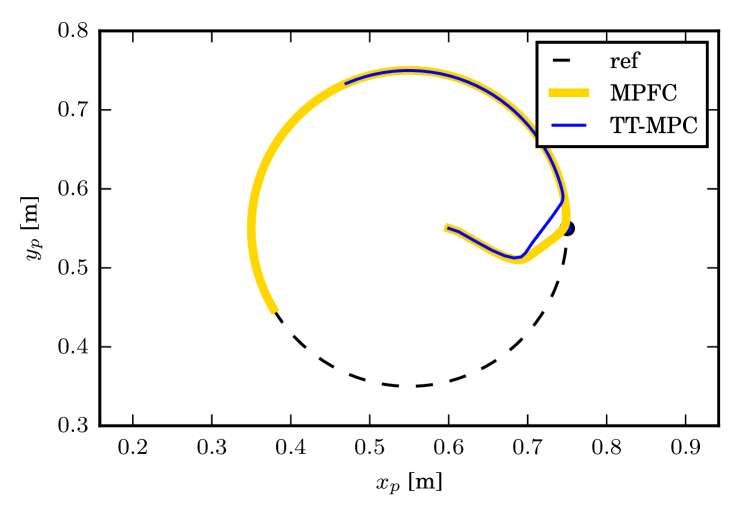
Figure 2: TT-MPC and MPFC moving from the same start point towards the path. The blue dot is the start of the reference path.

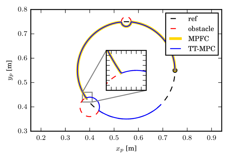
Figure 3: TT-MPC and MPFC initialized close to the path origin. The path is obstructed by a small and a large object. Both controllers pass the first object, but the MPFC does not pass the second.

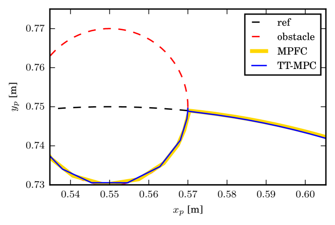
(a) Collocation method

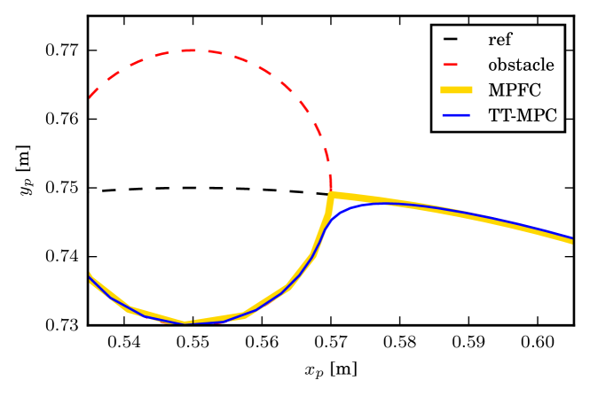
(b) RK4

Figure 4: Difference between the two integration methods when the path is obstructed. Only evident in TT-MPC as the MPFC slows sufficiently down before the obstacle to not encounter the integration problems.

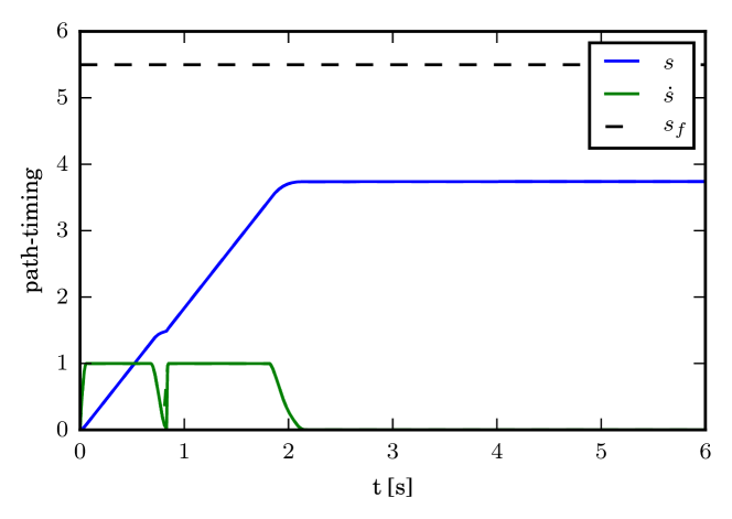
Figure 5: Timing parameter $s$, blue line, and $\dot{s}$, green line, when MPFC follows the obstructed path. First object encountered at $t\approx 0.9$s, second object encountered at $t\approx 2$s.

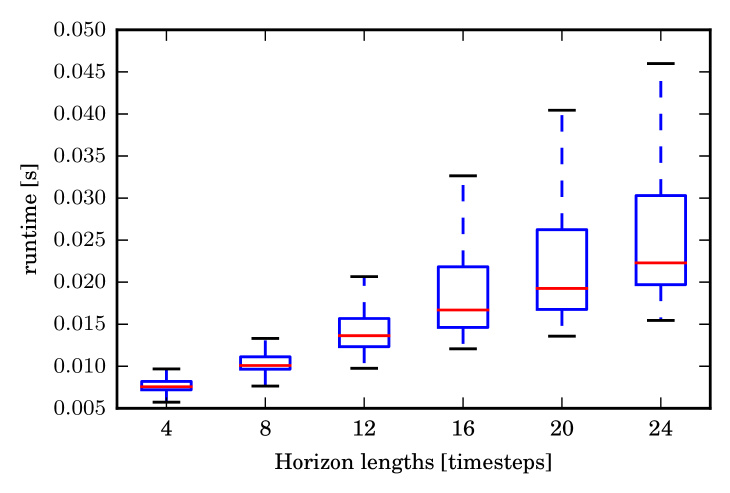
Figure 6: Boxplot of 2000 RK4 MPFC solver run times.

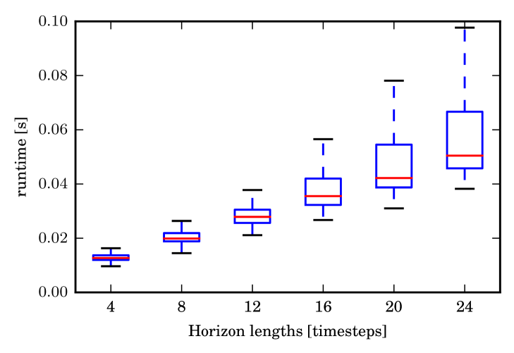
Figure 7: Boxplot of 2000 collocation MPFC solver run times.

TABLE III: Typical timing statistics T = 0.6

	Constr.	$\nabla_{\bm{q}}$Constr.	$\bm{H}(\mathcal{L})$	Iter.	Solver tot.
MPFC-RK4	0.03 ms	0.16 ms	0.52 ms	27	0.045 s
MPFC-Col	0.03 ms	0.08 ms	0.15 ms	24	0.102 s
TT-MPC-RK4	0.03 ms	0.23 ms	0.66 ms	14	0.039 s
TT-MPC-Col	0.03 ms	0.07 ms	0.11 ms	14	0.046 s

IV Discussion and Future work

The collocation method has a sparse structure in the equality constraints, and relies on evaluation of $\bm{f_{\xi}}$, whereas the RK4 requires evaluation of its algorithimic differentiation. This gives the collocation method faster function evaluations, but it did not appear to be sufficient to make the collocation method faster than RK4. The solver itself took more time with the increased number of states. For systems with complex dynamics the collocation method may be necessary. TT-MPC had fewer states, simpler dynamics and was faster on the whole, with the same observations as for the MPFC regarding integration method.

The MPFC has the ability to stop along its path. For time-critical systems this is not desired, but for robots in open environments it can prove useful. It also suggests that when obstructed by an unknown object, it may push against the object with a constant force. In future experiments this will be investigated further. The TT-MPC will observe a growing difference in the current position and the desired position. With a known obstruction it will project the path onto the constraint attempting to minimize the path error. Suddenly removing the obstruction should result in the TT-MPC moving towards its current set point as fast as possible. With an unknown obstruction the TT-MPC may exert a gradually increasing force on the obstruction.

For the MPC to be real-time feasible, we require the solver to run faster than the control interval used. In this article we have considered a control interval of length $\delta_{t}=0.01$ s. For low horizon lengths we are approaching such timing with the CasADi running in Python. Future work will extend this framework for a 6 degrees-of-freedom robot with a 3D path. The low horizon length needed to be able to achieve fast run time of the solver suggests that terminal constraints may be required in the final system.

The obstructions considered in this article were static and known apriori. Future work may include varying number of obstacles that enter the robot workspace.

V Conclusion

The model predictive path-following controller gives rise to a set of new design opportunities. Of most value for obstructed environments is the fact that it may freely stop and resume along its path. The question is whether a constraint ends the path, as the path-following controller did, or whether the robot should move along the path projected onto the constraint, as the trajectory tracking controller did.

We also saw that the interior point method of IPOPT interfaced through CasADi in Python, approached timings we would desire in a real-time systems.

VI Acknowledgements

The work reported in this paper was based on activities within centre for research based innovation SFI Manufacturing in Norway, and is partially funded by the Research Council of Norway under contract number 237900.

References

- [1] D. Verscheure, B. Demeulenaere, J. Swevers, J. De Schutter, and M. Diehl, “Time-optimal path tracking for robots: A convex optimization approach,” IEEE Transactions on Automatic Control, vol. 54, no. 10, pp. 2318–2327, 2009.
- [2] F. Debrouwere, W. Van Loock, G. Pipeleers, M. Diehl, J. Swevers, and J. De Schutter, “Convex time-optimal robot path following with Cartesian acceleration and inertial force and torque constraints,” Proceedings of the Institution of Mechanical Engineers, Part I: Journal of Systems and Control Engineering, vol. 227, no. 10, pp. 724–732, nov 2013.
- [3] T. Faulwasser, B. Kern, and R. Findeisen, “Model predictive path-following for constrained nonlinear systems,” Proceedings of the 48h IEEE Conference on Decision and Control (CDC) held jointly with 2009 28th Chinese Control Conference, no. 3, pp. 8642–8647, 2009.
- [4] T. Faulwasser and R. Findeisen, “Nonlinear Model Predictive Control for Constrained Output Path Following,” IEEE Transactions on Automatic Control, vol. 9286, no. c, pp. 1–1, 2016.
- [5] T. Faulwasser, T. Weber, P. Zometa, and R. Findeisen, “Implementation of Nonlinear Model Predictive Path-Following Control for an Industrial Robot,” IEEE Transactions on Control Systems Technology, pp. 1–7, 2016.
- [6] B. Houska, H. J. Ferreau, and M. Diehl, “ACADO Toolkit – An Open Source Framework for Automatic Control and Dynamic Optimization,” Optimal Control Applications and Methods, vol. 32, no. 3, pp. 298–312, 2011.
- [7] D. Lam, C. Manzie, and M. Good, “Model predictive contouring control,” in 49th IEEE Conference on Decision and Control (CDC), vol. 86, no. 8. IEEE, dec 2010, pp. 6137–6142.
- [8] ——, “Application of model predictive contouring control to an X-Y table,” IFAC Proceedings Volumes (IFAC-PapersOnline), vol. 18, no. PART 1, pp. 10 325–10 330, 2011.
- [9] M. Böck and A. Kugi, “Real-time nonlinear model predictive path-following control of a laboratory tower crane,” IEEE Transactions on Control Systems Technology, vol. 22, no. 4, pp. 1461–1473, 2014.
- [10] J. Andersson, “A General-Purpose Software Framework for Dynamic Optimization,” PhD thesis, Arenberg Doctoral School, KU Leuven, Belgium, 2013.
- [11] O. Egeland and J. T. Gravdahl, Modeling and Simulation for Automatic Control. Trondheim: Marine Cybernetics, 2003.
- [12] A. Wächter and L. T. Biegler, On the Implementation of Primal-Dual Interior Point Filter Line Search Algorithm for Large-Scale Nonlinear Programming, 2006, vol. 106, no. 1.
- [13] A. Astolfi, D. Karagiannis, and R. Ortega, Nonlinear and Adaptive Control with Applications (Communications and Control Engineering), 2007.