Scalable Collaborative Targeted Learning for High-Dimensional Data

Abstract

Robust inference of a low-dimensional parameter in a large semi-parametric model relies on external estimators of infinite-dimensional features of the distribution of the data. Typically, only one of the latter is optimized for the sake of constructing a well behaved estimator of the low-dimensional parameter of interest. Optimizing more than one of them for the sake of achieving a better bias-variance trade-off in the estimation of the parameter of interest is the core idea driving the general template of the collaborative targeted minimum loss-based estimation (C-TMLE) procedure.

The original implementation/instantiation of the C-TMLE template can be presented as a greedy forward stepwise C-TMLE algorithm. It does not scale well when the number $p$ of covariates increases drastically. This motivates the introduction of a novel implementation/instantiation of the C-TMLE template where the covariates are pre-ordered. Its time complexity is $\mathcal{O}(p)$ as opposed to the original $\mathcal{O}(p^{2})$, a remarkable gain. We propose two pre-ordering strategies and suggest a rule of thumb to develop other meaningful strategies. Because it is usually unclear a priori which pre-ordering strategy to choose, we also introduce another implementation/instantiation called SL-C-TMLE algorithm that enables the data-driven choice of the better pre-ordering strategy given the problem at hand. Its time complexity is $\mathcal{O}(p)$ as well.

The computational burden and relative performance of these algorithms were compared in simulation studies involving fully synthetic data or partially synthetic data based on a real world large electronic health database; and in analyses of three real, large electronic health databases. In all analyses involving electronic health databases, the greedy C-TMLE algorithm is unacceptably slow. Simulation studies indicate our scalable C-TMLE and SL-C-TMLE algorithms work well. All C-TMLEs are publicly available in a Julia software package.

1 Introduction

The general template of collaborative double robust targeted minimum loss-based estimation (C-TMLE; “C-TMLE template” for short) builds upon the targeted minimum loss-based estimation (TMLE) template (van der Laan and Rose, 2011, van der Laan and Gruber, 2010). Both the TMLE and C-TMLE templates can be viewed as meta-algorithms which map a set of user-supplied choices/hyper-parameters ( e.g., parameter of interest, loss function, submodels) into a specific machine-learning algorithm for estimation, that we call an instantiation of the template.

Constructing a TMLE or a C-TMLE involves the estimation of a nuisance parameter, typically an infinite-dimensional feature of the distribution of the data. For a vanilla TMLE estimator, the estimation of the nuisance parameter is addressed as an independent statistical task. In the C-TMLE template, on the contrary, the estimation of the nuisance parameter is optimized to provide a better bias-variance trade-off in the inference of the targeted parameter. The C-TMLE template has been successfully applied in a variety of areas, from survival analysis (Stitelman et al., 2011), to the study of gene association (Wang et al., 2011) and longitudinal data structures (Stitelman and van der Laan, 2010) to name just a few.

In the original instantiation of the C-TMLE template of van der Laan and Gruber (2010), that we henceforth call “the greedy C-TMLE algorithm”, the estimation of the nuisance parameter aiming for a better bias-variance trade-off is conducted in two steps. First, a greedy forward stepwise selection procedure is implemented to construct a nested sequence of candidate estimators of the nuisance parameter. Second, cross-validation is used to select the candidate from this sequence which minimizes a criterion that incorporates a measure of bias and variance with respect to (wrt) the targeted parameter (the algorithm is described in Section 4). The authors show the greedy C-TMLE algorithm exhibits superior relative performance in analyses of sparse data, at the cost of an increase in time complexity. For instance, in a problem with $p$ baseline covariates, one would construct and select from $p$ candidate estimators of the nuisance parameter, yielding a time complexity of order $\mathcal{O}(p^{2})$. Despite a criterion for early termination, the algorithm does not scale to large-scale and high-dimensional data. The aim of this article is to develop novel C-TMLE algorithms that overcome these serious practical limitations without compromising finite sample or asymptotic performance.

We propose two such “scalable C-TMLE algorithms”. They replace the greedy search at each step by an easily computed data adaptive pre-ordering of the candidate estimators of the nuisance parameter. They include a data adaptive, early stopping rule that further reduces computational time without sacrificing statistical performance. In the aforementioned problem with $p$ baseline covariates where the time complexity of the greedy C-TMLE algorithm was of order $\mathcal{O}(p^{2})$, those of the two novel scalable C-TMLE algorithms is of order $\mathcal{O}(p)$.

Because one may be reluctant to specify a single a priori pre-ordering of the candidate estimators of the nuisance parameter, we also introduce a SL-C-TMLE algorithm. It selects the best pre-ordering from a set of ordering strategies by super learning (SL) (van der Laan et al., 2007). SL is an example of ensemble learning methodology which builds a meta-algorithm for estimation out of a collection of individual, competing algorithms of estimation, relying on oracle properties of cross-validation.

We focus on the estimation of the average (causal) treatment effect (ATE). It is not hard to generalize our scalable C-TMLE algorithms to other estimation problems.

The performance of the two scalable C-TMLE and SL-C-TMLE algorithms are compared with those of competing, well established estimation methods: G-computation (Robins, 1986), inverse probability of treatment weighting (IPTW) (Hernan et al., 2000, Robins, 2000b), augmented inverse probability of treatment weighted estimator (A-IPTW) (Robins and Rotnitzky, 2001, Robins et al., 2000b, Robins, 2000a). Results from unadjusted regression estimation of a point treatment effect are also provided to illustrate the level of bias due to confounding.

The article is organized as follows. Section 2 introduces the parameter of interest and a causal model for its causal interpretation. Section 3 describes an instantiation of the TMLE template. Section 4 presents the C-TMLE template and a greedy instantiation of it. Section 5 introduces the two proposed pre-ordered scalable C-TMLE algorithms, and SL-C-TMLE algorithm. Sections 6 and 7 present the results of simulation studies (based on fully or partially synthetic data, respectively) comparing the C-TMLE and SL-C-TMLE estimators with other common estimators. Section 8 is a closing discussion. The appendix presents additional material: an introduction to a Julia software that implements all the proposed C-TMLE algorithms; a brief analysis of their computational performance; the results of their application to the analysis of three large electronic health databases.

2 The Average Treatment Effect Example

We consider the problem of estimating the ATE in an observational study where we observe on each experimental unit: a collection of $p$ baseline covariates, $W$; a binary treatment indicator, $A$; a binary or bounded continuous $(0,1)$-valued outcome of interest, $Y$. We use $O_{i}=(W_{i},A_{i},Y_{i})$ to represent the $i$-th observation from the unknown observed data distribution $P_{0}$, and assume that $O_{1},\ldots,O_{n}$ are independent. The parameter of interest is defined as

$$\Psi(P_{0})=\operatorname{\mathbb{E}}_{0}[\operatorname{\mathbb{E}}_{0}(Y\mid A=1,W)-\operatorname{\mathbb{E}}_{0}(Y\mid A=0,W)].$$

The ATE enjoys a causal interpretation under the non-parametric structural equation model (NPSEM) given by:

$$\left\{\begin{array}[]{l}W=f_{W}(U_{W}),\\ A=f_{A}(W,U_{A}),\\ Y=f_{Y}(A,W,U_{Y}),\end{array},\right.$$

where $f_{W}$, $f_{A}$ and $f_{Y}$ are deterministic functions and $U_{W},U_{A},U_{Y}$ are background (exogenous) variables. The potential outcome under exposure level $a\in\{0,1\}$ can be obtained by substituting $a$ for $A$ in the third equality: $Y_{a}=f_{Y}(a,W,U_{Y})$. Note that $Y=Y_{A}$ (this is known as the “consistency” assumption). If we are willing to assume that (i) $A$ is conditionally independent of $(Y_{1},Y_{0})$ given $W$ (this is known as the “no unmeasured confounders” assumption) and (ii) $0<P(A=1\mid W)<1$ almost everywhere (known as the “positivity” assumption), then parameter $\Psi(P_{0})$ satisfies $\Psi(P_{0})=\operatorname{\mathbb{E}}_{0}(Y_{1}-Y_{0})$.

For future use, we introduce the propensity score (PS), defined as the conditional probability of receiving treatment, and define $g_{0}(a,W)\equiv P_{0}(A=a\mid W)$ for both $a=0,1$. We also introduce the conditional mean of the outcome: $\bar{Q}_{0}(A,W)=\operatorname{\mathbb{E}}_{0}(Y\mid A,W)$. In the remainder of this article, $g_{n}(a,W)$ and $\bar{Q}_{n}(A,W)$ denote estimators of $g_{0}(a,W)$ and $\bar{Q}_{0}(A,W)$.

3 A TMLE Instantiation for ATE

We are mainly interested in double robust (DR) estimators of $\Psi(P_{0})$. An estimator of $\Psi(P_{0})$ is said to be DR if it is consistent if either $\bar{Q}_{0}$ or $g_{0}$ is consistently estimated. In addition, an estimator of $\Psi(P_{0})$ is said to be efficient if it satisfies a central limit theorem with a limit variance which equals the second moment under $P_{0}$ of the so called efficient influence curve (EIC) at $P_{0}$. The EIC for the ATE parameter is given by

$$D^{*}(\bar{Q}_{0},g_{0})(O)=H_{0}(A,W)[Y-\bar{Q}_{0}(A,W)]+\bar{Q}_{0}(1,W)-\bar{Q}_{0}(0,W)-\Psi(P_{0}),$$

where $H_{0}(a,W)=a/g_{0}(1,W)-(1-a)/g_{0}(0,W)$ ($a=0,1)$. The notation is slightly misleading because there is more to $\Psi(P_{0})$ than $(\bar{Q}_{0},g_{0})$ (namely, the marginal distribution of $W$ under $P_{0}$). We nevertheless keep it that way for brevity. We refer the reader to (Bickel et al., 1998) for details about efficient influence curves.

More generally, for every valid distribution $P$ of $O=(W,A,Y)$ such that (i) the conditional expectation of $Y$ given $(A,W)$ equals $\bar{Q}(A,W)$ and the conditional probability that $A=a$ given $W$ equals $g(a,W)$, and (ii) $0<g(1,W)<1$ almost surely, we denote

$$D^{*}(\bar{Q},g)(O)=H_{g}(A,W)[Y-\bar{Q}(A,W)]+\bar{Q}(1,W)-\bar{Q}(0,W)-\Psi(P),$$

where $H_{g}(a,W)=a/g(1,W)-(1-a)/g(0,W)$ ($a=0,1$).

The augmented inverse probability of treatment weighted estimator (A-IPTW, or so called “double robust IPTW”; Robins et al. (1994, 2000a), van der Laan and Dudoit (2003)) and TMLE (van der Laan and Rubin, 2006, van der Laan and Rose, 2011) are two well studied DR estimators. Taking the estimation of ATE as an example, A-IPTW estimates $\Psi(P_{0})$ by solving the EIC equation directly. For given estimators $\bar{Q}_{n}$, $g_{n}$ and with

$$H_{g_{n}}(a,W)=a/g_{n}(1,W)-(1-a)/g_{n}(0,W)\quad(a=0,1),$$ (1)

solving (in $\psi$)

$$0 = \sum_{i=1}^{n}H_{g_{n}}(A_{i},W_{i})[Y_{i}-\bar{Q}_{n}(A_{i},W_{i})]+\bar{Q}_{n}(1,W_{i})-\bar{Q}_{n}(0,W_{i})-\psi$$

yields the A-IPTW estimator

$$\psi_{n}^{A-IPTW}=\sum_{i=1}^{n}H_{g_{n}}(A_{i},W_{i})[Y_{i}-\bar{Q}_{n}(A_{i},W_{i})]+\bar{Q}_{n}(1,W_{i})-\bar{Q}_{n}(0,W_{i}).$$

A substitution (or plug-in) estimator of $\Psi(P_{0})$ is obtained by plugging-in the estimator of a relevant part of the data-generating distribution $P_{0}$ into the mapping $\Psi$. Substitution estimators belong to the parameter space by definition, which is a desirable property. The A-IPTW is not a substitution estimator and can suffer from it by sometimes producing estimates outside of known bounds on the problem, such as probabilities or proportions greater than 1. On the contrary, an instantiation of the TMLE template yields a DR TMLE estimator defined by substitution. For instance, a TMLE estimator can be can be constructed by applying the TMLE algorithm below (which corresponds to the negative $\log$-likelihood loss function and logistic fluctuation submodels).

1. Estimating $\bar{Q}_{0}$. Derive an initial estimator $\bar{Q}_{n}^{0}$ of $\bar{Q}_{0}$. It is highly recommended to avoid making parametric assumptions, as any parametric model is likely mis-specified. Relying on SL (van der Laan et al., 2007) is a good option.

2. Estimating $g_{0}$. Derive an estimator $g_{n}$ of $g_{0}$, The same recommendation as above applies.

3. Building the so called “clever covariates”. For $a=0,1$ and a generic $W$, define $H_{n}(a,W)$ as in (1).

4. Targeting. Fit the logistic regression of $Y_{i}$ on $H_{n}(A_{i},W_{i})$ with no intercept, using $\operatorname*{logit}(\bar{Q}_{n}^{0}(A_{i},W_{i}))$ as offset (an $i$-specific intercept). This yields a minimum loss estimator $\epsilon_{n}$. Update the initial estimator $\bar{Q}_{n}^{0}$ into $\bar{Q}_{n}^{*}$ given by

   $$\bar{Q}_{n}^{*}(A,W)=\operatorname*{expit}\{\operatorname*{logit}[\bar{Q}_{n}^{0}(A,W)]+\epsilon_{n}H_{n}(A,W)\}.$$

5. Evaluating the parameter estimate. Define

   $$\psi_{n}^{TMLE}=\frac{1}{n}\sum_{i=1}^{n}(\bar{Q}_{n}^{*}(1,W_{i})-\bar{Q}_{n}^{*}(0,W_{i})).$$ (2)

   As emphasized, TMLE is a substitution estimator.

The targeting step aims to reduce bias in the estimation of $\Psi(P_{0})$ by enhancing the initial estimator derived from $\bar{Q}_{n}^{0}$ and the marginal empirical distribution of $W$ as an estimator of its counterpart under $P_{0}$. The fluctuation is made in such a way that the EIC equation is solved: $\sum D^{*}(\bar{Q}^{*}_{n},g_{n})(O_{i})=0$. Therefore, the TMLE estimator is double robust and (locally) efficient under regularity conditions (van der Laan and Rose, 2011).

Standard errors and confidence intervals (CIs) can be computed based on the variance of the influence curve. Proofs and technical details are available in the literature (van der Laan and Rubin, 2006, van der Laan and Rose, 2011, for instance).

In practice, bounded continuous outcomes and binary outcomes are fluctuated on the $\operatorname*{logit}$ scale to ensure that bounds on the model space are respected (Gruber and van der Laan, 2010b).

4 The C-TMLE General Template and Its Greedy Instantiation for ATE

When implementing an instantiation of the TMLE template, one relies on a single external estimate of the nuisance parameter, $g_{0}$ in the ATE example (see Step 2 in Section 3). In contrast, an instantiation of the C-TMLE template involves constructing a series of nuisance parameter estimates and corresponding TMLE estimators using these estimates in the targeting step.

4.1 The C-TMLE Template

When the ATE is the parameter of interest, the C-TMLE template can be summarized recursively like this (see Algorithm 1 for a high-level algorithmic presentation). One first builds $(g_{n,0},\bar{Q}_{n}^{0}=\bar{Q}_{n,0},\bar{Q}_{n,0}^{*})$ where $g_{n,0}$ is an estimator of $g_{0}$ and $\bar{Q}_{n}^{0}=\bar{Q}_{n,0},\bar{Q}_{n,0}^{*}$ are estimators of $\bar{Q}_{0}$, the latter being targeted toward the parameter of interest for instance as in Section 3. Given the previous triplets $(g_{n,0},\bar{Q}_{n}^{0}=\bar{Q}_{n,0},\bar{Q}_{n,0}^{*}),\ldots,(g_{n,k-1},\bar{Q}_{n,k-1},\bar{Q}_{n,k-1}^{*})$ where, by construction, the empirical loss of each $\bar{Q}_{n,\ell}^{*}$ is smaller than that of $\bar{Q}_{n,\ell-1}^{*}$, one needs to generate the next triplet in the sequence. The current initial estimator of $\bar{Q}_{0}$ at the $(k+1)$-th step is set at $\bar{Q}_{n,k}=\bar{Q}_{n,k-1}$ (i.e., the same as that from triplet $(g_{n,k-1},\bar{Q}_{n,k-1},\bar{Q}_{n,k-1}^{*})$). One then has a set of moves to create candidates $g_{n,k}^{j}$ updating $g_{n,k-1}$ with move $j$ (e.g., adding $j$-th covariate), providing better empirical fit than $g_{n,k-1}$ and yielding the corresponding $\bar{Q}_{n,k}^{j,*}$ using $\bar{Q}_{n,k}=\bar{Q}_{n,k-1}$ as initial. The candidate with the smallest empirical loss is $(g_{n,k},\bar{Q}_{n,k},\bar{Q}_{n,k}^{*})$. Two cases arise: if the empirical loss of the candidate $\bar{Q}_{n,k}^{*}$ is smaller than that of $\bar{Q}_{n,k-1}^{*}$, then one has derived the next triplet $(g_{n,k},\bar{Q}_{n,k}=\bar{Q}_{n,k-1},\bar{Q}_{n,k}^{*})$; otherwise, in our sequence, one updates the initial $\bar{Q}_{n,k}=\bar{Q}_{n,k-1}^{*}$ to the $\bar{Q}_{n,k-1}^{*}$ in the last triplet, and one repeats the above to generate $(g_{n,k},\bar{Q}_{n,k},\bar{Q}_{n,k}^{*})$ – since it is now guaranteed that the empirical loss of $\bar{Q}_{n,k}^{*}$ is smaller that that of $\bar{Q}_{n,k-1}^{*}$, one always gets the desired next element $(g_{n,k},\bar{Q}_{n,k},\bar{Q}_{n,k}^{*})$.

In the original greedy C-TMLE algorithm (van der Laan and Gruber, 2010), the successive nuisance parameter estimates are based on a data-adaptive forward stepwise search that optimizes a goodness-of-fit criterion at each step. Each of them then yields a specific, candidate TMLE. Finally, the C-TMLE is defined as that candidate that optimizes a cross-validated version of the criterion. The C-TMLE inherits all the properties of a vanilla TMLE estimator (van der Laan and Gruber, 2010). It is double robust and asymptotically efficient under appropriate regularity conditions.

Algorithm 1 General Template of C-TMLE

1:Construct an initial estimate $\bar{Q}_{n}^{0}$ for $\bar{Q}_{0}.$

2:Create candidate $\bar{Q}_{n,k}^{*}$, using different estimates of treatment mechanism $g_{0}$, such that the empirical losses of $\bar{Q}_{n,k}^{*}$ and $g_{n,k}$ are decreasing in $k$. The greedy C-TMLE algorithm uses a forward greedy selection algorithm.

3:Select the best candidate $\bar{Q}_{n}^{*}=\bar{Q}_{n,k_{n}}^{*}$ using loss-based cross-validation, with the same loss function as in the TMLE targeting step.

In Step 1 of Algorithm 1, we recommend using SL as described further in Section 3. Step 2 will be commented on in the next section. In Step 3, the best candidate is selected based on the cross-validated penalized log-likelihood and indexed by

$$k_{n}=\operatorname*{arg\,min}_{k}\left\{{\rm cvRSS}+{\rm cvVar}_{k}+n\times{\rm cvBias}_{k}^{2}\right\}$$

where

$${\rm cvRSS}_{k} = \sum_{v=1}^{V}\sum_{i\in{\rm Val}(v)}(Y_{i}-\bar{Q}_{n,k}^{*}(P^{0}_{nv})(W_{i},A_{i}))^{2},$$

$${\rm cvVar}_{k} = \sum_{v=1}^{V}\sum_{i\in{\rm Val}(v)}D^{*2}(\bar{Q}_{n,k}^{*}(P^{0}_{nv}),g_{n,k}(P_{n}))(O_{i}),$$

$${\rm cvBias}_{k} = \frac{1}{V}\sum_{v=1}^{V}\Psi(\bar{Q}_{n,k}^{*}(P_{nv}^{0}))-\Psi(\bar{Q}_{n,k}^{*}(P_{n})).$$

In the above display, ${\rm Val}(v)$ is the set of indices of observations used for validation in the $v$-th fold, $P_{nv}^{0}$ is the empirical distribution of the observations indexed by $i\not\in{\rm Val}(v)$, $P_{n}$ is the empirical distribution of the whole data set, and $Z(P_{nv}^{0})$ (respectively, $Z(P_{n})$) means that $Z$ is fitted using $P_{nv}^{0}$ (respectively, $P_{n}$). The penalization terms ${\rm cvVar}_{k}$ and ${\rm cvBias}_{k}$ robustify the finite sample performance when the positivity assumption is violated (van der Laan and Gruber, 2010).

To achieve collaborative double robustness, the sequence of estimators $(g_{n,k}:k)$ should be arranged in such a way that the bias is monotonically decreasing while the variance is monotonically increasing such that $g_{n,k}$ converges (in $k$) to a consistent estimator of $g_{0}$ (van der Laan and Rose, 2011). One could for instance rely on a nested sequence of models, see Section 4.2. By doing so, the empirical fit for $g_{0}$ improves as $k$ increases (van der Laan and Rose, 2011, Gruber and van der Laan, 2010a).

Porter et al. (2011) discuss and compare TMLE and C-TMLE with other DR estimators, including A-IPTW.

4.2 The Greedy C-TMLE Algorithm

We refer to the original instantiation of the C-TMLE template as the greedy C-TMLE algorithm. It uses a forward selection algorithm to build the sequence of estimators of $g_{0}$ as a nested sequence of treatment models. Let us describe it in the case that $W$ consists of $p$ covariates. For $k=0$, a one-dimensional logistic model with only an intercept is used to estimate $g_{0}$. Recursively, the $(k+1)$th model is derived by adding one more covariate from $W$ to the $k$th logistic model. The chosen covariate is selected from the set of covariates in $W$ that have not been selected so far.

More specifically, one begins with the intercept model for $g_{0}$ to construct $g_{n,0}$ then a first fluctuation covariate $H_{g_{n,0}}$ as in (1), which is used in turn to create the first candidate estimator $\bar{Q}_{n,0}^{*}$ based on $\bar{Q}_{n,0}$. Namely, denoting $g_{n,0}(1\mid W)=P_{n}(A=1)$ and $g_{n,0}(0\mid W)=P_{n}(A=0)$, we set

$$H_{g_{n,k}}(a,W) = a/g_{n,k}(1\mid W)-(1-a)/g_{n,k}(0\mid W),$$ (3)

$$\operatorname*{logit}(\bar{Q}_{n,k}^{*}(a,W)) = \operatorname*{logit}(\bar{Q}_{n,k}(a,W))+\epsilon_{k}H_{g_{n,k}}(a,W)\quad(a=0,1)$$ (4)

where $k=0$. Here $\epsilon_{k}$ is fitted by a logistic regression of $Y$ on $H_{g_{n,k}}(A,W)$ with offset $\bar{Q}_{n,k}(A,W)$, and $\bar{Q}_{n,1}^{*}$ is the first candidate TMLE. We denote ${\cal L}_{0}$ its empirical loss wrt the negative $\log$-likelihood function ${\cal L}$.

We proceed recursively. Assume that we have already derived $\bar{Q}_{n,0}^{*},\ldots$, $\bar{Q}_{n,k-1}^{*}$, and denote the initial estimator used in the last TMLE $\bar{Q}_{n,k-1}^{*}$ with $\bar{Q}_{n,k-1}$. The $(k+1)$-th estimator $g_{n,k}$ of $g_{0}$ is based on a larger model than that we yielded $g_{n,k-1}$. It contains the intercept and the same $(k-1)$ covariates as the previous model fit $g_{n,k-1}$, with one additional covariate. Each covariate $W_{j}$ ($1\leq j\leq p$ such that $W_{j}$ has not been selected yet) is considered in turn for inclusion in the model, yielding a update $g_{n,k}^{j}$ of $g_{n,k-1}$, which implies corresponding updates $H_{g_{n,k}}^{j}$ and $\bar{Q}_{n,k}^{j,*}$ as in the above display. A best update $\bar{Q}_{n,k}^{*}$ is selected among the candidate updates $\bar{Q}_{n,k}^{1,*},\ldots,\bar{Q}_{n,k}^{p,*}$ by minimizing the empirical loss wrt ${\cal L}$. Its empirical loss is denoted ${\cal L}_{k}$. If ${\cal L}_{k}\leq{\cal L}_{k-1}$, then this $\bar{Q}_{n,k}^{*}$ defines the next fluctuation in our sequence, with corresponding initial estimator still $\bar{Q}_{n,k}=\bar{Q}_{n,k-1}$, the same as that used to build $\bar{Q}_{n,k-1}^{*}$. We can now move on to the next step. Otherwise, we reset the initial estimator $\bar{Q}_{n,k-1}$ to $\bar{Q}_{n,k-1}^{*}$ and repeat the above procedure: i.e., we compute the candidate updates $\bar{Q}_{n,k}^{j,*}$ again for this new initial estimator, and select the best choice $\bar{Q}_{n,k}^{*}$. Due to the initial estimator in $\bar{Q}_{n,k}^{*}$ being $\bar{Q}_{n,k-1}^{*}$, it is now guaranteed that the new ${\cal L}_{k}$ is smaller than ${\cal L}_{k-1}$, thereby providing us with our next TMLE $\bar{Q}_{n,k}^{*}$ in our sequence.

This forward stepwise procedure is carried out recursively until all $p$ covariates have been incorporated into the model for $g_{0}$. In the discussed setting, choosing the first covariate requires $p$ comparisons, choosing the second covariate requires $(p-1)$ comparisons and so on, making the time complexity of this algorithm $\mathcal{O}(p^{2})$.

Once all candidates $\bar{Q}_{n,0}^{*},\ldots,\bar{Q}_{n,k}^{*}$ have been constructed, cross-validation is used to select the optimal number of covariates to include in the model for $g_{0}$. For more concrete examples, we refer to (van der Laan and Gruber, 2010, van der Laan and Rose, 2011). Gruber and van der Laan (2010a) proposes several variations on the forward greedy stepwise C-TMLE algorithm. The variations did not improve performance in simulation studies. In this article, the greedy C-TMLE algorithm is defined by the procedure described above.

5 Scalable C-TMLE Algorithms

Now that we have introduced the background on C-TMLE, we will now introduce our scalable C-TMLE algorithm. Section 5.1 summarizes the philosophy of the scalable C-TMLE algorithm, which hinges on a data adaptively determined pre-ordering of the baseline covariates. Sections 5.2 and 5.3 present two such pre-ordering strategies. Section 5.4 discusses what properties a pre-ordering strategy should satisfy. Finally, Section 5.5 proposes a discrete Super Learner-based model selection procedure to select among a set of scalable C-TMLE estimators, which is itself a scalable C-TMLE algorithm.

5.1 Outline

As we have seen in the previous section, the time complexity of the greedy C-TMLE algorithm is $\mathcal{O}(p^{2})$ when the number of covariates equals $p$. This is unsatisfactory for large scale and high-dimensional data, which is an increasingly common situation in health care research. For example, the high-dimensional propensity score (hdPS) algorithm is a method to extract information from electronic medical claims data that produces hundreds or even thousands of candidate covariates, increasing the dimension of the data dramatically (Schneeweiss et al., 2009).

In order to make it possible to apply C-TMLE algorithms to such data sets, we propose to add a new pre-ordering procedure after the initial estimation of $\bar{Q}_{0}$ and before the stepwise construction of the candidate $\bar{Q}_{n,k}^{*}$, $k=0,\ldots$. We present two pre-ordering procedures in Sections 5.2 and 5.3. By imposing an ordering over the covariates only one covariate is eligible for inclusion in the PS model at each step when constructing the next candidate TMLE in the sequence, $\bar{Q}_{n,k}^{*}$. Thus, the new C-TMLE algorithm overcomes the computational issue.

Once an ordering over the covariates has been established, we add them one by one to the model used to estimate $g_{0}$, starting from the intercept model. Suppose that we are adding the $k$th covariate; we obtain a new estimate $g_{n,k}$ of $g_{0}$; we define a new clever covariate as in (3); we fluctuate the current initial estimator $\bar{Q}_{n}^{k}$ as in (4); we evaluate the empirical loss ${\cal L}_{k}$ wrt ${\cal L}$ of the resulting candidate $\bar{Q}_{n,k}^{*}$. If ${\cal L}_{k}\leq{\cal L}_{k-1}$, then we move on to adding the next covariate; otherwise, the current initial estimate $\bar{Q}_{n,k}$ is replaced by $\bar{Q}_{n,k-1}^{*}$ and we restart over adding the $k$th covariate. This approach guarantees that ${\cal L}_{k}\leq{\cal L}_{k-1}$.

Finally, we use cross-validation to select the best candidate among $\bar{Q}_{n,0}^{*},\ldots$, $\bar{Q}_{n,p}^{*}$ in terms of cross-validated loss wrt ${\cal L}$.

5.2 Logistic Pre-Ordering Strategy

The logistic pre-ordering procedure is similar to the second round of the greedy C-TMLE algorithm. However, instead of selecting one single covariate before going on, we use the empirical losses wrt ${\cal L}$ to order the covariates by their ability to reduce bias. More specifically, for each covariate $W_{k}$ ($1\leq k\leq p$), we construct an estimator $g_{n,k}$ of the conditional distribution of $A$ given $W_{k}$ only (one might also add $W_{k}$ to a fixed baseline model); we define a clever covariate as in (3) using $g_{n,k}$ and fluctuate $\bar{Q}_{n}^{0}$ as in (4); we compute the empirical loss of the resulting $\bar{Q}_{n,k}^{*}$ wrt ${\cal L}$, yielding ${\cal L}_{k}$. Finally, the covariates are ranked by increasing values of the empirical loss. This is summarized in Algorithm 2.

Algorithm 2 Logistic Pre-Ordering Algorithm

1:for each covariate $W_{k}$ in $W$ do

2:     Construct an estimator $g_{n,k}$ of $g_{0}$ using a logistic model with $W_{k}$ as predictor.

3:     Define a clever covariate $H_{g_{n,k}}(A,W_{k})$ as in (3).

4:     Fit $\epsilon_{k}$ by regressing $Y$ on $H_{g_{n,k}}(A,W_{k})$ with offset $\bar{Q}_{n}^{0}(A,W)$.

5:     Define $\bar{Q}_{n,k}^{*}$ as in (4).

6:     Compute the empirical loss ${\cal L}_{k}$ wrt ${\cal L}$.

7:end for

8:Rank the covariates by increasing ${\cal L}_{k}$.

5.3 Partial Correlation Pre-Ordering Strategy

In the greedy C-TMLE algorithm described in Section 4.2, once $k$ covariates have already been selected, the $(k+1)$th is that remaining covariate which provides the largest reduction in the empirical loss wrt ${\cal L}$. Intuitively, the $(k+1)$th covariate is the one that best explains the residual between $Y$ and the current $\bar{Q}_{n}^{0}$. Drawing on this idea, the partial correlation pre-ordering procedure ranks the $p$ covariates based on how each of them is correlated with the residual between $Y$ and the initial $\bar{Q}_{n}^{0}$ within strata of $A$. This second strategy is less computationally demanding than the previous one because there is no need to fit any regression models, merely to estimate $p$ partial correlation coefficients.

Let $\rho(X_{1},X_{2})$ denote the Pearson correlation coefficient between $X_{1}$ and $X_{2}$. Recall that the partial correlation $\rho(X_{1},X_{2}|X_{3})$ between $X_{1}$ and $X_{2}$ given $X_{3}$ is defined as the correlation coefficient between the residuals $R_{X_{1}}$ and $R_{X_{2}}$ resulting from the linear regression of $X_{1}$ on $X_{3}$ and of $X_{2}$ on $X_{3}$, respectively (Hair et al., 2006). For each $1\leq k\leq p$, we introduce $R=Y-\bar{Q}_{n}^{0}(A,W)$,

$$\rho(R,W_{k}|A)=\frac{\rho(R,W_{k})-\rho(R,A)\times\rho(W_{k},A)}{\sqrt{(1-\rho(R,A)^{2})(1-\rho(W_{k},A)^{2})}}.$$

The partial correlation pre-ordering strategy is summarized in Algorithm 3.

Algorithm 3 Partial Correlation Pre-Ordering Algorithm

1:for each covariate $W_{k}$ in $W$ do

2:     Estimate the partial correlation coefficient $\rho(R,W_{k}|A)$ between $R=(Y-\bar{Q}_{n}^{0}(A,W))$ and $W_{k}$ given $A$.

3:end for

4:Rank the covariates based on the absolute value of the estimates of the partial correlation coefficients.

5.4 Discussion of the Design of Pre-ordering

Sections 5.2 and 5.3 proposed two pre-ordering strategies. In general, a rule of thumb for designing a pre-ordering strategy is to rank the covariates based on the impact of each in reducing the residual bias in the target parameter which results from the initial estimator $\bar{Q}_{n}^{0}$ of $\bar{Q}_{0}$. In this light, the logistic ordering of Section 5.2 uses TMLE to reflect the importance of each variable wrt its potential to reduce residual bias. The partial correlation ordering of Section 5.3 ranks the covariates according to the partial correlation of residual of the initial fit and the covariates, conditional on treatment.

Because the rule of thumb considers each covariate in turn separately, it is particularly relevant when the covariates are not too dependent. For example, consider the extreme case where two or more of the covariates are highly correlated and can greatly explain the residual bias in the target parameter. In this scenario, these dependent covariates would all be ranked towards the front of the ordering. However, after adjusting for one of them, the others would typically be much less helpful for reducing the remaining bias. This redundancy may harm the estimation. In cases where it is computationally feasible, this problem can be avoided by using the greedy search strategy, but many other intermediate strategies can be pursued as well.

5.5 Super Learner-Based C-TMLE Algorithm

Here, we explain how to combine several C-TMLE algorithms into one. The combination is based on a Super Learner (SL). Super learning is an ensemble machine learning approach that relies on cross-validation. It has been proven that a SL selector can perform asymptotically as well as an oracle selector under mild assumptions (van der Laan et al., 2007, van der Laan and Dudoit, 2003, van der Vaart et al., 2006).

As hinted at above, a SL-C-TMLE algorithm is an instantiation of an extension of the C-TMLE template. It builds upon several competing C-TMLE algorithms, each relying on different strategies to construct a sequence of estimators of the nuisance parameter. A SL-C-TMLE algorithm can be designed to select the single best strategy (discrete SL-C-TMLE algorithm), or an optimal combination thereof (ensemble SL-C-TMLE algorithm). A SL-C-TMLE algorithm can include both greedy search and pre-ordering methods. A SL-C-TMLE algorithm is scalable if all of the candidate C-TMLE algorithms in the library are scalable themselves.

We focus on a scalable discrete SL-C-TMLE algorithm that uses cross-validation to choose among candidate scalable (pre-ordered) C-TMLE algorithms. Algorithm 4 describes its steps. Note that a single cross-validation procedure is used to select both the ordering procedure $m$ and the number of covariates $k$ included in the PS model. It is because computational time is an issue that we do not rely on a nested cross-validation procedure to select $k$ for each pre-ordering strategy $m$.

Algorithm 4 Super Learner C-TMLE Algorithm

1:Define $M$ covariates pre-ordering strategies yielding $M$ C-TMLE algorithms

2:for each pre-ordering strategy $m$ do

3:     Follow step 2 of Algorithm 1 to create candidate $\bar{Q}_{n,m,k}^{*}$ for the $m$-th strategy.

4:end for

5:The best candidate $\bar{Q}_{n}^{*}$ is the minimizer of the cross-validated losses of $\bar{Q}_{n,m,k}^{*}$ across all the $(m,k)$ combinations.

The time complexity of the SL-C-TMLE algorithm is of the same order as that of the most complex C-TMLE algorithm considered. So, if only pre-ordering strategies of order $\mathcal{O}(p)$ are considered, then the time complexity of the SL-C-TMLE algorithm is $\mathcal{O}(p)$ as well. Given a constant number of user-supplied strategies, the SL-C-TMLE algorithm remains scalable, with a processing time that is approximately equal to the sum of the times for each strategy.

We compare the pre-ordered C-TMLE algorithms and SL-C-TMLE algorithm with greedy C-TMLE algorithm and other common methods in Sections 6 and Appendix C.

6 Simulation Studies on Fully Synthetic Data

We carried out four Monte-Carlo simulation studies to investigate and compare the performance of G-computation (that we call MLE), IPTW, A-IPTW, greedy C-TMLE algorithm and scalable C-TMLE algorithms to estimate the ATE parameter. For each study, we generated $N=1,000$ Monte-Carlo data sets of size $n=1,000$. Propensity score estimates were truncated to fall within the range $[0.025,0.975]$ for all estimators.

Denoting $\bar{Q}_{n}^{0}$ and $g_{n}$ two initial estimators of $\bar{Q}_{0}$ and $g_{0}$, the unadjusted, G-computation/MLE, and IPTW estimators of the ATE parameter are given by (5), (6) and (7):

$$\psi_{n}^{unadj} = \displaystyle\frac{\sum_{i=1}^{n}I(A_{i}=1)Y_{i}}{\sum_{i=1}^{n}I(A_{i}=1)}-\frac{\sum_{i=1}^{n}I(A_{i}=0)Y_{i}}{\sum_{i=1}^{n}I(A_{i}=0)},$$ (5)

$$\psi_{n}^{MLE} = \frac{1}{n}\displaystyle\sum_{i=1}^{n}[Q_{n}^{0}(1,W_{i})-Q_{n}^{0}(0,W_{i})],$$ (6)

$$\psi_{n}^{IPTW} = \frac{1}{n}\displaystyle\sum_{i=1}^{n}\left[I(A_{i}=1)-I(A_{i}=0)\right]\frac{Y_{i}}{g_{n}(A_{i},W_{i})},$$ (7)

$$\psi_{n}^{A-IPTW} = \frac{1}{n}\displaystyle\sum_{i=1}^{n}\frac{\left[I(A_{i}=1)-I(A_{i}=0)\right]}{g_{n}(A_{i}\mid W_{i})}(Y_{i}-Q^{0}_{n}(W_{i},A_{i}))$$ (8)

$$+\frac{1}{n}\sum_{i=1}^{n}(Q^{0}_{n}(1,W_{i})-Q^{0}_{n}(0,W_{i})).$$

The A-IPTW and TMLE estimators were presented in Section 3. The estimators yielded by the C-TMLE and scalable C-TMLE algorithms were presented in Section 4, 4.2 and 5.

For all simulation studies, $g_{0}$ was estimated using a correctly specified main terms logistic regression model. Propensity scores incorporated into IPTW, A-IPTW, and TMLE were based on the full treatment model for $g_{0}$. The simulation studies of Sections 6.1 and 6.2 illustrate the relative performance of the estimators in scenarios with highly correlated covariates. These two scenarios are by far the most challenging settings for the greedy C-TMLE and scalable C-TMLE algorithms. The simulation studies of Section 6.3 and 6.4 illustrate performance in situations where instrumental variables (covariates predictive of the treatment but not of the outcome) are included in the true PS model. In these two scenarios, greedy C-TMLE and our scalable C-TMLEs are expected to perform better, if not much better, than other widely used doubly-robust methods.

6.1 Simulation Study 1: Low-dimensional, highly correlated covariates

In the first simulation study, data were simulated based on a data generating distribution published by Freedman and Berk (2008) and further analyzed by Petersen et al. (2012). A pair of correlated, multivariate normal baseline covariates $(W_{1},W_{2})$ is generated as $(W_{1},W_{2})\sim N(\mu,\Sigma)$ where $\mu_{1}=0.5,\mu_{2}=1$ and $\Sigma=\begin{bmatrix}2&1\\ 1&1\end{bmatrix}$. The PS is given by

$$P_{0}(A=1\mid W)=g_{0}(1\mid W)=\operatorname*{expit}(0.5+0.25W_{1}+0.75W_{2})$$

(this is a slight modification of the mechanism in the original paper, which used a probit model to generate treatment). The outcome is continuous, $Y=\bar{Q}_{0}(A,W)+\epsilon$, with $\epsilon\sim N(0,1)$ (independent of $A,W$) and $\bar{Q}_{0}(A,W)=1+A+W_{1}+2W_{2}.$ The true value of the target parameter is $\psi_{0}=1$.

Note that (i) the two baseline covariates are highly correlated and (ii) the choice of $g_{0}$ yields practical (near) violation of the positivity assumption.

Each of the estimators involving the estimation of $\bar{Q}_{0}$ was implemented twice, using or not a correctly specified model to estimate $Q_{0}$ (the mis-specified model is a linear regression model of $Y$ on $A$ and $W_{1}$ only).

Table 1: Simulation study 1. Performance of the various estimators across 1000 simulated data sets of sample size 1000.

	correct $\bar{Q}$			mis-specified $\bar{Q}$
	bias ($10^{-3}$)	se ($10^{-2}$)	MSE ($10^{-3}$)	bias ($10^{-3}$)	se ($10^{-2}$)	MSE ($10^{-3}$)
unadj	2766.8	22.6	7706.3	2766.8	22.61	7706.3
A_IPTW	0.7	9.54	9.1	10.8	13.52	18.4
IPTW	75.9	34.91	127.5	75.9	34.91	127.5
MLE	1.0	8.20	6.7	699.4	13.96	508.6
TMLE	0.6	9.55	9.1	1.3	11.05	12.2
greedy C-TMLE	0.8	8.91	7.9	0.4	10.41	10.8
logRank C-TMLE	0.1	8.94	8.0	0.4	10.41	10.8
partRank C-TMLE	0.3	8.94	8.0	0.4	10.41	10.8
SL-C-TMLE	0.1	9.07	8.2	0.4	10.41	10.8

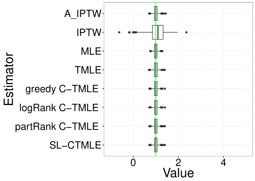
(a) Well specified model for $\bar{Q_{0}}$.

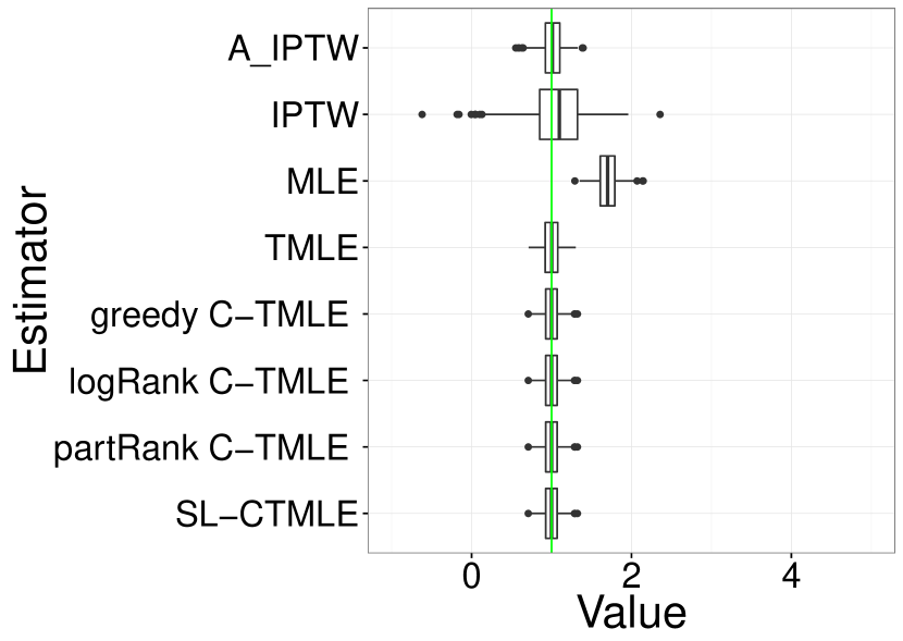
(b) Mis-specified model for $\bar{Q}_{0}$.

Figure 1: Simulation 1: Box plot of ATE estimates with correct/mis-specified models for $\bar{Q}_{0}$. The green line indicates the true parameter value.

Bias, variance, and mean squared error (MSE) for all estimators across 1000 simulated data sets are shown in Table 1. Box plots of the estimated ATE are shown in Fig. 1. When $Q_{0}$ was correctly specified, all models had very small bias. As Freedman and Berk discussed, even when the correct PS model is used, near positivity violations can lead to finite sample bias for IPTW estimators (see also Petersen et al., 2012). Scalable C-TMLEs had smaller bias than the other DR estimators, but the distinctions were small.

When $Q_{0}$ was not correctly specified, the G-computation/MLE estimator was expected to be biased. Interestingly, A-IPTW was more biased than the other DR estimators. All C-TMLE estimators have identical performance, because each approach produced the same treatment model sequence.

6.2 Simulation Study 2: Highly correlated covariates

In the second simulation study, we study the case that multiple confounders are highly correlated with each other. We will use the notation $W_{1:k}=(W_{1},\ldots,W_{k})$. The data-generating distribution is described as follows:

$$W_{1},W_{2},W_{3} \stackrel{{\scriptstyle iid}}{{\sim}} {\rm Bernoulli}(0.5),$$

$$W_{4}|W_{1:3} \sim {\rm Bernoulli}(0.2+0.5\cdot W_{1}),$$

$$W_{5}|W_{1:4} \sim {\rm Bernoulli}(0.05+0.3\cdot W_{1}+0.1\cdot W_{2}+0.05\cdot W_{3}+0.4\cdot W_{4}),$$

$$W_{6}|W_{1:5} \sim {\rm Bernoulli}(0.2+0.6\cdot W_{5}),$$

$$W_{7}|W_{1:6} \sim {\rm Bernoulli}(0.5+0.2\cdot W_{3}),$$

$$W_{8}|W_{1:7} \sim {\rm Bernoulli}(0.1+0.2\cdot W_{2}+0.3\cdot W_{6}+0.1\cdot W_{7}),$$

$$P_{0}(A=1\mid W) = g_{0}(1\mid W)$$

$$= \operatorname*{expit}(-0.05+0.1\cdot W_{1}+0.2\cdot W_{2}+0.2\cdot W_{3}$$

$$\qquad\qquad-0.02\cdot W_{4}-0.6\cdot W_{5}-0.2\cdot W_{6}-0.1\cdot W_{7}),$$

and finally, for $\epsilon\sim N(0,1)$ (independent from $A$ and $W$),

$$Y=10+A+W_{1}+W_{2}+W_{4}+2\cdot W_{6}+W_{7}+\epsilon.$$

The true ATE for this simulation study is $\psi_{0}=1$.

In this case, the true confounders are $W_{1},W_{2},W_{4},W_{6},W_{7}$. Covariate $W_{5}$ is most closely related to $W_{1}$ and $W_{4}$. Covariate $W_{3}$ is mainly associated with $W_{7}$. Neither $W_{3}$ nor $W_{5}$ is a confounder (both of them are predictive of treatment $A$, but do not influence directly outcome $Y$). Including either one of them in the PS model should inflate the variance (Brookhart et al., 2006).

As in Section 6.1, each of the estimators involving the estimation of $\bar{Q}_{0}$ was implemented twice, a correctly specified model to estimate $Q_{0}$, and a mis-specified model defined by a linear regression model of $Y$ on $A$ only.

Table 2: Simulation study 2. Performance of the various estimators across 1000 simulated data sets of sample size 1000.

	correct $\bar{Q}$			mis-specified $\bar{Q}$
	bias ($10^{-3}$)	se ($10^{-2}$)	MSE ($10^{-3}$)	bias ($10^{-3}$)	se ($10^{-2}$)	MSE ($10^{-3}$)
unadj	392.9	12.65	170.3	392.9	12.65	170.3
A_IPTW	2.4	6.54	4.3	2.0	6.53	4.3
IPTW	2.1	7.78	6.0	2.1	7.78	6.0
MLE	2.6	6.52	4.3	391.2	12.39	168.4
TMLE	2.4	6.54	4.3	2.0	6.53	4.3
greedy C-TMLE	2.6	6.52	4.3	11.4	7.01	5.0
logRank C-TMLE	2.5	6.52	4.3	6.3	6.72	4.6
partRank C-TMLE	2.6	6.52	4.3	2.5	6.67	4.4
SL-C-TMLE	2.5	6.52	4.3	5.2	6.79	4.6

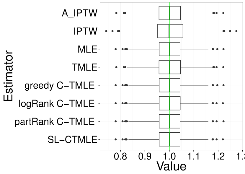
(a) Well specified model for $\bar{Q}_{0}$.

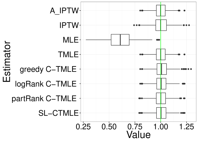
(b) Mis-specified model for $\bar{Q}_{0}$.

Figure 2: Simulation 2: Box plot of ATE estimates with correct/mis-specified models for $\bar{Q}_{0}$. The green line indicates the true parameter value.

Table 2 demonstrates and compares performance across 1000 replications. Box plots of the estimated ATE are shown in Fig. 2. When $\bar{Q}_{0}$ was correctly specified, all estimators except the unadjusted estimator had small bias. The DR estimators had lower MSE than the inefficient IPTW estimator. When $\bar{Q}_{0}$ was mis-specified, the A-IPTW and IPTW estimators were less biased than the C-TMLE estimators. The bias of the greedy C-TMLE was five times larger. However, all DR estimators had lower MSE than the IPTW estimator, with the TMLE outperforming the others.

6.3 Simulation Study 3: Binary outcome with instrumental variable

In the third simulation, we assess the performance of C-TMLE in a data set with positivity violations. We first generate $W_{1},W_{2},W_{3},W_{4}$ independently from the uniform distribution on $[0,1]$, then $A|W\sim{\rm Bernoulli}(g_{0}(1|W))$ with

$$g_{0}(1,W)=\operatorname*{expit}(-2+5W_{1}+2W_{2}+1W_{3}),$$

and finally $Y|(A,W)\sim{\rm Bernoulli}(\bar{Q}_{0}(A,W))$ with

$$\bar{Q}_{0}(A,W)=\operatorname*{expit}(-3+2W_{2}+2W_{3}+W_{4}+A).$$

As in Sections 6.1 and 6.2, each of the estimators involving the estimation of $\bar{Q}_{0}$ was implemented twice, once with a correctly specified model and once with a mis-specified linear regression model of $Y$ on $A$ only.

Table 3: Simulation study 3. Performance of the various estimators across 1000 simulated data sets of sample size 10000.

	correct $\bar{Q}$			mis-specified $\bar{Q}$
	bias ($10^{-3}$)	se ($10^{-2}$)	MSE ($10^{-3}$)	bias ($10^{-3}$)	se ($10^{-2}$)	MSE ($10^{-3}$)
unadj	78.1	3.72	7.5	78.1	3.72	7.5
A_IPTW	1.7	5.62	3.2	13.9	5.64	3.4
IPTW	45.9	6.05	5.8	45.9	6.05	5.8
MLE	0.7	4.20	1.8	76.4	3.61	7.1
TMLE	1.5	6.28	3.9	1.3	6.44	4.1
greedy C-TMLE	0.4	5.39	2.9	12.2	5.79	3.5
logRank C-TMLE	0.9	5.39	2.9	11.2	5.59	3.3
partRank C-TMLE	1.2	5.65	3.2	6.9	5.37	2.9
SL-C-TMLE	0.3	5.73	3.3	7.7	5.46	3.0

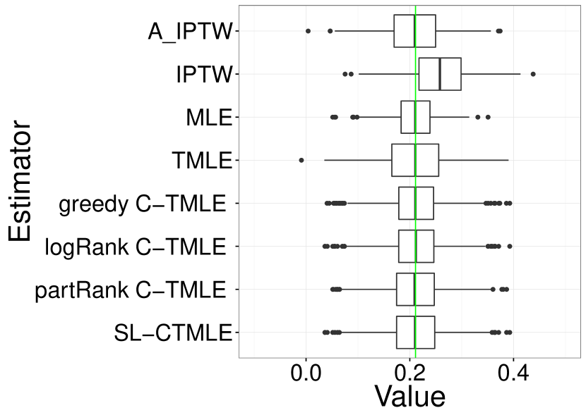
(a) Well specified model for $\bar{Q}_{0}$.

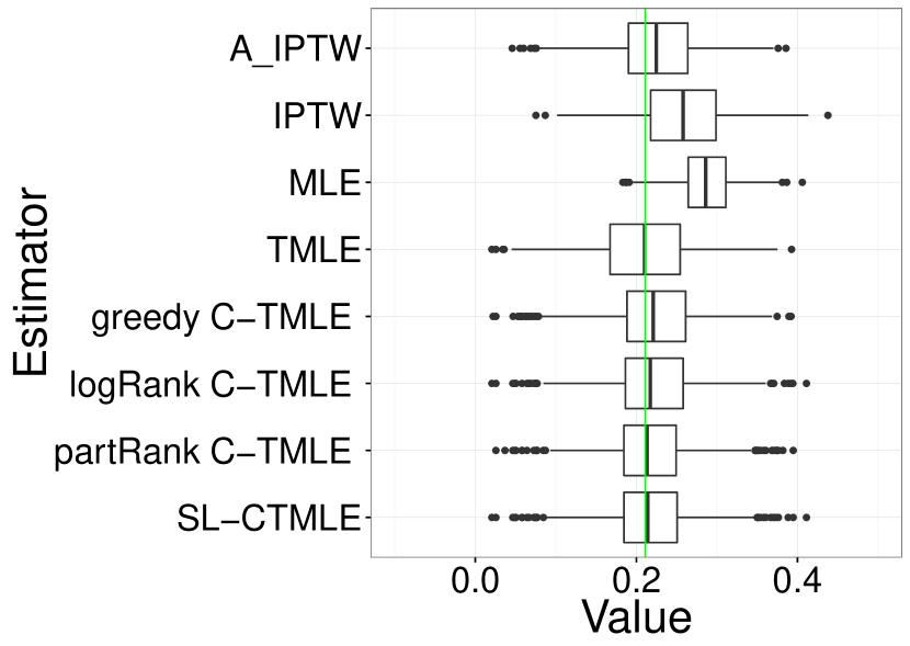
(b) Mis-specified model for $\bar{Q}_{0}$.

Figure 3: Simulation 3: Box plot of ATE estimates with correct/mis-specified models for $\bar{Q}_{0}$. The green line indicates the true parameter value.

Table 3 demonstrates the performance of the estimators across 1000 replications. Fig. 3 shows box plots of the estimates for the different methods across 1000 simulation, with a well specified or mis-specified model for $\bar{Q}_{0}$.

When $\bar{Q}_{0}$ was correctly specified, the DR estimators had similar bias/variance trade-offs. Although IPTW is a consistent estimator when $g$ is correctly specified, truncation of the PS $g_{n}$ may have introduced bias. However, without truncation it would have been extremely unstable due to violations of the positivity assumption when instrumental variables are included in the propensity score model.

When the model for $\bar{Q}_{0}$ was mis-specified, the MLE was equivalent to the unadjusted estimator. The DR methods performed well with an MSE close to that observed when $\bar{Q}_{0}$ was correctly specified. All C-TMLEs had similar performance. They out-performed the other DR methods (namely, A-IPTW and TMLE) and the pre-ordering strategies improved the computational time without loss of precision or accuracy compared to the greedy C-TMLE algorithm.

Side note.

Because $W_{1}$ is an instrumental variable that is highly predictive of the PS, but not helpful for confounding control, we expect that including it in the PS model would increase the variance of the estimator. One possible way to improve the performance of the IPTW estimator would be to apply a C-TMLE algorithm to select covariates for fitting the PS model. In the mis-specified model for $\bar{Q}_{0}$ scenario, we also simulated the following procedure:

1. Use a greedy C-TMLE algorithm to select the covariates.

2. Use main terms logistic regression with selected covariates for the PS model.

3. Compute IPTW using the estimated PS.

The simulated bias for this estimator was $0.0340$, the SE was $0.0568$, and the MSE was $0.0043$. Excluding the instrumental variable from the PS model thus reduced bias, variance, and MSE of the IPTW estimator.

6.4 Simulation Study 4: Continuous outcome with instrumental covariate

In the fourth simulation, we assess the performance of C-TMLEs in a simulation scheme with a continuous outcome inspired by (Gruber and van der Laan, 2011) (we merely increased the coefficient in front of $W_{1}$ to introduce a stronger positivity violation). We first independently draw $W_{1},W_{2},W_{3},W_{4},W_{5},W_{6}$ from the standard normal law, then $A$ given $W$ with

$$P_{0}(A=1\mid W)=g_{0}(1,W)=\operatorname*{expit}(2W_{1}+0.2W_{2}+-3W_{3}),$$

and finally $Y$ given $(A,W)$ from a Gaussian law with variance 1 and mean

$$\bar{Q}_{0}(A,W)=0.5W_{1}-8W_{2}+9W_{3}-2W_{5}+A.$$

The initial estimator $\bar{Q}_{n}^{0}$ was built based on a linear regression model of $Y$ on $A$, $W_{1}$, and $W_{2}$, thus partially adjusting for confounding. There was residual confounding due to $W_{3}$. There was also residual confounding due to $W_{1}$ and $W_{2}$ within at least one stratum of $A$, despite their inclusion in the initial outcome regression model.

Table 4: Simulation study 4. Performance of the various estimators across 1000 simulated data sets of sample size 1000. Omitted in the table, the performance of the unadjusted estimator was an order of magnitude worse than the performance of the other estimators.

	Mis-specified $\bar{Q}$
	bias	se	MSE
A_IPTW	4.49	0.84	20.88
IPTW	2.97	0.87	9.60
MLE	12.68	0.47	161.20
TMLE	1.31	1.21	3.17
greedy C-TMLE	0.25	1.01	1.27
logRank C-TMLE	0.36	0.88	0.90
partRank C-TMLE	0.32	0.92	0.95
SL-C-TMLE	0.37	0.88	0.90

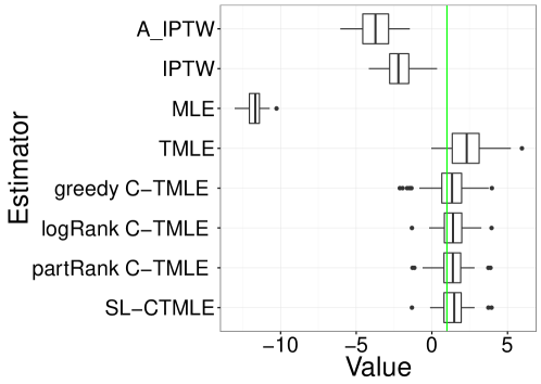
Figure 4: Simulation 4: Box plot of ATE estimates with mis-specified model for $\bar{Q}_{0}$.

Fig. 4 reveals that the C-TMLEs performed much better than TMLE and A-IPTW estimators in terms of bias and standard error. This illustrates that choosing to adjust for less than the full set of covariates can improve finite sample performance when there are near positivity violations. In addition, Table 4 shows that the pre-ordered C-TMLEs out-performed the greedy C-TMLE. Although the greedy C-TMLE estimator had smaller bias, it had higher variance, perhaps due to its more data-adaptive ordering procedure.

7 Simulation Study on Partially Synthetic Data

The aim of this section is to compare TMLE and all C-TMLEs using a large simulated data set that mimics a real-world data set. Section 7.1 starts the description of the data-generating scheme and resulting large data set. Section 7.2 presents the High-Dimensional Propensity Score (hdPS) method used to reduce the dimension of the data set. Section 7.3 completes the description of the data-generating scheme and specifies how $\bar{Q}_{0}$ and $g_{0}$ are estimated. Section 7.4 summarizes the results of the simulation study.

7.1 Data-generating scheme

The simulation scheme relies on the Nonsteroidal anti-inflammatory drugs (NSAID) data set presented and studied in (Schneeweiss et al., 2009, Rassen and Schneeweiss, 2012). Its $n=49,653$ observations were sampled from a population of patients aged 65 years and older, and enrolled in both Medicare and the Pennsylvania Pharmaceutical Assistance Contract for the Elderly (PACE) programs between 1995 and 2002. Each observed data structure consists of a triplet $(W,A,Y)$ where $W$ is decomposed in two parts: a vector of 22 baseline covariates and a highly sparse vector of $C=9,470$ unique claim codes. In the latter, each entry is a nonnegative integer indicating how many times (mostly zero) a certain procedure (uniquely identified among $C=9,470$ by its claim code) has been undergone by the corresponding patient. The claim codes were manually clustered into eight categories: ambulatory diagnoses, ambulatory procedures, hospital diagnoses, hospital procedures, nursing home diagnoses, physician diagnoses, physician procedures and prescription drugs. The binary indicator $A$ stands for exposure to a selective COX-2 inhibitor or a comparison drug (a non-selective NSAID). Finally, the binary outcome $Y$ indicates whether or not either a hospitalization for severe gastrointestinal hemorrhage or peptic ulcer disease complications including perforation in GI patients occurred.

The simulated data set was generated as in (Gadbury et al., 2008, Franklin et al., 2014). It took the form of $n=49,653$ data structures $(W_{i},A_{i},Y_{i})$ where $\{(W_{i},A_{i}):1\leq i\leq n\}$ was extracted from the above real data set and where $\{Y_{i}:1\leq i\leq n\}$ was simulated by us in such a way that, for each $1\leq i\leq n$, the random sampling of $Y_{i}$ depended only on the corresponding $(W_{i},A_{i})$. As argued in the aforementioned articles, this approach preserves the covariance structure of the covariates and complexity of the true treatment assignment mechanism, while allowing the true value of the ATE parameter to be known, and preserving control over the degree of confounding.

7.2 High-Dimensional Propensity Score Method For Dimension Reduction

The simulated data set was large, both in number of observations and the number of covariates. In this framework, directly applying any version of C-TMLE algorithms would not be the best course of action First, the computational time would be unreasonably long due to the large number of covariates. Second, the resulting estimators would be plagued by high variance due to the low signal-to-noise ratio in the claim data.

This motivated us to apply the High-Dimensional Propensity Score (hdPS) method for dimension reduction prior to applying the TMLE and C-TMLE algorithms.

Introduced in (Schneeweiss et al., 2009)), the hdPS method was proposed to reduce the dimension in large electronic healthcare databases. It is is increasingly used in studies involving such databases (Rassen and Schneeweiss, 2012, Patorno et al., 2014, Franklin et al., 2015, Toh et al., 2011, Kumamaru et al., 2016, Ju et al., 2016)).

The hdPS method essentially consists of two main steps: (i) generating so called hdPS covariates from the claims data (which can increase the dimension) then (ii) screening the enlarged collection of covariates to select a small proportion of them (which dramatically reduces the dimension). Specifically, the method unfolds as follows (Schneeweiss et al., 2009):

1. Cluster by Resource.

Cluster the data by resource in ${\cal C}$ clusters.

In the current example, we derived ${\cal C}=8$ clusters corresponding to the following categories: ambulatory diagnoses, ambulatory procedures, hospital diagnoses, hospital procedures, nursing home diagnoses, physician diagnoses, physician procedures and prescription drugs. See (Schneeweiss et al., 2009, Patorno et al., 2014) for other examples.

2. Identify Candidate Claim Codes.

For each cluster separately, for each claim code $c$ within the cluster, compute the empirical proportion $Pr(c)$ of positive entries, then sort the claim codes by decreasing values of $\min(Pr(c),1-Pr(c))$. Finally, select only the top $J$ claim codes. We thus go from $C$ claim codes to $J\times{\cal C}$ claim codes.

As explained below, we chose $J=50$ so the dimension of the claims data went from $9,470$ to 400.

3. Assess Recurrence of Claim Codes.

For each selected claim code $c$ and each patient $1\leq i\leq n$, replace the corresponding $c_{i}$ with three binary covariates called “hdPS covariates”: $c_{i}^{(1)}$ equal to one if and only if (iff) $c_{i}$ is positive; $c_{i}^{(2)}$ equal to one iff $c_{i}$ is larger than the median of $\{c_{i}:1\leq i\leq n\}$; $c_{i}^{(3)}$ equal to one iff $c_{i}$ is larger than the 75%-quantile of $\{c_{i}:1\leq i\leq n\}$. This inflates the number of claim codes related covariates by a factor 3.

As explained below, the dimension of the claims data thus went from 400 to $1,200$.

4. Select Among the hdPS Covariates.

For each hdPS covariate, estimate a measure of its potential confounding impact, then sort them by decreasing values of the estimates of the measure. Finally, select only the top $K$ hdPS covariates.

For instance, one can rely on the following estimate of the measure of the potential confounding impact introduced in (Bross, 1954): for hdPS covariate $c^{\ell}$

$$\frac{\pi_{n}^{\ell}(1)(r_{n}^{\ell}-1)+1}{\pi_{n}^{\ell}(0)(r_{n}^{\ell}-1)+1}$$ (9)

where

$$\pi_{n}^{\ell}(a) = \frac{\sum_{i=1}^{n}{\bf 1}\{c_{i}^{\ell}=1,a_{i}=a\}}{\sum_{i=1}^{n}{\bf 1}\{a_{i}=a\}}\quad(a=0,1)\quad\text{and}$$

$$r_{n}^{\ell} = \frac{p_{n}(1)}{p_{n}(0)}\quad\text{with}\quad p_{n}(c)=\frac{\sum_{i=1}^{n}{\bf 1}\{y_{i}=1,c_{i}^{\ell}=c\}}{\sum_{i=1}^{n}{\bf 1}\{c_{i}^{\ell}=c\}}\quad(c=0,1).$$

A rationale for this choice can be found in (Schneeweiss et al., 2009), where $r_{n}^{\ell}$ in (9) is replaced by $\max(r_{n}^{\ell},1/r_{n}^{\ell})$.

As explained below we chose $K=100$. As a result, the dimension of the claims data was reduced to 100 from $9,470$.

7.3 Data-generating scheme (continued) and estimating procedures

Let us resume here the presentation of the simulation scheme initiated in Section 7.1. Recall that the simulated data set writes as $\{(W_{i},A_{i},Y_{i}):1\leq i\leq n\}$ where $\{W_{i}:1\leq i\leq n\}$ is the by product of the hdPS method of Section 7.2 with $J=50$ and $K=100$ and $\{A_{i}:1\leq i\leq n\}$ is the original vector of exposures. It only remains to present how $\{Y_{i}:1\leq i\leq n\}$ was generated.

First, we arbitrarily chose a subset $W^{\prime}$ of $W$, that consists of 10 baseline covariates (congestive heart failure, previous use of warfarin, number of generic drugs in last year, previous use of oral steroids, rheumatoid arthritis, age in years, osteoarthritis, number of doctor visits in last year, calendar year) and 5 hdPS covariates. Second, we arbitrarily defined a parameter

$$\beta=(1.280,-1.727,1.690,0.503,2.528,0.549,0.238,-1.048,1.294,\\ 0.825,-0.055,-0.784,-0.733,-0.215,-0.334)^{\top}.$$

Finally, $Y_{1},\ldots,Y_{n}$ were independently sampled given $\{(W_{i},A_{i}):1\leq i\leq n\}$ from Bernoulli distributions with parameters $q_{1},\ldots,q_{n}$ where, for each $1\leq i\leq n$,

$$q_{i}=\operatorname*{expit}\left(\beta^{\top}W_{i}^{\prime}+A_{i}\right).$$

The resulting true value of the ATE is $\psi_{0}=0.21156$.

The estimation of the conditional expectation $\bar{Q}_{0}$ was carried out based on two logistic regression models. The first one was well specified whereas the second one was mis-specified, due to the omission of the five hdPS covariates.

For the TMLE algorithm, the estimation of the PS $g_{0}$ was carried out based on a single, main terms logistic regression model including all of the 122 covariates. For the C-TMLE algorithms, main terms logistic regression model were also fitted at each step. An early stopping rule was implemented to save computational time. Specifically, if the cross-validated loss of $\bar{Q}_{n,k}^{*}$ is smaller than the cross-validated losses of $\bar{Q}_{n,k+1}^{*},\ldots,\bar{Q}_{n,k+10}^{*}$, then the procedure is stopped and outputs the TMLE estimator corresponding to $\bar{Q}_{n,k}^{*}$.

The scalable SL-C-TMLE library included the two scalable pre-ordered C-TMLE algorithms and excluded the greedy C-TMLE algorithm.

7.4 Results

Table 5 reports the point estimates for $\psi_{0}$ as derived by all the considered methods. It also reports the 95% CIs of the form $[\psi_{n}\pm 1.96\sigma_{n}/\sqrt{n}]$, where $\sigma_{n}^{2}=n^{-1}\sum_{i=1}^{n}D^{*}(\bar{Q}_{n},g_{n})(O_{i})^{2}$ estimates the variance of the efficient influence curve at the couple $(\bar{Q}_{n},g_{n})$ yielding $\psi_{n}$. We refer the interested reader to (van der Laan and Rose, 2011, Appendix A) for details on influence curve based inference. All the CIs contained the true value of $\psi_{0}$. Table 5 also reports processing times (in seconds).

Table 5: Point estimates and 95% CIs for TMLE and C-TMLE estimators

	Model for $\bar{Q}_{n}^{0}$	estimate	CI	Processing time
TMLE	Well specified	0.202	(0.193, 0.212)	0.6s
	Mis-specified	0.203	(0.193, 0.213)	0.6s
C-TMLE,	Well specified	0.205	(0.196, 0.213)	618.7s
greedy	Mis-specified	0.214	(0.205, 0.223)	1101.2s
C-TMLE,	Well specified	0.205	(0.196, 0.213)	57.4s
logistic ordering	Mis-specified	0.211	(0.202, 0.219)	125.6s
C-TMLE,	Well specified	0.205	(0.197, 0.213)	22.5s
partial correlation ordering	Mis-specified	0.211	(0.202, 0.219)	149.0s
SL-C-TMLE	Well specified	0.205	(0.197, 0.213)	69.8s
	Mis-specified	0.211	(0.202, 0.219)	264.3s

The point estimates and CIs were similar across all C-TMLEs. When the model for $\bar{Q}_{0}$ was correctly specified, the SL-C-TMLE selected the partial correlation ordering. When the model for $\bar{Q}_{0}$ was mis-specified, it selected the logistic ordering. In both cases, the estimator with smaller bias was data-adaptively selected. In addition, as all the candidates in its library were scalable, the SL-C-TMLE algorithm was also scalable, and ran much faster than the greedy C-TMLE algorithm. Computational time for the scalable C-TMLE algorithms was approximately 1/10th of the computational time of the greedy C-TMLE algorithm.

8 Discussion

Robust inference of a low-dimensional parameter in a large semi-parametric model traditionally relies on external estimators of infinite-dimensional features of the distribution of the data. Typically, only one of the latter is optimized for the sake of constructing a well behaved estimator of the low-dimensional parameter of interest. For instance, the targeted minimum loss (TMLE) estimator of the average treatment effect (ATE) (2) relies on an external estimator $\bar{Q}_{n}^{0}$ of the conditional mean $\bar{Q}_{0}$ of the outcome given binary treatment and baseline covariates, and on an external estimator $g_{n}$ of the propensity score $g_{0}$. Only $\bar{Q}_{n}^{0}$ is optimized/updated into $\bar{Q}_{n}^{*}$ based on $g_{n}$ in such a way that the resulting substitution estimator of the ATE can be used, under mild assumptions, to derive a narrow confidence interval with a given asymptotic level.

There is room for optimization in the estimation of $g_{0}$ for the sake of achieving a better bias-variance trade-off in the estimation of the ATE. This is the core idea driving the general C-TMLE template. It uses a targeted penalized loss function to make smart choices in determining which variables to adjust for in the estimation of $g_{0}$, only adjusting for variables that have not been fully exploited in the construction of $\bar{Q}_{n}^{0}$, as revealed in the course of a data-driven sequential procedure.

The original instantiation of the general C-TMLE template was presented as a greedy forward stepwise algorithm. It does not scale well when the number $p$ of covariates increases drastically. This motivated the introduction of novel instantiations of the C-TMLE general template where the covariates are pre-ordered. Their time complexity is $\mathcal{O}(p)$ as opposed to the original $\mathcal{O}(p^{2})$, a remarkable gain. We proposed two pre-ordering strategies and suggested a rule of thumb to develop other meaningful strategies. Because it is usually unclear a priori which pre-ordering strategy to choose, we also introduced a SL-C-TMLE algorithm that enables the data-driven choice of the better pre-ordering given the problem at hand. Its time complexity is $\mathcal{O}(p)$ as well.

The C-TMLE algorithms used in our data analyses have been implemented in Julia and are publicly available at https://lendle.github.io/TargetedLearning.jl/. We undertook five simulation studies. Four of them involved fully synthetic data. The last one involves partially synthetic data based on a real electronic health database and the implementation of a high-dimensional propensity score (hdPS) method for dimension reduction widely used for the statistical analysis of claim codes data. In the appendix, we compare the computational times of variants of C-TMLE algorithms. We also showcase the use of C-TMLE algorithms on three real electronic health database. In all analyses involving electronic health databases, the greedy C-TMLE algorithm was unacceptably slow. Judging from the simulation studies, our scalable C-TMLE algorithms work well, and so does the SL-C-TMLE algorithm.

This article focused on ATE with a binary treatment. In future work, we will adapt the theory and practice of scalable C-TMLE algorithms for the estimation of the ATE with multi-level or continuous treatment by employing a working marginal structural model. We will also extend the analysis to address the estimation of other classical parameters of interest.

Appendix

We gather here some additional material. Appendix A provides notes on a Julia software package that implements all the proposed C-TMLE algorithms. Appendix B presents and compares the empirical processing time of C-TMLE algorithms for different sample sizes and number of candidate estimators of the nuisance parameter. Appendix C compares the performance of the new C-TMLEs with standard TMLE on three real data sets.

Appendix A C-TMLE Software

A flexible Julia software package implementing all C-TMLE algorithms described in this article is publicly available at https://lendle.github.io/TargetedLearning.jl/. The website contains detailed documentation and a tutorial for researchers who do not have experience with Julia.

In addition to the two pre-ordering methods described in Section 5, the software accepts any user-defined ranking algorithm. The software also offers several options to decrease the computational time of the scalable C-TMLE algorithms. The "Pre-Ordered" search strategy has an optional argument k which defaults to 1. At each step, the next $k$ available ordered covariates are added to the model used to estimate $g_{0}$. Large $k$ can speed up the procedure when there are many covariates. However, this approach is prone to over-fitting, and may miss the optimal solution.

An early stopping criteria that avoids computing and cross-validating the complete model containing all $p$ covariates can also save unnecessary computations. A "patience" argument accelerates the training phase by setting the number of steps to carry out after having found a local optimum. To prepare Section 7.1, argument "patience" was set to 10. More details are provided in that section.

Appendix B Time Complexity

We study here the computational time of the pre-ordered C-TMLE algorithms. The computational time of each algorithm depends on the sample size $n$ and number of covariates $p$. First, we set $n=1,000$ and varied $p$ between 10 and 100 by steps of 10. Second, we varied $n$ from $1,000$ to $20,000$ by steps of $1,000$ and set $p=20$. For each $(n,p)$ pair, the analysis was replicated ten times independently, and the median computational time was reported. In every data set, all the random variables are mutually independent. The results are shown in Figures 5(a) and 5(b).

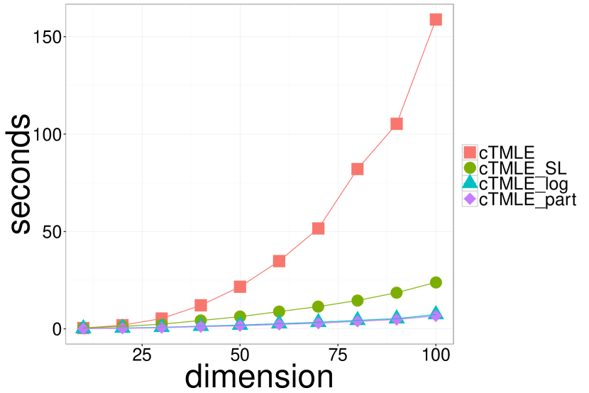
(a) Median computational time (across 10 replications for each point), with $n=1,000$ fixed and $p$ varying.

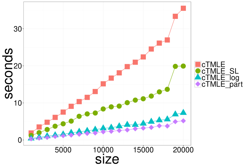
(b) Median computational time (across 10 replications for each point), with varying $n$ and fixed $p=20$.

Figure 5: Computational times of the C-TMLE algorithms with greedy search and pre-ordering.

Figure 5(a) is in line with the theory: the computational time of the forward stepwise C-TMLE is $\mathcal{O}(p^{2})$ whereas the computational times of the pre-ordered C-TMLE algorithms are $\mathcal{O}(p)$. Note that the pre-ordered C-TMLEs are indeed scalable. When $n=1,000$ and $p=100$, all the scalable C-TMLE algorithms ran in less than 30 seconds.

Figure 5(b) reveals that the pre-ordered C-TMLE algorithms are much faster in practice than the greedy C-TMLE algorithm, even if all computational times are $\mathcal{O}(n)$ in that framework with fixed $p$.

Appendix C Real Data Analyses

This section presents the application of variants of the TMLE and C-TMLE algorithms for the analysis of three real data sets. Our objectives are to showcase their use and to illustrate the consistency of the results provided by the scalable and greedy C-TMLE estimators. We thus do not implement the competing unadjusted, G-computation/MLE, IPTW and A-IPTW estimators (see the beginning of Section 6).

In Sections 6 and 7, we knew the true value of the ATE. This is not the case here.

C.1 Real data sets and estimating procedures

We compared the performance of variants of TMLE and C-TMLE algorithms across three observational data sets. Here are brief descriptions, borrowed from Schneeweiss et al. (2009), Ju et al. (2016).

NSAID Data Set.

Refer to Section 7.1 for its description.

Novel Oral Anticoagulant (NOAC) Data Set.

The NOAC data were collected between October, 2009 and December, 2012 by United Healthcare. The data set tracked a cohort of new users of oral anticoagulants for use in a study of the comparative safety and effectiveness of these agents. The exposure is either “warfarin” or “dabigatran”. The binary outcome indicates whether or not a patient had a stroke during the 180 days after initiation of an anticoagulant.

The data set includes $n=18,447$ observations, $p=60$ baseline covariates and $C=23,531$ unique claim codes. The claim codes are manually clustered in four categories: inpatient diagnoses, outpatient diagnoses, inpatient procedures and outpatient procedures.

Vytorin Data Set.

The Vytorin data included all United Healthcare patients who initiated either treatment between January 1, 2003 and December 31, 2012, with age over 65 on day of entry into cohort. The data set tracked a cohort of new users of Vytorin and high-intensity statin therapies. The exposure is either “Vytorin” or “high-intensity statin”. The outcomes indicates whether or not any of the events “myocardial infarction”, “stroke” and “death” occurred.

The data set includes $n=148,327$ observations, $p=67$ baseline covariates and $C=15,010$ unique claim codes. The claim codes are manually clustered in five categories: ambulatory diagnoses, ambulatory procedures, hospital diagnoses, hospital procedures, and prescription drugs.

Each data set is given by $\{(W_{i},A_{i},Y_{i}):1\leq i\leq n\}$ where $\{W_{i}:1\leq i\leq n\}$ is the by product of the hdPS method of Section 7.2 with $J=100$ and $K=200$ and $\{(A_{i},Y_{i}):1\leq i\leq n\}$ is the original collection of paired exposures and outcomes.

The estimations of the conditional expectation $\bar{Q}_{0}$ and of the PS $g_{0}$ were carried out based on logistic regression models. Both models used either the baseline covariates only or the baseline covariates and the additional hdPS covariates.

To save computational time, the C-TMLE algorithms relied on the same early stopping rule described in Section 7.3. The scalable SL-C-TMLE library included the two scalable pre-ordered C-TMLE algorithms and excluded the greedy C-TMLE algorithm.

C.2 Results on the NSAID data set

Figure 6 shows the point estimates and 95% CIs yielded by the different TMLE and C-TMLE estimators built from the NSAID data set.

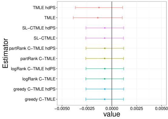
Figure 6: Point estimates and 95% CIs yielded by the different TMLE and C-TMLE estimators built on the NSAID data set.

The various C-TMLE estimators exhibit similar results, with slightly larger point estimates and narrower CIs compared to the TMLE estimators. All the CIs contain zero.

C.3 Results on the NOAC Data Set

Figure 7 shows the point estimates and 95% CIs yielded by the different TMLE and C-TMLE estimators built on the NOAC data set.

We observe more variability in the results than in those presented in Appendix C.2.

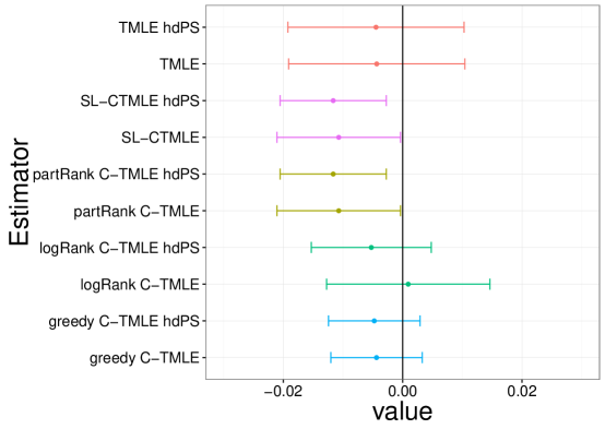
Figure 7: Point estimates and 95% CIs yielded by the different TMLE and C-TMLEs built on the NOAC data set.

The various TMLE and C-TMLEs exhibit similar results, with a non-significant shift to the right for the latter. All the CIs contain zero.

C.4 Results on the Vytorin Data Set

Figure 8 shows the point estimates and 95% CIs yielded by the different TMLE and C-TMLEs built on the Vytorin data set.

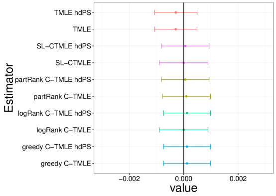
Figure 8: Point estimates and 95% CIs yielded by the different TMLE and C-TMLEs built on the Vytorin data set.

The various TMLE and C-TMLEs exhibit similar results, with a non-significant shift to the right for the latter. All the CIs contain zero.

References

- Bickel et al. (1998) Bickel, P. J., C. A. Klaassen, Y. Ritov, J. A. Wellner, et al. (1998): Efficient and adaptive estimation for semiparametric models, Springer-Verlag.
- Brookhart et al. (2006) Brookhart, M. A., S. Schneeweiss, K. J. Rothman, R. J. Glynn, J. Avorn, and T. Stürmer (2006): “Variable selection for propensity score models,” American Journal of Epidemiology, 163, 1149–1156.
- Bross (1954) Bross, I. (1954): “Misclassification in 2 x 2 tables,” Biometrics, 10, 478–486.
- Franklin et al. (2015) Franklin, J. M., W. Eddings, R. J. Glynn, and S. Schneeweiss (2015): “Regularized regression versus the high-dimensional propensity score for confounding adjustment in secondary database analyses,” American journal of epidemiology, 187, 651–659.
- Franklin et al. (2014) Franklin, J. M., S. Schneeweiss, J. M. Polinski, and J. A. Rassen (2014): “Plasmode simulation for the evaluation of pharmacoepidemiologic methods in complex healthcare databases,” Computational Statistics & Data Analysis, 72, 219–226.
- Freedman and Berk (2008) Freedman, D. A. and R. A. Berk (2008): “Weighting regressions by propensity scores,” Evaluation Review, 32, 392–409.
- Gadbury et al. (2008) Gadbury, G. L., Q. Xiang, L. Yang, S. Barnes, G. P. Page, and D. B. Allison (2008): “Evaluating statistical methods using plasmode data sets in the age of massive public databases: an illustration using false discovery rates,” PLoS Genet, 4, e1000098.
- Gruber and van der Laan (2010a) Gruber, S. and M. J. van der Laan (2010a): “An application of collaborative targeted maximum likelihood estimation in causal inference and genomics,” The International Journal of Biostatistics, 6, Article 18.
- Gruber and van der Laan (2010b) Gruber, S. and M. J. van der Laan (2010b): “A targeted maximum likelihood estimator of a causal effect on a bounded continuous outcome,” The International Journal of Biostatistics, 6, Article 26.
- Gruber and van der Laan (2011) Gruber, S. and M. J. van der Laan (2011): “C-tmle of an additive point treatment effect,” in Targeted Learning, Springer, 301–321.
- Hair et al. (2006) Hair, J. F., W. C. Black, B. J. Babin, R. E. Anderson, and R. L. Tatham (2006): Multivariate Data Analysis, volume 6, Pearson Prentice Hall Upper Saddle River, NJ.
- Hernan et al. (2000) Hernan, M. A., B. Brumback, and J. M. Robins (2000): “Marginal structural models to estimate the causal effect of zidovudine on the survival of HIV-positive men,” Epidemiology, 11, 561–570.
- Ju et al. (2016) Ju, C., M. Combs, S. D. Lendle, J. M. Franklin, R. Wyss, S. Schneeweiss, and M. J. van der Laan (2016): “Propensity score prediction for electronic healthcare dataset using super learner and high-dimensional propensity score method,” , U.C. Berkeley Division of Biostatistics Working Paper Series. Working Paper 351. http://biostats.bepress.com/ucbbiostat/paper351.
- Kumamaru et al. (2016) Kumamaru, H., J. J. Gagne, R. J. Glynn, S. Setoguchi, and S. Schneeweiss (2016): “Comparison of high-dimensional confounder summary scores in comparative studies of newly marketed medications,” Journal of clinical epidemiology, 76, 200–208.
- Patorno et al. (2014) Patorno, E., R. J. Glynn, S. Hernández-Díaz, J. Liu, and S. Schneeweiss (2014): “Studies with many covariates and few outcomes: selecting covariates and implementing propensity-score–based confounding adjustments,” Epidemiology, 25, 268–278.
- Petersen et al. (2012) Petersen, M. L., K. E. Porter, S. Gruber, Y. Wang, and M. J. van der Laan (2012): “Diagnosing and responding to violations in the positivity assumption,” Statistical methods in medical research, 21, 31–54.
- Porter et al. (2011) Porter, K. E., S. Gruber, M. J. van der Laan, and J. S. Sekhon (2011): “The relative performance of targeted maximum likelihood estimators,” The International Journal of Biostatistics, 7, Article 31.
- Rassen and Schneeweiss (2012) Rassen, J. A. and S. Schneeweiss (2012): “Using high-dimensional propensity scores to automate confounding control in a distributed medical product safety surveillance system,” Pharmacoepidemiology and drug safety, 21, 41–49.
- Robins (2000a) Robins, J. (2000a): “Robust estimation in sequentially ignorable missing data and causal inference models,” in Proceedings of the American Statistical Association: Section on Bayesian Statistical Science, 6–10.
- Robins (1986) Robins, J. M. (1986): “A new approach to causal inference in mortality studies with sustained exposure periods - application to control of the healthy worker survivor effect,” Mathematical Modelling, 7, 1393–1512.
- Robins (2000b) Robins, J. M. (2000b): “Marginal structural models versus structural nested models as tools for causal inference,” in Statistical models in epidemiology, the environment, and clinical trials, Springer, 95–133.
- Robins et al. (2000a) Robins, J. M., M. A. Hernan, and B. Brumback (2000a): “Marginal structural models and causal inference in epidemiology,” Epidemiology, 11, 550–560.
- Robins and Rotnitzky (2001) Robins, J. M. and A. Rotnitzky (2001): “Comment on the Bickel and Kwon article, ‘Inference for semiparametric models: Some questions and an answer’,” Statistica Sinica, 11, 920–936.
- Robins et al. (2000b) Robins, J. M., A. Rotnitzky, and M. van der Laan (2000b): “Comment on “On Profile Likelihood” by S.A. Murphy and A.W. van der Vaart,” Journal of the American Statistical Association – Theory and Methods, 450, 431–435.
- Robins et al. (1994) Robins, J. M., A. Rotnitzky, and L. P. Zhao (1994): “Estimation of regression coefficients when some regressors are not always observed,” Journal of the American statistical Association, 89, 846–866.
- Schneeweiss et al. (2009) Schneeweiss, S., J. A. Rassen, R. J. Glynn, J. Avorn, H. Mogun, and M. A. Brookhart (2009): “High-dimensional propensity score adjustment in studies of treatment effects using health care claims data,” Epidemiology, 20, 512.
- Stitelman and van der Laan (2010) Stitelman, O. M. and M. J. van der Laan (2010): “Collaborative targeted maximum likelihood for time to event data,” The International Journal of Biostatistics, 6, Article 21.
- Stitelman et al. (2011) Stitelman, O. M., C. W. Wester, V. De Gruttola, and M. J. van der Laan (2011): “Targeted maximum likelihood estimation of effect modification parameters in survival analysis,” The International Journal of Biostatistics, 7, Article 19.
- Toh et al. (2011) Toh, S., L. A. García Rodríguez, and M. A. Hernán (2011): “Confounding adjustment via a semi-automated high-dimensional propensity score algorithm: an application to electronic medical records,” Pharmacoepidemiology and drug safety, 20, 849–857.
- van der Laan and Dudoit (2003) van der Laan, M. J. and S. Dudoit (2003): “Unified cross-validation methodology for selection among estimators and a general cross-validated adaptive epsilon-net estimator: Finite sample oracle inequalities and examples,” , U.C. Berkeley Division of Biostatistics Working Paper Series. Working Paper 130. http://works.bepress.com/sandrine_dudoit/34/.
- van der Laan and Gruber (2010) van der Laan, M. J. and S. Gruber (2010): “Collaborative double robust targeted maximum likelihood estimation,” The International Journal of Biostatistics, 6, Article 17.
- van der Laan et al. (2007) van der Laan, M. J., E. C. Polley, and A. E. Hubbard (2007): “Super learner,” Statistical Applications in Genetics and Molecular Biology, 6, Article 25.
- van der Laan and Rose (2011) van der Laan, M. J. and S. Rose (2011): Targeted Learning: Causal Inference for Observational and Experimental Data, Springer Science & Business Media.
- van der Laan and Rubin (2006) van der Laan, M. J. and D. Rubin (2006): “Targeted maximum likelihood learning,” The International Journal of Biostatistics, 2.
- van der Vaart et al. (2006) van der Vaart, A. W., S. Dudoit, and M. J. Laan (2006): “Oracle inequalities for multi-fold cross validation,” Statistics & Decisions, 24, 351–371.
- Wang et al. (2011) Wang, H., S. Rose, and M. J. van der Laan (2011): “Finding quantitative trait loci genes with collaborative targeted maximum likelihood learning,” Statistics & Probability Letters, 81, 792–796.