Abstract

Within the MSSM, we have evaluated the decay rates for the lepton flavour violating Higgs boson decays (LFVHD) $h\rightarrow l_{i}l_{j}$ where $l_{i,j}$ are charged leptons and $i\neq j$. This has been done in a model independent (MI) way as well as in supersymmetric high scale seesaw models, in particular Type I see-saw model. Lepton flavour violation (LFV) is generated by non-diagonal entries in the mass matrix of the sleptons. In a first step we use the model independent approach where LFV (off-diagonal entries in the mass matrix) is introduced by hand while respecting the direct search constraints from the charged lepton flavor violating (cLFV) processes. In the second step we use high scale see-saw models where LFV is generated via renormalization group equations (RGE) from the grand unification scale (GUT) down to electroweak scale. cLFV decays are the most restrictive ones and exclude a large part of the parameter space for the MI as well as the high scale see-saw scenarios. Due to very strict constraints from cLFV, it is difficult to find large corrections to LFVHD. This applies in particular to $h\rightarrow\tau\mu$ where hints of an excess have been observed. If this signal is confirmed, it could not be explained with the models under investigation.

1 Introduction

The Standard Model (SM) predicts flavor mixing in the quark sector. However, lepton flavor violation (LFV) is exactly zero due to the assumption of vanishing neutrino masses. The observation of neutrino oscillations[1] certainly contradicts the SM, and also suggest the possibilty of the observation of flavour violation on the chaged sector (cLFV). However, processes such as $l_{i}\rightarrow l_{j}\gamma$, with $i\neq j$ and $l_{i,j}=e,\mu,\tau$ have not been observed yet. Even if the SM is complemented with massive non-degenerate light neutrinos, the rates for these processes are supressed by a factor $\Delta m_{\nu}^{4}/M_{W}^{4}$ where $\Delta m_{\nu}$ denotes the neutrino mass splitting and $M_{W}$ the $W$ boson mass. Data from neutrino oscillations implies values for $\Delta m_{\nu}$ so small that the processes like BR($l_{i}\rightarrow l_{j}\gamma$) would be out of the experimental scope. Independently of the neutrino problem, even the Minimal Supersymetric Standard Model (MSSM) [2] can predict charged LFV due to flavor mixing in the sleptons (scalar partners of the leptons) allowing prediction for these process in the experimental reach [3, 4]. The same mechanism can enable LFV Higgs decays, such decays have gathered a lot of attention after CMS reported excess for the channel $h\rightarrow\mu\tau$ [5]. This seems to be consistent with the latest analysis of the ATLAS results [6]. However, their significance is not large enough and further data is needed to confirm or exclude this excess.

The complementation of the MSSM with a mechanism to explain neutrino oscillations can relate those to corresponding cLFV effects. A first guess would be to write down the neutrino yukawa couplings which generates neutrino masses via electroweak symmetry breaking (EWSB). However those couplings will be so small that it will be very difficult to link them to the observation of cLFV. This picture changes when these masses are explained with a “see-saw” mechanism [7], that can be implemented in different ways [8, 9]. The most popular of these mechanisms is Type-I see-saw[7], the small neutrino mass $m_{\nu}\approx Y_{\nu}^{2}v^{2}/M_{R}$ with $Y_{\nu}$ the neutrino yukawa coupling, $M_{R}$ the seesaw scale and $v$ the vacuum expectation value, is achieved with a high scale $M_{R}$ which can allow large values for $Y_{\nu}$. Even with the assumption of universal soft masses at the GUT scale, the presence of $Y_{\nu}$ in the RGE above $M_{R}$ can generate non trivial slepton mixings, hence relating cLFV to the neutrino problem [10, 11, 12, 13, 14, 15, 16, 17, 18, 19, 20, 21, 22, 23, 24] and GUT scenarios [25, 26, 27, 28]. Other popular high scale seesaw mechanisms are Type II [29, 30] and Type III [31, 32] seesaw models. In Type II seesaw, the heavy particle is a Higgs triplet, whereas in Type III see-saw model, the exchanged particle should be a right-handed fermion triplet. At low energy, the neutrino masses are generated by a dimension 5 operator and one can not distinguish between different see-saw realizations. One common feature among these models is that the LFV effects in these models are generated by non diagonal entries (as explained above for the Type I see-saw mechanism) in the slepton mass matrix. These off-diagonal entries in the slepton mass matrix not only predict sizeable rates for the cLFV processes but can also results in the LFV decays of the Higgs boson [33, 34, 35, 36, 37, 38, 39]. While supersymmetric high scale see-saw models successfully describe the neutrino masses and mixing and predict sizeable rates for the cLFV processes, it is yet to be seen if they can also explain the CMS reported excess, which precisely is the aim of this work.

In this article we evaluate LFV Higgs decays like $h\rightarrow l_{i}l_{j}$ where $l_{i,j=e,\mu,\tau}$ are the charged leptons with $i\neq j$. For our calculations we prepared an add-on model file for FeynArts [40, 41] which adds LFV effects to the existing MSSM model file, as described in [42, 43]. We carry out our numerical analysis in two frameworks. In the first framework we study several expamples of mass spectra for the MSSM consistent with all the phenomenological constraints. Flavor mixing is generated by putting off-diagonal enteries in the slepton mass matrices by hand such that cLFV is consistent with direct experimental searches. In the second framework, we study MSSM augmented by the high scale seesaw models in particular Type I seesaw mechanism[7] and flavor mixing is generated through RGEs as explained above.

This paper is organised in the following way: In section 2 the MSSM is presented and we introduce our definitions of the slepton basis and mass matrices. The third section is dedicated to briefly review the observables that will be studied in this paper. In the fourth section we present our numerical analysis in the MI approach for the observables of section 3. In section 5 we present our numerical analysis for the MSSM augmented by seesaw Type I mechanism. Finally, our conclusions can be found in section 6.

2 LFV in the MSSM

The MSSM is the most popular SUSY extension of the SM. With the assumption of soft SUSY breaking terms we introduce a flavor mismatch for the scalar partners with respect to their corresponding leptons. Therefore, flavor violation is introduced through loops containing SUSY particles. In this section, along with the MSSM we introduce the definitions and operational basis that will be used in the rest of the work. We use the same notation as in Refs. [37, 44, 38, 43, 45].

One can write the most general $SU(3)_{C}\times SU(2)_{L}\times U(1)_{Y}$ gauge invariant and renormalizable R-parity conserving superpotential for the MSSM as

$$W_{\rm MSSM} = Y_{e}^{ij}\epsilon_{\alpha\beta}H_{1}^{\alpha}E_{i}^{c}L_{j}^{\beta}+Y_{d}^{ij}\epsilon_{\alpha\beta}H_{1}^{\alpha}D_{i}^{c}Q_{j}^{\beta}+Y_{u}^{ij}\epsilon_{\alpha\beta}H_{2}^{\alpha}U_{i}^{c}Q_{j}^{\beta}$$ (1)

$$+\mu\epsilon_{\alpha\beta}H_{1}^{\alpha}H_{2}^{\beta}$$

where $L_{i}$ represents the chiral multiplet of a $SU(2)_{L}$ doublet lepton, $E_{i}^{c}$ a $SU(2)_{L}$ singlet charged lepton, $H_{1}$ and $H_{2}$ two Higgs doublets with opposite hypercharge. Similarly $Q$, $U$ and $D$ represent chiral multiplets of quarks of a $SU(2)_{L}$ doublet and two singlets with different $U(1)_{Y}$ charges. $Y_{u}$, $Y_{d}$ and $Y_{e}$ are the Yukawa couplings for up-type, down-type and charged leptons respectively. Three generations of leptons and quarks are assumed and thus the subscripts $i$ and $j$ run over 1 to 3. The symbol $\epsilon_{\alpha\beta}$ is an anti-symmetric tensor with $\epsilon_{12}=1$.

The general set-up for the soft SUSY-breaking parameters is given by [2]

$$-{\cal L}_{\rm soft} = (m_{\tilde{Q}}^{2})_{i}^{j}{\tilde{q}}_{L}^{\dagger i}{\tilde{q}}_{Lj}+(m_{\tilde{u}}^{2})^{i}_{j}{\tilde{u}}_{Ri}^{*}{\tilde{u}}_{R}^{j}+(m_{\tilde{d}}^{2})^{i}_{j}{\tilde{d}}_{Ri}^{*}{\tilde{d}}_{R}^{j}$$ (2)

$$+(m_{\tilde{L}}^{2})_{i}^{j}{\tilde{l}}_{L}^{\dagger i}{\tilde{l}}_{Lj}+(m_{\tilde{e}}^{2})^{i}_{j}{\tilde{e}}_{Ri}^{*}{\tilde{e}}_{R}^{j}$$

$$+{\tilde{m}}^{2}_{1}h_{1}^{\dagger}h_{1}+{\tilde{m}}^{2}_{2}h_{2}^{\dagger}h_{2}+(B\mu h_{1}h_{2}+{\rm h.c.})$$

$$+(A_{d}^{ij}h_{1}{\tilde{d}}_{Ri}^{*}{\tilde{q}}_{Lj}+A_{u}^{ij}h_{2}{\tilde{u}}_{Ri}^{*}{\tilde{q}}_{Lj}+A_{e}^{ij}h_{1}{\tilde{e}}_{Ri}^{*}{\tilde{l}}_{Lj}$$

$$+\frac{1}{2}M_{1}{\tilde{B}}_{L}^{0}{\tilde{B}}_{L}^{0}+\frac{1}{2}M_{2}{\tilde{W}}_{L}^{a}{\tilde{W}}_{L}^{a}+\frac{1}{2}M_{3}{\tilde{G}}^{a}{\tilde{G}}^{a}+{\rm h.c.}).$$

Here $m_{\tilde{Q}}^{2}$ and $m_{\tilde{L}}^{2}$ are $3\times 3$ matrices in family space (with $i,j$ being the generation indeces) for the soft masses of the left handed squark ${\tilde{q}}_{L}$ and slepton ${\tilde{l}}_{L}$ $SU(2)$ doublets, respectively. $m_{\tilde{u}}^{2}$, $m_{\tilde{d}}^{2}$ and $m_{\tilde{e}}^{2}$ contain the soft masses for right handed up-type squark ${\tilde{u}}_{R}$, down-type squarks ${\tilde{d}}_{R}$ and charged slepton ${\tilde{e}}_{R}$ $SU(2)$ singlets, respectively. $A_{u}$, $A_{d}$ and $A_{e}$ are the $3\times 3$ matrices for the trilinear couplings for up-type squarks, down-type squarks and charged slepton, respectively. ${\tilde{m}}_{1}$ and ${\tilde{m}}_{2}$ are the soft masses of the Higgs sector. In the last line $M_{1}$, $M_{2}$ and $M_{3}$ define the bino, wino and gluino mass terms, respectively.

The most general hypothesis for flavor mixing in sleptons assumes a mass matrix that is not diagonal in flavor space. In the charged slepton sector we have a $6\times 6$ mass matrix, based on the corresponding six electroweak interaction eigenstates, ${\tilde{L}}_{L,R}$ with $L=e,\mu,\tau$ for charged sleptons. For the sneutrinos we have a $3\times 3$ mass matrix, since within the MSSM, we have only three electroweak interaction eigenstates, ${\tilde{\nu}}_{L}$ with $\nu=\nu_{e},\nu_{\mu},\nu_{\tau}$.

The non-diagonal entries in this $6\times 6$ general matrix for sleptons can be described in terms of a set of dimensionless parameters $\delta^{FAB}_{ij}$ ($F=L,E;A,B=L,R$; $i,j=1,2,3$, $i\neq j$) where $F$ identifies the slepton type, $L,R$ refer to the “left-” and “right-handed” SUSY partners of the corresponding fermionic degrees of freedom, and $i,j$ indexes run over the three generations.

One usually writes the $6\times 6$ non-diagonal mass matrices, ${\mathcal{M}}_{\tilde{l}}^{2}$ referred to the Super-PMNS basis, being ordered as $(\tilde{e}_{L},\tilde{\mu}_{L},\tilde{\tau}_{L},\tilde{e}_{R},\tilde{\mu}_{R},\tilde{\tau}_{R})$, and write them in terms of left- and right-handed blocks $M^{2}_{\tilde{l}\,AB}$ ($A,B=L,R$), which are non-diagonal $3\times 3$ matrices,

$${\mathcal{M}}_{\tilde{l}}^{2}=\left(\begin{array}[]{cc}M^{2}_{\tilde{l}\,LL}&M^{2}_{\tilde{l}\,LR}\\[3.00003pt] M_{\tilde{l}\,LR}^{2\,\dagger}&M^{2}_{\tilde{l}\,RR}\end{array}\right),$$ (3)

where:

$$M_{\tilde{l}\,LL\,ij}^{2}= m_{\tilde{L}\,ij}^{2}+\left(m_{l_{i}}^{2}+(-\frac{1}{2}+s_{\mathrm{w}}^{2})M_{Z}^{2}\cos 2\beta\right)\delta_{ij},$$

$$M^{2}_{\tilde{l}\,RR\,ij}= m_{\tilde{E}\,ij}^{2}+\left(m_{l_{i}}^{2}-s_{\mathrm{w}}^{2}M_{Z}^{2}\cos 2\beta\right)\delta_{ij},$$

$$M^{2}_{\tilde{l}\,LR\,ij}= \left<h_{1}^{0}\right>{\cal A}_{ij}^{l}-m_{l_{i}}\mu\tan\beta\,\delta_{ij},$$ (4)

with, $i,j=1,2,3$, $s_{\mathrm{w}}^{2}=1-M_{W}^{2}/M_{Z}^{2}$ with $M_{Z,W}$ denote the $Z$ and $W$ boson masses and $(m_{l_{1}},m_{l_{2}},m_{l_{3}})=(m_{e},m_{\mu},m_{\tau})$ are the lepton masses. $\mu$ is the Higgsino mass term and $\tan\beta=v_{2}/v_{1}$ with $v_{1}=\left<h_{1}^{0}\right>$ and $v_{2}=\left<h_{2}^{0}\right>$ being the two vacuum expectation values of the corresponding neutral Higgs boson in the Higgs $SU(2)_{L}$ doublets, $h_{1}=(h^{0}_{1}\,\,\,h^{-}_{1})$ and $h_{2}=(h^{+}_{2}\,\,\,h^{0}_{2})$.

It should be noted that the non-diagonality in flavor in the MSSM comes exclusively from the soft SUSY-breaking parameters, that could be non-vanishing for $i\neq j$, namely: the masses $m_{\tilde{L}\,ij}$ for the sfermion $SU(2)$ doublets, the masses $m_{\tilde{E}\,ij}$ for the sfermion $SU(2)$ singlets and the trilinear couplings, ${\cal A}_{ij}^{f}$.

In the sneutrino sector there is, correspondingly, a one-block $3\times 3$ mass matrix, that is referred to the $(\tilde{\nu}_{eL},\tilde{\nu}_{\mu L},\tilde{\nu}_{\tau L})$ electroweak interaction basis:

$${\mathcal{M}}_{\tilde{\nu}}^{2}=\left(\begin{array}[]{c}M^{2}_{\tilde{\nu}\,LL}\end{array}\right),$$ (5)

where:

$$M_{\tilde{\nu}\,LL\,ij}^{2}=m_{\tilde{L}\,ij}^{2}+\left(\frac{1}{2}M_{Z}^{2}\cos 2\beta\right)\delta_{ij}.$$ (6)

It is important to note that due to $SU(2)_{L}$ gauge invariance the same soft masses $m_{\tilde{L}\,ij}$ enter in both the slepton and sneutrino $LL$ mass matrices. The soft SUSY-breaking parameters of the sneutrinos would differ from the corresponding ones for charged sleptons by a rotation with the PMNS matrix. However, taking the neutrino masses and oscillations into account in the SM leads to LFV effects that are extremely small. (For instance, in $\mu\to e\gamma$ they are of ${\cal O}(10^{-47})$ in case of Dirac neutrinos with mass around 1 eV and maximal mixing [46, 47, 48], and of ${\cal O}(10^{-40})$ in case of Majorana neutrinos [46, 48].) Consequently we do not expect large effects from the inclusion of neutrino mass effects here and neglect a rotation with the PMNS matrix. The slepton mass matrix in terms of the $\delta^{FAB}_{ij}$ is given as

$$m^{2}_{\tilde{L}}=\left(\begin{array}[]{ccc}m^{2}_{\tilde{L}_{1}}&\delta_{12}^{LLL}m_{\tilde{L}_{1}}m_{\tilde{L}_{2}}&\delta_{13}^{LLL}m_{\tilde{L}_{1}}m_{\tilde{L}_{3}}\\ \delta_{21}^{LLL}m_{\tilde{L}_{2}}m_{\tilde{L}_{1}}&m^{2}_{\tilde{L}_{2}}&\delta_{23}^{LLL}m_{\tilde{L}_{2}}m_{\tilde{L}_{3}}\\ \delta_{31}^{LLL}m_{\tilde{L}_{3}}m_{\tilde{L}_{1}}&\delta_{32}^{LLL}m_{\tilde{L}_{3}}m_{\tilde{L}_{2}}&m^{2}_{\tilde{L}_{3}}\end{array}\right),$$ (7)

$$v_{1}{\cal A}^{l}=\left(\begin{array}[]{ccc}m_{e}A_{e}&\delta_{12}^{ELR}m_{\tilde{L}_{1}}m_{\tilde{E}_{2}}&\delta_{13}^{ELR}m_{\tilde{L}_{1}}m_{\tilde{E}_{3}}\\ \delta_{21}^{ELR}m_{\tilde{L}_{2}}m_{\tilde{E}_{1}}&m_{\mu}A_{\mu}&\delta_{23}^{ELR}m_{\tilde{L}_{2}}m_{\tilde{E}_{3}}\\ \delta_{31}^{ELR}m_{\tilde{L}_{3}}m_{\tilde{E}_{1}}&\delta_{32}^{ELR}m_{\tilde{L}_{3}}m_{\tilde{E}_{2}}&m_{\tau}A_{\tau}\end{array}\right),$$ (8)

$$m^{2}_{\tilde{E}}=\left(\begin{array}[]{ccc}m^{2}_{\tilde{E}_{1}}&\delta_{12}^{ERR}m_{\tilde{E}_{1}}m_{\tilde{E}_{2}}&\delta_{13}^{ERR}m_{\tilde{E}_{1}}m_{\tilde{E}_{3}}\\ \delta_{21}^{ERR}m_{\tilde{E}_{2}}m_{\tilde{E}_{1}}&m^{2}_{\tilde{E}_{2}}&\delta_{23}^{ERR}m_{\tilde{E}_{2}}m_{\tilde{E}_{3}}\\ \delta_{31}^{ERR}m_{\tilde{E}_{3}}m_{\tilde{E}_{1}}&\delta_{32}^{ERR}m_{\tilde{E}_{3}}m_{\tilde{E}_{2}}&m^{2}_{\tilde{E}_{3}}\end{array}\right).$$ (9)

We need to rotate the sleptons and sneutrinos from the electroweak interaction basis to the physical mass eigenstate basis,

$$\left(\begin{array}[]{c}\tilde{l}_{1}\\ \tilde{l}_{2}\\ \tilde{l}_{3}\\ \tilde{l}_{4}\\ \tilde{l}_{5}\\ \tilde{l}_{6}\end{array}\right)\;=\;R^{\tilde{l}}\left(\begin{array}[]{c}\tilde{e}_{L}\\ \tilde{\mu}_{L}\\ \tilde{\tau}_{L}\\ \tilde{e}_{R}\\ \tilde{\mu}_{R}\\ \tilde{\tau}_{R}\end{array}\right)~{},~{}~{}~{}~{}\left(\begin{array}[]{c}\tilde{\nu}_{1}\\ \tilde{\nu}_{2}\\ \tilde{\nu}_{3}\end{array}\right)\;=\;R^{\tilde{\nu}}\left(\begin{array}[]{c}\tilde{\nu}_{eL}\\ \tilde{\nu}_{\mu L}\\ \tilde{\nu}_{\tau L}\end{array}\right)~{},$$ (10)

with $R^{\tilde{l}}$ and $R^{\tilde{\nu}}$ being the respective $6\times 6$ and $3\times 3$ unitary rotating matrices that yield the diagonal mass-squared matrices as follows,

$${\rm diag}\{m_{\tilde{l}_{1}}^{2},m_{\tilde{l}_{2}}^{2},m_{\tilde{l}_{3}}^{2},m_{\tilde{l}_{4}}^{2},m_{\tilde{l}_{5}}^{2},m_{\tilde{l}_{6}}^{2}\} = R^{\tilde{l}}\;{\cal M}_{\tilde{l}}^{2}\;R^{\tilde{l}\dagger}~{},$$ (11)

$${\rm diag}\{m_{\tilde{\nu}_{1}}^{2},m_{\tilde{\nu}_{2}}^{2},m_{\tilde{\nu}_{3}}^{2}\} = R^{\tilde{\nu}}\;{\cal M}_{\tilde{\nu}}^{2}\;R^{\tilde{\nu}\dagger}~{}.$$ (12)

3 Observation of SUSY LFV at the EW scale

SUSY particles enter in SM processes at the loop level. Therfore, there is a SUSY contribution to processes predicted in the SM like the $b\rightarrow s\gamma$. However, the equivalent cLFV decays would arise only from loops medated by SUSY particles as the one of Fig. 1. The bounds from the experimental search for these processes can be used to impose limits on the $\delta^{FAB}_{ij}$. The aim of this paper is to evaluate the impact of the allowed $\delta^{FAB}_{ij}$ on LFV Higgs decays. In this section we will review the observables that will be studied in the consecutive sections.

Figure 1: The generic Feynman diagrams for the $\mu\rightarrow e\gamma$ decay. $\tilde{l}$ stands for charged slepton (a) or sneutrino (b), while $\tilde{\chi}^{(n)}$ and $\tilde{\chi}^{(c)}$ represent neutralinos and charginos respectively.

3.1 Charged lepton flavor violating decays

Radiative LFV decays, $\mu\to e\gamma$, $\tau\to e\gamma$, and $\tau\to\mu\gamma$ are sensitive to the $\delta^{FAB}_{ij}$’s via the $(\ell_{i}\ell_{j}\gamma)_{\text{1-loop}}$ vertices with a real photon. Fig.1 shows the one-loop diagrams relevant to the $\mu\rightarrow e\gamma$ process. The corresponding $\tau\rightarrow\mu\gamma$ decay is represented by an analogous set of graphs.

The electromagnetic current operator between two lepton states $l_{i}$ and $l_{j}$ is given in general by

$${\cal T}_{\lambda} = \langle l_{i}(p-q)|{\cal J}_{\lambda}|l_{j}(p)\rangle$$ (13)

$$= {\bar{u}_{i}}(p-q)\{m_{j}i\sigma_{\lambda\beta}q^{\beta}\left(A^{L}_{M}P_{L}+A^{R}_{M}P_{R}\right)\}u_{j}(p)$$

where $q$ is the photon momentum. The $A_{M}$’s receive contributions from neutralino-charged slepton ($n$) and chargino-sneutrino ($c$) exchange

$$A_{M}^{L,R}=A_{M(n)}^{L,R}+A_{M(c)}^{L,R}$$ (14)

The Branching Ratio of the decay $l_{j}\rightarrow l_{i}+\gamma$ is given by

$$BR(l_{j}\rightarrow l_{i}\gamma)=\frac{48\pi^{3}\alpha}{G_{F}^{2}}\left((A_{M}^{L})^{2}+(A_{M}^{R})^{2}\right).$$

The above set of decay processes gives the most restrictive constraints on the slepton $\delta^{FAB}_{ij}$. Other cLFV decays which are sensitive to $\delta^{FAB}_{ij}$ are also possible [45] :

1. Leptonic LFV decays: $\mu\to 3e$, $\tau\to 3e$, and $\tau\to 3\mu$. These are sensitive to the $\delta^{FAB}_{ij}$’s via the $(\ell_{i}\ell_{j}\gamma)_{\text{1-loop}}$ vertices with a virtual photon, via the $(\ell_{i}\ell_{j}Z)_{\text{1-loop}}$ vertices with a virtual $Z$, and via the $(\ell_{i}\ell_{j}h)_{\text{1-loop}}$, $(\ell_{i}\ell_{j}H)_{\text{1-loop}}$ and $(\ell_{i}\ell_{j}A)_{\text{1-loop}}$ vertices with virtual Higgs bosons.

2. Semileptonic LFV tau decays: $\tau\to\mu\eta$ and $\tau\to e\eta$. These are sensitive to the $\delta^{FAB}_{ij}$’s via the $(\tau\ell A)_{\text{1-loop}}$ vertex with a virtual $A$ and the $(\tau\ell Z)_{\text{1-loop}}$ vertex with a virtual $Z$, where $\ell=\mu,e$, respectively.

3. Conversion of $\mu$ into $e$ in heavy nuclei: These are sensitive to the $\delta^{FAB}_{ij}$’s via the $(\mu e\gamma)_{\text{1-loop}}$ vertex with a virtual photon, the $(\mu eZ)_{\text{1-loop}}$ vertex with a virtual $Z$, and the $(\mu eh)_{\text{1-loop}}$ and $(\mu eH)_{\text{1-loop}}$ vertices with a virtual Higgs boson.

However, the indirect bounds that can be obtained on the lepton flavor violating $\delta^{FAB}_{ij}$’s from these processes are less restrictive than the ones from radiative LFV decays. Present experimental limits on these decay processes are summerized in Tab. 1:

observable	experimental limit	observable	experimental limit
${\rm BR}(\mu\to e\gamma)$	$5.7\times 10^{-13}$	${\rm BR}(\tau\to eee)$	$2.7\times 10^{-8}$
${\rm BR}(\tau\to\mu\gamma)$	$4.4\times 10^{-8}$	${\rm CR}(\mu-e,{\rm Au})$	$7.0\times 10^{-13}$
${\rm BR}(\tau\to e\gamma)$	$3.3\times 10^{-8}$	${\rm BR}(\tau\to\mu\eta)$	$2.3\times 10^{-8}$
${\rm BR}(\mu\to eee)$	$1.0\times 10^{-12}$	${\rm BR}(\tau\to e\eta)$	$4.4\times 10^{-8}$
${\rm BR}(\tau\to\mu\mu\mu)$	$2.1\times 10^{-8}$

Table 1: Present experimental limits on the cLFV decays[49, 50, 51, 52, 53].

3.2 Lepton flavor violating Higgs decays

Since the discovery of a Higgs boson, special effort has been made to determine its properties. The motivation for such an effort resides on understanding the mechanism for electroweak symmetry breaking. At present, several aspects of the Higgs boson are to some extent well known, in particular those related with some of its expected “standard” decay modes, namely: $WW^{*}$, $ZZ^{*}$, $\gamma\gamma$, $b\bar{b}$ and $\tau^{+}\tau^{-}$ [54]. Currently, measurements of these decay modes have shown compatibility with the SM expectations, although with large associated uncertainties [55]. Indeed, it is due to these large uncertainties that there is still room for non-standard decay properties, something that has encouraged such searches at the LHC as well. Searches for invisible Higgs decays have been published in [56, 57]. The CMS collaboration using the 2012 dataset taken at $\sqrt{s}=8\;\rm TeV$ with an integrated luminosity of 19.7 $\rm fb^{-1}$, has found a 2.4 $\sigma$ excess in the $h\rightarrow\mu\tau$ channel, which translates into BR$(h\rightarrow\mu\tau)\approx 0.84^{+0.39}_{-0.37}\%$ [5]. That is consistent with the less statistically significant excess, BR$(h\rightarrow\mu\tau)=(0.53\pm 0.51)\%$, reported by ATLAS [6].

Feynman diagrams for the process $h\rightarrow\mu\tau$ are dispalyed in Fig. 2. Using our FeynArts and FormCalc setup we can compute the branching ratios for the Higgs LFV decays in the context of the models under consideration. For numerical analysis we define the branching ratios of LFVHD as

$$BR(h\rightarrow l_{i}^{\pm}l_{j}^{\mp})=\frac{\Gamma(h\rightarrow l_{i}^{\pm}l_{j}^{\mp})}{\Gamma(h\rightarrow l_{i}^{\pm}l_{j}^{\mp})+\Gamma_{h}^{\rm MSSM}}$$ (15)

Where $i,j=e,\mu,\tau$ and $\Gamma_{h}^{\rm MSSM}$ is total decay width of ${\cal CP}$-even light Higgs boson without flavor violation.

Figure 2: Feynman diagrams for LFV decays $h\rightarrow\mu^{\pm}\tau^{\mp}$.

4 Model independent analysis

In this section we choose a model independent approach to perform the numerical analysis. As a framework we choose some MSSM model points compatible with present data, including recent LHC searches and the measurements of the muon anomalous magnetic moment. In addition, we include the range of values of $|\delta^{FAB}_{ij}|$ allowed from the current bounds on LFV decays.

4.1 Input Parameters

For the following numerical analysis we chose the MSSM parameter sets of Refs. [42, 59, 45]. The values of the various MSSM parameters as well as the values of the predicted MSSM mass spectra are summarized in Tab. 2. They were evaluated with the program FeynHiggs [60, 61, 62, 63, 64].

For simplicity, and to reduce the number of independent MSSM input parameters, we assume equal soft masses for the sleptons of the first and second generations (similarly for the squarks), and for the left and right slepton sectors (similarly for the squarks). We choose equal trilinear couplings for the stops and sbottoms and for the sleptons consider only the stau trilinear coupling; the others are set to zero. We assume an approximate GUT relation for the gaugino soft-SUSY-breaking parameters. The pseudoscalar Higgs mass $M_{A}$ and the $\mu$ parameter are taken as independent input parameters. In summary, the six points S1…S6 are defined in terms of the following subset of ten input MSSM parameters at the SUSY scale:

$$m_{\tilde{L}_{1}}=m_{\tilde{L}_{2}}\,, m_{\tilde{L}_{3}}\,, (\text{with~{}}m_{\tilde{L}_{i}}=m_{\tilde{E}_{i}},\ i=1,2,3)$$

$$m_{\tilde{Q}_{1}}=m_{\tilde{Q}_{2}} m_{\tilde{Q}_{3}}\,, (\text{with~{}}m_{\tilde{Q}_{i}}=m_{\tilde{U}_{i}}=m_{\tilde{D}_{i}},\ i=1,2,3)$$

$$A_{t}=A_{b}\,, A_{\tau}\,,$$

$$M_{2}=2M_{1}=M_{3}/4\,, \mu\,,$$

$$M_{A}\,, \tan\beta\,.$$

Table 2: Selected points in the MSSM parameter space (upper part) and their corresponding spectra in the case of setting all the $\delta$’s to zero (lower part). All dimensionful quantities are in GeV.

S1 S2 S3 S4 S5 S6 $m_{\tilde{L}_{1,2}}$ 500 750 1000 800 500 1500 $m_{\tilde{L}_{3}}$ 500 750 1000 500 500 1500 $M_{2}$ 500 500 500 500 750 300 $A_{\tau}$ 500 750 1000 500 0 1500 $\mu$ 400 400 400 400 800 300 $\tan\beta$ 20 30 50 40 10 40 $M_{A}$ 500 1000 1000 1000 1000 1500 $m_{\tilde{Q}_{1,2}}$ 2000 2000 2000 2000 2500 1500 $m_{\tilde{Q}_{3}}$ 2000 2000 2000 500 2500 1500 $A_{t}$ 2300 2300 2300 1000 2500 1500 $m_{\tilde{l}_{1\dots 6}}$ 489–515 738–765 984–1018 474–802 488–516 1494–1507 $m_{\tilde{\nu}_{1\dots 3}}$ 496 747 998 496–797 496 1499 $m_{{\tilde{\chi}}_{1,2}^{\pm}}$ 375–531 376–530 377–530 377–530 710–844 247–363 $m_{{\tilde{\chi}}^{0}_{1\dots 4}}$ 244–531 245–531 245–530 245–530 373–844 145–363 $M_{h}$ 126.6 127.0 127.3 123.1 123.8 125.1 $M_{H}$ 500 1000 999 1001 1000 1499 $M_{A}$ 500 1000 1000 1000 1000 1500 $M_{H^{\pm}}$ 507 1003 1003 1005 1003 1502 $m_{\tilde{u}_{1\dots 6}}$ 1909–2100 1909–2100 1908–2100 336–2000 2423–2585 1423–1589 $m_{\tilde{d}_{1\dots 6}}$ 1997–2004 1994–2007 1990–2011 474–2001 2498–2503 1492–1509 $m_{\tilde{g}}$ 2000 2000 2000 2000 3000 1200

The specific values of these ten MSSM parameters in Tab. 2 are chosen to provide different patterns in the various sparticle masses, but all leading to rather heavy spectra and thus naturally in agreement with the absence of SUSY signals at the LHC. In particular, all points lead to rather heavy squarks and gluinos above $1200\,\,\mathrm{GeV}$ and heavy sleptons above $500\,\,\mathrm{GeV}$ (where the LHC limits would also permit substantially lighter sleptons). The values of $M_{A}$ within the interval $(500,1500)\,\,\mathrm{GeV}$, $\tan\beta$ within the interval $(10,50)$ and a large $A_{t}$ within $(1000,2500)\,\,\mathrm{GeV}$ are fixed such that a light Higgs boson $h$ within the LHC-favoured range $(123,127)\,\,\mathrm{GeV}$ is obtained.

The large values of $M_{A}\geqslant 500$ GeV place the Higgs sector of our scenarios in the so-called decoupling regime[65], where the couplings of $h$ to gauge bosons and fermions are close to the SM Higgs couplings, and the heavy $H$ couples like the pseudoscalar $A$, and all heavy Higgs bosons are close in mass. With increasing $M_{A}$, the heavy Higgs bosons tend to decouple from low-energy physics and the light $h$ behaves like the SM Higgs. This type of MSSM Higgs sector seems to be in good agreement with recent LHC data[66]. We checked with the code HiggsBounds [67] that this is indeed the case (although S3 is right ‘at the border’).

Particularly, the absence of gluinos at the LHC so far forbids too low $M_{3}$ and, through the assumed GUT relation, also a too low $M_{2}$. This is reflected by our choice of $M_{2}$ and $\mu$ which give gaugino masses compatible with present LHC bounds. Finally, we required that all our points lead to a prediction of the anomalous magnetic moment of the muon in the MSSM that can fill the present discrepancy between the Standard Model prediction and the experimental value.

	S1	S2	S3	S4	S5	S6
$|\delta^{LLL}_{12}|_{\rm max}$	$10\times 10^{-5}$	$7.5\times 10^{-5}$	$5\times 10^{-5}$	$6\times 10^{-5}$	$42\times 10^{-5}$	$8\times 10^{-5}$
$|\delta^{ELR}_{12}|_{\rm max}$	$2\times 10^{-6}$	$3\times 10^{-6}$	$4\times 10^{-6}$	$3\times 10^{-6}$	$2\times 10^{-6}$	$1.2\times 10^{-5}$
$|\delta^{ERR}_{12}|_{\rm max}$	$1.5\times 10^{-3}$	$1.2\times 10^{-3}$	$1.1\times 10^{-3}$	$1\times 10^{-3}$	$2\times 10^{-3}$	$5.2\times 10^{-3}$
$|\delta^{LLL}_{13}|_{\rm max}$	$5\times 10^{-2}$	$5\times 10^{-2}$	$3\times 10^{-2}$	$3\times 10^{-2}$	$23\times 10^{-2}$	$5\times 10^{-2}$
$|\delta^{ELR}_{13}|_{\rm max}$	$2\times 10^{-2}$	$3\times 10^{-2}$	$4\times 10^{-2}$	$2.5\times 10^{-2}$	$2\times 10^{-2}$	$11\times 10^{-2}$
$|\delta^{ERR}_{13}|_{\rm max}$	$5.4\times 10^{-1}$	$5\times 10^{-1}$	$4.8\times 10^{-1}$	$5.3\times 10^{-1}$	$7.7\times 10^{-1}$	$7.7\times 10^{-1}$
$|\delta^{LLL}_{23}|_{\rm max}$	$6\times 10^{-2}$	$6\times 10^{-2}$	$4\times 10^{-2}$	$4\times 10^{-2}$	$27\times 10^{-2}$	$6\times 10^{-2}$
$|\delta^{ELR}_{23}|_{\rm max}$	$2\times 10^{-2}$	$3\times 10^{-2}$	$4\times 10^{-2}$	$3\times 10^{-2}$	$2\times 10^{-2}$	$12\times 10^{-2}$
$|\delta^{ERR}_{23}|_{\rm max}$	$5.7\times 10^{-1}$	$5.2\times 10^{-1}$	$5\times 10^{-1}$	$5.6\times 10^{-1}$	$8.3\times 10^{-1}$	$8\times 10^{-1}$

Table 3: Present upper bounds on the slepton mixing parameters $|\delta^{FAB}_{ij}|$ for the selected S1-S6 MSSM points defined in Tab. 2. The bounds for $|\delta^{ERL}_{ij}|$ are similar to those of $|\delta^{ELR}_{ij}|$.

Applying the most recent limits from the above listed LFV process yield up-to-date limits on the $\delta^{FAB}_{ij}$ [45]. Using the these upper bounds on $\delta^{FAB}_{ij}$, as given in the Tab. 3, we calculate the predictions for LFV Higgs decays.

4.2 ${\rm BR}(h\rightarrow l_{i}^{\pm}l_{j}^{\mp})$

We present here the slepton mixing effects to the LFVHD. These decays were calculated using newly modified FeynArts/FormCalc setup. The constraints from cLFV decays on slepton $\delta^{FAB}_{ij}$’s are very tight and we do not expect large values for the BR’s. In Fig. 3 we present our numerical results for BR($h\rightarrow e^{\pm}\tau^{\mp}$) and BR($h\rightarrow\mu^{\pm}\tau^{\mp}$) as a function of slepton mixing $\delta^{FAB}_{ij}$’s for the six points defined in the Tab. 2. ${\rm BR}(h\rightarrow e^{\pm}\mu^{\mp})$ can only reach ${\cal O}(10^{-17})$ at maximum and we do not show them here. BR($h\rightarrow e^{\pm}\tau^{\mp}$) and BR($h\rightarrow\mu^{\pm}\tau^{\mp}$) can reach at most to ${\cal O}(10^{-9})$ for some parameter points, which is very small compared to an excess at the level of the original CMS excess [5]. Such small values are expected because the diagrams shown in Fig. 2 contain the same neutralino and chargino couplings that appear in the cLFV decays of Fig. 1 with very strong experimental bounds [38, 39]. LFV Higgs interaction are enhanced in the non decoupling regime ($M_{A}\gtrsim M_{Z}$) [68, 69, 70, 71] leading to larger values for BR($h\rightarrow\mu^{\pm}\tau^{\mp}$), like the ones found in Refs. [33, 34, 35, 36] however such values for $M_{A}$ are excluded on the MSSM by the $H/A\rightarrow\tau\tau$ searches [72]. Therfore, in the framework considered here, some other sources of LFV will be required to explain a CMS-type result in the case that it is confirmed in the future run of the LHC. Lepton-slepton misalignment is not sufficient to explain this excess.

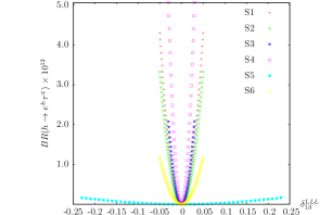
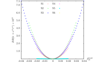
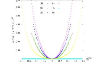
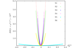
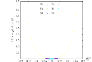
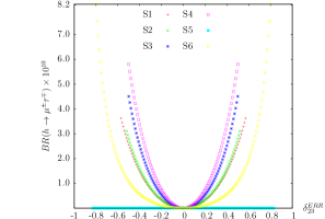
Figure 3: Lepton flavor violating decays $h\rightarrow e\tau$ and $h\rightarrow\mu\tau$ as a function of slepton mixing $\delta^{FAB}_{ij}$ for the six points defined in the Tab. 2.

5 Lepton Flavor Mixing Effects in the CMSSM-seesaw I 

After presenting the MI analysis in the previous section, here we investigate the predictions of the MSSM complemented with a ”see-saw´´ mechanism to explain neutrino masses. In this framework, values for $\delta^{FAB}_{ij}$ are radiatively generated even if the soft terms are assumed universal at the GUT scale.

One of the simpler implementations of the ”see-saw´´ mechanism on the MSSM is the type-I seesaw mechanism [7]. The superpotential for MSSM-Seesaw I can be written as

$$W = W_{\rm MSSM}+Y_{\nu}^{ij}\epsilon_{\alpha\beta}H_{2}^{\alpha}N_{i}^{c}L_{j}^{\beta}+\frac{1}{2}M_{N}^{ij}N_{i}^{c}N_{j}^{c},$$ (16)

where $W_{\rm MSSM}$ is given in Eq. (1) and $N_{i}^{c}$ is the additional superfield that contains the three right-handed neutrinos, $\nu_{Ri}$, and their scalar partners, $\tilde{\nu}_{Ri}$. $M_{N}^{ij}$ denotes the $3\times 3$ Majorana mass matrix for heavy right handed neutrino. The full set of soft SUSY-breaking terms is given by,

$$-{\cal L}_{\rm soft,SI} = -{\cal L}_{\rm soft}+(m_{\tilde{\nu}}^{2})^{i}_{j}{\tilde{\nu}}_{Ri}^{*}{\tilde{\nu}}_{R}^{j}+(\frac{1}{2}B_{\nu}^{ij}M_{N}^{ij}{\tilde{\nu}}_{Ri}^{*}{\tilde{\nu}}_{Rj}^{*}+A_{\nu}^{ij}h_{2}{\tilde{\nu}}_{Ri}^{*}{\tilde{l}}_{Lj}+{\rm h.c.})~{},$$ (17)

with ${\cal L}_{\rm soft}$ given by Eq. (2), $(m_{\tilde{\nu}}^{2})^{i}_{j}$, $A_{\nu}^{ij}$ and $B_{\nu}^{ij}$ are the new soft breaking parameters.

By the seesaw mechanism three of the neutral fields acquire heavy masses and decouple at high energy scale that we will denote as $M_{N}$, below this scale the effective theory contains the MSSM plus an operator that provides masses to the neutrinos.

$$W=W_{\rm MSSM}+\frac{1}{2}(Y_{\nu}LH_{2})^{T}M_{N}^{-1}(Y_{\nu}LH_{2}).$$ (18)

As right handed neutrinos decouple at their respective mass scales, at low energy we have the same particle content and mass matrices as in the MSSM. This framework naturally explains neutrino oscillations in agreement with experimental data [1]. At the electroweak scale an effective Majorana mass matrix for light neutrinos,

$$m_{\rm eff}=-\frac{1}{2}v_{u}^{2}Y_{\nu}\cdot M_{N}^{-1}\cdot Y^{T}_{\nu},$$ (19)

arises from Dirac neutrino Yukawa $Y_{\nu}$ (that can be assumed of the same order as the charged-lepton and quark Yukawas), and heavy Majorana masses $M_{N}$. The smallness of the neutrino masses implies that the scale $M_{N}$ is very high, ${\cal O}(10^{14}\,\,\mathrm{GeV})$.

From Eqs. (16) and (17) we can observe that one can choose a basis such that the Yukawa coupling matrix, $Y_{l}^{ij}$, and the mass matrix of the right-handed neutrinos, $M_{N}^{ij}$, are diagonalized as $Y_{l}^{\delta}$ and $M_{R}^{\delta}$, respectively. In this case the neutrino Yukawa couplings $Y_{\nu}^{ij}$ are not generally diagonal, giving rise to LFV  [73, 11, 13, 14, 74, 12] . Here it is important to note that the lepton-flavor conservation is not a consequence of the SM gauge symmetry, even in the absence of the right-handed neutrinos. Consequently, slepton mass terms can violate the lepton-flavor conservation in a manner consistent with the gauge symmetry. Thus the scale of LFV can be identified with the EW scale, much lower than the right-handed neutrino scale $M_{N}$. In the basis where the charged-lepton masses $Y_{\ell}$ is diagonal, the soft slepton-mass matrix acquires corrections that contain off-diagonal contributions from the RGE running from $M_{\rm GUT}$ down to the Majorana mass scale $M_{N}$, of the following form (in the leading-log approximation, assuming that $M_{N}$ is a common scale for the three heavy neutrino masses) [10]:

$$(m_{\tilde{L}}^{2})_{ij} \sim\frac{1}{16\pi^{2}}(6m^{2}_{0}+2A^{2}_{0})\left({Y_{\nu}}^{\dagger}Y_{\nu}\right)_{ij}\log\left(\frac{M_{\rm GUT}}{M_{N}}\right)\,$$

$$(m_{\tilde{e}}^{2})_{ij} \sim 0\,$$

$$(A_{l})_{ij} \sim\frac{3}{8\pi^{2}}{A_{0}Y_{l}}_{i}\left({Y_{\nu}}^{\dagger}Y_{\nu}\right)_{ij}\log\left(\frac{M_{\rm GUT}}{M_{N}}\right)\,$$ (20)

Below this scale, the off-diagonal contributions remain almost unchanged.

The values of $\delta^{FAB}_{ij}$ depend on the structure of $Y_{\nu}$ at a see-saw scale $M_{N}$ in a basis where $Y_{l}$ and $M_{N}$ are diagonal. By using the approach of Ref. [12] a general form of $Y_{\nu}$ containing all neutrino experimental information can be wtritten as:

$$Y_{\nu}=\frac{\sqrt{2}}{v_{u}}\sqrt{M_{R}^{\delta}}R\sqrt{m_{\nu}^{\delta}}U^{\dagger}~{},$$ (21)

where $R$ is a general orthogonal matrix and $m_{\nu}^{\delta}$ denotes the diagonalized neutrino mass matrix. In this basis the matrix $U$ can be identified with the $U_{\rm PMNS}$ matrix obtained as:

$$m_{\nu}^{\delta}=U^{T}m_{\rm eff}U~{}.$$ (22)

In order to find values for the slepton generation mixing parameters we need a specific form of the product $Y_{\nu}^{\dagger}Y_{\nu}$ as shown in Eq. (20). The simple consideration of direct hierarchical neutrinos with a common scale for right handed neutrinos provides a representative reference value. In this case using Eq. (21) we find

$$Y_{\nu}^{\dagger}Y_{\nu}=\frac{2}{v_{u}^{2}}M_{R}Um_{\nu}^{\delta}U^{\dagger}~{}.$$ (23)

Here $M_{R}$ is the common mass assigned to the $\nu_{R}$’s. In the conditions considered here, LFV effects are independent of the matrix $R$.

In order to perform our calculations, we used SPheno [75] to generate the CMSSM-seesaw I particle spectrum by running RGE from the GUT down to the EW scale. The particle spectrum was handed over in the form of an SLHA file [76] to FeynArts/FormCalc setup via FeynHiggs [60, 61, 62, 63, 64] to calculate LFVHD whereas cLFV decays were calculated with SPheno 3.2.4. The following section describes the details of our computational setup.

5.1 Input Parameters

For our scans of the CMSSM-seesaw I parameter space we use SPheno 3.2.4 [75] with the model “see-saw type-I” as in Ref. [43]. For the numerical analysis the values of the Yukawa couplings etc. have to be set to yield values in agreement with the experimental data for neutrino masses and mixings. In our computation, by considering a normal hierarchy among the neutrino masses, we fix $m_{\nu_{3}}\sim\sqrt{\Delta m^{2}_{\text{atm}}}\sim 0.05\,\,\mathrm{eV}$ and require $m_{\nu_{2}}/m_{\nu_{3}}=0.17$, $m_{\nu_{2}}\sim 100\cdot m_{\nu_{1}}$ consistent with the measured values of $\Delta m^{2}_{\text{sol}}$ and $\Delta m^{2}_{\text{atm}}$ [1]. The matrix $U$ in Eq. 21 is identified with $U_{\rm PMNS}$ with the ${\cal CP}$-phases set to zero and neutrino mixing angles set to the center of their experimental values. When the $Y_{\nu}$ of Eq. 21 is constructed using these values for $m_{\nu}^{\delta}$ and common values for $M_{R}^{\delta}=M_{N}$ we find representative values for the $\delta^{FAB}_{ij}$’s. Since these depend only on the product $Y_{\nu}^{\dagger}Y_{\nu}$, they are independent on the orthogonal matrix $R$ that can be set equal to the identity. By setting $M_{N}=10^{14}\,\,\mathrm{GeV}$, the values $Y_{\nu}$ remain perturbative. An example of models with almost degenerate $\nu_{R}$ can be found in [73]. For our numerical analysis we tested several scenarios and we found that the one defined here is the simplest and also the one with larger LFV prediction.

In order to get an overview about the size of the effects in the CMSSM-seesaw I parameter space, the relevant parameters $m_{0}$, $m_{1/2}$ have been scanned as, or in case of $A_{0}$ and $\tan\beta$ have been set to all combinations of

$$m_{0} \;=\;500\,\,\mathrm{GeV}\ldots 5000\,\,\mathrm{GeV}~{},$$ (24)

$$m_{1/2} \;=\;1000\,\,\mathrm{GeV}\ldots 3000\,\,\mathrm{GeV}~{},$$ (25)

$$A_{0} \;=\;-3000,-2000,-1000,0\,\,\mathrm{GeV}~{},$$ (26)

$$\tan\beta \;=\;10,20,35,45~{},$$ (27)

with $\mu>0$.

Our numerical results in the CMSSM-seesaw I are shown in Figs. 4 - 10. We have checked numerically that the dependence on $\tan\beta$ is not very prominent, but going from $A_{0}=0$ to $-3000\,\,\mathrm{GeV}$ has a strong impact on the $\delta^{FAB}_{ij}$. For small $A_{0}$ the size of the $\delta^{FAB}_{ij}$ is increasing with larger $m_{0}$ and $m_{1/2}$, for $A_{0}=-3000\,\,\mathrm{GeV}$ the largest values are found for small $m_{0}$ and $m_{1/2}$. We present the results in the $m_{0}$–$m_{1/2}$ plane for $\tan\beta=45$ and $A_{0}=-3000\,\,\mathrm{GeV}$ only, capturing the “largest” case. We start presenting the two most relevant $\delta^{FAB}_{ij}$. Left plot in Figs. 4 show $\delta^{LLL}_{13}$, right plot show $\delta^{LLL}_{23}$. As expected, $\delta^{LLL}_{23}$ turns out to be largest of ${\cal O}(0.01)$, while the $\delta^{LLL}_{13}$ is one order of magnitude smaller. Contraints imposed by the Higgs mass are displayed on the plots, the areas above the line corresponding to $M_{h}=128$ GeV and below $M_{h}=122$ GeV are excluded. Here we do not impose the satisfaction of the Cosmological bounds on neutralino relic density, because this is only achieved on a few selected areas of the plots (an updated review can be found in Ref.  [77] and references therein).

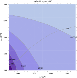
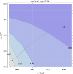
Figure 4: Contours of $\delta^{LLL}_{13}$ (Left) and $\delta^{LLL}_{23}$ (Right) in the $m_{0}$–$m_{1/2}$ plane in the CMSSM-seesaw I. The line labeled as 128, correponds to a prediction $M_{h}=128$ GeV (see text), on the area above this line the prediction for $M_{h}$ is higher.

5.2 ${\rm BR}(l_{i}\rightarrow l_{j}\gamma)$

The experimental limit BR($\mu\to e\gamma)<5.7\times 10^{-13}$ put severe constraints on slepton $\delta^{FAB}_{ij}$’s as discussed before. In Fig. 5, we show the predictions for BR($\mu\to e\gamma$) in $m_{0}$–$m_{1/2}$ plane for different values of $A_{0}$ and $\tan\beta$ in CMSSM-seesaw I. The selected values of $Y_{\nu}$ result in a large prediction for, e.g., BR($\mu\to e\gamma$) that can eliminate some of the $m_{0}$–$m_{1/2}$ parameter plane, in particular combinations of low values of $m_{0}$ and $m_{1/2}$. For $\tan\beta=10$ and $A_{0}=0$, BR($\mu\to e\gamma$) (upper left plot of Fig. 5) do not exclude any region in $m_{0}$–$m_{1/2}$ plane, whereas with $\tan\beta=10$ and $A_{0}=-3000$ lower left region below $m_{0},m_{1/2}=2000$ is excluded (see upper right plot of Fig. 5). For combinations like $\tan\beta=45,$ $A_{0}=0$ and $\tan\beta=45,$ $A_{0}=-3000$ even larger parts of the plane are excluded by BR($\mu\to e\gamma$). In Fig. 6 and Fig. 7, we show the predictions for BR($\tau\to e\gamma$) and BR($\tau\to\mu\gamma$) respectively. It can be seen that these processes do not reach their respective experimental bounds ${\rm BR}(\tau\rightarrow e\gamma)<3.3\times 10^{-8}$, ${\rm BR}(\tau\rightarrow\mu\gamma)<4.4\times 10^{-8}$. Consequently they do not exclude any parameter space.

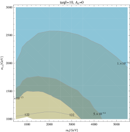
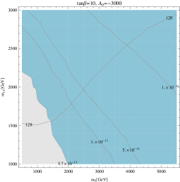
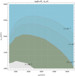
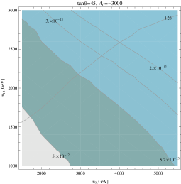
Figure 5: Contours of BR($\mu\to e\gamma$) in the $m_{0}$–$m_{1/2}$ plane for different values of $\tan\beta$ and $A_{0}$ in the CMSSM-seesaw I. The area below the $5.7\times 10^{-13}$ bound is excluded. The line labeled as 122 (128) on the plots of the left (right), correponds to a prediction $M_{h}=122(128)$ GeV (see text), for the area below (above) this line the prediction for $M_{h}$ is lower (higher) than this value.

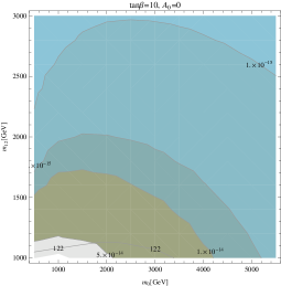
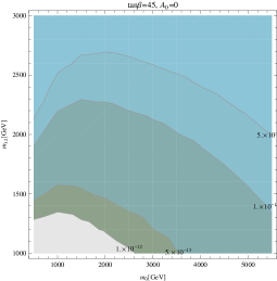
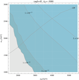
Figure 6: Contours of BR($\tau\to e\gamma$) in the $m_{0}$–$m_{1/2}$ plane for different values of $\tan\beta$ and $A_{0}$ in the CMSSM-seesaw I. Lines labeled as 122 and 128 are as descibred in Figs.4 and 5

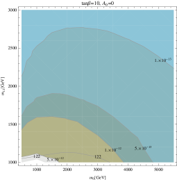
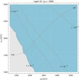
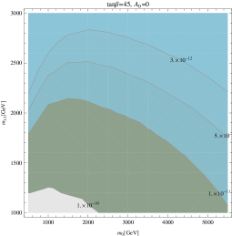
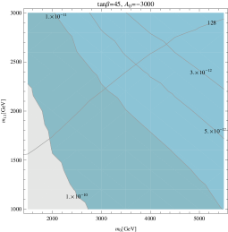
Figure 7: Contours of BR($\tau\to\mu\gamma$) in the $m_{0}$–$m_{1/2}$ plane for different values of $\tan\beta$ and $A_{0}$ in the CMSSM-seesaw I. Lines labeled as 122 and 128 are as descibred in Figs.4 and 5

5.3 ${\rm BR}(h\rightarrow l_{i}^{\pm}l_{j}^{\mp}$)

As we explained before, we do not expect large BR for LFVHD, due to the fact that in our models they are correlated to the restricitive bounds on the cLFV decays. Fig. 8 shows the results for BR($h\to e\mu$). The largest value is of the ${\cal O}(10^{-16})$ for low $m_{0}$ and $m_{1/2}$ values but is excluded from BR($\mu\to e\gamma$). In the allowed range they are typically ${\cal O}(10^{-18})$. Similarly Fig. 9 and Fig. 10 shows the predictions for BR($h\to e\tau$) and BR($h\to\tau\mu$) respectively. Predictions of the ${\cal O}(10^{-14})$ and ${\cal O}(10^{-12})$ are possible for BR($h\to e\tau$) and BR($h\to\tau\mu$) in the lower left region of the $m_{0}$–$m_{1/2}$ plane respectively but are excluded from BR($\mu\to e\gamma$) bound. In the allowed region they are of the ${\cal O}(10^{-16})$ or less. These results could not explain a CMS-type excess. We have also analysed other high scale see-saw models like Type II and Type III see-saw. However, the predictions for LFVHD are again very small compared to a possible CMS-type excess and we do not show them here. While it is possible to get large predictions for the LFVHD by using neutrino textures that somehow suppress BR($\mu\to e\gamma$), however for the realistic scenerios it is very difficult to get large predictions because off-diagonal enteries in the mass matrix of the slepton are the only source of LFV and large off-diagonal enteries will result in larger values of BR($\mu\to e\gamma$) unless mixing between first and second generation of the leptons is artificially suppressed. Although, ATLAS reports are not in contradiction with CMS ones, it remains to be seen how these results will develop with the LHC Run II.

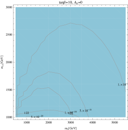
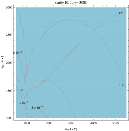
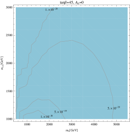
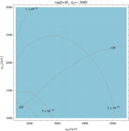
Figure 8: Contours of BR($h\to e\mu$) in the $m_{0}$–$m_{1/2}$ plane for different values of $\tan\beta$ and $A_{0}$ in the CMSSM-seesaw I. Lines labeled as 122 and 128 are as descibred in Figs.4 and 5

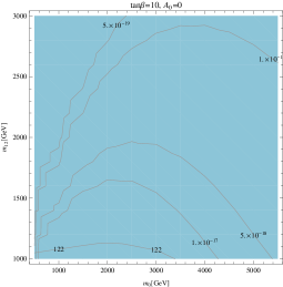
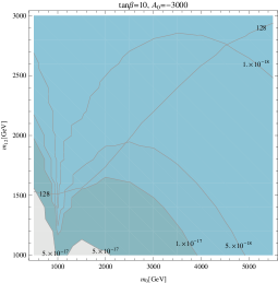
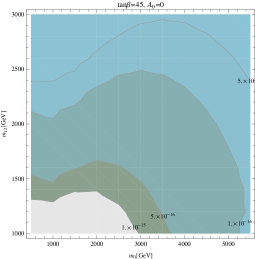
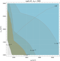
Figure 9: Contours of BR($h\to e\tau$) in the $m_{0}$–$m_{1/2}$ plane for different values of $\tan\beta$ and $A_{0}$ in the CMSSM-seesaw I. Lines labeled as 122 and 128 are as descibred in Figs.4 and 5

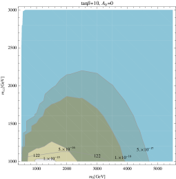
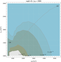
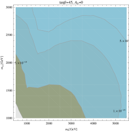
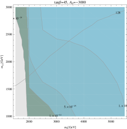
Figure 10: Contours of BR($h\to\tau\mu$) in the $m_{0}$–$m_{1/2}$ plane for different values of $\tan\beta$ and $A_{0}$ in the CMSSM-seesaw I. Lines labeled as 122 and 128 are as descibred in Figs.4 and 5

6 Conclusions

In this paper we have analyzed the Lepton Flavor Violation effects arising from the supersymmetric extension of the SM. We study several observables that can be sensitive to these effects. We take into account the restrictions imposed by the non-observation of charged Lepton Flavor Violation (cLFV) processes on the MSSM slepton mass parameters to study the impact of LFV effects to lepton flavour violating decays of ${\cal CP}$-even light Higgs boson (LFVHD). As a computation framework, we consider first a model independent selection of parameters of the MSSM and later some specific neutrino motivated SUSY models: constrained MSSM (CMSSM) extended by high scale seesaw models in particular Type-I seesaw mechanism.

For the model independent approach of Sect. 4 we consider six phenomenologically motivated benchmark points. These scenarios were studied before to extract the various $\delta^{FAB}_{ij}$ allowed by cLFV processes in Ref. [45]. Here, we impose their values to evaluate decay rates for the LFVHD. It turns out that it is very difficult to get large predictions for the LFVHD due to very strict constraints from cLFV decays. The prediction for ${\rm BR}(h\to\mu\tau)$ can be ${\cal O}(10^{-9})$ at maximum, which is very small compared to the possible CMS-type excess.

Going to the CMSSM-seesaw I  the numerical results were presented in Sect. 5. We have chosen a set of parameters consistent with the observed neutrino data and simultaneously induces large LFV effects and induces relatively large corrections to the calculated observables. Consequently, parts of the parameter space are excluded by the experimental bounds on ${\rm BR}(\mu\to e\gamma)$. As it was expected the prediction for the BR of LFVHD turned out very small in all the scenarios considered. We can conclude that we may need additional sources of lepton flavor violation (other then already present in the high scale see-saw models) to explain a CMS-type excess for the channel ${\rm BR}(h\to\mu\tau)$. Other neutrino motivated SUSY scenarios such as the inverse see-saw models can enhance lepton flavor violating Higgs boson decay rates [78, 79]. However, the latest results from CMS, if confirmed, will impose severe constraints on these models.

Acknowledgments

The work of S.H. and M.R. was partially supported by CICYT (grant FPA 2013-40715-P). M.G., S.H. and M.R. were supported by the Spanish MICINN’s Consolider-Ingenio 2010 Programme under grant MultiDark CSD2009-00064. M.E.G.  and M.R. acknowledges further support from the MICINN project FPA2014-53631-C2-2-P

References

- [1] S. Fukuda et al. [Super-Kamiokande Collaboration], Phys. Rev. Lett. 86, 5656 (2001). arXiv:hep-ex/0103033; S. Fukuda et al. [Super-Kamiokande Collaboration], Phys. Rev. Lett. 86, 5651 (2001). arXiv:hep-ex/0103032; S. Fukuda et al. [Super-Kamiokande Collaboration], Phys. Lett. B 539, 179 (2002). arXiv:hep-ex/0205075; M. Apollonio et al. [CHOOZ Collaboration], Phys. Lett. B 466, 415 (1999). arXiv:hep-ex/9907037; Q. Ahmad et al. [SNO Collaboration], Phys. Rev. Lett. 87, 071301 (2001). arXiv:nucl-ex/0106015; Q. Ahmad et al. [SNO Collaboration], Phys. Rev. Lett. 89, 011301 (2002). arXiv:nucl-ex/0204008; M. Ambrosio et al. [MACRO Collaboration], Phys. Lett. B 517, 59 (2001); G. Giacomelli and M. Giorgini [MACRO Collaboration], arXiv:hep-ex/0110021; K. Eguchi et al. [KamLAND Collaboration], arXiv:hep-ex/0212021
- [2] H. Nilles, Phys. Rept. 110, 1 (1984); H. Haber and G. Kane, Phys. Rept. 117, 75 (1985); R. Barbieri, Riv. Nuovo Cim. 11, 1 (1988)
- [3] L. J. Hall, V. A. Kostelecky and S. Raby, Nucl. Phys. B 267, 415 (1986).
- [4] F. Borzumati and A. Masiero, Phys. Rev. Lett. 57 (1986) 961;
- [5] V. Khachatryan et al. [CMS Collaboration], Phys. Lett. B 749 (2015) 337 arXiv:1502.07400 [hep-ex].
- [6] G. Aad et al. [ATLAS Collaboration], arXiv:1604.07730 [hep-ex].
- [7] P. Minkowski, Phys. Lett. B 67, 421 (1977); M. Gell-Mann, P. Ramond and R. Slansky, in Complex Spinors and Unified Theories eds. P. Van. Nieuwenhuizen and D. Freedman, Supergravity (North-Holland, Amsterdam, 1979), p.315 [Print-80-0576 (CERN)]; T. Yanagida, in Proceedings of the Workshop on the Unified Theory and the Baryon Number in the Universe, eds. O. Sawada and A. Sugamoto (KEK, Tsukuba, 1979), p.95; S. Glashow, in Quarks and Leptons, eds. M. Lévy et al. (Plenum Press, New York, 1980), p.687; R. Mohapatra and G. Senjanović, Phys. Rev. Lett. 44, 912 (1980)
- [8] S. F. King, Rept. Prog. Phys. 67 (2004) 107 hep-ph/0310204.
- [9] G. Senjanovic, Riv. Nuovo Cim. 34 (2011) 1. doi:10.1393/ncr/i2011-10061-8
- [10] J. Hisano, T. Moroi, K. Tobe and M. Yamaguchi, Phys. Rev. D 53 2442 (1996)
- [11] M. Gómez, G. Leontaris, S. Lola and J. Vergados, Phys. Rev. D 59, 116009 (1999). arXiv:hep-ph/9810291
- [12] J. Casas and A. Ibarra, Nucl. Phys. B 618, 171 (2001). arXiv:hep-ph/0103065
- [13] J. Ellis, M. E. Gómez, G. Leontaris, S. Lola and D. Nanopoulos, Eur. Phys. J. C 14, 319 (2000). arXiv:hep-ph/9911459
- [14] S. Antusch, E. Arganda, M. Herrero and A. Teixeira, JHEP 0611, 090 (2006). arXiv:hep-ph/0607263
- [15] S. Antusch, J. Kersten, M. Lindner, M. Ratz and M. A. Schmidt, JHEP 0503 (2005) 024.
- [16] J. Schwieger, T. S. Kosmas and A. Faessler, Phys. Lett. B 443 (1998) 7.
- [17] P. C. Divari, J. D. Vergados, T. S. Kosmas and L. D. Skouras, Nucl. Phys. A 703 (2002) 409 [nucl-th/0203066].
- [18] C. Biggio and L. Calibbi, JHEP 1010 (2010) 037 arXiv:1007.3750 [hep-ph].
- [19] A. J. R. Figueiredo and A. M. Teixeira, JHEP 1401 (2014) 015 arXiv:1309.7951 [hep-ph].
- [20] D. Chowdhury and K. M. Patel, Phys. Rev. D 87 (2013) no.9, 095018 arXiv:1304.7888 [hep-ph].
- [21] M. E. Krauss, W. Porod, F. Staub, A. Abada, A. Vicente and C. Weiland, Phys. Rev. D 90 (2014) no.1, 013008 arXiv:1312.5318 [hep-ph].
- [22] T. Goto, Y. Okada, T. Shindou, M. Tanaka and R. Watanabe, Phys. Rev. D 91 (2015) no.3, 033007 arXiv:1412.2530 [hep-ph].
- [23] J. Kersten, J. h. Park, D. Stöckinger and L. Velasco-Sevilla, JHEP 1408 (2014) 118 arXiv:1405.2972 [hep-ph].
- [24] A. Vicente, Adv. High Energy Phys. 2015 (2015) 686572 arXiv:1503.08622 [hep-ph].
- [25] R. Barbieri, L. J. Hall and A. Strumia, Nucl. Phys. B 445 (1995) 219 hep-ph/9501334.
- [26] M. E. Gomez and H. Goldberg, Phys. Rev. D 53 (1996) 5244 hep-ph/9510303.
- [27] M. E. Gomez, S. Lola, P. Naranjo and J. Rodriguez-Quintero, JHEP 1006 (2010) 053 arXiv:1003.4937 [hep-ph].
- [28] J. Ellis, K. Olive and L. Velasco-Sevilla, arXiv:1605.01398 [hep-ph].
- [29] Magg, M. and Wetterich, C. Phys. Lett. B94, 61 (1980).
- [30] Lazarides, G., Shafi, Q., and Wetterich, C. Nucl. Phys. B181, 287 (1981).
- [31] Foot, R., Lew, H., He, X. G., and Joshi, G. C. Z. Phys. C44, 441 (1989).
- [32] Ma, E. and Roy, D. P. Nucl. Phys. B644, 290–302 (2002).
- [33] A. Brignole and A. Rossi, Phys. Lett. B 566 (2003) 217 hep-ph/0304081.
- [34] A. Brignole and A. Rossi, Nucl. Phys. B 701 (2004) 3 hep-ph/0404211.
- [35] S. Kanemura, K. Matsuda, T. Ota, T. Shindou, E. Takasugi and K. Tsumura, Phys. Lett. B 599 (2004) 83 hep-ph/0406316.
- [36] P. Paradisi, JHEP 0602 (2006) 050 hep-ph/0508054.
- [37] M. Arana-Catania, E. Arganda and M. J. Herrero, JHEP 1309 (2013) 160 Erratum: [JHEP 1510 (2015) 192] arXiv:1304.3371 [hep-ph].
- [38] E. Arganda, M. J. Herrero, R. Morales and A. Szynkman, JHEP 1603 (2016) 055 arXiv:1510.04685 [hep-ph].
- [39] D. Aloni, Y. Nir and E. Stamou, JHEP 1604 (2016) 162 arXiv:1511.00979 [hep-ph].
- [40] J. Küblbeck, M. Böhm and A. Denner, Comput. Phys. Commun. 60, 165 (1990); T. Hahn, Comput. Phys. Commun. 140, 418 (2001). arXiv:hep-ph/0012260
- [41] T. Hahn and C. Schappacher, Comput. Phys. Commun. 143, 54 (2002). arXiv:hep-ph/0105349 The program and the user’s guide are available via www.feynarts.de .
- [42] M. Gómez, T. Hahn, S. Heinemeyer, M. Rehman, Phys. Rev. D 90, 074016 (2014). arXiv:1408.0663 [hep-ph]
- [43] M. E. Gomez, S. Heinemeyer and M. Rehman, Eur. Phys. J. C 75 (2015) no.9, 434 arXiv:1501.02258 [hep-ph].
- [44] E. Arganda, A. M. Curiel, M. J. Herrero and D. Temes, Phys. Rev. D 71 (2005) 035011 hep-ph/0407302.
- [45] M. Arana-Catania, S. Heinemeyer and M. Herrero, Phys. Rev. D 88, 015026 (2013). arXiv:1304.2783 [hep-ph]
- [46] Y. Kuno and Y. Okada, Rev. Mod. Phys. 73, 151 (2001). arXiv:hep-ph/9909265
- [47] S. Bilenky, S. Petcov and B. Pontecorvo, Phys. Lett. B 67, 309 (1977); W. Marciano and A. Sanda, Phys. Lett. B 67, 303 (1977)
- [48] T. Cheng, L.-F. Li, Phys. Rev. Lett. 45, 1908 (1980)
- [49] J. Adam et al. [MEG Collaboration], arXiv:1303.0754 [hep-ex].
- [50] B. Aubert et al. [BABAR Collaboration], Phys. Rev. Lett. 104, 021802 (2010) arXiv:0908.2381 [hep-ex].
- [51] U. Bellgardt et al. [SINDRUM Collaboration], Nucl. Phys. B 299, 1 (1988)
- [52] W. Bertl et al. [SINDRUM II Collaboration], Eur. Phys. J. C 47, 337 (2006).
- [53] K. Hayasaka, K. Inami, Y. Miyazaki, K. Arinstein, V. Aulchenko, T. Aushev, A. M. Bakich, A. Bay et al., Phys. Lett. B687 (2010) 139-143. arXiv:1001.3221 [hep-ex].
- [54] G. Aad et al. [ATLAS and CMS Collaborations], JHEP 1608 (2016) 045
- [55] D. de Florian et al. [LHC Higgs Cross Section Working Group Collaboration], “Handbook of LHC Higgs Cross Sections: 4. Deciphering the Nature of the Higgs Sector,” arXiv:1610.07922.
- [56] G. Aad et al. [ATLAS Collaboration], Phys. Rev. Lett. 112, 201802 (2014). arXiv:1402.3244 [hep-ex]
- [57] S. Chatrchyan et al. [CMS Collaboration], Eur. Phys. J. C 74, 2980 (2014). arXiv:1404.1344 [hep-ex]
- [58] http://cms-results.web.cern.ch/cms-results/public-results/preliminary-results/HIG-16-005/index.html
- [59] M. Gómez, S. Heinemeyer, M. Rehman, Phys. Rev. D 93, 095021 (2016). arXiv:1511.04342 [hep-ph]
- [60] S. Heinemeyer, W. Hollik and G. Weiglein, Comput. Phys. Commun. 124, 76 (2000). arXiv:hep-ph/9812320; T. Hahn, S. Heinemeyer, W. Hollik, H. Rzehak and G. Weiglein, Comput. Phys. Commun. 180, 1426 (2009) see www.feynhiggs.de
- [61] S. Heinemeyer, W. Hollik and G. Weiglein, Eur. Phys. J. C 9, 343 (1999). arXiv:hep-ph/9812472
- [62] G. Degrassi, S. Heinemeyer, W. Hollik, P. Slavich and G. Weiglein, Eur. Phys. J. C 28, 133 (2003). arXiv:hep-ph/0212020
- [63] M. Frank, T. Hahn, S. Heinemeyer, W. Hollik, R. Rzehak and G. Weiglein, JHEP 0702, 047 (2007). arXiv:hep-ph/0611326
- [64] T. Hahn, S. Heinemeyer, W. Hollik, H. Rzehak and G. Weiglein, Phys. Rev. Lett. 112, 141801 (2014). arXiv:1312.4937 [hep-ph]
- [65] H. Haber and Y. Nir, Nucl. Phys. B 335, 363 (1990)
-
[66]
S. Chatrchyan et al. [CMS Collaboration],
arXiv:1303.4571 [hep-ex];
Pedrame Bargassa, talk given at “Rencontres de Moriond EW 2014”,
https://indico.in2p3.fr/getFile.py/access?contribId=189&sessionId=0
&resId=1&materialId=slides&confId=9116;
Mike Flowerdew, talk given at “Rencontres de Moriond EW 2014”,
https://indico.in2p3.fr/getFile.py/access?contribId=169&sessionId=0
&resId=0&materialId=slides&confId=9116;
Paul Thompson, talk given at “Rencontres de Moriond EW 2014”,
https://indico.in2p3.fr/getFile.py/access?contribId=220&sessionId=8
&resId=0&materialId=slides&confId=9116;
Kevin Einsweiler, talk given at “Rencontres de Moriond EW 2014”,
https://indico.in2p3.fr/getFile.py/access?contribId=227&sessionId=1
&resId=1&materialId=slides&confId=9116 . - [67] P. Bechtle, O. Brein, S. Heinemeyer, G. Weiglein and K. Williams, Comput. Phys. Commun. 181, 138 (2010). arXiv:0811.4169 [hep-ph]; Comput. Phys. Commun. 182, 2605 (2011). arXiv:1102.1898 [hep-ph]; P. Bechtle, O. Brein, S. Heinemeyer, O. Stål, T. Stefaniak, G. Weiglein and K. Williams, Eur. Phys. J. C 74, 2693 (2014). arXiv:1311.0055 [hep-ph]
- [68] K. S. Babu and C. Kolda, Phys. Rev. Lett. 89 (2002) 241802 hep-ph/0206310.
- [69] A. Dedes, J. R. Ellis and M. Raidal, Phys. Lett. B 549 (2002) 159 hep-ph/0209207.
- [70] M. Cannoni and O. Panella, Phys. Rev. D 79 (2009) 056001 arXiv:0812.2875 [hep-ph].
- [71] J. Hisano, S. Sugiyama, M. Yamanaka and M. J. S. Yang, Phys. Lett. B 694 (2011) 380 arXiv:1005.3648 [hep-ph]. [58]
-
[72]
The ATLAS Collaboration, ATLAS-CONF-2016-085.
The CMS Collaboration, CMS-PAS-HIG-16-037. - [73] M. Cannoni, J. Ellis, M. Gómez and S. Lola, Phys. Rev. D 88, 075005 (2013). arXiv:1301.6002 [hep-ph]
- [74] J. Ellis, M. Gómez and S. Lola, JHEP 0707, 052 (2007). arXiv:hep-ph/0612292
- [75] W. Porod, Comput. Phys. Commun. 153, 275 (2003). arXiv:hep-ph/0301101
- [76] P. Skands et al., JHEP 0407, 036 (2004). arXiv:hep-ph/0311123; B. Allanach et al., Comput. Phys. Commun. 180, 8 (2009). arXiv:0801.0045 [hep-ph]
- [77] K. A. Olive, PoS DSU 2015 (2016) 035 arXiv:1604.07336 [hep-ph].
- [78] E. Arganda, M. J. Herrero, X. Marcano and C. Weiland, Phys. Rev. D 93 (2016) no.5, 055010 arXiv:1508.04623 [hep-ph].
- [79] A. Hammad, S. Khalil and C. S. Un, arXiv:1605.07567 [hep-ph].