New numerical approaches for modeling thermochemical convection in a compositionally stratified fluid

Abstract

Seismic imaging of the mantle has revealed large and small scale heterogeneities in the lower mantle; specifically structures known as large low shear velocity provinces (LLSVP) below Africa and the South Pacific. Most interpretations propose that the heterogeneities are compositional in nature, differing in composition from the overlying mantle, an interpretation that would be consistent with chemical geodynamic models. The LLSVP’s are thought to be very old, meaning they have persisted throughout much of Earth’s history. Numerical modeling of persistent compositional interfaces presents challenges, even to state-of-the-art numerical methodology. For example, some numerical algorithms for advecting the compositional interface cannot maintain a sharp compositional boundary as the fluid migrates and distorts with time dependent fingering due to the numerical diffusion that has been added in order to maintain the upper and lower bounds on the composition variable and the stability of the advection method. In this work we present two new algorithms for maintaining a sharper computational boundary than the advection methods that are currently openly available to the computational mantle convection community; namely, a Discontinuous Galerkin method with a Bound Preserving limiter (DGBP) and a Volume-of-Fluid (VOF) interface tracking algorithm. We compare these two new methods with two approaches commonly used for modeling the advection of two distinct, thermally driven, compositional fields in mantle convection problems; namely, an approach based on a high-order accurate finite element method (FEM) advection algorithm that employs an artificial viscosity technique known as ‘Entropy Viscosity’ (FEM-EV) to maintain the upper and lower bounds on the composition variable as well as the stability of the advection algorithm and the advection of particles that carry a scalar quantity representing the location of each compositional field. All four of these algorithms are implemented in the open source FEM code ASPECT, which we use to compute the velocity, pressure, and temperature fields associated with the underlying flow field. We compare the performance of these four algorithms by computing the solution to an initially compositionally stratified fluid that is subject to a thermal gradient at a Rayleigh number of $\mathrm{Ra}=10^{5}$ with a buoyancy ratio of $\mathrm{B}=1.0$. For $\mathrm{B}=1.0$, a value for which the initial stratification of the compositional fields persists indefinitely, our computations demonstrate that the entropy viscosity-based method has far too much numerical diffusion to yield meaningful results. On the other hand, the DGBP method yields good results, although small amounts of each compositional field are numerically entrained within the other compositional field. The particle method yields yet better results than this, but some particles representing the denser fluid are entrained in the upper, less dense fluid and are advected to the top of the computational domain and, similarly, particles representing the less dense fluid are entrained in the lower, denser fluid and are advected to the bottom of the computational domain. The VOF method maintains a sharp interface between the two compositions on a subgrid scale throughout the computation. We also compute the same problem with $\mathrm{Ra}=10^{5}$ for a range of buoyancy ratios $\mathrm{B}\,=\,0.0,\,0.1,\,0.2,\,\ldots,\,1.0$ using the DGBP method in order to demonstrate the utility of this method when the stratified layer overturns and kinematic mixing begins. In this regime the VOF algorithm is not suitable for modeling the interface between the two compositional fields, since this would require that the grid size $h\to 0$ as the curvature $\sigma$ of the interface between the two compositional fields goes to infinity, $\sigma\to\infty$.

Keywords: Thermal Convection, Stratified Fluid, Composition Advection, Finite Element Method, Entropy Viscosity, Discontinuous Galerkin Method, Particle Method, Volume-of-Fluid, Stokes Equations, Bound Preserving Limiter

1 Introduction

A major unresolved question in geodynamics is whether mantle convection consists of a single layer or two separate layers. Seismic studies have shown deep penetration of subducted lithosphere which favors whole mantle convection. However isotopic studies provide strong evidence for a well mixed upper mantle but a lower mantle reservoir containing primordial material and unmixed subducted material. The near uniform isotopic ratios of most mid-ocean ridge basalts indicate that this volcanism is sampling a near homogeneous upper-mantle reservoir. However, the extreme isotopic heterogeneities of ocean island basalts indicate that there is a deep source. This source includes primordial materials as well as a variety of subducted materials that have not been mixed into the mantle. The transport of mantle from the deep source is attributed to mantle plumes [22, 47].

Recent studies utilizing seismic imaging have revealed large regions with anomalous seismic properties in the lower mantle. There are two dome like regions beneath Africa and the Pacific with low shear-wave velocities extending some 1000 km above the core-mantle boundary with horizontal dimensions of several thousand kilometers. These are known as large low shear-velocity provinces (LLSVPs). Most interpretations propose that the heterogeneities are compositional in nature, differing from the overlying mantle, an interpretation that would be consistent with chemical geodynamic models. The LLSVP’s are thought to be very old, meaning they have persisted throughout much of Earth’s history [2, 6, 10].

Mantle convection with compositional differences, together with a thermal contribution, is known as thermal-chemical convection. [41] has given a comprehensive review of the influence of compositional buoyancy on mantle convection both in terms of evidence for buoyancy structures in the mantle and models of the influence of compositional buoyancy on thermal-chemical convection. Thermal-chemical convection with applications to the mantle requires distinct regions with different compositions and densities. Molecular diffusion that can mix regions with different compositions can occur only on very small scales in the mantle on geological time scales, centimeters to meters. Thus, mixing is predominantly kinematic with sharp compositional interfaces [21].

Numerical modeling of persistent compositional interfaces presents challenges, even to state-of-the-art numerical methodology. Currently, in the computational mantle convection community many numerical algorithms for modeling distinct compositional regions do not maintain sharp boundaries between distinct compositions as they migrate and distort with time dependent fingering. In particular, some of these algorithms exhibit compositional diffusion, either as an unwanted numerical artifact of the algorithm or artificial diffusion, which is an explicit design feature of the algorithm, or both. Artificial diffusion, which is typically referred to as artificial viscosity, is a quantity that is added to the (numerical) advection equation in order to maintain the upper and lower bounds on the value of the compositional variable and also, for Finite Element Methods (FEM), to maintain the stability of the advection algorithm [48], [13]. This numerical technique is described in more detail in Section 3.4.1. Note that we prefer to use the term artificial diffusion instead of artificial viscosity. Numerical algorithms that allow the compositional boundary to diffuse, whether as a numerical artifact or as an intentional part of the advection method are inherently in conflict with the fact that the true sharp compositional boundary must persist indefinitely.

A number of studies of the role of compositional discontinuities on mantle convection have been carried out. Numerical studies include [29], [26], [43], and [11]. [7] has carried out an extensive laboratory studies.

In this paper we exam four alternative algorithms for numerically modeling this compositional discontinuity. All of these algorithms are implemented as part of the open source mantle convection software ASPECT, which is described in detail in [23]. Each algorithm is designed to model the motion of two distinct compositional regions. These four algorithms are: 1) the compositional advection method with so-called ‘Entropy Viscosity’ (FEM-EV), which was the first advection method to be implemented in ASPECT, 2) a new Discontinuous Galerkin Bound Preserving (DGBP) compositional advection method, 3) Volume-of-Fluid (VOF) interface tracking, and 4) Particles. These algorithms will be described in detail in Sections 3.4.1–3.4.4 and their relative performance will be examined and discussed in Section 4 below.

Table 1: A list of symbols used in this paper.

Symbol	Quantity	Unit	Symbol	Quantity	Unit
$\bf{u}$	Velocity	$m/s$	$\rho$	Density	$kg\cdot m^{-3}$
$p$	Dynamic pressure	Pa	$\Delta\rho$	Density difference	$kg\cdot m^{-3}$
$T_{0}$	Temperature at the top	K	$D$	Compositional diffusivity	$m^{2}/s$
$T_{1}$	Temperature at the bottom	K	$\alpha$	Thermal expansion coefficient	1/K
$T$	Temperature	K	$d$	Vertical thickness of fluid layer	m
$\Delta T$	Temperature difference	K	$Pr$	Prandtl number	$\frac{\mu}{\rho\kappa}$
$C$	Composition	-	$Le$	Lewis number	$\frac{\kappa}{D}$
$\mu$	Viscosity	Pa $\cdot$ s	$Ra$	Rayleigh number	$\frac{\rho_{0}{\bf{g}}\alpha\Delta Td^{3}}{\mu\kappa}$
$\kappa$	Thermal diffusivity	$m^{2}/s$	$B$	Buoyancy ratio	$\frac{\Delta\rho}{\rho_{0}\alpha\Delta T}$
$\rho_{0}$	Reference density	$kg\cdot m^{-3}$

2 The Model Problem

2.1 The Dimensional Form of the Equations

In order to study alternative numerical algorithms for modeling persistent compositional interfaces we will consider a problem that emphasizes the effect of a compositional density difference on thermal convection. We consider a two-dimensional flow in a horizontal fluid layer with a thickness $d$. In dimensional terms our problem domain $\Omega$ has width $3d$ and depth $d$. At a given reference temperature $T_{0}$ the region $0\leq y<d/2$ has a compositional density of $\rho_{0}$ and the region $d/2<y\leq d$ has a compositional density of $\rho_{0}+\Delta\rho$ where $\Delta\rho\,\ll\,\rho_{0}$.

We also introduce a composition variable $C(x,y,t)$ defined by

$$C=\frac{\rho-\rho_{0}}{\Delta\rho}\,.$$ (1)

The composition $C$ is the concentration of the dense fluid as a function of space and time. The initial condition for $C$ is

$$C(x,y,t=0)\,=\,\left\{\begin{array}[]{ll}0&\text{for}\quad 0\leq y\leq d/2\,,\\ 1&\text{for}\quad d/2<y\leq d\,.\end{array}\right.$$ (2)

The upper boundary, at $y=0$, has temperature $T_{0}$ and the lower boundary at $y=d$ has temperature $T_{1}$. The fluid is assumed to have a constant viscosity $\mu$ which is large. The Prandtl number

$$Pr\,=\,\frac{\mu}{\rho_{0}\kappa}\,\gg\,1\,,$$ (3)

where $\kappa$ is the thermal diffusivity so that inertial effects can be neglected. The fluids in the high density and low density layers are immiscible; i.e., they cannot mix by diffusion. The Lewis number

$$Le\,=\,\frac{\kappa}{D}\,\gg\,1\,,$$ (4)

where $D$ is the diffusion coefficient for the compositional variable $C$ (Table 1). Thus, the discontinuous boundary between the high density and low density fluids is preserved indefinitely.

The problem we have posed requires the solution of the standard equations for thermal convection with the addition of an equation for the compositional field $C$ that ’tracks’ the compositional density. We make the assumption that the Boussinesq approximation holds; namely, that density differences associated with convection $\rho_{0}\alpha(T_{1}-T_{0})$ and $\Delta\rho$ are small compared with the reference density $\rho_{0}$.

$$\rho(x,y,t)\,=\,\rho_{0}\,(1-\alpha(T-T_{0}))\,+\,\Delta\rho\,C\,.$$ (5)

The governing equations have been discussed in detail by [38] (Chapter 6). Conservation of mass requires

$$\frac{\partial u}{\partial x}+\frac{\partial v}{\partial y}=0$$ (6)

where $x$ and $y$ denote the horizontal and vertical spacial coordinates, oriented as shown in Figure 1, and $u$ and $v$ denote the horizontal and vertical velocity components, respectively. We use the Stokes equations

$$0 =\frac{-\partial P}{\partial x}+\mu(\frac{\partial^{2}u}{\partial x^{2}}+\frac{\partial^{2}u}{\partial y^{2}})\,,$$ (7)

$$0 =\frac{-\partial P}{\partial y}+\mu(\frac{\partial^{2}v}{\partial x^{2}}+\frac{\partial^{2}v}{\partial y^{2}})-\rho_{0}\alpha(T-T_{0})g+\Delta\rho Cg\,,$$ (8)

where $P$ is the dynamic pressure, $\alpha$ is the coefficient of thermal expansion, and $g$ is the gravitational acceleration in the positive (downward) $y$ direction as shown in Figure 1. Conservation of energy requires

$$\frac{\partial T}{\partial t}+u\frac{\partial T}{\partial x}+v\frac{\partial T}{\partial y}=\kappa(\frac{\partial^{2}T}{\partial x^{2}}+\frac{\partial^{2}T}{\partial y^{2}})\,.$$ (9)

With no diffusion, i.e., $D=0$, the composition variable $C$ satisfies the advection equation

$$\frac{\partial C}{\partial t}+u\frac{\partial C}{\partial x}+v\frac{\partial C}{\partial y}=0\,.$$ (10)

2.2 The Nondimensional Form of the Equations

We introduce the non-dimensional variables

$$x^{\prime} =\frac{x}{d}, y^{\prime} =\frac{y}{d}, t^{\prime} =\frac{\kappa}{d^{2}}\,t,$$ (11)

$$u^{\prime} =\frac{d}{\kappa}\,u, v^{\prime} =\frac{d}{\kappa}\,v, \rho^{\prime} =\frac{\rho}{\rho_{0}},$$

$$T^{\prime} =\frac{T-T_{0}}{T_{1}-T_{0}}, P^{\prime} =\frac{d^{\,2}P}{\mu\kappa},$$

and the two nondimensional parameters, the Rayleigh number $Ra$ and the buoyancy ratio $B$

$$Ra=\frac{\rho_{0}\,g\,\alpha(T_{1}-T_{0})d^{3}}{\mu\,\kappa},$$ (12)

$$B\,=\,\frac{\Delta\rho}{\rho_{0}\alpha(T_{1}-T_{0})}.$$ (13)

Substitution of equations (11)–(13) into equations (6)–(10) gives

$$\frac{\partial u^{\prime}}{\partial x^{\prime}}+\frac{\partial v^{\prime}}{\partial y^{\prime}} =0\,,$$ (14)

$$0 =\frac{-\partial P^{\prime}}{\partial x^{\prime}}+\frac{\partial^{2}u^{\prime}}{\partial x^{{}^{\prime}2}}+\frac{\partial^{2}u^{\prime}}{\partial y^{{}^{\prime}2}}\,,$$ (15)

$$0 =\frac{-\partial P^{\prime}}{\partial y^{\prime}}+\frac{\partial^{2}v^{\prime}}{\partial x^{{}^{\prime}2}}+\frac{\partial^{2}v^{\prime}}{\partial y^{{}^{\prime}2}}-\mathrm{Ra}T^{\prime}+\mathrm{Ra}\mathrm{B}C\,,$$ (16)

$$\frac{\partial T^{\prime}}{\partial t^{\prime}}+u^{\prime}\frac{\partial T^{\prime}}{\partial x^{\prime}}+v^{\prime}\frac{\partial T^{\prime}}{\partial y^{\prime}} =\frac{\partial^{2}T^{\prime}}{\partial x^{{}^{\prime}2}}+\frac{\partial^{2}T^{\prime}}{\partial y^{{}^{\prime}2}}\,,$$ (17)

$$\frac{\partial C}{\partial t^{\prime}}+u^{\prime}\frac{\partial C}{\partial x^{\prime}}+v^{\prime}\frac{\partial C}{\partial y^{\prime}} =0\,.$$ (18)

Figure 1: The geometry of the (nondimensional) computational domain $\Omega$ shown with the temperature boundary conditions on the four side walls. The velocity boundary conditions on the side walls are $\mathbf{u}\cdot\mathbf{n}=0$ (no flow) and $\partial\bf{u}/\partial\boldsymbol{\tau}=0$ (free slip) where $\mathbf{n}$ and $\boldsymbol{\tau}$ are the unit normal and tangential vectors to the boundary respectively.

This is the superposition of a Rayleigh-Taylor problem and a Rayleigh-Bernard problem. In the isothermal limit ($T_{0}=T_{1}$) it is the classic Rayleigh-Taylor problem ([47], pp. 285-286). If $C$ is positive, a light fluid is above the heavy fluid and in a downward gravity field the fluid layer is stable. If $\Delta\rho$ is negative, a heavy fluid lies over a light fluid and the layer is unstable. Flows will transfer the heavy fluid to the lower half and the light fluid to the upper half. The density layer will overturn. If $\Delta\rho=0$ this is the classic Rayleigh-Bernard problem for thermal convection. The governing parameter is the Rayleigh number. If $0<Ra<Ra_{c}$, the critical Rayleigh number, no flow will occur. If $Ra_{c}<Ra<Ra_{t}$ steady cellular flow will occur. If $Ra>Ra_{t}$ the flow becomes unsteady and thermal turbulence develops.

If $Ra>Ra_{c}$ and $B$ is small, the boundary between the density differences will not block the flow driven by thermal convection. Kinematic mixing will occur and the composition will homogenize so that the density is constant and $C=\frac{1}{2}$. Whole layer convection will occur. If B is large, the density difference boundary will block the flow driven by thermal convection. The compositional boundary will be displaced vertically but will remain intact. Layered convection will occur with the compositional boundary, the boundary between the convecting layers. The Rayleigh number defined in equation (12) is based on the domain thickness $d$. This is the case for which we will show numerical computations.

3 The Numerical Methodology

In the following discussion of the numerical methodology, we will only consider the dimensionless equations (14)-(18) and drop the primes associated with the dimensionless variables. The vector form of the dimensionless equations on the 2D rectangular domain $\Omega=[0,3]\times[0,1]$ shown in Figure 1 are given by

$$-\nabla^{2}{\bf{u}}+\nabla P =(-RaT+RaBC)\,{\bf{g}}$$ (19)

$$\nabla\cdot{\bf{u}} =0,$$ (20)

$$\frac{\partial T}{\partial t}+{\bf u}\cdot\nabla T =\nabla^{2}T,$$ (21)

$$\frac{\partial C}{\partial t}+{\bf u}\cdot\nabla C =0,$$ (22)

where ${\bf u}=(u,v)$, and ${\bf g}=(0,1)$ is the unit vector pointing downward. We also assume no-flow and free-slip velocity boundary conditions on all boundaries,

$$\mathbf{u}\cdot\mathbf{n} =0\qquad\text{(no-flow)}\,,$$ (23)

$$\frac{\partial\bf{u}}{\partial\boldsymbol{\tau}} =0\qquad\text{(free slip)}\,,$$ (24)

where $\mathbf{n}$ and $\boldsymbol{\tau}$ are the unit normal and tangential vectors to the boundary respectively. We impose Dirichlet boundary conditions for the temperature on the top and bottom of the computational domain and Neumann boundary conditions (no heat flux) on the sides of the computational domain,

$$T(x,0,t)=0\,,$$ (25)

$$T(x,1,t)=1\,,$$ (26)

$$\partial_{x}T(0,y,t)=0\,,$$ (27)

$$\partial_{x}T(0,y,t)=0\,.$$ (28)

The geometry of the computational domain together with the boundary conditions on the temperature are shown in Figure 1.

3.1 Decoupling of the Nonlinear System

The incompressible Stokes equations can be considered as a constraint on the temperature and composition at any given time leading to a highly nonlinear system of equations. To solve this nonlinear system, we apply the Implicit Pressure Explicit Saturation (IMPES) approach, which was originally developed for computing approximations to solutions of equations for modeling problems in porous media flow [39, 20], to decouple the incompressible Stokes equations (19) –(20) from the temperature and compositional equations (21)–(22). This leads to three discrete systems of linear equations, the Stokes equations, the temperature equation and the composition equation, thereby allowing them to be solved easily and efficiently.

3.2 Discretization of the Stokes Equations

Let $t_{k}$ denote the discretized time at the kth time step with a time step size $\Delta t_{k}=t_{k}-t_{k-1}$, $k=0,\,1,\,\ldots$ Given the temperature $T^{k}$ and composition $C^{k}$ at time $t=t_{k}$, we first solve for our approximation to the Stokes equations (19) –(20) to obtain the velocity $\mathbf{u}^{k}=(u^{k},\,v^{k})$ and pressure $P^{k}$

$$-\nabla^{2}{\bf{u}}^{k}+\nabla P^{k} =(-RaT^{k}+RaBC^{k}){\bf{g}},$$ (29)

$$\nabla\cdot{\bf{u}}^{k} =0.$$ (30)

For the incompressible Stokes equations (29)-(30), we use the standard mixed FEM method with a Taylor-Hood element [8] for the spatial approximation of the incompressible Stokes equations (19)–(20). If we assume the finite element space is $(X(\Omega))^{n}\times Y(\Omega)$, where $n$ denotes the spacial dimension then the problem is to find $({\bf u}^{k},P^{k})\in(X(\Omega))^{n}\times Y(\Omega)\cap(H^{1}_{0}(\Omega))^{n}\times L_{2}(\Omega)$ such that

$$\int\limits_{\Omega}\nabla{\bf{u}}^{k}\cdot\nabla{\bf{\Phi}}dxdy-\int\limits_{\Omega}P^{k}\nabla\cdot{\bf{\Phi}}dxdy =\int\limits_{\Omega}(-RaT^{k}+RaBC^{k}){\bf g}\cdot{\bf\Phi}dxdy,$$ (31)

$$\int\limits_{\Omega}\nabla\cdot{\bf{u}}^{k}\,q\,dx\,dy =0$$ (32)

for any $({\bf\Phi},q)\in(X(\Omega))^{n}\times Y(\Omega)\cap(H^{1}_{0}(\Omega))^{n}\times L_{2}(\Omega)$. If we introduce the inner product of two vector functions $\mathbf{u}$ and $\mathbf{v}$ on a given domain $\Omega$

$$(\mathbf{u},\mathbf{v})_{\Omega}=\int\limits_{\Omega}{\bf{u}}\cdot{\bf{v}}dxdy,$$ (33)

and the inner product of two scalar functions $u$ and $v$ on $\Omega$

$$(u,v)_{\Omega}=\int\limits_{\Omega}\,u\,v\,dx\,dy$$ (34)

then we can rewrite the equations (31)–(32) as

$$(\nabla{\bf{u}}^{k},\nabla{\bf{\Phi}})_{\Omega}-(P^{k},\nabla\cdot{\bf{\Phi}})_{\Omega} =(Ra(B\ C^{k}-T^{k}){\bf g},{\bf\Phi})_{\Omega},$$ (35)

$$(\nabla\cdot{\bf{u}}^{k},q)_{\Omega} =0\,.$$ (36)

3.3 Discretization of the Temperature Equation

In all of the computations presented here we use the algorithm currently implemented in ASPECT to approximate the spatial and temporal terms in the temperature equation (21). This algorithm includes the entropy viscosity stabilization technique described in [14] and [23]. The weak form of this spatial discretization is

$$(\frac{\partial T}{\partial t},\psi)_{\Omega}+({\bf u}\cdot\nabla T,\psi)_{\Omega} =-(\nabla T,\nabla\psi)_{\Omega}-(\nu_{h}(T)\nabla T,\nabla\psi)_{\Omega}+(\frac{\partial T}{\partial{\bf n}},\psi)_{\Gamma_{D}}$$ (37)

where $\nu_{h}(T)$ is the entropy viscosity function as defined in [23], except here we do not use a second-order extrapolation to treat the advection term $({\bf u}\cdot\nabla T,\psi)$ and the entropy viscosity term $(\nu_{h}(T)\nabla T,\nabla\psi)_{\Omega}$ explicitly. The entropy-viscosity function $\nu_{h}^{k}(T)$ is a non-negative constant within each cell that only adds artificial diffusion in cells for which the local Péclet number $\mathrm{Pe}=\mathrm{Ra}\ \mathrm{Pr}$ is large and the solution is not smooth. We use the fully implicit adaptive Backward Differentiation Formula of order 2 (BDF2) [49, 23] to discretize the temperature equation in time. Thus, the full discretization of the temperature equation is

$$(\frac{1}{\Delta t_{k+1}}\left(\frac{2\Delta t_{k+1}+\Delta t_{k}}{\Delta t_{k+1}+\Delta t_{k}}T^{k+1}-\frac{\Delta t_{k+1}+\Delta t_{k}}{\Delta t_{k}}T^{k}+\frac{\Delta t_{k+1}^{2}}{\Delta t_{k}(\Delta t_{k+1}+\Delta t_{k})}T^{k-1}\right),\psi)_{\Omega}$$

$$= -({\bf u}^{k}\cdot\nabla T^{k+1},\psi)_{\Omega}-(\nabla T^{k+1},\nabla\psi)_{\Omega}-(\nu_{h}^{k}(T)\nabla T^{k+1},\nabla\psi)_{\Omega}+(\frac{\partial T^{k+1}}{\partial{\bf n}},\psi)_{\Gamma_{D}}\,.$$ (38)

3.4 Discretization of the Composition Equation

We use one of the four algorithms described below to discretize the composition equation (22).

3.4.1 The Finite Element Advection Algorithm with Entropy Viscosity

This is the first advection algorithm that was implemented in ASPECT. It is based on the same spatial discretization as shown in equation (37). However, the entropy-viscosity stabilization term on the right-hand side in

$$(\frac{\partial C}{\partial t},\psi)_{\Omega}+({\bf u}\cdot\nabla C,\psi)_{\Omega}\,=\,-(\nu_{h}^{k}(C)\nabla C,\nabla\psi)_{\Omega}$$ (39)

is computed separately for the composition field; i.e, it does not have the same value in each cell as does the entropy-viscosity $\nu_{h}^{k}(T)$ for the temperature field. In equation (39) the entropy function $\nu_{h}^{k}(C)$ has the same purpose as $\nu_{h}^{k}(T)$ and is defined by

$$\nu^{e}_{h}=\frac{\alpha\,h^{2}\,R(\,r_{e}(C_{h}))}{\|E(C_{h})-\bar{E}\|_{\infty,\Omega}}\,.$$ (40)

See [14],[23] for details. We also use the adaptive BDF2 algorithm for the time discretization, leading to the following FEM Entropy Viscosity (FEM-EV) discretization of equation (22),

$$(\frac{1}{\Delta t_{k+1}} \left(\frac{2\Delta t_{k+1}+\Delta t_{k}}{\Delta t_{k+1}+\Delta t_{k}}C^{k+1}-\frac{\Delta t_{k+1}+\Delta t_{k}}{\Delta t_{k}}C^{k}+\frac{\Delta t_{k+1}^{2}}{\Delta t_{k}(\Delta t_{k+1}+\Delta t_{k})}C^{k-1}\right),\psi)_{\Omega}$$

$$= -({\bf u}^{k}\cdot\nabla C^{k+1},\psi)_{\Omega}-(\nu_{h}^{k}(C)\nabla C^{k+1},\nabla\psi)_{\Omega}\,.$$ (41)

3.4.2 The Discontinuous Galerkin Bound Preserving Advection Algorithm

In this algorithm we use adaptive BDF2 to discretize the advection equation (22) for the composition in time as shown in equation (3.4.1). However we use a Discontinuous Galerkin method with a Bound Preserving limiter (DGBP) for the discretization of the spatial terms in equation (22). The DG method differs from the classic continuous Galerkin FEM, since it allows for discontinuities between elements [37, 40]. If we denote the discretized computational domain by $\Omega=\cup_{e=1}^{E}\Omega^{e}$, where $\Omega^{e}$ denotes non-overlapping body-conforming quadrilateral elements, and let $V_{N}(\Omega)$ denote the DG element space, then fully discretized problem is as follows. Find $C^{k+1}\in V_{N}(\Omega)$ such that

$$(\frac{1}{\Delta t_{k+1}}\left(\frac{2\Delta t_{k+1}+\Delta t_{k}}{\Delta t_{k+1}+\Delta t_{k}}C^{k+1}-\frac{\Delta t_{k+1}+\Delta t_{k}}{\Delta t_{k}}C^{k}+\frac{\Delta t_{k+1}^{2}}{\Delta t_{k}(\Delta t_{k+1}+\Delta t_{k})}C^{k-1}\right),\psi)_{\Omega_{e}}$$

$$= -({\bf u}^{k}\cdot\nabla C^{k+1},w)_{\Omega_{e}}+({\bf u}^{k}\cdot{\bf n}C^{k+1},w)_{\partial\Omega_{e}}-({\bf u}^{k}\cdot{\bf n}C^{k+1,*},w)_{\partial\Omega_{e}}$$ (42)

for any $w\in V_{N}$. An upwind flux is used to determine $C^{k+1,*}$,

$$C^{k+1,*}=\left\{\begin{matrix}C^{k+1,-},&\text{ if }{\bf u^{j}\cdot n}>0\,,\\ C^{k+1,+},&\text{ if }{\bf u^{j}\cdot n}<0\,,\\ \end{matrix}\right.$$ (43)

where $C^{k+1,-}$ is the local/interior solution on $\Omega_{e}$, and $C^{k+1,+}$ is the neighbor / exterior solution of $\Omega_{e}$ [4, 19]. Although, equation (3.4.2) appears to be only defined locally on each element $\Omega_{e}$, it also depends on the adjacent solutions through the flux term $C^{k+1,*}$, which is defined at each element interface using two side values. Generally, the flux term $C^{k+1,*}$ is the most difficult part to determine when one wants to design a DG method, as it is the essential feature of the algorithm that ensures the stability of the method.

After obtaining the DG solution, we apply a Bound Preserving (BP) limiter, which was initially developed in [50], and further developed for approximating solutions of the equations for modeling convection in the Earth’s mantle in [15]. See the latter reference for a detailed explanation of the DGBP algorithm that we have used in this work.

3.4.3 The Volume-of-Fluid Interface Tracking Algorithm

The advection methods described in Sections 3.4.1 and in 3.4.2 above are often referred to as interface capturing methods, since the interface between the two compositions is not explicitly tracked. In contrast, the Volume-of-Fluid (VOF) method is an interface tracking method in which, at each time step, the interface is explicitly reconstructed in every cell that contains a portion of the interface and the interface is advanced in time using the explicit knowledge of the interface location and topology at the current time step. Note that this means the interface is being resolved on a sub-grid scale.

In a typical VOF algorithm one discretizes the equation

$$\frac{\partial f}{\partial t}\,+\,\nabla\cdot\mathbf{F}\left(f\right)\,=\,0,$$ (44)

where $\mathbf{u}=(u,v)$ is the velocity field and $f$ denotes the volume fraction of one of the compositional fields, say the field with density $\rho_{0}\,+\,\Delta\rho$, which we will refer to as composition 01, and

$$\mathbf{F}\left(f\right)\,=\,\left(F\left(f\right),G(f)\right)\,=\,\left(u\,f,\,v\,f\,\right)$$ (45)

is the flux associated with composition 01. For example, let $\Omega_{e}$ denote an arbitrary finite element cell in our domain and let $f^{k}_{e}$ denote the (discretized) volume fraction in $\Omega_{e}$ at time $t_{k}$. Then the volume of composition 01, $V_{e}$, in $\Omega_{e}$ at time $t_{k}$ is

$$V_{e}\,=\,\int\limits_{\Omega_{e}}\,f^{k}_{e}\,dx\,dy\,.$$ (46)

Note that for an incompressible velocity field $\mathbf{u}=(u,v)$ we have $\nabla\cdot\mathbf{u}=0$ and hence, the volume of ‘parcels’ of composition 01 are constant as they evolve in time. Consequently the volume of composition 01 is conserved over time. In particular, equation (44) is a conservation equation for $f$. From a more mathematical point of view, $f(x,y)$ is the characteristic function associated with composition 01,

$$f(x,y)\,=\,\begin{cases}f(x,y)\,&=\,1\quad\text{if $(x,y)$ is occupied by composition~{}01}\,,\\ f(x,y)\,&=\,0\quad\text{if $(x,y)$ is not occupied by composition~{}01}\,.\end{cases}$$ (47)

In its simplest form our implementation of the VOF algorithm in ASPECT proceeds as follows. Given the values $f^{k}_{e}$ at time $t_{k}$ and the velocity field at $t_{k}$ and $t_{k+1}$ we do the following:

1. (The Interface Reconstruction Step) Given the $f^{k}_{e}$ on all grid cells $\Omega_{e}$ reconstruct the interface in $\Omega_{e}$.

2. (The Advection Step) Given the reconstructed interface in $\Omega_{e}$ and the velocity normal to the edges of $\Omega_{e}$ at time $t_{k+{\frac{1}{2}}}$, determine the flux $\mathbf{F}^{k+\frac{1}{2}}_{e}\left(f\right)$ at the half time step $t_{k+{\frac{1}{2}}}$ of composition 01 across each of the edges of $\Omega_{e}$.

3. (The Conservative Update) Given the flux $\mathbf{F}^{{k+\frac{1}{2}}}_{e}\left(f\right)$ at the half time time step $t_{k+\frac{1}{2}}$ update the values of the volume fraction in each of the cells $\Omega_{e}$,

   $$f^{k+1}_{e}\,=\,f^{k}_{e}\,+\,\frac{\Delta t_{k}}{h}\,\left[F^{k+\frac{1}{2}}_{L}-F^{k+\frac{1}{2}}_{R}+\,[G^{k+\frac{1}{2}}_{B}-G^{k+\frac{1}{2}}_{T}\,]\right]$$ (48)

   where $F^{k+\frac{1}{2}}_{L}$, $F^{k+\frac{1}{2}}_{R}$, $G^{k+\frac{1}{2}}_{T}$ $G^{k+\frac{1}{2}}_{B}$ denote the fluxes across the left, right, top, and bottom edges of $\Omega_{e}$ as depicted in Figure 4.

The fluxes are evaluated at the half time level $t_{k+\frac{1}{2}}$ in order to obtain second-order accuracy

In the reconstruction step (1) most VOF codes reconstruct (approximate) the interface in $\Omega_{e}$ as a line. In our VOF implementation in ASPECT we use the ‘Efficient Least Squares VOF Interface reconstruction Algorithm’ (ELVIRA), which is described in detail in [31] and is based on the ideas in [33] and [30]. In the ELVIRA interface reconstruction algorithm we use the information in the cells immediately adjacent to the cell $\Omega_{e}$ in which we wish to reconstruct the interface to determine a linear approximation to the interface as depicted in Figure 2. In [34] and [36]it was proved that this algorithm produces a second-order accurate approximation to the interface provided that

$$h\,\leq\,\frac{2}{33\,\sigma_{max}}$$ (49)

where $\sigma_{max}$ denotes the maximum curvature of the interface and $h$ is the grid size.

Figure 2: In our implementation of the VOF algorithm the interface is approximated as a line segment in each cell $\Omega_{e}$ that contains a volume fraction $f_{e}$ with $0<f_{e}<1.$ The algorithm we use has been proven to be a second-order accurate approximation to a smooth curve provided that the condition in equation (49) holds.

Figure 3: A geometric depiction of the computation of the flux $F^{k+\frac{1}{2}}_{R}$ of composition 01 across the right-hand edge of a square grid cell $\Omega_{e}$. The volume of composition 01 with its reconstructed interface in $\Omega_{e}$ is colored red. The intersection of this region with the characteristics traced back from the right-hand corners of $\Omega_{e}$ is dark red. The volume of this region is a second-order accurate approximation to the volume flux of composition 01 across the right-hand edge of $\Omega_{e}$. ‘Higher resolution’, but still second-order accurate, approximations of this flux are possible. For example, if the purple region is included in the computation of the flux this ‘high resolution’ second-order computation of the flux is known as ‘Corner Transport Upwind’ [5, 24].

Figure 4: A depiction of the fluxes $F^{k+\frac{1}{2}}_{L}$, $F^{k+\frac{1}{2}}_{R}$, $G^{k+\frac{1}{2}}_{B}$, and $G^{k+\frac{1}{2}}_{T}$, that we use in step (3), the VOF conservative update. This depiction assumes a square grid cell with uniform side of length $h$.

In step (2) the volume of composition 01 that will cross each edge is computed geometrically by intersecting it with the region that is formed by tracing each edge back along the characteristics as shown for the right-hand edge of $\Omega_{e}$ in Figure 3. In this figure the boundary of this region is shown in green and the intersection of this region with the region containing composition 01 is shown in dark red.

Finally, given the value of the four fluxes $F^{k+\frac{1}{2}}_{L}$, $F^{k+\frac{1}{2}}_{R}$, $G^{k+\frac{1}{2}}_{B}$, and $G^{k+\frac{1}{2}}_{T}$ obtained in step (2) as described above, we use equation (48) to update the value of the volume fraction $f^{k}_{e}\,\to\,f^{k+1}_{e}$.

This is a simplified explanation of the structure of a VOF algorithm. The details of its implementation in ASPECT are more complicated and will be the subject of a paper by the fifth and first authors.

3.4.4 Particles

Particle methods, sometimes called ‘Particle-In-Cell’ or ‘Tracer in Cell’ methods – as well as other names – have long been used by researchers to model problems involving convection in the Earth’s Mantle; e.g.,  [42], [26], [46], and [45]. The accuracy of high-order accurate versions of these methods have been recently studied, both in conjunction with Finite Difference [9] and Finite Element methods [44], as well as their efficient parallel implementation in ASPECT [12]. The particle algorithm in ASPECT that we use here is based on a second-order Runge-Kutta time discretization and an arithmetic averaging interpolation algorithm. It is described in detail in [12] and [16].

All three of the algorithms discussed above are based on the Eulerian frame of reference, or Eulerian coordinates. Therefore, the flow velocity field $\bf u$ is represented as a vector function of position $\bf x$ and time $t$, ${\bf u}={\bf u}({\bf{x}},t)$. However, since the individual fluid particles are followed as they move through the grid over time it is convenient to use a Lagrangian frame of reference in order to have a convenient notation for describing the location of the particles in time. In particular, we will label each particle with a (time-independent) vector $\bf x_{0}$, which is the initial location of the particle at time $t=0$. We use the vector function ${\bf X}({\bf x_{0}},t)$ to denote the location of the particle with initial position ${\bf x_{0}}$ at time $t$. Thus, ${\bf X}({\bf x_{0}},t)$ satisfies the following equation

$$\frac{\partial{\bf X}({\bf x_{0}},t)}{\partial t}={\bf u}({\bf X}({\bf x_{0}},t),t)$$ (50)

where ${\bf u}({\bf x},t)$ is the velocity at the point ${\bf x}$ at time $t$. Therefore, given the initial positions of the particles ${\bf x_{0}}$, we can solve equation (50) to evolve the particle locations in time.

Now denote the discretization of the particles in time by ${\bf X}^{k}_{\bf x_{0}}\approx{\bf X}({\bf x_{0}},t_{k})$ and ${\bf u}^{k}({\bf X}^{k}_{\bf x_{0}})\approx{\bf u}({\bf X}^{k}_{\bf x_{0}},t_{k})$, We use a second order Runge Kutta time discretization to approximate equation (50)

$${\bf X}^{k+1,1/2}_{\bf x_{0}} ={\bf X}^{k}_{\bf x_{0}}+\frac{1}{2}\Delta t_{k+1}{\bf u}^{k}({\bf X}^{k}_{\bf x_{0}}),$$ (51)

$${\bf X}^{k+1}_{\bf x_{0}} ={\bf X}^{k}_{\bf x_{0}}+\Delta t_{k+1}{\bf u}\left({\bf X}^{k+1,1/2}_{\bf x_{0}},t_{k}+\frac{1}{2}\Delta t_{k+1}\right)\,,$$ (52)

where we approximate the velocity at the half time $t_{k}+\frac{1}{2}$ by averaging the velocities at $t_{k}$ and $t_{k+1}$

$${\bf u}\left({\bf X}^{k+1,1/2}_{\bf x_{0}},t_{k}+\frac{1}{2}\Delta t_{k+1}\right)\approx\frac{1}{2}\left\{{\bf u}^{k+1}({\bf X}^{k+1,1/2}_{\bf x_{0}})+{\bf u}^{k}({\bf X}^{k+1,1/2}_{\bf x_{0}})\right\}\,.$$ (53)

Once we obtain the new particle locations ${\bf X}^{k+1}_{\bf x_{0}}$ at time $t_{k+1}$, we compute the value of the composition ‘carried’ by that particle $C^{k+1}({\bf X}^{k+1}_{\bf x_{0}})$ by assigning it the value it had at time $t=0$; i.e., $C({\bf x_{0}})$. We use ASPECT to compute the approximate velocity field ${\bf u}({\bf x},t_{k})$ at each time step. In order to project the compositional value carried by each particle onto the quadrature points of a given finite element cell $\Omega_{e}$ at time $t_{k}$ , we use the arithmetic average of the values of the particles in $\Omega_{e}$,

$$C^{k}_{e}=\frac{\sum_{p}C_{p}}{\sum_{p}1}$$ (54)

where $p$ is the index of each particle located within $\Omega_{e}$. The value of the compositional variable $C$ at each of the quadrature points in $\Omega_{e}$ at time $t_{k}$ is simply the constant $C^{k}_{e}$.

4 Numerical Results

The domain for all of the computational results shown below is a rectangular two-dimensional box, which we denote by $\Omega=[0,3]\times[0,1]$ as shown in Figure 1. We use the following initial conditions for the temperature

$$T(x,y;t=0)=\left\{\begin{array}[]{ll}y-A\sin(\pi y)(1-\cos(2\pi x))&\text{if}\quad 0\leq y\leq\frac{1}{10}\,,\\ y+A\sin(\pi y)(1-\cos(2\pi x))&\text{if}\quad\frac{9}{10}\leq y\leq 1\,,\\ 0.5&\phantom{if}\quad\text{otherwise}\;,\\ \end{array}\right.$$ (58)

and the composition

$$C(x,y;t=0) =\left\{\begin{array}[]{ll}1&\text{if}\quad y\geq\frac{1}{2}\,,\\ 0&\text{otherwise}\,.\end{array}\right.$$ (61)

We impose boundary conditions on the velocity and temperature as in equations (23)–(24) and (25)–(28), respectively.

All four methods for modeling the location of the compositional boundary are implemented in the open source mantle convection code ASPECT, which is described in detail in [23] and [16]. We use ASPECT to compute the velocity, pressure, and temperature fields associated with the underlying flow field. In other words, the only difference between each of the four methods we use here is the specific methodology described in Sections 3.4.1–3.4.4 above.

In all of our computations we use a $(Q_{2},Q_{1})$ FEM element combination for the numerical solution of the Stokes equations (31)–(32), and a $Q_{2}$ FEM element for the numerical solution of the temperature equation (3.3). We use a second-order accurate spatial discretization for the composition equation with FEM-EV and DGBP, a $Q_{1}$ discontinuous element with the VOF algorithm, and a piecewise constant ‘composition’ element for the particle method with an arithmetic cell averaging interpolation algorithm. See  [23] for additional details concerning the implementation of the FEM-EV algorithm in ASPECT, [15] for additional details concerning the the implementation of the DGBP algorithm in ASPECT, and [12] for additional details concerning the implementation of the particle algorithm in ASPECT.

For all of the computations shown here we use a fixed uniform grid with $192\times 64$ square cells each with side $h=64^{-1}$. We have also computed the same problems on a uniform grid with $h=32^{-1}$; i.e., with $96\times 32$ grid cells. The computational results on the coarser $96\times 32$ grid are quite similar to those on the finer $192\times 64$ grid, albeit at a lower resolution. We have thus determined that our computations on a uniform $192\times 64$ grid are sufficiently well-resolved and accurate to allow us to arrive at the conclusions we discuss below.

Note that since we are using a second-order accurate (i.e., $O\left(h^{2}\right)$) $(Q_{2},Q_{1})$ FEM element combination for the velocity, temperature and pressure, our grid resolution of $h=64^{-1}$ roughly corresponds to a grid resolution of $h=1/4096$ for a first-order accurate $(Q_{1},Q_{0})$ FEM element combination that is often used by researchers to approximate solutions of equations (19)–(21) that govern incompressible convection in the Earth’s mantle.

4.1 Computations at $\mathrm{Ra}=10^{5}$ with $\mathrm{B}=1.0$ fixed

Our first set of computations are for a value of $\mathrm{B}$ for which at $\mathrm{Ra}=10^{5}$ the flow is very strongly stratified; namely, $\mathrm{B}=1.0$. In this regime it is possible for us to use all four algorithms for modeling the location of the compositional field. As we will see in Section 4.3 below, this is not true in the regime in which the flow overturns and kinematic mixing occurs; i.e., for $\mathrm{B}>\mathrm{B}_{cr}$ where $\mathrm{B}_{cr}$ is, for $\mathrm{Ra}=10^{5}$, the value of $\mathrm{B}$ at which the compositional density fields overturn and kinematic mixing begins to occur.

For each of the four algorithms we show the computational results for the composition field and the temperature at dimensionless times $t^{\prime}=0.05$, $t^{\prime}=0.10$, and $t^{\prime}=0.15$. These are displayed in Figures 5 and 6, Figures  7 and 8, and Figures 9 and 10, respectively.

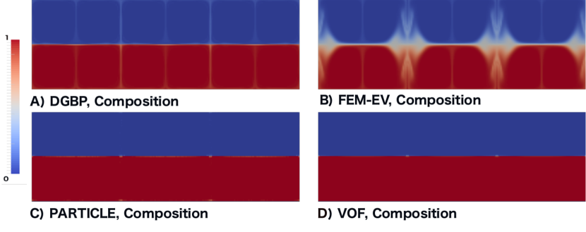
Figure 5: The composition at $t^{\prime}=0.05$ for $\mathrm{Ra}=10^{5}$ and $B=1.0$.

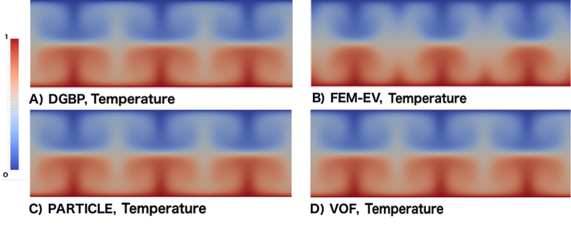
Figure 6: The temperature at $t^{\prime}=0.05$ for $\mathrm{Ra}=10^{5}$ and $B=1.0$.

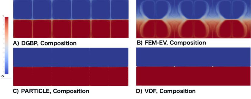
Figure 7: The composition at $t^{\prime}=0.1$ for $\mathrm{Ra}=10^{5}$ and $B=1.0$.

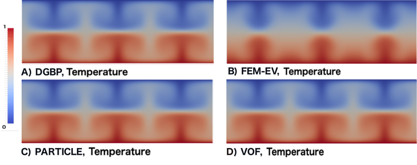
Figure 8: The temperature at $t^{\prime}=0.1$ for $\mathrm{Ra}=10^{5}$ and $B=1.0$.

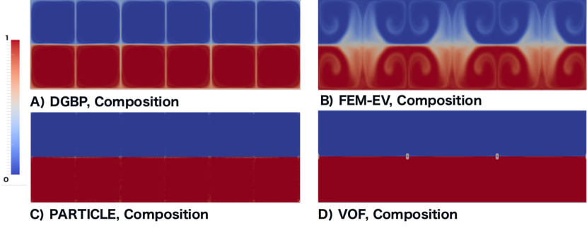
Figure 9: The composition at $t^{\prime}=0.15$ for $\mathrm{Ra}=10^{5}$ and $B=1.0$.

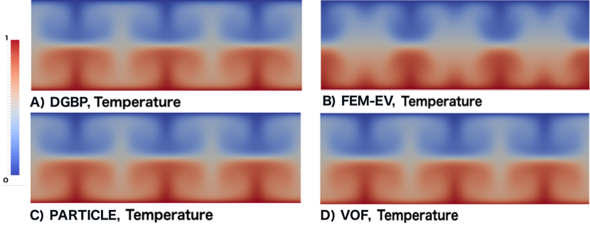
Figure 10: The temperature at $t^{\prime}=0.15$ for $\mathrm{Ra}=10^{5}$ and $B=1.0$.

4.2 The performance of the four algorithms for $\mathrm{Ra}=10^{5}$ and $\mathrm{B}=1.0$

In the following discussion we will use the following notation. We divide the computational domain $\Omega$ into two distinct regions $\Omega=\Omega_{1}\cup\Omega_{2}$ where $\Omega_{1}=\{(x,y):y>0.5\}$ denotes the upper half of the domain and $\Omega_{2}=\{(x,y):y<0.5\}$ denotes the lower half of the domain.

4.2.1 The performance of the DGBP algorithm

Figures 5–10 demonstrate that, at each time, the composition and temperature we computed with the DGBP, VOF and Particle algorithms are quite similar to each other, especially the temperature field. The flow is organized into relatively steady-state, discrete cells. Furthermore, the temperature fields we computed with these three algorithms are virtually indistinguishable from one another at each of the times shown. Note, however, that the DGBP algorithm has visible white bands at the interface between each convection cells. These are locations where the values of the composition field is approximately $C=0.5$ indicating that some of the composition field with value $C=1$ that was initially in the subdomain $\Omega_{1}$ has been entrained into the the flow in $\Omega_{2}$ and vice-versa. Although this enables one to easily see the convection cells it is due to numerical error.

(a) Particles initially in $\Omega_{1}$ at $t^{\prime}=0$

(b) Particles initially in $\Omega_{2}$ at $t^{\prime}=0$

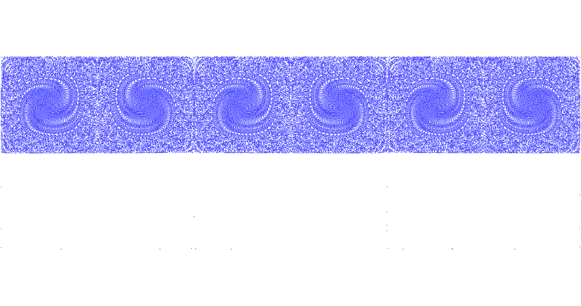
(c) Particles from $\Omega_{1}$ at $t^{\prime}=0.05$

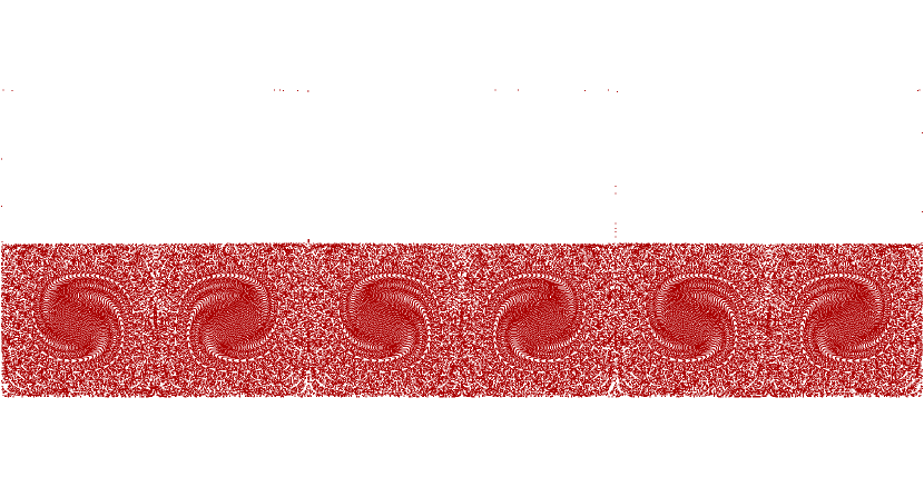
(d) Particles from $\Omega_{2}$ at $t^{\prime}=0.05$

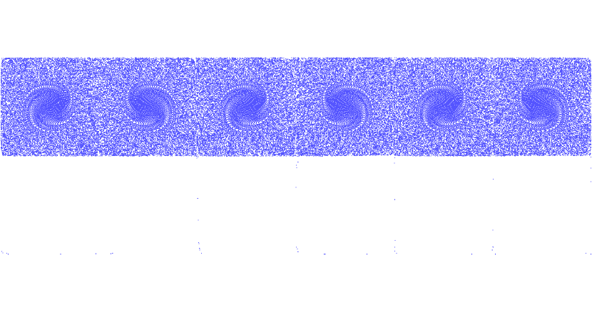
(e) Particles from $\Omega_{1}$ at $t^{\prime}=0.10$

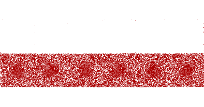
(f) Particles from $\Omega_{2}$ at $t^{\prime}=0.10$

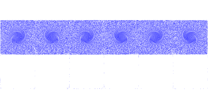
(g) Particles from $\Omega_{1}$ at $t^{\prime}=0.15$

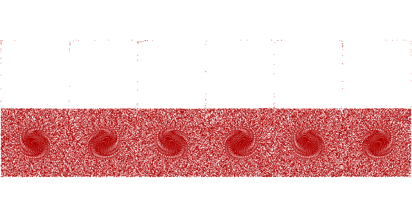
(h) Particles from $\Omega_{2}$ at $t^{\prime}=0.15$

Figure 11: The particles at times $t^{\prime}=0,\,0.05,\,0.10,\,0.15$ for a computation with $\mathrm{Ra}=10^{5}$ and $\mathrm{B}=1$ on a $192\times 64$ uniform grid. Initially the particles are distributed uniformly within each cell with $4\times 4=16$ particles per cell, so there are a total of 196,608 particles in the computation. Note that for $t^{\prime}>0.0$ some blue particles that should remain in $\Omega_{1}=\left[0,0.5\right]\times\left[0,3\right]$ are entrained in the flow along the boundaries of the convection cells and move into $\Omega_{2}=\left[0.5,1.0\right]\times\left[0,3\right]$ and vice-versa. See Table 2 for additional details.

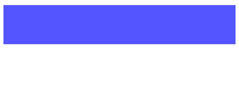
(a) Particles initially in $\Omega_{1}$ at $t^{\prime}=0$

(b) Particles initially in $\Omega_{2}$ at $t^{\prime}=0$

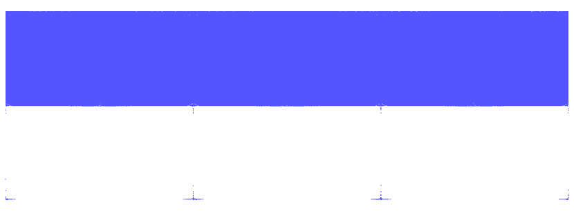
(c) Particles from $\Omega_{1}$ at $t^{\prime}=0.05$

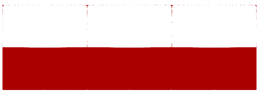
(d) Particles from $\Omega_{2}$ at $t^{\prime}=0.05$

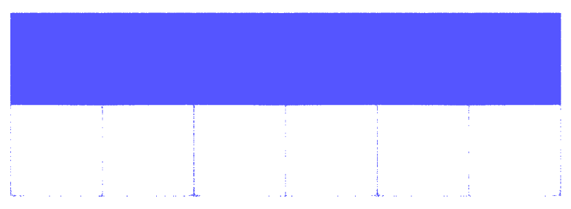
(e) Particles from $\Omega_{1}$ at $t^{\prime}=0.10$

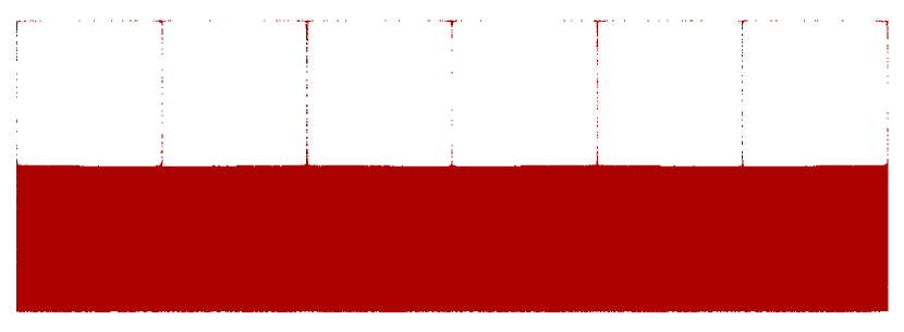
(f) Particles from $\Omega_{2}$ at $t^{\prime}=0.10$

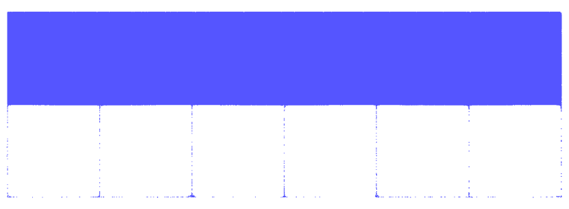
(g) Particles from $\Omega_{1}$ at $t^{\prime}=0.15$

(h) Particles from $\Omega_{2}$ at $t^{\prime}=0.15$

Figure 12: The particles at times $t^{\prime}=0,\,0.05,\,0.10,\,0.15$ for a computations with $\mathrm{Ra}=10^{5}$ and $\mathrm{B}=1$ on a $192\times 64$ uniform grid. Initially the particles are distributed uniformly within each cell with $16\times 16=256$ particles per cell, so there are a total of $3,145,728$ particles in the computation. Note that for $t^{\prime}>0.0$ some blue particles that should remain in $\Omega_{1}=\left[0,0.5\right]\times\left[0,3\right]$ are entrained in the flow along the boundaries of the convection cells and move into $\Omega_{2}=\left[0.5,1.0\right]\times\left[0,3\right]$ and vice-versa. See Table 3 for additional details.

Time	Direction	# entrained particles	Percentage
$t^{\prime}=0.05$	$\Omega_{1}\longrightarrow\Omega_{2}$	92	0.05%
	$\Omega_{2}\longrightarrow\Omega_{1}$	47	0.02%
$t^{\prime}=0.10$	$\Omega_{1}\longrightarrow\Omega_{2}$	128	0.07%
	$\Omega_{2}\longrightarrow\Omega_{1}$	117	0.06%
$t^{\prime}=0.15$	$\Omega_{1}\longrightarrow\Omega_{2}$	176	0.09%
	$\Omega_{2}\longrightarrow\Omega_{1}$	173	0.09%

Table 2: The number particles from each subdomain $\Omega_{1}$, $\Omega_{2}$, that have been entrained and advected into the other subdomain. This computation is on a uniform $192\times 64$ grid with $\mathrm{Ra}=10^{5}$ and $\mathrm{B=1}$ and, initially, $16$ particles per cell for a total of 196,608 particles.

.

4.2.2 The performance of the particle algorithm

In Figures 11 and 12 below the particles initially in $\Omega_{1}$ are blue and particles initially in $\Omega_{2}$ are red. It is difficult to see in Figures 5,  7, and 9, but in our computations some particles from $\Omega_{1}$ have been entrained and advected downward into $\Omega_{2}$, the red region. Similarly, some particles from $\Omega_{2}$ have been entrained and advected upward into from $\Omega_{1}$. This is easier to see in Figures 11 and 12.

Since the physical model is strongly stratified both the DGBP and particle algorithms are exhibiting non-physical features due to numerical errors intrinsic to the algorithm. As the time increases, this error increases; the white boundaries shown in the DGBP results increase with time and the number of particles in the wrong domain increases with time as shown in Tables 2 and 3.

Time	Direction	# entrained particles	Percentage
$t^{\prime}=0.05$	$\Omega_{1}\longrightarrow\Omega_{2}$	2412	0.05%
	$\Omega_{2}\longrightarrow\Omega_{1}$	764	0.02%
$t^{\prime}=0.10$	$\Omega_{1}\longrightarrow\Omega_{2}$	2648	0.08%
	$\Omega_{2}\longrightarrow\Omega_{1}$	947	0.03%
$t^{\prime}=0.15$	$\Omega_{1}\longrightarrow\Omega_{2}$	2941	0.09%
	$\Omega_{2}\longrightarrow\Omega_{1}$	1200	0.04%

Table 3: The number particles from each subdomain $\Omega_{1}$, $\Omega_{2}$, that have been entrained and advected into the other subdomain. This computation is on a uniform $192\times 64$ grid with $\mathrm{Ra}=10^{5}$ and $\mathrm{B=1}$ and initially $256$ particles per cell for a total of 3,145,728 particles.

4.2.3 The performance of the VOF method

In contrast, since it is an interface tracking method, the VOF algorithm maintains a sharp boundary at $y=0.5$. There are two small regions located at each intersection of the corners of two counter rotating convection cells. this is an area with a classic shear flow centered about a stagnation point that lies precisely at each corner. This is a very difficult flow in which to maintain a well defined interface. In future work we will examine the quality of the numerical solution at this point under grid resolution. In particular, since the VOF algorithm is only tracking a set of co-dimension one in a two dimensional flow (i.e, a one-dimensional curve in a two dimensional flow) this problem is an ideal candidate for adaptive mesh refinement. One of the key features of ASPECT is it’s adaptive mesh refinement capability. We have used it in other VOF computations to refine only about the interface. However, we decided that to do so here would be beyond the scope of this paper.

4.2.4 The performance of the FEM-EV algorithm

In stark contrast with the results of the three algorithms discussed above, the results for both the composition and temperature fields we computed with the FEM-EV algorithm are completely dissimilar from those computed with the other three algorithms at every time shown. In particular it is apparent that temperature we computed with the FEM-EV algorithm is far more diffusive than the temperature we computed with the other three algorithms. Similarly the composition we computed with the FEM-EV algorithm is completely dissimilar from the composition field we computed with the other three algorithms. In particular, the boundaries of the convection cells in both the upper and lower domains exhibit an unacceptably large amount of diffusion.

4.2.5 Summary

In summary, we conclude that for computations in regimes with strongly stratified flow through the transition regime, namely $\mathrm{B}>\mathrm{B}_{cr}$ the VOF algorithm, or any other high quality interface tracking algorithm, is the most appropriate method for modeling the interface between the chemical compositions. Our statement that the VOF algorithm will be superior to other algorithms in the transition regime is based on the first author’s experience with the VOF interface tracking algorithm in other settings [27, 28, 32, 17, 18]. We are planning future work to explicitly demonstrate that this statement is true for this class of problems.

4.3 Computations at $\mathrm{Ra}=10^{5}$ with $0\leq\mathrm{B}\leq 1.0$

In order to demonstrate the utility of this numerical methodology as a tool for studying thermochemical convection we computed a sequence of computations at $\mathrm{Ra}=10^{5}$ with a sequence of buoyancy numbers $B\,=0.0,\,0.1,\,0.2,\ldots,\,1.0$. This is covers the spectrum from the strongly stratified regime $B\geq\approx\,7.0$ through a transition regime $\approx 0.6\geq B\geq\approx 0.5$ to a regime that exhibits full kinematic mixing $\approx 0.4\geq B\geq\approx\,0.3$, to the limiting case of uniform chemical composition $\Delta\rho=0$ at $\mathrm{B}=0.0$; i.e., steady single-layer thermal convection.

For this study we decided to use only one of the four algorithms presented above, as one might chose to do for a research study of thermochemical convection. Our choice of algorithm was based on the following considerations.

1. As demonstrated in Figures 5–10 above, the FEM-EV algorithm produces computational results that are far too diffusive to be regarded as reliable, especially as the other three methods show the same general computational results over a very long time period; i.e., approximately $1900$ time steps.

2. For values of the Buoyancy number $\mathrm{B}<0.5$, the compositional field undergoes kinematic mixing on a scale for which it is inappropriate to use any interface tracing algorithm, including VOF. In particular we can rigorously quantify this by noting that the maximum curvature of the interface $\sigma_{max}$ goes to infinity $\sigma_{max}\to\infty$, and hence from the constraint we must also have the grid size $h\to 0$. See [34], [35] and [36] for details.

   
   

   The VOF algorithm is optimal for the range of values of $\mathrm{B}$ for which the compositional density fields are stably stratified through values of regimes in which the two compositions do not overturn and undergo kinematic mixing; i.e., $\mathrm{B}>\mathrm{B}_{cr}$ where $\mathrm{B}_{cr}$ is the value of $\mathrm{B}$ at which the compositional density fields overturn and kinematic mixing, begins to occur. As we have demonstrated in Figures 13 and 14, when $\mathrm{Ra}=10^{5}$ we find $\mathrm{B}_{cr}>\approx 0.4$ The DGBP and particle methods can be used in both the regimes, but they exhibit more numerical artifacts than the VOF algorithm for strongly stratified regime $B\geq\approx\,7.0$ and, more generally, in the transition or “oscillatory regime” $\approx\,7.0\geq\mathrm{B}>\mathrm{B}_{cr}$. We plan future work to further substantiate this latter claim.

3. For $\mathrm{B}\,<\,\mathrm{B}_{cr}$ the DGBP and Particle algorithms are likely to yield comparable computational results. For the following study we have chosen to use the DGBP algorithm. We have plans for future work that will include using the particle algorithm in ASPECT for similar computations.

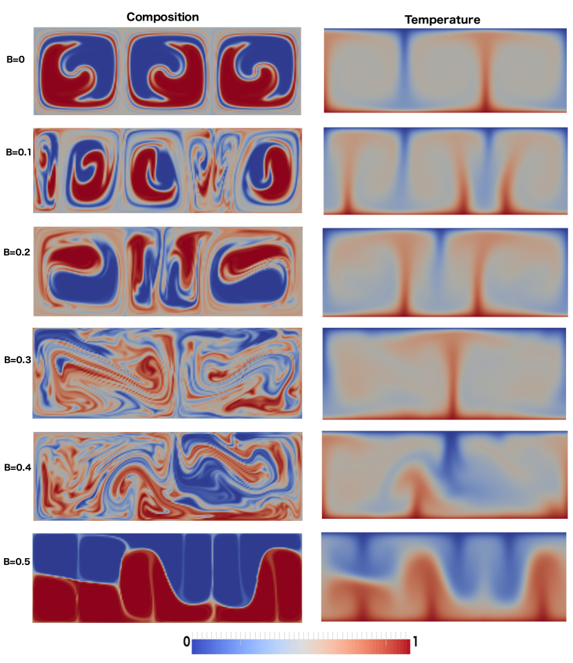
Figure 13: The composition and temperature at $t^{\prime}=0.15$ computed with the DGBP advection algorithm at $\mathrm{Ra}=10^{5}$ and $B=0.0,\,0.1,\,0.2,\,0.3,\,0.4,\,0.5$.

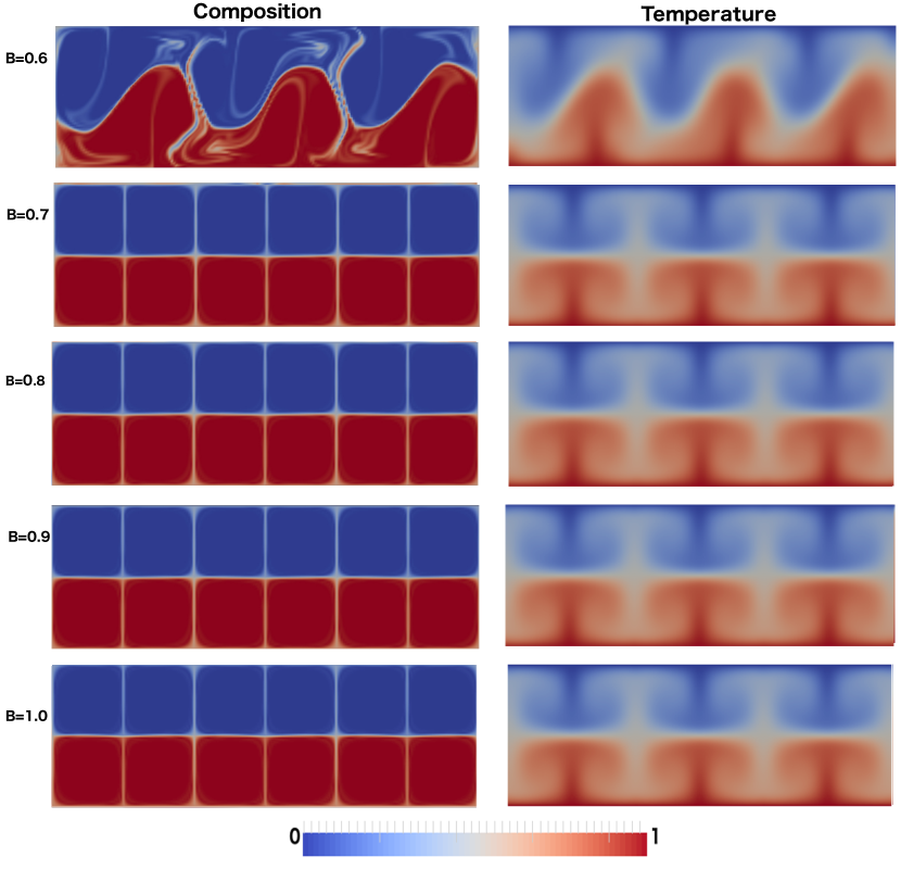
Figure 14: (A continuation of Figure 13) The composition and temperature at $t^{\prime}=0.15$ computed with the DGBP composition advection algorithm at $\mathrm{Ra}=10^{5}$ and $B=0.6,\,0.7,\,0.8,\,0.9,\,1.0$.

Our numerical results at the final dimensionless time of $t^{\prime}=0.15$ for $\mathrm{B}=0.0,\,0.1,\,0.2,\,\ldots,0.5$ are displayed in Figure 13, and for $B\,=\,0.6,\,0.7,\,\ldots,\,1.0$ in Figure 14. For $\mathrm{B}=0.0$ the compositional boundary is completely passive since $\Delta\rho=0$. Single layer thermal convection occurs with $\mathrm{Ra}=10^{5}$. At this Rayleigh number the convection is independent of time and passive kinematic mixing of the two layers occur in each cell. Eventually the composition in the entire layer will approach $C=1/2$. For $\mathrm{B}=0.1$ and $0.2$ the compositional barrier impedes the single layer convection, but the passive kinematic mixing in individual cells continues to dominate. For $\mathrm{B}=0.3$ and $0.4$ the flow becomes much more chaotic but is dominantly single layer convection. The chaotic behavior is attributed to a transition to a time dependent flow that enhances the kinematic mixing. For $\mathrm{B}=0.5$ and $0.6$ the compositional boundary is distorted but the flow is basically two layer convection. This range of $\mathrm{B}$ values give compositional structures that resemble the LLSVP structure of the Earth’s mantle. For $\mathrm{B}=0.7$ and larger the compositional boundary blocks vertical flows and two layer thermal convection occurs.

4.4 Relative Parallel Performance of the Algorithms

We conducted a strong scaling test to examine the degree to which the algorithms scale as the number of CPU processes or ‘cores’ increases in a high performance parallel computing environment. In a strong scaling test, a sequence of computations are made such that the size of the problem is fixed while the number of processor cores used for the computation increases [23, 25, 12].

In our test we computed the problem described in Section 4.1. The grid resolution was fixed at $768\times 256$ cells and we ran each method for $100$ time steps. In the computation with particles there were initially 16 equally spaced particles per cell. All of these computations were made on the high-performance computing cluster Maverick at the Texas Advance Computing Center.

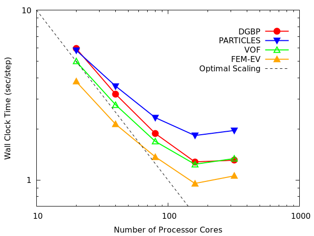
Figure 15: Strong scaling test for a fixed problem size of $768\times 256$ equally spaced square cells of size $h=1/256$ with $\mathrm{B}=1.0$ and $\mathrm{Ra}=10^{5}$. The flattening of the curves as the number of cores exceeds 80 cores (= 4 nodes) is expected. This is an indication that the cost of communication between nodes is becoming the dominant computational cost; i.e., there are too many nodes for the problem size.

The results are shown in Figures  15 and 16. For each computation, the elapsed wall clock time of the computation is measured and plotted. Figure 15 implies that of the different methods, the particle algorithm is more computationally expensive in comparison to the other algorithms. This is due to the additional cost associated with updating the location of the particles in time, and especially the communication cost incurred when passing particles across different MPI (Message Passing Interface) processes; see also Figure 1 of [12] for a more detailed analysis of the parallel scalability of the particle algorithm in ASPECT. Furthermore, Figure 15 shows that the DGBP and VOF algorithms have comparable wall clock times as we increase the number of processor cores. Although, FEM-EV is by far the fastest method, given the failure of this algorithm to accurately model the underlying physics of the problem this is a false economy.

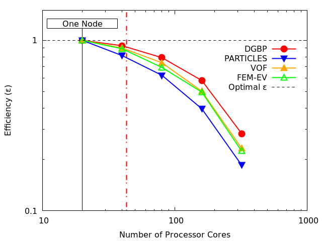
Figure 16: Strong scaling efficiency test for a fixed problem size. The 20 core case (1 node) is chosen to be the reference case in computing efficiency. The dashed horizontal line represents optimal scaling ($\epsilon=1$) and the dashed red vertical line is the parallelization limit, after which the cost of communicating between nodes begins to dominate the overall computational cost. The location of the vertical red line demonstrates that ASPECT, together any of the four algorithms, is approximately 90% efficient.

We also examined the relative scalable efficiency of the four methods when we use them in ASPECT. The efficiency $\epsilon=1$ is defined by

$$\epsilon=\frac{t_{ref}}{t}\frac{N_{ref}}{N_{Core}},$$ (62)

where $t$ is the elapsed time, $N_{Core}$ is the number of processor cores used, and $t_{ref}$ and $N_{ref}$ are the reference elapsed time and reference number of processor cores for each method [25]. In this strong scaling efficiency test, we chose a single node consisting of 20 processor cores as the reference core case and the measured wall clock time for each method on a single node as the reference times. The strong scaling efficiency results are shown in Figure 16. Assuming that a local minimum problem size $10^{5}$ FEM Degrees of Freedom (DoF) per core is the threshold for this scalability, as was determined in [1, 23], then for our fixed problem size of $768\times 256$ cells, we expect $43.3$ cores as the parallelization limit. The strong scaling results shown in Figures 15 and 16 demonstrate that each of the methods has good parallel scalability. Similar strong scaling results for ASPECT have also been published in [23] and [12].

5 Discussion

Our numerical results in Section 4.1 demonstrate the capabilities and limitations of the four algorithms we have used to model the motion of the compositional interface. The numerical results at $\mathrm{Ra}=10^{5}$ and $\mathrm{B}=1$ show that the FEM-EV advection algorithm produces extremely diffusive temperature and composition fields. Among these four algorithms, the FEM-EV and DGBP algorithms are both based on the Galerkin approach, which is a method for approximating the solution in the weak formulation. Since we applied the same time discretization for these two advection algorithms, the reason the results between the FEM-EV and DGBP advection algorithms are so different must be due to the differences in spacial discretization.

The major difference between the standard FEM and the DG method is that the DG method allows for discontinuities between elements. Therefore, it is well-known that DG is more suitable for problems with strong discontinuities or large gradients [3], such as occurs at the boundary between the compositional fields in our problem. In addition, in order to stabilize the numerical method, the FEM-EV algorithm uses an entropy viscosity technique, which is essentially adding an extra artificial diffusion term with variable artificial diffusivity $\nu_{h}^{k}(C)$ to the original pure advection equation (22) and resulting in equations (39) and (3.4.1).

It is apparent from the definition of the entropy viscosity in (40) [13] that the value of entropy viscosity decreases as the grid size $h$ decreases. Therefore, in order to reduce the amount of artificial diffusion, we have to reduce the grid size $h$ for a fixed polynomial basis, say a $Q_{2}$ finite element. Figure 17 shows that the maximum value of the entropy viscosity on the grid is greatly reduced from a computation on a grid of $96\times 32$ cells to a computation on a grid of $192\times 64$ cells for each time $t^{\prime}=0.05,\,0.10,\,0.15$ with the FEM-EV advection algorithm. However, if the numerical computations need a very long time to compute, we cannot neglect the accumulated error due to the artificial diffusion term with a relative large grid size $h$. In other words, if the final computation time $t$ is fixed, we may can determine an appropriate small $h$ such that there is less accumulated artificial diffusion which will not significantly change the final solution. However, to have numerical solutions with the same accuracy, a much large grid size $h$ is already enough for the other three advection algorithms. Therefore, the FEM-EV advection algorithm is the most diffusive method for a fixed $h$.

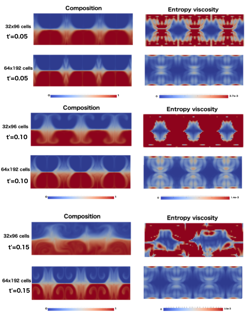
Figure 17: The composition and entropy-viscosity at time $t^{\prime}=0.05,\,0.10,\,0.15$ computed with the FEM-EV composition advection algorithm for $\mathrm{Ra}=10^{5}$ and $\mathrm{B}=1$.

In contrast, in the DGBP advection algorithm we first discretize the problem by applying a standard DG method with an upwind monotone flux. This does not explicitly add an artificial diffusion term to the advection equation. We then use a BP limiter in a post processing step in order to reduce or eliminate overshoot and undershoot in the DG solution near discontinuities in the composition variable $C$. In [50], it is shown that the BP limiter does not reduce the accuracy of the original DG solution. Also, numerical examples of the advection of non-diffusive fields in solid Earth geodynamics in [15] show that the DGBP solutions preserve a much sharper boundary as compared to the FEM-EV method on the same mesh with the same grid size.

However, for compared to the VOF interface tracking algorithm, $\mathrm{B}=1$ the DGBP advection algorithm does not maintain a sharp compositional boundary, across which the two compositional fields do not mix. The ability to maintain sharp boundaries through time in a computation is likely to influence conclusions related to the entrainment of compositional signals from boundary layers into rising thermal plumes. The computational results in [15] indicate that coupling the DGBP method to Adaptive Mesh Refinement (AMR) will limit the computational cost as mixing proceeds, at least until the mixing leads to compositional heterogeneity at all scales.

6 Conclusions

It is now widely accepted that compositional buoyancy plays an important role in mantle convection. Heterogeneous regions of the mantle can be produced in a variety of ways. One obvious source is the subducted lithosphere with the basaltic crust and a depleted complimentary mantle. After subduction there are two possible end member results of the interaction of the layered lithosphere with the convecting mantle. One is that the difference in densities between the subducted crust and the mantle results in a segregated (layered) mantle. The subducted crust could congregate in the deep mantle to create zero order layering. The alternative is that the mantle is homogenized by kinematic mixing.

The basaltic crust and mantle do not mix by material diffusion except on scales of centimeters to meters on geological time scales. Kinematic mixing is a tradeoff between the differential compositional buoyancy $\Delta\rho\,g$ that tends to segregate the two components and the thermal convective buoyancy $\rho_{0}\,\alpha\,\Delta T\,g$ that drives the kinematic mixing. There are two controlling non-dimensional parameters, the Rayleigh number $\mathrm{Ra}$ that determines the vigor of thermal convection and the buoyancy ratio $\mathrm{B}\,=\,\Delta\rho\,/\,\rho_{0}\,\alpha\,\Delta T$ that determines the relative strength of the stabilizing chemical buoyancy $\Delta\rho\,g$ versus the driving thermal buoyancy $\rho_{0}\,\alpha\,\Delta T\,g$. It has been the purpose of this paper to numerically study the segregation versus the kinematic mixing in a two component fluid for a range of buoyancy numbers $\mathrm{B}$ at a fixed Rayleigh number $\mathrm{Ra}$. In order to do so, we first compared the accuracy and quality of the computational solution obtained from computing the compositional boundary with four alternative approaches in a strongly stably stratified regime at a single, fixed, Rayleigh number; i.e., for extremely stable compositional segregation.

Many previous computations of thermo-chemical convection have been carried out. However, some numerical methods for modeling the compositional interface are too diffusive, resulting in artificial mixing, which leads to inaccurate computational results. Since the compositional fields are non-diffusive, ideally the numerical methodology should be able to track the sharp boundary between each field for all values of $\mathrm{B}$ at a fixed Rayleigh number $\mathrm{Ra}$. However, the extremely small length scales prevalent in fully developed kinematic mixing required us to choose a different numerical method than the method we found to be optimal for modeling the interface at values of $\mathrm{B}$ above that value $\mathrm{B}_{cr}$ at which the interface turns over and kinematics mixing develops.

In this article we describe in detail three alternative numerical methods to reduce numerical diffusion while modeling the advection of two compostional fields; namely, a Discontinuous Galerkin method with a Bound Preserving limiter (DGBP), a Volume-of-Fluid (VOF) interface tracking algorithm, and the advection of particles that carry a scalar quantity representing the location of each compositional field. The first two of these methods are relatively new in the computational mantle convection community. All three methods have been implemented in the open source Finite Element (FEM) code ASPECT for modeling processes that occur in mantle convection. ASPECT is freely available from the Computational Infrastructure for Geodynamics. We compare the performance of these three alternative methods with the advection method that was first developed for modeling the advection of a compostional field in ASPECT. This method is based on a high-order accurate finite element advection algorithm with an artificial viscosity stabilization technique known as ‘Entropy Viscosity’ (FEM-EV). We use ASPECT to compute the velocity, pressure, and temperature fields associated with the underlying flow with each of these four methods.

In order to examine the relative performance of these four methods, we have considered two-dimensional thermal convection in a fluid layer heated from below with an initial compositional barrier between the upper and lower half of the layer with Buoyancy number $\mathrm{B}=1$ and Rayleigh number $\mathrm{Ra}=10^{5}$. This is a regime for which the initial stratification of the compositional fields persists indefinitely. The numerical results we computed with the FEM entropy viscosity-based method are far too diffusive to produce meaningful results. We argue that this is, at least in part, due to the additional artificial diffusion that is added by the entropy viscosity method in order to stabilize the advection algorithm. In contrast, the other three algorithms produce nearly identical temperature fields, even at relatively late times; e.g., after approximately 19000 time steps.

On the other hand, the compositional field computed with DGBP, VOF, and the particles have distinct differences. Computations made with the DGBP method exhibit some amount of each compositional field that is (numerically) entrained within the other compositional field and advects along the boundary of the convection cells in the wrong compostional domain. The particle method exhibits a similar phenomenon, in which some particles representing the denser fluid are entrained in the upper, less dense fluid and advect along the boundary of the convection cells in the wrong compostional domain and, similarly, a small number of particles representing the less dense fluid are entrained in the lower, denser fluid and are advected along the boundary of the convection cells but in the wrong compostional domain. Finally, we found that the VOF method maintains a sharp interface between the two compositions on a subgrid scale throughout the computation. There is a small numerical error on the interface at two stagnation points that form at the intersection of four counter rotating convection cells. At these two points the flow is a classic shear flow centered on the interface, which is notoriously difficult to model. Our conclusion is that of the three algorithms we tested, in this regime the VOF interface tracking algorithm yields the most accurate numerical results.

We then computed the same problem in the same computational domain with Rayleigh number $\mathrm{Ra}=10^{5}$ but for a range of buoyancy numbers $\mathrm{B}=0.0,\,0.1,\ldots,\,1.0$ using the DGBP method in order to demonstrate the utility of this method when the stratified layer overturns and begins to mix. This is a regime for which the VOF method is not suitable without an untenably large increase in the resolution of the underlying grid. In our judgment the DGBP algorithm was one of two approaches that we could have used to study the basic mixing versus segregation process; i.e., over a wide range of buoyancy numbers $\mathrm{B}$ for a given Rayleigh number. We believe we could also have used the particle method for this study. This will be the subject of future work.

The results of our computations are summarized in Figures 13 and 14. There are basically four modes depending on the value of the buoyancy parameter $\mathrm{B}$. Our results are for $\mathrm{Ra}\,=\,10^{5}$ based on the full layer thickness. With no chemical buoyancy $\mathrm{B}\,=\,0$, a time independent cellular convection pattern develops and there is no mixing between adjacent cells. For small chemical buoyancy, $\mathrm{B}\,=\,0.1$ and $0.2$, this flow is maintained. Kinematic mixing takes place in the individual cells but is relatively slow. For $\mathrm{B}\,=\,0.3$ and $0.4$ the flow is quite different. The chemical buoyancy has resulted in unsteady flows that greatly enhance the kinematic mixing but do not block the vertical flows between the upper and lower layers. At $\mathrm{B}\,=\,0.5$ and $0.6$ there is sufficient chemical buoyancy to impede vertical flow between the two layers but the compositional buoyancy does not prevent a significant vertical displacement of the compositional boundary. Relatively little mixing between the layers is seen at this time and the structure resembles that of low shear velocity provinces. For $\mathrm{B}\,=\,0.7$ to $1.0$ the chemical stabilizing buoyancy is sufficiently strong to block vertical flows between the upper and lower layers and the compositional boundary is essentially flat and thermal convection occurs in two independent layers.

References

- 1. Wolfgang Bangerth, Carsten Burstedde, Timo Heister, and Martin Kronbichler. Algorithms and data structures for massively parallel generic adaptive finite element codes. ACM Transactions on Mathematical Software (TOMS), 38(2):14, 2011.
- 2. Kevin Burke, Bernhard Steinberger, Trond H Torsvik, and Mark A Smethurst. Plume generation zones at the margins of large low shear velocity provinces on the core–mantle boundary. Earth and Planetary Science Letters, 265(1):49–60, 2008.
- 3. Bernardo Cockburn, George E. Karniadakis, and Chi-Wang Shu. The Development of Discontinuous Galerkin Methods, pages 3–50. Springer Berlin Heidelberg, Berlin, Heidelberg, 2000.
- 4. Bernardo Cockburn and Chi-Wang Shu. The local discontinuous Galerkin method for time-dependent convection-diffusion systems. SIAM Journal on Numerical Analysis, 35(6):2440–2463, 1998.
- 5. Philip Colella. Multidimensional upwind methods for hyperbolic conservation laws. J. Comput. Phys., 87:171–200, 1990.
- 6. Sanne Cottaar and Barbara Romanowicz. An unusually large ULVZ at the base of the mantle near Hawaii. Earth and Planetary Science Letters, 355:213–222, 2012.
- 7. Anne Davaille. Two-layer thermal convection in miscible viscous fluids. Journal of Fluid Mechanics, 379:223–253, 1999.
- 8. Jean Donea and Antonio Huerta. Steady Transport Problems. John Wiley and Sons, 2005.
- 9. T. Duretz, D. A. May, T. V. Gerya, and P. J. Tackley. Discretization errors and free surface stabilization in the finite difference and marker-in-cell method for applied geodynamics: A numerical study. Geochemistry, Geophysics, Geosystems, 12(7), 2011. Q07004.
- 10. Scott W French and Barbara Romanowicz. Broad plumes rooted at the base of the Earth’s mantle beneath major hotspots. Nature, 525(7567):95–99, 2015.
- 11. A Galsa, M Herein, L Lenkey, MP Farkas, and G Taller. Effective buoyancy ratio: a new parameter for characterizing thermo-chemical mixing in the Earth’s mantle. Solid Earth, 6(1):93–105, 2015.
- 12. Rene Gassmöller, Eric Heien, Elbridge Gerry Puckett, and Wolfgang Bangerth. Flexible and scalable particle-in-cell methods for massively parallel computations. ACM Transactions on Mathematical Software (2016) (submitted), 2016.
- 13. Jean-Luc Guermond and Richard Pasquetti. Entropy viscosity method for high-order approximations of conservation laws. In Spectral and high order methods for partial differential equations, pages 411–418. Springer, 2011.
- 14. Jean-Luc Guermond, Richard Pasquetti, and Bojan Popov. Entropy viscosity method for nonlinear conservation laws. Journal of Computational Physics, 230(11):4248 – 4267, 2011. Special issue High Order Methods for CFD Problems.
- 15. Ying He, Elbridge Gerry Puckett, and Magali I. Billen. A discontinuous Galerkin method with a bound preserving limiter for the advection of non-diffusive fields in solid Earth geodynamics. Physics of the Earth and Planetary Interiors, 263:23–37, 2017.
- 16. T. Heister, J. Dannberg, R. Gassmöller, and W. Bangerth. High Accuracy Mantle Convection Simulation through Modern Numerical Methods. II: Realistic Models and Problems. ArXiv e-prints, February 2017.
- 17. Leroy F. Henderson, Phillip Colella, and Elbridge Gerry Puckett. On the refraction of shock waves at a slowfast gas interface. J. Fluid Mech., 224:1–27, March 1991.
- 18. Leroy F. Henderson and Elbridge Gerry Puckett. The refraction of shock pairs. Shock Waves, 24(6):553–572, November 2014.
- 19. Jan S Hesthaven and Tim Warburton. Nodal discontinuous Galerkin methods, volume 54 of Texts in Applied Mathematics. Springer, New York, 2008.
- 20. R Huber and R Helmig. Multiphase flow in heterogeneous porous media: A classical finite element method versus an implicit pressure–explicit saturation-based mixed finite element–finite volume approach. International Journal for Numerical Methods in Fluids, 29(8):899–920, 1999.
- 21. Louise H Kellogg. Mixing in the mantle. Annual Review of Earth and Planetary Sciences, 20(1):365–388, 1992.
- 22. Louise H Kellogg, Bradford H Hager, and Rob D van der Hilst. Compositional stratification in the deep mantle. Science, 283(5409):1881–1884, 1999.
- 23. M. Kronbichler, T. Heister, and W. Bangerth. High accuracy mantle convection simulation through modern numerical methods. Geophysical Journal International, 191(1):12–29, 2012.
- 24. Randall J. LeVeque. High-resolution conservative algorithms for advection in incompressible flow. SIAM J. Numer. Anal., 33(2):627–665, April 1996.
- 25. Hiroaki Matsui, Eric Heien, Julien Aubert, Jonathan M. Aurnou, Margaret Avery, Ben Brown, Bruce A. Buffett, Friedrich Busse, Ulrich R. Christensen, Christopher J. Davies, Nicholas Featherstone, Thomas Gastine, Gary A. Glatzmaier, David Gubbins, Jean-Luc Guermond, Yoshi-Yuki Hayashi, Rainer Hollerbach, Lorraine J. Hwang, Andrew Jackson, Chris A. Jones, Weiyuan Jiang, Louise H. Kellogg, Weijia Kuang, Maylis Landeau, Philippe Marti, Peter Olson, Adolfo Ribeiro, Youhei Sasaki, Nathanaël Schaeffer, Radostin D. Simitev, Andrey Sheyko, Luis Silva, Sabine Stanley, Futoshi Takahashi, Shin-ichi Takehiro, Johannes Wicht, and Ashley P. Willis. Performance benchmarks for a next generation numerical dynamo model. Geochemistry, Geophysics, Geosystems, 17(5):1586–1607, 2016.
- 26. Allen K McNamara and Shijie Zhong. Thermochemical structures within a spherical mantle: Superplumes or piles? Journal of Geophysical Research: Solid Earth, 109(B07402), 2004.
- 27. G. H. Miller and E. G. Puckett. Edge effects in molybdenum-encapsulated molten silicate shock wave targets. J. Appl. Phys., 75(3):1426–1434, February 1994.
- 28. G. H. Miller and E. G. Puckett. A high-order godunov method for multiple condensed phases. J. Comput. Phys., 128(1):134–164, August 1996.
- 29. Nancy L Montague and Louise H Kellogg. Numerical models of a dense layer at the base of the mantle and implications for the geodynamics of D”. Journal of Geophysical Research: Solid Earth, 105(B5):11101–11114, 2000.
- 30. James Edward Pilliod. An analysis of piecewise linear interface reconstruction algorithms for volume-of-fluid methods. MS Thesis, Graduate Group in Applied Mathematics, University of California, Davis, September 1992.
- 31. James Edward Pilliod and Elbridge Gerry Puckett. Second-order accurate volume-of-fluid algorithms for tracking material interfaces. J. Comput. Phys., 199(2):465–502, September 2004.
- 32. E. G. Puckett, A. S. Almgren, J. B. Bell, D. L. Marcus, and W. J. Rider. A high-order projection method for tracking fluid interfaces in variable density incompressible flows. J. Comput. Phys., 130(2):269–282, January 1997.
- 33. Elbridge Gerry Puckett. A volume-of-fluid interface tracking algorithm with applications to computing shock wave refraction. In Proceedings of the Fourth International Symposium on Computational Fluid Dynamics, pages 933–938, 1991.
- 34. Elbridge Gerry Puckett. On the second-order accuracy of volume-of-fluid interface reconstruction algorithms: Convergence in the max norm. CAMCoS, 5(1):99–148, February 2010.
- 35. Elbridge Gerry Puckett. A volume-of-fluid interface reconstruction algorithm that is second-order accurate in the max norm. CAMCoS, 5(2):199–220, 2010.
- 36. Elbridge Gerry Puckett. On the second-order accuracy of volume-of-fluid interface reconstruction algorithms II: An improved constraint on the cell size. CAMCoS, 8(1):123–158, January 2014.
- 37. W.H. Reed and T.R. Hill. Triangular mesh methods for the neutron transport equation. Technical Report LA-UR–73-479, Los Alamos Scientific Lab, Oct 1973.
- 38. Gerald Schubert, D. L. Turcotte, and P. Olson. Mantle convection in the Earth and planets. Cambridge University Press, 2001.
- 39. JW Sheldon, WT Cardwell Jr, et al. One-dimensional, incompressible, noncapillary, two-phase fluid flow in a porous medium. Petroleum Transactions, AIME, 216:290–296, 1959.
- 40. Chi-Wang Shu. Discontinuous Galerkin methods for time-dependent convection dominated problems: Basics, recent developments and comparison with other methods. In Building Bridges: Connections and Challenges in Modern Approaches to Numerical Partial Differential Equations, pages 369–397. Springer, 2016.
- 41. Paul J Tackley. Dynamics and evolution of the deep mantle resulting from thermal, chemical, phase and melting effects. Earth-Science Reviews, 110(1):1–25, 2012.
- 42. Paul J. Tackley and Scott D. King. Testing the tracer ratio method for modeling active compositional fields in mantle convection simulations. Geochemistry, Geophysics, Geosystems, 4(4), 2003. Q8302.
- 43. Eh Tan and Michael Gurnis. Metastable superplumes and mantle compressibility. Geophysical Research Letters, 32(20), 2005.
- 44. Marcel Thielmann, DA May, and BJP Kaus. Discretization errors in the hybrid finite element particle-in-cell method. Pure and Applied Geophysics, 171(9):2165–2184, 2014.
- 45. Sean J. Trim and Julian P. Lowman. Interaction between the supercontinent cycle and the evolution of intrinsically dense provinces in the deep mantle. Journal of Geophysical Research: Solid Earth, 121(12):8941–8969, 2016. 2016JB013285.
- 46. SJ Trim, PJ Heron, C Stein, and JP Lowman. The feedback between surface mobility and mantle compositional heterogeneity: Implications for the Earth and other terrestrial planets. Earth and Planetary Science Letters, 405:1–14, 2014.
- 47. Donald L Turcotte and Gerald Schubert. Geodynamics. Cambridge University Press, Cambridge, 3rd edition, 2014.
- 48. John Von Neumann and Robert D Richtmyer. A method for the numerical calculation of hydrodynamic shocks. Journal of Applied Physics, 21(3):232–237, 1950.
- 49. Gerhard Wanner and Ernst Hairer. Solving ordinary differential equations II, volume 14 of Springer Series in Computational Mathematics. Springer-Verlag Berlin Heidelberg, 1991.
- 50. Xiangxiong Zhang and Chi-Wang Shu. On maximum-principle-satisfying high order schemes for scalar conservation laws. Journal of Computational Physics, 229(9):3091 – 3120, 2010.