Cosmological Production of Electroweak Monopole

Abstract

We discuss the cosmological production and the successive evolution of the electroweak monopole in the standard model, and estimate the remnant monopole density at present universe. We confirm that, although the electroweak phase transition is of the first order, it is very mildly first order. So, the monopole production arises from the thermal fluctuations of the Higgs field after the phase transition, not the vacuum bubble collisions during the phase transition. Moreover, while the monopoles are produced copiously around the Ginzburg temperature $T_{G}\simeq 59.6~{}{\rm TeV}$, most of them are annihilated as soon as created. This annihilation process continues very long, untill the temperature cools down to about 29.5 MeV. As the result the remnant monopole density in the present universe becomes very small, of $10^{-11}$ of the critical density, too small to affect the standard cosmology and too small comprise a major component of dark matter. We discuss the physical implications of our results on the ongoing monopole detection experiments, in particular on MoEDAL, IceCube, ANTARES, and Auger.

I Introduction

Ever since Dirac has proposed the Dirac monopole generalizing the Maxwell’s theory, the monopole has become an obsession theoretically as well as experimentally dirac . After the Dirac monopole we have had the Wu-Yang monopole wu , the ’t Hooft-Polyakov monopole thooft , the grand unification (Dokos-Tomaras) monopole dokos , and the electroweak (Cho-Maison) monopole plb97 ; yang ; epjc15 ; ellis ; plb16 . But none of them except for the electroweak monopole might become realistic enough to be discovered.

Indeed the Dirac monopole in electrodynamics should transform to the electroweak monopole after the unification of the electromagnetic and weak interactions, and the Wu-Yang monopole in QCD is supposed to make the monopole condensation to confine the color. Moreover, the ’t Hooft-Polyakov monopole exists in an hypothetical theory, and the grand unification monopole which could have been amply produced at the grand unification scale in the early universe probably has become completely irrelevant at present universe after the inflation.

This makes the electroweak monopole the only realistic monopole we could ever hope to detect. This has made the experimental confirmation of the electroweak monopole one of the most urgent issues in the standard model, after the discovery of the Higgs particle at LHC. In fact the newest MoEDAL (“the magnificent seventh”) detector at LHC is actively searching for the monopole medal1 ; medal2 .

On the other hand, MoEDAL may have no chance to detect the electroweak monopole if the mass becomes larger than 6.5 TeV, because the present 13 TeV LHC is expected to produce the monopole pair only when the mass is smaller than 6.5 TeV. In this case we may have to search for the remnant monopole in the present universe which survived from the early universe, or else wait for the next LHC upgrading. So it is wise to adopt two track strategy to detect the monopole, the LHC-produced monopoles and the remnant monopoles in the present universe. In this sense it is encouraging that IceCube and similar detectors, e.g., ANTARES, Auger, are aiming to detect the remnant monopoles icecube ; antares ; auger .

To detect the remnant monopoles, however, it is important for us to know the monopole density at present universe. There have been discussions on the impact of the monopoles in cosmology kibble ; pres ; guth ; zurek , but most of the discussions have been on the grand unification monopoles. The general consensus is that the grand unification monopoles would have overclosed the universe without inflation, but inflation might have completely diluted them in such a way that the grand unification monopole could have no visible impact on the present universe infl .

For the electroweak monopole, however, the situation has not been so clear kriz ; zel ; and ; koba . There have been claims that the electroweak monopoles could also overclose the universe zel , but we need a more accurate discussion on this issue. The purpose of this paper is to discuss the monopole production after the electroweak phase transition and the successive cosmological evolution of the monopoles, to predict the remnant monopole density at present universe and to discuss the cosmological implications of the electroweak monopole.

Our analysis confirms that the electroweak phase transition is of the first order, but the energy barrier at the critical temperature is negligibly small that it can be treated as the second order for all practical purposes. So we argue that the monopole production comes from the thermal fluctuations of the Higgs field after the phase transition, not the vacuum bubble collosions during the phase transition. As importantly, we show that although the electroweak monopoles are produced copiously around the Ginzburg temperature $T_{G}\simeq 60~{}{\rm GeV}$, they are annihilated as soon as created. And this annihilation process continues very long time, till the universe cools down to around 29.5 MeV. This is basically because the monopole-antimonopole attraction is much bigger, $1/\alpha$-times bigger, than the electromagnetic interaction.

As the result the density of the electroweak monopoles at present universe turns out to be very small, about $10^{-11}$ of the critical density. This assures that, unlike the grand unification monopole, the electroweak monopole does not cause any problem in cosmology. Moreover, this tells that there is no possibility that the electroweak monopoles could become the dark matter of the universe.

Nevertheless we find that there are enough remaining monopoles in the present universe which we could detect without much difficulty. We estimate the monopole number density at present universe to be roughly $6.1\times 10^{-22}/{\rm cm^{3}}$. Intuitively, this means that there are roughly $6.6\times 10^{7}$ monopoles per unit volume of the earth in the universe.

Although the electroweak monopole does not alter the standard cosmology, it could play important roles in cosmology. First, as the heaviest stable particle the remnant monopoles could generate the density perturbation and become the seeds of the large scale structures of the universe. Second, accelerated by the intergalactic magnetic field, they become the natural source of the ultra-relativistic cosmic rays. Third, they could induce the electroweak baryogenesis.

The paper is organized as follows. In Section II we review the fundamental properties of the electroweak monopole for later purpose. In Section III we discuss the electroweak phase transition in detail. In Section IV we discuss the monopole production after the phase transition in detail, both in the first order phase transition and the second order approximation. In Section V we discuss the evolution of the monopoles and estimate the remnant monopole density at present universe. In Section VI we compare our result with the Parker bound on average intergalactic magnetic field in the universe. In the last section we discuss the physical implications of our results, in particular on the ongoing MoEDAL, IceCube, and similar monopole detection experiments.

II Electroweak Monopole: A Review

Before we estimate the electroweak monopole density at present universe, we need to clarify the existing confusions and misunderstandings on the monopole. For this reason we briefly review the electroweak monopole in the standard model first.

Consider the Weinberg-Salam model,

$${\cal L}=-|{\cal D}_{\mu}\phi|^{2}-\frac{\lambda}{2}\Big{(}\phi^{\dagger}\phi-\frac{\mu^{2}}{\lambda}\Big{)}^{2}-\frac{1}{4}\vec{F}_{\mu\nu}^{2}-\frac{1}{4}G_{\mu\nu}^{2},$$

$${\cal D}_{\mu}\phi=\big{(}\partial_{\mu}-i\frac{g}{2}\vec{\tau}\cdot\vec{A}_{\mu}-i\frac{g^{\prime}}{2}B_{\mu}\big{)}\phi,$$ (1)

where $\phi$ is the Higgs doublet, $\vec{A}_{\mu}$ and $B_{\mu}$ are the SU(2) and U(1) gauge potentials. Introducing the Higgs field $\rho$ and the $CP^{1}$ field $\xi$ by

$$\phi=\dfrac{1}{\sqrt{2}}\rho~{}\xi,~{}~{}~{}(\xi^{\dagger}\xi=1),$$ (2)

we have

$${\cal L}=-\frac{1}{2}{(\partial_{\mu}\rho)}^{2}-\frac{\rho^{2}}{2}{|{\cal D}_{\mu}\xi|}^{2}-\frac{\lambda}{8}\big{(}\rho^{2}-\rho_{0}^{2}\big{)}^{2}$$

$$-\frac{1}{4}{\vec{F}}_{\mu\nu}^{2}-\frac{1}{4}G_{\mu\nu}^{2},~{}~{}~{}~{}(\rho_{0}^{2}=\frac{2\mu^{2}}{\lambda}).$$ (3)

With the ansatz

$$\rho=\rho(r),~{}~{}~{}\xi=i\left(\begin{array}[]{cc}\sin(\theta/2)~{}e^{-i\varphi}\\ -\cos(\theta/2)\end{array}\right),$$ (6)

$$\vec{A}_{\mu}=\frac{1}{g}A(r)\partial_{\mu}t~{}\hat{r}+\frac{1}{g}(f(r)-1)~{}\hat{r}\times\partial_{\mu}\hat{r},$$

$$B_{\mu}=\frac{1}{g^{\prime}}B(r)\partial_{\mu}t-\frac{1}{g^{\prime}}(1-\cos\theta)\partial_{\mu}\varphi,$$ (7)

we have the dyon solution of the standard model dressed by the W-boson, Z-boson, and Higgs field, which becomes the monopole solution with $A=B=0$. The singular monopole solution is shown in Fig. 1 plb97 ; yang ; epjc15 .

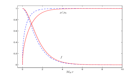
Figure 1: The finite energy electroweak monopole solution. The solid line (red) represents the regularized monopole and the dotted (blue) line represents the singular electroweak monopole.

The first and (most serious) misunderstanding on the electroweak monopole is the existence. This, of course, is the fundamental issue. It has been asserted that the vacuum of the Weinberg-Salam model does not allow the monopole topology nogo . If so, there would be no phase transition which could produce the monopole, and thus no cosmic production of the monopole.

Actually there are two questions here. As we know, the Dirac monopole in electrodynamics is optional, not a necessity, so that it does not have to exist. This is because the electromagnetic U(1) allows the monopole only when it becomes non-trivial. So the first question is whether the standard model could admit the monopole topology or not. The second question is, if the monopole topology is consistent with the standard model, is the monopole optional or not.

Obviously the existence of the monopole assures that the standard model could be made to admit the monopole topology plb97 ; yang ; epjc15 . So the remaining question is if this monopole topology is optional or not. It is not optional. The electroweak monopole must exist, if the standard model is correct.

To see this notice that in the ansatz (7) the hypercharge U(1) is made to be non-trivial, which was why the electroweak monopole could exist. So we have to find the reason why the hypercharge U(1) in the standard model must be non-trivial. This follows from two facts. First, the electromagnetic U(1) in the standard model is given by the linear combination of the U(1) subgroup of SU(2) and the hypercharge U(1). Second, the U(1) subgroup of SU(2) is non-trivial. In this case the mathematical consistency requires the hypercharge U(1), and consequently the electromagnetic U(1), to be non-trivial.

But, of course, this has to be confirmed by experiment. This makes the discovery of the monopole, not the Higgs particle, the final (and topological) test of the standard model. This is why the electroweak monopole is so important.

The second confusion is the assertion that, even if it exists, there would be no fundamental difference between the Dirac monopole and the electroweak monopole. So the important question here is whether there is any characteristic feature of the electroweak monopole which is different from the Dirac monopole. We have to know this to tell the monopole, when discovered, is the Dirac monopole or the electroweak monopole. The answer is yes, there is an unmistakable difference. The electroweak monopole carries the magnetic charge twice bigger than the Dirac monopole plb97 ; epjc15 .

The reason is simple. It is well known that the magnetic charge of Dirac monopole must be a multiple of $2\pi/e$. This is because the period of the electromagnetic U(1) is $2\pi$. However, in the course of the electroweak unification the period of electromagnetic U(1) becomes $4\pi$, because the period of the U(1) subgroup of SU(2) becomes $4\pi$. Consequently the magnetic charge $g_{m}$ of the electroweak monopole must be a multiple of $4\pi/e$.

The third misunderstanding is that we can not estimate the mass of the electroweak monopole, because the electroweak monopole has the point singularity at the origin which makes the energy infinite. Obviously the monopole mass is the most important piece of information from the experimental point of view. There was no way to predict the mass of the Dirac monopole theoretically, and this has made the monopole detection a blind search in the dark room without any theoretical lead.

But this assertion is not true, either. Since the mass of the electroweak monopole is a crucial information for us to estimate the monopole density in the universe, it is worth to discuss this issue in more detail. As a hybrid between the Dirac and ’t Hooft-Polyakov monopoles, the electroweak monopole does have a singularity at the origin which makes the energy divergent. Nevertheless we could easily guess the mass to be of the order of 10 TeV, roughly $4\pi/e^{2}$ times the W-boson mass. This is because the monopole mass essentially comes from the same Higgs mechanism which generates the W-boson mass, except that the monopole potential couples to the Higgs multiplet magnetically, not electrically, with the strength $4\pi/e$ plb97 ; epjc15 .

Another way to estimate the mass is to regularize the monopole to make the energy finite epjc15 . To do this let us modify (3) to the following effective Lagrangian with a non-trivial permittivity $\epsilon$ for the hypercharge U(1) gauge field

$${\cal L}_{eff}=-\frac{1}{2}{(\partial_{\mu}\rho)}^{2}-\frac{\rho^{2}}{2}{|{\cal D}_{\mu}\xi|}^{2}-\frac{\lambda}{8}\big{(}\rho^{2}-\rho_{0}^{2}\big{)}^{2}$$

$$-\frac{1}{4}{\vec{F}}_{\mu\nu}^{2}-\frac{\epsilon(\rho)}{4}G_{\mu\nu}^{2}.$$ (8)

The effective Lagrangian still retains the SU(2) $\times$ U(1) gauge symmetry. Moreover, when $\epsilon=1$, the Lagrangian reproduces the standard model. So this modification affects only the short distance behavior, if $\epsilon$ approaches to the unit asymptotically.

To see how $\epsilon$ mimics the quantum correction and regularize the monopole, notice that the rescaling of $B_{\mu}$ to $B_{\mu}/g^{\prime}$ changes $g^{\prime}$ to $g^{\prime}/\sqrt{\epsilon}$. So $\epsilon$ effectively changes the hypercharge U(1) gauge coupling $g^{\prime}$ to the “running” coupling $\bar{g}^{\prime}=g^{\prime}/\sqrt{\epsilon}$. This means that, by making $\bar{g}^{\prime}$ infinite (requiring $\epsilon$ vanishing) at the origin, we can remove the singularity of the monopole. Moreover, with $\epsilon(\infty)=1$, we can reproduce the singular monopole asymptotically. In fact, with $\epsilon=(\rho/\rho_{0})^{8}$, we have the regularized monopole solution which has the energy around 7 TeV epjc15 ; plb16 . This is shown in Fig. 1. Notice that asymptotically the regularized monopole looks almost identical to the singular monopole.

The regularized monopole energy, of course, depends on the functional form of $\epsilon$, so that we could change the energy changing $\epsilon$. But this also affects other things, for example the Higgs to two photon decay rate. And recently Ellis and collaborators noticed that, choosing a more realistic $\epsilon$ which can reproduce the experimental value of the Higgs to two photon decay rate, they could reduce the monopole energy less than 5.5 TeV.

Furthermore, we can show that the gravitational interaction does not change the monopole mass much. This is important, because the gravitational interaction could turn the monopole to a black hole, in which case the monopole mass could not be predicted. Coupling the effective Lagrangian (8) to the Einstein’s gravity, we can obtain a family of globally regular gravitating electroweak monopole solutions whose ADM mass are almost the same as the monopole energy without the gravitational interaction plb16 . Moreover, we can show that these gravitating monopoles turn to the magnetically charged black holes only when the Higgs vacuum value approaches to the Planck mass.

From this we can conclude that the mass of the electroweak monopole can be predicted, and it must be around 4 to 10 TeV. This is encouraging and at the same time tantalizing, because this tells that LHC could not produce the monopoles if the mass is larger than 6.5 TeV. Under this circumstance, it is important for us to estimate the monopole density at present universe. For this purpose we discuss the electroweak phase transition first.

III Electroweak Phase Transition

It is generally believed that the monopole production in the early universe comes from the phase transition. At Planck time ($t\simeq 10^{-44}~{}s$) all interactions are supposed to be unified symmetrically in the unified group G, and the universe is in the normal phase. But as the universe cools down, it has at least two distinct stages of symmetry breaking. At the grand unification scale around $10^{15}$ GeV, G breaks down to the unbroken subgroup H made of the color SU(3), the weak SU(2), and the hypercharge U(1). At the much lower electroweak scale of $10^{2}$ GeV, this symmetry H breaks down further to the color SU(3) and the electromagnetic U(1).

This of course is the simplest possible scenario, but is supported by the renormalization group calculation which shows that all three coupling constants associated to SU(3), SU(2), and U(1) become equal to the value of $\alpha=g^{2}/4\pi\simeq 1/50$.

And these symmetry breakings induced spontaneously by the Higgs mechanism are expected to induce the change of topology and generate topological objects when the manifold M=G/H of the degenerate vacuua determined by the Higgs field has non-trivial homotopy group, where H is the unbroken subgroup of G. For example, we expect the domain walls when $\pi_{0}(M)$ is non-trivial, the strings when $\pi_{1}(M)$ is non-trivial, and the monopoles when $\pi_{2}(M)$ is non-trivial.

So far much of the attention has been payed to the grand unification symmetry breaking and the resulting grand unification monopole production. It has been argued that at this stage (around $t\simeq 10^{-37}~{}s$) the massive grand unification monopoles should have been amply produced, so much so that their mass density would exceed that of all other matters by many orders of magnitude pres . This was one of the reasons to justify the cosmic inflation which could dilute the monopoles completely infl .

What we are concerned is the later stage of the phase transition at the electroweak scale, at around $t\simeq 10^{-11}~{}s$. To study the behavior of the electroweak theory at this stage, we have to compute the temperature-dependent one-loop correction to the Higgs potential. Fortunately this has already been done, and the effective potential can be written as kriz ; and ,

$$V_{T}(\rho)=V_{0}(\rho)-\frac{C_{1}}{12\pi}\rho^{3}~{}T+\frac{C_{2}}{2}\rho^{2}~{}T^{2}-\frac{\pi^{2}}{90}NT^{4}+\delta V_{T},$$

$$V_{0}(\rho)=\frac{\lambda}{8}(\rho^{2}-\rho_{0}^{2})^{2},$$

$$C_{1}=\frac{6M_{W}^{3}+3M_{Z}^{3}}{\rho_{0}^{3}}\simeq 0.36,$$

$$C_{2}=\frac{4M_{W}^{2}+2M_{Z}^{2}+M_{H}^{2}+4m_{t}^{2}}{8\rho_{0}^{2}}\simeq 0.36,$$ (9)

where $V_{0}$ is the zero-temperature Higgs potential, $N$ is the total number of distinct helicity states of the particles with mass smaller than $T$ (counting fermions with the factor 7/8), $C_{1}$ and $C_{2}$ are the constants fixed by the weak boson and heavy quark masses, and $\delta V_{T}$ is the slow-varying logarithmic corrections and the lighter quark contributions given by

$$\delta V_{T}=-\frac{M_{H}^{4}}{256\pi^{2}}\log\frac{M_{H}^{2}(3\rho^{2}-\rho_{0}^{2})}{2a\rho_{0}^{2}T^{2}}+\frac{M_{H}^{3}T\sqrt{2(3\rho^{2}-\rho_{0}^{2})}}{48\pi\rho_{0}}$$

$$+\frac{3M_{H}^{4}\rho^{2}}{128\pi^{2}\rho_{0}^{2}}\log\frac{M_{H}^{2}(3\rho^{2}-\rho_{0}^{2})}{2a\rho_{0}^{2}T^{2}}-\frac{M_{H}^{3}T\rho^{2}\sqrt{2(3\rho^{2}-\rho_{0}^{2})}}{16\pi\rho_{0}^{3}}$$

$$-\frac{3\rho^{4}}{64\pi^{2}\rho_{0}^{4}}\Big{[}2M_{W}^{4}\log\frac{M_{W}^{2}\rho^{2}}{a\rho_{0}^{2}T^{2}}+M_{Z}^{4}\log\frac{M_{Z}^{2}\rho^{2}}{a\rho_{0}^{2}T^{2}}$$

$$+\frac{3M_{H}^{4}}{4}\log\frac{M_{H}^{2}(3\rho^{2}-\rho_{0}^{2})}{2a\rho_{0}^{2}T^{2}}-4m_{t}^{4}\log\frac{m_{t}^{2}\rho^{2}}{a\rho_{0}^{2}T^{2}}\Big{]},$$

$$a=16\pi^{2}\exp(3/2-2\gamma_{E}),$$ (10)

where $\gamma_{E}$ is the Euler-Mascheroni constant. But in the following we will neglect this term for simplicity. Experimentally we have $\lambda\simeq$ 0.258, $\rho_{0}\simeq$ 246 GeV, $M_{W}\simeq$ 80.4 GeV, $M_{Z}\simeq$ 91.2 GeV, $M_{H}\simeq$ 125.7 GeV, and $m_{t}\simeq$ 173.2 GeV.

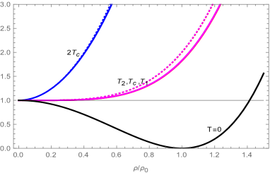
Figure 2: The effective thermal potential $V_{eff}=V_{T}-(\pi^{2}N/90)~{}NT^{4}$ (the solid lines) for $T=2T_{c},T_{2},T_{c},T_{1},$ and $0$. For comparison we plot the approximated potential shown in Eq. (12) in dashed lines. Here the unit of $V_{eff}$ is chosen to be $V_{0}=(\lambda/8)\rho_{0}^{4}=1$, and the horizontal line represents the $V_{eff}=V_{0}$. Notice that $V_{T}$ is almost indistinguishable at $T_{2},T_{c}$, and $T_{1}$.

The effective potential (with $\delta V_{T}=0$) has three local extrema at

$$\rho_{s}=0,$$

$$\rho_{\pm}(T)=\frac{C_{1}}{4\pi\lambda}~{}T\pm\sqrt{\Big{(}\frac{C_{1}}{4\pi\lambda}\Big{)}^{2}~{}T^{2}+\rho_{0}^{2}-\frac{2C_{2}}{\lambda}~{}T^{2}}.$$ (11)

The first extremum $\rho_{s}=0$ represents the Higgs vacuum of the symmetric (unbroken) phase, and the second extremum $\rho_{-}(T)$ represents the local maximum, and the third extremum $\rho_{+}(T)$ represent the local minimum Higgs vacuum of the broken phase. But notice that these two extrema $\rho_{\pm}$ appear only when $T$ becomes smaller than $T_{2}$

$$T_{2}=\frac{T_{1}}{\sqrt{1-\alpha^{2}}}\simeq 146.7~{}{\rm GeV},$$

$$T_{1}=\sqrt{\frac{\lambda}{2C_{2}}}~{}\rho_{0}\simeq 146.4~{}{\rm GeV},$$

$$\alpha=\frac{C_{1}}{4\pi\sqrt{2\lambda C_{2}}}\simeq 0.0662.$$ (12)

So above this temperature only $\rho_{s}=0$ becomes the true vacuum of the effective potential, and the electroweak symmetry remains unbroken.

At $T=T_{2}$ we have

$$\rho_{-}=\rho_{+}=(C_{1}/4\pi\lambda)~{}T_{2}\simeq 16.3~{}{\rm GeV},$$ (13)

but as temperature cools down below $T_{2}$ we have two local minima at $\rho_{s}$ and $\rho_{+}$ with $V_{T}(0)<V_{T}(\rho_{+})$, until $T$ reaches the critical temperature $T_{c}$ where $V_{T}(0)$ becomes equal to $V_{T}(\rho_{+})$,

$$T_{c}=\frac{T_{1}}{\sqrt{1-8\alpha^{2}/9}}\simeq 146.6~{}{\rm GeV},$$

$$\rho_{+}(T_{c})=\frac{C_{1}}{3\pi\lambda}~{}T_{c}\simeq 21.8~{}{\rm GeV}.$$ (14)

So $\rho_{s}=0$ remains the minimum of the effective potential for $T>T_{c}$. Notice that $T_{c}/\rho_{0}\simeq 0.6$ but $\rho_{+}/\rho_{0}\simeq 0.09$.

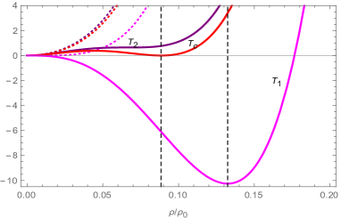
Figure 3: The amplified effective thermal potential for $T=T_{2},T_{c}$, and $T_{1}$. Here the vertical axis represents $V_{eff}-V_{0}$ in the unit $10^{-5}\times V_{0}$, and the vertical dashed lines indicate the positions of the local minima of the potentials. Here again the dashed lines represents the approximated potential (12).

Below this critical temperature $\rho_{+}$ becomes the true minimum of the effective potential, but $\rho_{s}=0$ remains a local (unstable) minimum till the temperature reaches $T_{1}$. But at $T=T_{c}$ the new vacuum bubbles start to nucleate at $\rho=\rho_{+}$, which takes over the unstable vacuum $\rho_{s}=0$ completely at $T=T_{1}$ when $\rho_{+}(T_{1})$ becomes around 32.6 GeV. From this point $\rho_{+}$ becomes the only (true) minimum, which approachs to the well-known Higgs vacuum $\rho_{0}$ at zero temperature.

The temperature dependence of the effective potential is schematically shown in Fig. 2. But since $V_{T}$ is almost indistinguishable at $T_{2},T_{c}$, and $T_{1}$, we have amplified it in Fig. 3. Notice that around the critical temperature $T\simeq T_{c}$ we have $\rho_{\pm}(T)\ll T$. This assures that the high temperature approximation of the effective potential (9) is trustable.

Fig. 3 tells that the phase transition from the local minimum from $\rho_{s}$ to the true minimum $\rho_{+}$ after $T=T_{c}$ is classically forbidden till $T$ reaches $T_{1}$, because the two minima are separated by an energy barrier. So during this period the transition must take place slowly through the quantum tunneling. Below this temperature the energy barrier disappears and we have free (fast) phase transition which generates a large latent heat. This means that the electroweak phase transition is of the first order.

In reality, however, Fig. 2 shows that the energy barrier is very small, which confirms that the phase transition is almost second order and . To see this notice first that from (14) we have $\rho_{+}(T_{c})/T_{c}\simeq 0.148$, which tells that the two degenerate vacua at $T=T_{c}$ are very close. And we can easily show that the height of the barrier between these vacua is extremely small,

$$\frac{V_{T_{c}}(\rho)|_{max}-V_{0}}{V_{0}}\simeq 3.83\times 10^{-6},~{}~{}~{}V_{0}=\frac{\lambda}{8}\rho_{0}^{4}.$$ (15)

Moreover, the barrier lasts only for short period since the temperature difference from $T_{c}$ to $T_{1}$ is very small, $\delta=(T_{c}-T_{1})/T_{c}\simeq 0.001$. From this we conclude that the electroweak phase transition is very mildly first order, in fact almost the second order.

Notice that it is the second term in (9) linear in $T$ which makes the electroweak phase transition first order. But this term does not change the effective potential much since it has a small coefficient compared to the third term (i.e., $C_{1}/12\pi\ll C_{2}/2$), and thus can be neglected. Neglecting this term we can approximate the effective potential to

$$V_{T}(\rho)\simeq V_{0}(\rho)+\frac{C_{2}}{2}\rho^{2}~{}T^{2}-\frac{\pi^{2}}{90}NT^{4}.$$ (16)

In this approximation we have $T_{c}=\sqrt{\lambda/2C_{2}}\rho_{0}=T_{2}=T_{1}=146.4$ GeV, so that $T_{c}$, $T_{1}$, and $T_{2}$ of the first order phase transition all become the same.

The effective potential (16) has only two minima, $\rho_{s}$ for $T>T_{c}$ and $\rho_{+}$ for $T<T_{c}$,

$$\rho_{s}=0,$$

$$\rho_{+}(T)=\sqrt{1-\Big{(}\frac{T}{T_{c}}\Big{)}^{2}}\rho_{0},$$ (17)

so that the phase transition becomes exactly the second order. For comparison this potential is plotted in Fig.2 and Fig. 3 in dashed lines.

However, there is one big difference between two effective potentials (9) and (16). In the first order phase transition the Higgs mass remains non-vanishing during the phase transition. From (9) we have

$$\bar{M}_{H}^{2}=\frac{d^{2}V_{eff}}{d\rho^{2}}\Big{|}_{\rho_{min}}$$

$$=\left\{\begin{array}[]{ll}\big{[}(T/T_{1})^{2}-1\big{]}M_{H}^{2}/2,&~{}~{}~{}T\geq T_{c},\\ \big{[}(\rho_{+}/\rho_{0})^{2}+1-(T/T_{1})^{2}\big{]}M_{H}^{2}/2,&~{}~{}~{}T<T_{c},\end{array}\right.$$ (20)

where $\bar{M}_{H}$ is the temperature-dependent Higgs mass. So $\bar{M}_{H}$ acquires its minimum value 5.53 GeV at $T=T_{c}$ and becomes 11.7 GeV at $T=T_{1}$, and approaches to the zero temperature value 125.7 GeV as the universe cools down. Of course, these cosmologically produced Higgs particles will quickly decay and disappear.

Similarly, the W-boson which was massless at high temperature becomes massive at $T=T_{c}$ when the Higgs field acquires the non-vanishing vacuum expectation value. So, as the Higgs vacuum $\rho=0$ starts to tunnel to $\rho=\rho_{+}$ at $T_{c}$, the W-boson starts to become massive toward the value $g\rho_{+}(T_{c})/2\simeq$ 7.1 GeV. And it acquires the mass 10.6 GeV at $T=T_{1}$, which approaches the well-known zero-temperature value 80.4 GeV at $T=0$.

On the other hand, in the second order phase transition we have from (16)

$$\bar{M}_{H}^{2}=\left\{\begin{array}[]{ll}\big{[}(T/T_{c})^{2}-1\big{]}M_{H}^{2}/2,&~{}~{}~{}T\geq T_{c},\\ \big{[}1-(T/T_{c})^{2}\big{]}M_{H}^{2},&~{}~{}~{}T<T_{c},\end{array}\right.$$ (23)

so that the Higgs mass becomes zero at $T_{c}$. This makes an important difference in the monopole production density, as we will see soon. The temperature-dependent Higgs and W-boson masses are shown in Fig. 4, where the blue and red curves represent the Higgs and W-boson masses, and the solid and dotted lines represent the first and second order and phase transitions.

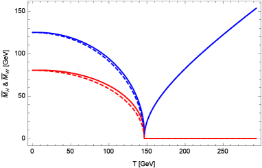
Figure 4: The temperature-dependent Higgs and W-boson masses. The blue and red curves represent the Higgs and W-boson masses, and the solid and dotted lines represent the masses in the first and second order and phase transitions.

IV Electroweak Monopole Production after Phase Transition

The production of magnetic monopole by the phase transition in early universe was discussed by Kibble and others, and later by Zurek who refined the Kibble’s estimate of the monopole density taking into account the dynamics of equilibrium processes kibble ; pres ; guth ; zurek . But before we discuss the cosmological electroweak monopole production, we briefly review the big bang cosmology in early universe.

The big bang cosmology is based on the cosmological principle which assumes that the universe is isotropic and homogeneous, and is described by the Robertson-Walker metric which implements this principle

$$ds^{2}=-dt^{2}+R^{2}(t)\Big{(}\frac{dr^{2}}{1-kr^{2}}$$

$$+r^{2}(d\theta^{2}+\sin^{2}\theta d\varphi^{2})\Big{)},$$ (24)

where $R$ is the scale factor and $k=\pm 1,~{}0$ represents the curvature (closed, open, and flat) of the universe. Coupled to the perfect fluid energy-momentum tensor $T_{\mu\nu}=(\varrho+p)\xi_{\mu}\xi_{\nu}+pg_{\mu\nu}$, the metric gives the familiar Friedmann equation

$$H^{2}+\frac{k}{R^{2}}=\frac{8\pi}{3}G_{N}\varrho,$$

$$\dot{\varrho}+3H(\varrho+p)=0,$$ (25)

where $H=\dot{R}/R$ is the Hubble parameter and $\varrho$, $p$, and $\xi_{\mu}$ are the density, pressure, and the 4-velocity of the perfect fluid. In the big bang cosmology one also assumes that the expansion is adiabatic,

$$\frac{d}{dt}(sR^{3})=0,$$ (26)

where $s$ is the entropy density of the universe.

The metric (24) tells that the coordinate distance the light (or a massless particle) which leaves $r=0$ at $t=0$ and arrives at $r$ after the time $t$ is

$$d(t)=\int_{t_{0}=0}^{t_{1}=t}\frac{dt^{\prime}}{R(t^{\prime})}=\int_{0}^{r}\frac{dr^{\prime}}{(1-kr^{\prime 2})^{1/2}},$$ (27)

so that the horizon distance of the universe at $t$ is given by

$$d_{H}(t)=R(t)\int_{0}^{t}\frac{dt^{\prime}}{R(t^{\prime})}=R(t)d(t).$$ (28)

Moreover, letting the light which leaves $\delta t_{0}$ later and travels the same coordinate distance arrive $\delta t_{1}$ later, we have

$$\frac{\delta t_{0}}{R(t_{0})}=\frac{\delta t_{1}}{R(t_{1})}.$$ (29)

From this we can define the “redshift” parameter $z$ by the ratio of the detected wavelength at $r_{1}$ to the emitted wavelength at $r=0$,

$$1+z=\frac{\lambda_{1}}{\lambda_{0}}=\frac{R(t_{1})}{R(t_{0})},$$ (30)

which provides us an important means to test the change of the scale factor $R(t)$ experimentally.

To solve the Friedmann equation we need to specify the equation of state of the matter. At high temperature the universe is in the radiation dominant era, and we may assume that the matter is made of ideal quantum gas of massless particles whose energy density $\varrho$ and entroty density $s$ are given by

$$\varrho=3p=\frac{\pi^{2}}{30}g_{*}(T)T^{4},~{}~{}~{}~{}~{}s=\frac{2\pi^{2}}{45}g_{s}(T)T^{3},$$

$$g_{*}=\sum_{\text{bosons}}g_{bi}\Big{(}\frac{T_{i}}{T}\Big{)}^{4}+\frac{7}{8}\sum_{\text{fermions}}g_{fi}\Big{(}\frac{T_{i}}{T}\Big{)}^{4},$$

$$g_{s}=\sum_{\text{bosons}}g_{bi}\Big{(}\frac{T_{i}}{T}\Big{)}^{3}+\frac{7}{8}\sum_{\text{fermions}}g_{fi}\Big{(}\frac{T_{i}}{T}\Big{)}^{3},$$ (31)

where $g_{i}$ and $T_{i}$ are the internal degrees and the temperature of the $i$-th relativistic particle.

From this we have (when the temperature is not near any mass threshold)

$$R=\Big{(}\frac{30E}{\pi^{2}g_{*}}\Big{)}^{1/4}~{}\frac{1}{T}=\Big{(}\frac{45S}{2\pi^{2}g_{s}}\Big{)}^{1/3}~{}\frac{1}{T},$$ (32)

where $E=\varrho R^{4}$ and $S=sR^{3}$ are the integration constants which represent the total energy and entropy of the universe.

With this (25) is written as

$$\Big{(}\frac{\dot{T}}{T}\Big{)}^{2}+\delta(T)T^{2}=\frac{4\pi^{3}}{45}G_{N}g_{*}T^{4},$$

$$\delta(T)=\frac{k}{R^{2}T^{2}}=k~{}\Big{(}\frac{\pi^{2}g_{*}}{30E}\Big{)}^{1/2}$$

$$=k~{}\Big{(}\frac{2\pi^{2}g_{s}}{45S}\Big{)}^{2/3}.$$ (33)

On the other hand, in the radiation dominant era, the curvature term $\delta(T)$ become negligible compared to the density term when $R$ becomes small, so that we may assume $k=0$. With this we can solve (33) and find

$$T^{2}\simeq\frac{Cm_{p}}{2t},$$ (34)

where $C=\sqrt{45/4\pi^{3}g_{*}(T)}$ and $m_{p}\simeq 1.2\times 10^{19}$ GeV is the Planck mass. This, with (32) gives

$$R(t)=\Big{(}\frac{30E}{\pi^{2}g_{*}}\Big{)}^{1/4}\sqrt{\frac{2t}{Cm_{p}}},$$

$$H=-\frac{\dot{T}}{T}\simeq\frac{T^{2}}{Cm_{p}}\simeq\frac{1}{2t},$$ (35)

This remains a good approximation for $T_{e}<T$, where $T_{e}\simeq 0.26~{}{\rm eV}$ is the temperature where the matter and radiation become equal.

From (25) we have

$$\Omega=\frac{\varrho}{\varrho_{c}}=1+\frac{k}{H^{2}R^{2}},~{}~{}~{}\varrho_{c}=\frac{3H^{2}}{8\pi G_{N}}.$$ (36)

Notice that $\Omega$ (as well as $\varrho$ and $\varrho_{c}$) is time-dependent. Since $H^{2}=(8\pi G_{N}/3)\varrho_{c}$, this can be written as

$$\Omega-1=\frac{k}{H^{2}R^{2}}\propto\frac{1}{T^{2}}.$$ (37)

This means that $k/H^{2}R^{2}$ must have been extremely small in the early universe. But this is very strange because this curvature term determines the fate of the universe in the later stage. This, of course, is the flatness problem.

From (35) we have the horizon distance given by

$$d_{H}(t)=R(t)\int_{0}^{t}\frac{dt^{\prime}}{R(t^{\prime})}=2t=\frac{Cm_{p}}{T^{2}}.$$ (38)

At the electroweak temperature all particles of the standard model contribute to $g_{*}$, so that we have $g_{*}\simeq 106.75$ and $C\simeq 0.058$. This tells that at $T=T_{c}$ the universe was roughly in $1.1\times 10^{-11}\sec$ after the big bang, and the horizon distance was about $d_{H}\simeq 1/H\simeq Cm_{p}/T_{c}^{2}\simeq 0.65~{}{\rm cm}$.

The cosmological principle presupposes that the universe is homogeneous. But obviously this does not mix well with the causality. To see this notice that the horizon size and the size of the universe fixed by the scale factor $R$ need not be the same. From (34) and (35) we have

$$\Big{(}\frac{d_{H}(T)}{R(T)}\Big{)}^{3}=\Big{(}\frac{\pi^{2}g_{*}}{30E}\Big{)}^{3/4}\Big{(}\frac{Cm_{p}}{T}\Big{)}^{3}\propto\frac{1}{T^{3}}.$$ (39)

So, normalizing $R$ by $d_{H}(T_{e})=R(T_{e})$, we can express the ratio of the horizon volume $V_{H}$ to the actual volume $V$ of the universe by (when $T_{e}<T$)

$$\Big{(}\frac{V_{H}(T)}{V(T)}\Big{)}^{3}=\Big{(}\frac{T_{e}}{T}\Big{)}^{3}.$$ (40)

So most of the universe which was visible and homogeneous at the matter-radiation eqality temperature were causally disconnected in the early universe. But it is difficult to understand how the causally disconnected universe became homogeneous at $T_{e}$. This is the essence of the horizon problem in the big bang cosmology.

Now we are ready to discuss the electroweak monopole production, or more precisely the monopole-antimonopole pair production, since they have to be crated in pairs. There have been many works on the monopole productions in the literature, but most of the discussions were on the grand unification monopole kibble ; pres ; guth ; zurek .

In general the monopole production mechanism depends on the type of the phase transition. There are two key factors which determine the initial monopole density, the time of the monopole formation and the correlation length of the phase transition at this time. And they depend on the type of phase transition.

In the second order phase transition the monopole formation is assumed to take place around the critical temperature. But in the first order phase transition the monopole formation is assumed to take place below the critical temperature, during the quantum tunneling through the vacuum bubble collisions. So the monopole production mechanism in two cases is totally different.

As we have pointed out, however, the electroweak phase transition is mildly the first order. This makes the electroweak monopole production more complicated and ; koba . So it is worth to discuss the electroweak monopole production in both the first order and second order phase transitions, and we discuss the two cases separately.

IV.1 Monopole production in the second order phase transition

In the phase transition the average distance between two topological defects is given by the correlation length, so that the initial monopole density is determined by the correlation length $\xi$ which is set by the Higgs mass, $\xi=1/\bar{M}_{H}$. But in the second order phase transition $\xi$ becomes infinite since the Higgs mass becomes zero at $T_{c}$. In this case the only parameter which sets the length scale at $T_{c}$ and can play the role of the correlation length is the horizon distance, and from the causality argument Kibble has proposed that the initial density of the monopole (and anti-monopole) must be bounded by the horizon distance kibble

$$\Big{(}\frac{n_{m}}{T^{3}}\Big{)}_{i}\gtrsim\Big{(}\frac{T_{c}}{Cm_{p}}\Big{)}^{3}\simeq 8.7\times 10^{-48}.$$ (41)

This Kibble bound has provided an important limit on the monopole density in the second order phase transition.

The phase transition, however, does not take place instantaneously but continuously, so that we have to incorporate the dynamics of equilibrium process. And the Kibble bound was refined by Zurek who took care of the relaxation time $\tau$ in the phase transition,

$$\tau=\frac{\tau_{0}}{|\varepsilon(T)|^{\mu}},~{}~{}~{}\xi=\frac{\xi_{0}}{|\varepsilon(T)|^{\nu}},$$

$$\varepsilon(T)=(T_{c}-T)/T_{c},$$ (42)

where $\varepsilon(T)$ is related with the quenching time scale $\tau_{Q}=t/\varepsilon$ which is related to $1/H(T_{c})$ in the cosmological context. Also the critical exponents $\mu$ and $\nu$ characterize the universality class of the transition, and $\tau_{0}$ and $\xi_{0}$ are dimensional parameters determined by the microphysics. In our case they are given by $\xi_{0}\approx\tau_{0}\sim 1/(\sqrt{\lambda}T_{c})$.

As the temperature approaches the critical value, $\tau$ becomes sufficiently longer and the process critically slows down. However, $\xi$ increase indefinitely but the propagation of small fluctuations is finite (limited by the speed of light). Therefore, there is a characteristic time $t_{*}$ when the correlation length freezes. From these the correlation length is given by $\xi(t_{*})=\xi_{0}|\tau_{0}/\tau_{Q}|^{\nu/(1+\mu)}$. The causality $\xi\leq c\tau$ implies $\nu\leq\mu$ and we will assume $\mu=\nu$ from now on.

With $\tau_{Q}\simeq H^{-1}(T_{c})=Cm_{p}/T_{c}^{2}$ the relic density of monopole following from the Zurek mechanism in the second order phase transition is expressed by

$$\Big{(}\frac{n_{m}}{T^{3}}\Big{)}_{i}\simeq\frac{g_{P}}{\xi^{3}(t_{*})T_{c}^{3}}$$

$$\simeq 0.02\times\Big{(}\frac{28.4T_{c}}{m_{p}}\Big{)}^{p},~{}~{}~{}~{}p={\frac{3\nu}{1+\nu}},$$ (43)

where $g_{P}$ is a geometrical factor of oder one-tenth. From this we can estimate the initial monopole production density

$$8.4\times 10^{-22}\lesssim\Big{(}\frac{n_{m}}{T^{3}}\Big{)}_{i}\lesssim 3.6\times 10^{-18},$$ (44)

where we have used critical exponent $\nu$ which is allowable in the field theory model, $0.5\leq\nu\leq 0.7$. The main difference between the Zurek result and the Kibble’s bound is the power $p$ of the $(T_{c}/m_{p})^{p}$ suppression factor. So, when $p$ is small, monopoles with relatively light mass can contribute to the dark matter substantially.

Actually there is a more realistic way to estimate the initial monopole density. To figure out the monopole density more accurately, the important thing to know is the time of the monopole formation. To find this, notice that the creation of the monopole requires the change of topology, in particular the appearance of zero points of the Higgs vacuum which become the seeds of the monopoles. Clearly these zero points do not appear instantaneously at the critical temperature, but are naturally induced by the thermal fluctuations of the Higgs field after the phase transition. This means that the monopoles do not appear at the critical temperature, but some time later.

To find the monopole production temperature, notice that, just below the critical temperature the Higgs field is still subject to large fluctuations which bring $\langle\rho\rangle$ back to zero. This is possible so long as

$$\xi^{3}\Delta F\leq T,$$ (45)

where $\xi(T)$ is the correlation length and $\Delta F(T)=V(\rho_{s})-V(\rho_{+})$ is the difference in free energy density between two phases with different symmetry. This is because the fluctuation energy should not exceed the thermal energy.

The temperature at which the equality holds in (45) is the Ginzberg temperature $T_{G}$. In the second order approximation (16) we have $\bar{M}_{H}^{2}=[1-(T/T_{c})^{2}]M_{H}^{2}$, so that the Ginzburg temperature is given by

$$T_{G}=\frac{T_{c}}{\sqrt{1+32\lambda^{2}/C_{2}}}\simeq 56.0~{}{\rm GeV},$$ (46)

which is lower than the critical temperature $T_{c}$. The correlation length $\xi_{G}$ which saturates the equality in (45) at the Ginzburg temperature is given by

$$\xi_{G}=\frac{\sqrt{1+32\lambda^{2}/C_{2}}}{8\lambda T_{c}}\simeq 1.7\times 10^{-16}~{}{\rm cm}.$$ (47)

This is well within the horizon distance.

Now, assuming that the monopoles are produced between $T_{c}$ and $T_{G}$ we may choose the correlation length $\xi_{i}$ which determines the initial monopole density and the corresponding monopole production temperature $T_{i}$ to be

$$\xi_{i}=\xi(T_{i})\simeq 2.2\times 10^{-16}~{}\text{cm},$$

$$~{}~{}~{}~{}T_{i}=\frac{T_{G}+T_{c}}{2}\simeq 101.2~{}\text{GeV}.$$ (48)

Now, let $g_{P}$ be the probability that one monopole is created inside a domain of size $\xi_{i}$. With this we find a new initial monopole density which can replace the Zurek bound,

$$\Big{(}\frac{n_{m}}{T^{3}}\Big{)}_{i}\simeq\frac{g_{P}}{\xi_{i}^{3}T_{i}^{3}}\simeq 7.1\times 10^{-2},$$ (49)

where we have assumed $g_{P}\simeq 0.1$. This is bigger than the Zurek bound (44) roughly by the factor $10^{16}$, which shows that the initial monopole density depends crucially on how to estimate it.

IV.2 Monopole production in the first order phase transition

The above pictures, however, may not properly describe the electroweak monopole production. This is because the Kibble and Zurek argument does not apply since the electroweak phase transition is the first order. When the phase transition is of the first order, the correlation length becomes finite because the Higgs mass becomes non-zero at the critical temperature. Moreover, the potential barrier between the symmetric and broken vacua modifies the Ginzburg temperature.

In the strongly first order phase transition, the symmetric vacuum becomes meta-stable below the critical temperature, and bubbles of broken phase will nucleate and expand. Within each bubble the Higgs field is correlated, but there is no correlation in Higgs field in difference bubbles. Thus when the bubbles collide, they can create the monopoles whose density is proportional to the density of bubbles. Since the expansion speed cannot exceed the speed of light, the size of a bubble is also limited by the horizon distance. So we have the following bound on the relic monopole abundance guth

$$\Big{(}\frac{n_{m}}{T^{3}}\Big{)}_{i}\gtrsim\Big{[}\frac{T_{c}}{Cm_{p}}\log\Big{(}\frac{Cm_{p}}{T_{c}}\Big{)}^{4}\Big{]}^{3}$$

$$\simeq 2.6\times 10^{-41}.$$ (50)

Notice that the logarithmic factor gives the enhanced monopole glut for the first order phase transition.

However, the electroweak phase transition is very mildly first order, so that the bubble formation and thus the monopole production by the bubble collisions becomes unimportant and negligible. Indeed, in the first order phase transition described by (9), we may neglect the tunneling of the potential barrier and assume that the monopole formation takes place after the phase transition is completed, between $T_{1}$ and the Ginzburg temperature. So we have to find the Ginzburg temperature first.

Unfortunately in this case the Ginzburg temperature can not be expressed in a simple form. But we can calculate $T_{G}$ numerically directly from the effective potential (9). With $\bar{M}_{H}^{2}=\lambda(\rho_{+}^{2}+\rho_{0}^{2})/2-C_{2}T^{2}$ we plot $\xi^{3}\Delta F$ and $T$ in red curve in Fig. 5. From this we find

$$T_{G}\simeq 57.6~{}\text{GeV},$$

$$\xi(T_{G})\simeq 1.7\times 10^{-16}~{}\text{cm},$$ (51)

which is almost identical to (46) and (47). This tells that, on the Ginzburg temperature and the correlation length, the second order approximation works quite well.

With this we may assume that the period of the monopole formation is between $T_{1}$ and $T_{G}$,

$$\bar{t}=t(T_{G})-t(T_{1})=\frac{Cm_{p}}{2T_{G}^{2}}-\frac{Cm_{p}}{2T_{1}^{2}}$$

$$=\frac{Cm_{p}}{2}\times\frac{T_{1}^{2}-T_{G}^{2}}{(T_{1}T_{G})^{2}}\simeq 6.0\times 10^{-11}~{}{\rm sec}.$$ (52)

And during this period the Higgs vacuum must fluctuate to zero to create the monopoles.

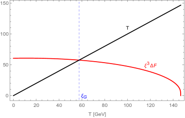
Figure 5: The determination of the Ginzburg temperature in the first order electroweak phase transition. Here the red and blue curve represents $\xi^{3}\Delta F$ and the black line represents $T$.

We can estimate the time scale of the fluctuation $\Delta t$ from the uncertainty principle $\Delta E\cdot\Delta t\simeq 1$, where $\Delta E$ is given by the Higgs vacuum $\rho_{+}$ around this time,

$$\Delta t\simeq\frac{1}{\Delta E}\simeq 5.0\times 10^{-27}~{}{\rm sec},$$

$$\Delta E\simeq\frac{\rho_{+}(T_{1})+\rho_{+}(T_{G})}{2}.$$ (53)

From this we can estimate the number of the fluctuations of the Higgs field,

$$N\simeq\frac{\bar{t}}{\Delta t}\simeq Cm_{p}\times\frac{(T_{1}^{2}-T_{G}^{2})(\rho_{+}(T_{1})+\rho_{+}(T_{G}))}{(T_{1}T_{G})^{2}}$$

$$\simeq 1.2\times 10^{16}.$$ (54)

This tells that there is ample time for the vacuum fluctuation of the Higgs field to produce the monopoles. From this we conclude that the dominant mechanism for the electroweak monopole production is not the bubble collisions during the phase transition but the quantum fluctuation of the Higgs vacuum after the phase transition.

From (51) we can estimate the initial density of the monopoles in the first order phase transition. Assuming that the monopoles are produced between $T_{1}$ and $T_{G}$, we have

$$\Big{(}\frac{n_{m}}{T^{3}}\Big{)}_{i}\simeq\frac{g_{P}}{\xi_{i}^{3}T_{i}^{3}}\simeq 9.1\times 10^{-4},$$

$$\xi_{i}=\frac{\xi(T_{1})+\xi(T_{G})}{2}\simeq 9.3\times 10^{-16}~{}\text{cm},$$

$$T_{i}=\frac{T_{1}+T_{G}}{2}\simeq 102.0~{}\text{GeV}.$$ (55)

Again this is a huge number compared with (44) or (50). Moreover, this is smaller than (49) by the factor $10^{-2}$, which tells that the second order approximation is not so trustable to estimate the monopole density. This is the main difference between our estimate and the old estimates.

Obviously, the monopole production consumes energy, so that we must know how much energy it consumes. If it consumes too much energy, it could cause us trouble. In fact, it is well known that in the grand unification the superheavy monopoles are produced too copiously that they force the universe supercool. Moreover, the mass of the remnant monopoles dominates the mass of all other matters by many orders of magnitude pres ; guth . Clearly, this is incompatible with the standard cosmology. So we have to check if the electroweak monopoles could cause a similar trouble.

To see how much energy we need to produce the electroweak monopoles, we can calculate the energy density of the monopoles from (55)

$$\varrho_{mo}(T_{i})=M_{m}(n_{m})_{i}\simeq 9.0\times 10^{-3}~{}T_{i}^{4}~{}\Big{(}\frac{M_{m}}{1~{}\text{TeV}}\Big{)},$$ (56)

where the mass of electroweak monopole is assumed to be around 1 TeV. This is because the monopole mass must be about 100 times bigger than the W-boson mass epjc15 ; ellis ; plb16 . This should be compared with the total energy density of the universe (31) at $T_{i}$

$$\frac{\varrho_{mo}(T_{i})}{\varrho(T_{i})}\simeq\frac{0.268}{\pi^{2}g_{*}(T_{i})}\Big{(}\frac{M_{m}}{1~{}\text{TeV}}\Big{)}$$

$$\simeq 2.5\times 10^{-4}\Big{(}\frac{M_{m}}{1~{}\text{TeV}}\Big{)}.$$ (57)

This tells that the universe need to consume only a tiny fraction (about $0.025~{}\%$) of the total energy to produce the monopoles. This is nice, because this assures that the monopole production does not alter the standard cosmology.

This is very important because, had the monopoles been produced too copiously, their energy density would have dominated the total energy density of the universe. In fact, this has been a major problem with the grand unification monopole kibble ; pres . The above result assures that the electroweak monopole has no such problem.

To see the importance of this observation, suppose $\xi_{i}$ in (55) were 10 times bigger. In this case $n_{m}$ would become 1000 times bigger, so that the universe would have to consume about a quarter of the total energy to produce the monopoles. This would have been a serious problem, because this might supercool the universe and could alter the standard cosmology.

In fact, we can say that even (55) is an overestimation. The reason is that, as we will see soon, the monopole-antimonopole capture radius becomes much bigger the correlation length $\xi_{i}$, so that most of the monopoles annihilate with the anti-monopoles as soon as they are produced. Moreover, this ahnnihilation continues very long time, till the universe cools down to about 29.5 MeV. This is basically because the monopoles couple strongly, i.e., magneticically.

Fortunately we do not have to worry about this overestimate of the initial monopole density. This is because, as we will see, the final density of the monopoles turns out to be rather insensitive to the initial monopole density.

V Density of Relic Electroweak Monopoles

Since the magnetic charge of the monopoles are topologically conserved, they are absolutely stable. So, once created, the monopoles do not decay. As we have pointed out, however, the initial monopole density changes. There are two factors which make this change, the Hubble expansion and the annihilation of monopole-antimonopole pairs, and the evolution of monopole (and anti-monopole) density $n_{m}$ is determined by the Boltzmann equation pres ; zel

$$\frac{dn_{m}}{dt}+3Hn_{m}=-\sigma n_{m}^{2}.$$ (58)

where $H$ and $\sigma$ are the Hubble parameter and the monopole-antimonopole annihilation cross section.

Obviously the Hubble expansion dilutes the monopole density, but the monopole-antimonopole annihilation also deflates the monopole density. And this annihilation process becomes very important for us to estimate the remnant monopole density at present universe.

To study this annihilation process, we have to find out the monopole-antimonopole annihilation cross section first. The annihilation is controlled by two competing forces, the thermal Brownian motion (random walk) in hot plasma of charged particles and the attraction between the monopoles and anti-monopoles. After the creation the monopoles diffuse in a hot plasma of relativistic charged particles by the Brownian motion with the mean free path $l_{\rm free}$,

$$l_{\rm free}=v_{T}t_{\rm free}\simeq{\sqrt{\frac{T}{M_{m}}}}\times\frac{M_{m}}{T\sum_{i}n_{i}\sigma_{i}}$$

$$=\frac{1}{BT}\sqrt{\frac{M_{m}}{T}},~{}~{}~{}~{}~{}B=\frac{1}{T}{\sum_{i}n_{i}\sigma_{i}},$$ (59)

where $v_{T}\simeq\sqrt{T/M_{m}}$ and $t_{\text{free}}$ are the thermal velocity and the mean free time of the monopoles, $n_{i}$ and $\sigma_{i}$ are the number density and the cross section of the $i$-th relativistic charged particles and the sum is the sum over all spin states pres .

Notice that here we have assumed that the Brownian motion of the monopoles is non-relativistic. This is justified by the fact that the monopoles produced (with the initial mass around $1~{}\text{TeV}$) can be treated as non-relativistic particles, even though the universe is still in the radiation dominant era.

With

$$n_{i}\simeq\frac{3\zeta(3)}{4\pi^{2}}T^{3},~{}~{}~{}\sigma_{i}\simeq\Big{(}\frac{g_{m}q_{i}}{4\pi}\Big{)}^{2}\frac{1}{T^{2}}=\Big{(}\frac{q_{i}}{e}\Big{)}^{2}\frac{1}{T^{2}},$$ (60)

we have

$$B\simeq\frac{3\zeta(3)}{4\pi^{2}}\sum_{i}\Big{(}\frac{q_{i}}{e}\Big{)}^{2}\simeq 0.09\times\sum_{i}\Big{(}\frac{q_{i}}{e}\Big{)}^{2},$$ (61)

where $q_{i}$ is the electric charge of the $i$-th particle and $\zeta(3)=1.202...$ is the Riemann zeta function. Since the charged particles in the plasma are the leptons and quarks, we may put $B\simeq 3$.

With this we can estimate the thermal velocity and the mean free length of the monopoles around the temperature $T_{i}$. With (55) we have $v_{T}\simeq 0.31\times(M_{m}/1~{}\text{TeV})^{-1/2}~{}c$ and $l_{\rm free}\simeq 2.0\times(M_{m}/1~{}\text{TeV})^{1/2}\times 10^{-16}~{}{\rm cm}$ at $T_{i}$.

Now, against the thermal random walk of the monopoles, we have the attractive Coulomb force between monopoles and anti-monopoles which makes them drift towards each other. The drift velocity $v_{d}$ of the monopole at a distance $r$ from the anti-monopole is given by vil

$$v_{d}\simeq\frac{1}{\alpha}\times\frac{1}{BT^{2}r^{2}}=\frac{\alpha_{m}}{BT^{2}r^{2}},$$ (62)

where $\alpha=e^{2}/4\pi$ is the electromagnetic fine structure constant and $\alpha_{m}$ is the monopole fine structure constant defined by $\alpha_{m}=g_{m}^{2}/4\pi$, where $g_{m}=4\pi/e$ is the magnetic charge of the monopole. Notice that $\alpha_{m}=1/\alpha$.

Clearly the drag force generated by the Coulomb attraction can dissipate enough energy for the monopoles to be captured by the nearby anti-monopoles. So we have the monopole-antimonopole bound states which quickly annihilate, when the mean free path becomes less than the capture radius

$$l_{\rm free}\leq r_{\text{capt}}=\frac{\alpha_{m}}{T},$$ (63)

where $r_{\text{capt}}$ is determined by the condition that the thermal energy is equal to the potential energy of the monopole-antimonopole pair. With (55) we have $r_{\text{capt}}\simeq 2.7\times 10^{-14}~{}\text{cm}$ at $T_{i}$. Notice that the capture radius is much bigger (about hundred times) than the mean free length and correlation length, which indicates that the monopoles are annihilated as soon as they are produced. This is a clear evidence that (55) could be an overestimation.

There is another strong evidence to support this observation. Notice that the drift velocity becomes $v_{d}(r=\xi_{i})\simeq 2~{}c$. This, of course, is an unrealistically large and impossible number. But this does tell that the Coulomb attraction between the monopoles and anti-monopoles is much more stronger than the thermal diffusion around $T_{i}$. This assures that the annihilation is much more important than the diffusion around $T_{i}$, so that as soon as they are created, they are annihilated. This shows that the initial monopole density (55) is indeed an overestimation.

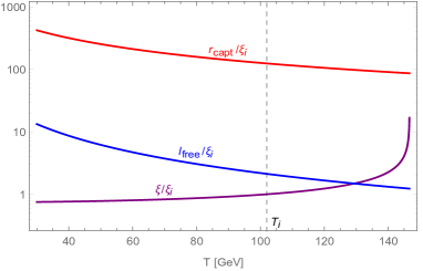
Figure 6: The relevant scales, $\xi$ in purple, $l_{\rm free}$ in blue, and $r_{\text{capt}}$ in red, against $T$. They are normalized by the correlation length $\xi_{i}$ at $T_{i}$. Here we set $M_{m}=5~{}{\rm TeV}$.

In Fig. 6 we plot the relevant scales $\xi$, $l_{\rm free}$, and $r_{\text{capt}}$ against $T$ for comparison. This confirms that the capture radius is much bigger than the mean free length and correlation length in a wide range of $T$, and reassures that the monopole-antimonopole annihilation is much more stronger than the monopole production.

Now, if we let the mean distance between the monopole and anti-monopole $r$ be $r\simeq n_{m}^{-1/3}$, the capture time is given by

$$t_{\text{capt}}\simeq\frac{r}{v_{d}}\simeq\alpha\times\frac{BT^{2}}{n_{m}}.$$ (64)

From this we have the monopole-antimonopole annihilation cross section

$$\sigma\simeq\frac{1}{t_{\text{capt}}n_{m}}\simeq\frac{\alpha_{m}}{BT^{2}}.$$ (65)

Notice that, with (55) we have $t_{\text{capt}}\simeq 1.6\times 10^{-19}~{}\text{sec}$ and $\sigma\simeq 1.7\times 10^{-30}~{}\text{cm}^{2}$ at $T_{i}$.

With this we can solve the Boltzmann equation (58). In term of $\tau=M_{m}/T$ the Boltzmann equation becomes

$$\frac{d}{d\tau}\Big{(}\frac{n_{m}}{T^{3}}\Big{)}=-\frac{\sigma T^{3}}{\tau H}\Big{(}\frac{n_{m}}{T^{3}}\Big{)}^{2}$$

$$=-\alpha_{m}\times\frac{Cm_{p}}{BM_{m}}\Big{(}\frac{n_{m}}{T^{3}}\Big{)}^{2}.$$ (66)

The analytic solution of the Boltzmann equation is well-known,

$$\frac{n_{m}}{T^{3}}=\frac{1}{A(\tau-\tau_{i})+B},$$

$$A=\alpha_{m}\times\frac{Cm_{p}}{BM_{m}},~{}~{}~{}B=\Big{(}\frac{n_{m}}{T^{3}}\Big{)}^{-1}_{i}.$$ (67)

Notice that when $\tau_{i}\ll\tau$, only the first term in the denominator becomes important. So the monopole density approaches to

$$\frac{n_{m}}{T^{3}}\rightarrow\alpha\times\frac{BT}{Cm_{p}},$$ (68)

regardless of the initial condition pres .

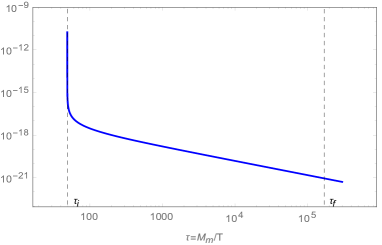
Figure 7: The evolution of the monopole density $n_{m}/T^{3}$ against $\tau=M_{m}/T$, which shows that most of the initial monopoles are quickly annihilated.

The evolution of the monopole density $n_{m}/T^{3}$ against $M_{m}/T$ is shown in Fig. 7, where we have put $M_{m}=5~{}{\rm TeV}$. This shows that most of the monopoles are annihilated as soon as created, after which the annihilation continues at a constant rate. Notice that here $B$ and the monopole mass $M_{m}$ are treated as constants, but strictly speaking they depends on time. So they should be understood as the mean values.

The diffusive capture process is effective only when $\ell_{\text{free}}<r_{\text{capt}}$, which determines the temperature $T_{f}$ below which the monopole-antimonopole annihilation ceases,

$$T_{f}\simeq\alpha^{2}\times\frac{M_{m}}{B^{2}}\simeq 5.9\times\Big{(}\frac{M_{m}}{1~{}\text{TeV}}\Big{)}~{}{\text{MeV}},$$ (69)

so that

$$\tau_{f}=\frac{M_{m}}{T_{f}}\simeq(\alpha_{m}B)^{2}\simeq 1.7\times 10^{5}.$$ (70)

With $M_{m}=5~{}{\rm TeV}$, we have $T_{f}\simeq 29.5~{}{\rm MeV}$, which is below the muon pair annihilation temperature. Actually, around this temperature $B$ becomes very small so that the capture radius becomes smaller. This is because the only charged particles remaining in the plasma are electrons and positrons. But the above analysis clearly shows that the annihilation continues very long time. The reason is basically the monopole-antimonopole attraction is much stronger than the electron-positron attraction.

Since $\tau_{i}\ll\tau_{f}$ the final density of the monopole at $T_{f}$ is independent of the initial density, and becomes

$$\Big{(}\frac{n_{m}}{T^{3}}\Big{)}_{f}\simeq\alpha^{3}\times\frac{M_{m}}{BCm_{p}}$$

$$\simeq 1.8\times 10^{-22}~{}\Big{(}\frac{M_{m}}{1~{}\text{TeV}}\Big{)},$$ (71)

where we have put $B\simeq 3$. Obviously this value is much lower than the initial density given by (55). This confirms that most of the monopoles produced initially are annihilated and diluted away.

As the temperature of universe cools down further, the annihilation process becomes unimportant, and the number of monopole within the comoving volume is conserved thereafter. Notice, however, that around $T_{f}$ the monopoles are still interacting with the electron pairs in the hot plasma. But eventually they decouple around $T_{d}\simeq 0.5~{}\text{MeV}$, when the electron pairs disappear and the monopole interaction rate becomes less than the Hubble expansion rate.

Assuming that the expansion is adiabatic, we have

$$\frac{n_{m}}{T^{3}}=1.8\times 10^{-22}\Big{(}\frac{M_{m}}{1~{}\text{TeV}}\Big{)}\Big{(}\frac{g_{s}(T)}{g_{s}(T_{f})}\Big{)},$$ (72)

so that the current number and energy density of monopole is given by

$$\Big{(}\frac{n_{m}}{T^{3}}\Big{)}_{0}=\Big{(}\frac{g_{s,0}}{g_{s,f}}\Big{)}\Big{(}\frac{n_{m}}{T^{3}}\Big{)}_{f},$$

$$\rho_{mo,0}=M_{m}n_{m,0}=M_{m}T_{0}^{3}\Big{(}\frac{g_{s,0}}{g_{s,f}}\Big{)}\Big{(}\frac{n_{m}}{T^{3}}\Big{)}_{f},$$ (73)

where $T_{0}=2.73~{}\text{K}=2.35\times 10^{-13}~{}\text{GeV}$ is the temperature of the universe today and $g_{s,f}$ is the effective number of degrees of freedom in entropy at $T_{f}$ shown in (31), which is equal to $g_{*}$ when all the relativistic species are in thermal equilibrium at the same temperature.

The current density parameter of monopole can be written

$$\Omega_{mo}~{}h^{2}=\frac{\rho_{mo,0}~{}h^{2}}{\rho_{c,0}}$$

$$=1.7\times 10^{11}\Big{(}\frac{3.94}{106.75}\Big{)}\Big{(}\frac{n_{m}}{T^{3}}\Big{)}_{f}\Big{(}\frac{M_{m}}{1\text{TeV}}\Big{)},$$ (74)

where $\rho_{c,0}={3H_{0}^{2}}/{8\pi G_{N}}$ is the current critical density of universe and $h\simeq 0.678$ is the scaled Hubble constant defined by $H_{0}/(100~{}\text{km}~{}\text{s}^{-1}~{}\text{Mpc}^{-1})$. From this and (72) we have

$$\Omega_{mo}~{}h^{2}\simeq 1.2\times 10^{-12}\times\Big{(}\frac{M_{m}}{1~{}\text{TeV}}\Big{)}^{2}.$$ (75)

With $h\simeq 0.678$ and $M_{m}\simeq$ 5 TeV, we have $\Omega_{mo}\simeq 6.53\times 10^{-11}$. This is about $1.31\times 10^{-9}$ of the baryon density, much less than the density of ${}^{3}{\rm He}$. This assures that the electroweak monopole cannot be a dark matter candidate.

In terms of the number density, this translates to about $6.1\times 10^{-20}~{}\text{cm}^{-3}$, or about $2.3\times 10^{-13}~{}n_{b}$, where $n_{b}\simeq 2.5\times 10^{-7}~{}\text{cm}^{-3}$ is the number density of the baryons. Intuitively, this means that there are roughly $6.6\times 10^{7}$ monopoles per every unit volume of the earth. This is a significant number, which suggests that there could be enough electroweak monopoles left over in the universe which we could detect.

VI Parker Bound on Monopole Density

Obviously the monopoles are accelerated in magnetic fields, in particular the intergalactic magnetic field. It is well known that the average strength of the galactic magnetic field $B$ is about $3\mu G\simeq 1.2\times 10^{-9}~{}\text{T}$. The energy gained by the monopole of charge $g_{m}=4\pi/e$ passing across the magnetic field $B$ of scale $L$ is

$$\Delta E=\frac{4\pi}{e}LB\simeq 1.2\times 10^{11}\times\Big{(}\frac{L}{10^{21}~{}{\rm cm}}\Big{)}~{}\text{GeV},$$ (76)

where $L$ is normalized to the typical coherence length of galactic magnetic field $L_{0}=300~{}\text{pc}\simeq 10^{21}~{}\text{cm}$. Traveling through the distance $L_{0}$, the monopole drains energy $\Delta E\simeq 10^{11}~{}\text{GeV}$ from the magnetic field and becomes ultra-relativistic pin . So, although the monopoles when decoupled around $29.5~{}\text{MeV}$ were non-relativistic, the remnant monopoles at present universe should be treated as relativistic.

Requiring that the rate of this energy loss in the galaxy is small compared to the time scale on which the galactic magnetic field can be regenerated, we can obtain the upper bound on the flux of the monopoles (with mass $M_{m}\leq 10^{17}~{}\text{GeV}$),

$$F\leq 10^{-15}~{}\text{cm}^{-2}\text{sec}^{-1}\text{sr}^{-1}.$$ (77)

This is the Parker bound parker .

The Parker bound sets a limit on the monopole density in the universe. The monopoles with velocity $v_{m}$ uniformly distributed throughout the universe generate the monopole flux turner

$$F\simeq\frac{v_{m}}{4\pi}n_{m,0}=\frac{v_{m}}{4\pi}\Big{(}\frac{\rho_{c,0}}{h^{2}M_{m}}\Big{)}\Omega_{mo}h^{2}$$

$$\simeq 2.3\times 10^{-2}~{}\Omega_{mo}h^{2}~{}\Big{(}\frac{v_{m}}{10^{-3}c}\Big{)}$$

$$\times\Big{(}\frac{1~{}{\rm TeV}}{M_{m}}\Big{)}~{}\text{cm}^{-2}\text{sec}^{-1}\text{sr}^{-1},$$ (78)

where $v_{m}$ is expressed in terms of the average virial velocity of the galaxy $10^{-3}c$. This, with (77), requires

$$\Omega_{mo}h^{2}\lesssim 4.3\times 10^{-14}\Big{(}\frac{10^{-3}c}{v_{m}}\Big{)}\times\Big{(}\frac{M_{m}}{1~{}{\rm TeV}}\Big{)}.$$ (79)

This set a stringent limit on the density for the relativistic ($v_{m}\simeq c=1$) electroweak monopoles. This causes us a serious trouble, because our estimate of the density parameter (75) is roughly $10^{5}$ times bigger than this limit.

We could think of possible ways to circumvent this trouble. First of all, we might suppose that the limit (79) is not trustable. Obviously this is an approximation. For example, the monopoles in the galactic magnetic field, when accelerated near the velocity of light, will make the Chrenkov radiation and will slow down to a limiting velocity considerably less than the velocity of light.

But a more realistic explanation could be that most of the electroweak monopoles in the universe are actually buried inside the galactic cores. This is quite possible, because the electroweak monopoles become the natural source for the premodial black holes and the structure formation. Certainly, as the heaviest stable particles, they could easily cause the density pertubation and become the seeds for the large scale structures in the universe.

Another possibility is that many of the electroweak monopoles are captured inside stellar objects when they hit (large) stellar objects, because they have a large capture cross section due to the magnetic interaction. In fact a relativistic electroweak monopole with mass 5 TeV is expected to travel less than 10 m in Aluminum before they are trapped bolo . So the electroweak monopoles coming to the earth loose most of the energy passing through the earth atmospheric sphere and become non-relativistic, and could easily be trapped near the earth surface. In fact we may conjecture that these trapped monopoles (and buried in large scale structures) could have been the very source of the intergalactic magnetic field.

More importantly, this strongly suggests that the stellar objects could have filtered out and diluted the density of the monopoles in the universe greatly, so that the remnant monopole density at present universe might have become much smaller than (55). So at this moment it is not clear whether our result is in contradiction with the Parker bound.

VII Discussions

In this paper we have studied the cosmic production and evolution of the electroweak monopole, and estimated the remnant monopole density in the present universe. Our analysis confirms that, although the electroweak phase transition is of the first order, it is very mildly first order. So the monopole production mechanism is not the vacuum bubble collisions during the phase transition but the thermal fluctuations of the Higgs field after the phase transition, which plant the seed of the monopoles.

Our result shows that the electroweak monopoles are produced when the temperature of the universe was around $100~{}{\rm GeV}$ (or about $10^{-11}~{}{\rm sec}$ after the big bang). And initially the monopoles are produced copiously, perhaps a bit too copiously to be realistic. But most of them are annihilated as soon as created, and this annihilation continues for a long time until the universe cools down to around 39.5 MeV, even after the muon pair annihilation. And eventually they decouple from the other matters at around $0.5~{}\text{MeV}$, when the electron pairs annihilate and the monopole interaction rate becomes less than the Hubble expansion rate.

Because of this the electroweak monopole density become very small, $\Omega_{mo}\simeq 6.3\times 10^{-11}$, in the present universe. This tells that, unlike the grand unification monopole, the electroweak monopole can not overclose the universe. As importantly, this assures that the production of the electroweak monopole does not alter the standard cosmology in any significant way, and exclude the possibility the electroweak monopole to be a candidate of the dark matter.

On the other hand, this means that there are enough monopoles left over, roughly $6.6\times 10^{7}$ monopoles per every unit volume of the earth in the present universe. This strongly indicates that experimentally there are enough remnant monopoles that we should be able to detect without much difficulty.

However, we should to keep in mind the possibility that the actual density of the remnant monopoles could be much less than this. This is because many of them could have been buried in the the large scale structures of the universe and/or filtered out by stellar objects. In fact, the actual monopole density could be smaller by the factor $10^{-5}$, or about $10^{3}$ per every unit volume of the earth, as the Parker bound indicates.

Our result could provide useful informations for the monopole detection experiments. The recently upgraded 13 TeV LHC at CERN might have finally reached the threshold energy to produce just one electroweak monopole-antimonopole pair. In this case MoEDAL has a best chance to detect the monopole. However, it is not clear if LHC could actually produce the monopole pair. This is an important issue, because if the monopole mass is larger than 6.5 TeV, LHC is not supposed to be able to produce the monopole.

Another issue is the monopole production mechanism at LHC. It has generally been believed that LHC could produce the monopole pair by Drell-Yan process ($p\bar{p}\rightarrow\gamma\rightarrow M\bar{M}$) and/or photon fusion process ($p\bar{p}\rightarrow p\bar{p}+\gamma\gamma\rightarrow p\bar{p}+M\bar{M}$) dypf . This would be the case if we treat the monopole as a point particle. But since the monopole is a topological particle, it is not clear if this is correct. Even if this picture is correct, LHC certainly need the change of topology to create the monopole pair, and we have to explain how LHC can achieve this during the collision.

Our analysis suggests that the cosimc monopole production mechanism should apply equally well to LHC. In other words, LHC could produce the monopole pair when the colliding beam core cools down from the maximum temperature 13 TeV in the symmetric phase to the electroweak phase around 100 GeV. At this temperature the thermal fluctuation of the Higgs field makes the monopole seeds, the baby monopoles, of mass around 1 TeV. This is several times less than the monopole mass at zero temperature which is expected to be several TeV. This strongly implies that the energy constraint of the LHC on the production of the electroweak monopole may not be so strong obstacle as we have thought.

To produce the monopole-antimonopole pair, however, our analysis tells that LHC should satisfy two more conditions. First, it should generate the hot plasma of the beam core of the size at least as big as the initial correlation length $\xi_{i}\simeq 10^{-15}~{}\text{cm}$. Second, this beam core should last at least ten times longer than $10^{-26}~{}\text{sec}$ to allow enough fluctuations for the Higgs vacuum to plant the monopole seed.

Fortunately, the size of the beam core at LHC has been measured to be about $0.03~{}\text{cm}$ and lasts for about $10^{-12}~{}\text{sec}$, long enough for the Higgs field to allow more than enough thermal flucuations lhc . This strongly implies that there is a good chance that LHC could actually produce one monopole-antimonopole pair, which MoEDAL could detect.

For the other experiments searching for the remnant monopoles in the universe, in particular for IceCube, ANTARES, and Auger, an important thing is to know the characteristic features of the remnant monopoles icecube ; antares ; auger . Although the electroweak monopoles were non-relativistic when they decoupled, the intergalactic magnetic field makes them highly relativistic at present universe. On the other hand, they loose most of the energy passing through the earth atmospheric sphere, so that near the earth surface they become non-relativistic again. So on earth these experiments should look for the non-relativistic monopole coming from the sky, which has mass around 4 to 10 TeV and magnetic charge $4\pi/e$.

In principle these experiments have the ability to detect the monopoles, but there is one catch here. These detectors (except Auger) are located underground. This could cause a problem, because the non-relativistic remnant monopoles may be trapped before they reach the detector. For example, IceCube is located under the 2 km thick iceberg, which the remnant monopoles may not be able to penetrate. If so, it would be very difficult for IceCube to detect the monopole. In fact this could be a main reason why IceCube could not find it. This suggests that a best way to detect the remnant monopole is to install the detector at high altitude. So these experiments have to find a way to circumbent this problem to detect the remnant monopoles.

Although the remnant electroweak monopoles in the present universe are insignificant, they have important physical implications. As we have speculated, they could have been the seed of the large scale structures in the universe. Indeed the electroweak monopoles with mass about $10^{4}$ times heavier than the proton, could easily generate the density perturbation and become an excellent candidate for the seed of the large scale structures in the universe. Moreover, as the heaviest relativistic magnetically charged particles in the universe, they become the source of ultra-high energy cosmic rays. Furthermore, they could play an important role in the electroweak baryogenesis. Clearly this is a very interesting possibility need to be studied further.

But the most important point of the electroweak monopole is that it must exist. This makes the detection of the electroweak monopole the final (topological) test of the standard model. In spite of huge efforts, however, the monopole detection so far has not been successful. There could be two reasons for this. First, many of these experiments were the blind seraches in the dark room, with few theoretical leads. Second, many were looking for different type of monopoles, in particular the grand unification monopole.

So, aiming at the electroweak monopole which has the unique characteristic features, we could enhance the probability to detect the monopole greatly. We hope that our analysis in this paper could help confirm the existence of the electroweak monopole.

ACKNOWLEDGMENT

The authors thank James Pinfold for the careful reading of the manuscript and valuable advice to improve the paper. The work is supported in part by the National Research Foundation of Korea funded by the Ministry of Education (Grants 2015-R1D1A1A0-1057578 and 2015-R1D1A1A0-1059407), and by Konkuk University.

References

- (1) P.A.M. Dirac, Proc. Roy. Soc. London, A133, 60 (1931); Phys. Rev. 74, 817 (1948).
- (2) T.T. Wu and C.N. Yang, in Properties of Matter under Unusual Conditions, edited by H. Mark and S. Fernbach (Interscience, New York) 1969; Phys. Rev. D12, 3845 (1975); Y.M. Cho, Phys. Rev. Lett. 44, 1115 (1980); Phys. Lett. B115, 125 (1982).
- (3) G. ’t Hooft, Nucl. Phys. B79, 276 (1974); A.M. Polyakov, JETP Lett. 20, 194 (1974); M. Prasad and C. Sommerfield, Phys. Rev. Lett. 35, 760 (1975).
- (4) C. Dokos and T. Tomaras, Phys. Rev. D21, 2940 (1980).
- (5) Y.M. Cho and D. Maison, Phys. Lett. B391, 360 (1997).
- (6) Yisong Yang, Proc. Roy. Soc. London, A454, 155 (1998); Yisong Yang, Solitons in Field Theory and Nonlinear Analysis (Springer Monographs in Mathematics), p. 322 (Springer-Verlag) 2001.
- (7) Kyoungtae Kimm, J.H. Yoon, and Y.M. Cho, Eur. Phys. J. C75, 67 (2015); Kyoungtae Kimm, J.H. Yoon, S.H. Oh, and Y.M. Cho, Mod. Phys. Lett. A31, 1650053 (2016).
- (8) J. Ellis, N.E. Mavromatos, and T. You, Phys. Lett B756, 29, (2016).
- (9) Y.M. Cho, Kyoungtae Kimm, J.H. Yoon, Phys. Lett. B761, 203 (2016).
- (10) B. Acharya et al. (MoEDAL Collaboration), Phys. Rev. Lett. 118, 061801 (2017).
- (11) B. Acharya et al. (MoEDAL Collaboration), JHEP 1608, 067 (2016); Int. J. Mod. Phys. A29, 1430050 (2014); Y.M. Cho and J. Pinfold, Snowmass white paper, arXiv: hep-ph/1307.8390.
- (12) R. Abbasi et al. (IceCube Collaboration) Phys. Rev. D87, 022001 (2013); M. Aartsen et al. (IceCube Collaboration), Eur. Phys. J. C74, 2938 (2014).
- (13) S. Adrián-Martinez et al. (ANTARES Collaboration), Astropart. Phys. 35, 634 (2012).
- (14) A. Aab et al. (Pierre Auger Collaboration) Phys. Rev. D94, 082002 (2016).
- (15) T.W.B. Kibble, J. Phys. A9 1387 (1976).
- (16) J.P. Preskill, Phys. Rev. Lett. 43, 1365 (1979).
- (17) A. Guth and E. Weinberg, Nucl. Phys. B212, 321 (1983).
- (18) W.H. Zurek, Phys. Rep. 276 177 (1996).
- (19) A. Guth, Phys. Rev. D23, 347 (1981); A. Linde, Phys. Lett. B108 389 (1982).
- (20) D. Krizhnits and A. Linde, Phys. Lett. B42, 471 (1972); C. Bernard, Phys. Rev. D9, 3312 (1974); L. Dolan and R. Jakiw, Phys. Rev. D9, 3320 (1974); S. Weinberg, Phys. Rev. D9, 3357 (1974).
- (21) Y.B. Zel’dovich and M.Yu. Khlopov, Phys. Lett. 79B, 239 (1978); P. Adams,V. Canuto, and H.Y. Chiu, Phys. Lett. 61B, 397 (1976).
- (22) G. Anderson and L. Hall, Phys. Rev. D45, 2685 (1992); M. Dine, R. Leigh, P Huet, A. Linde, and D. Linde, Phys. Rev. D46, 550 (1992).
- (23) S. Arunasalam and A. Kobahhidze, arXiv: hep-ph/1702.04068 (2017).
- (24) S. Coleman, Aspects of Symmetry (Cambridge Univ. Press, 1985); T. Vachaspati and M. Barriola, Phys. Rev. Lett. 69, 1867 (1992).
- (25) A. Vilenkin and E. Shellard, Cosmic Strings and other Topological Defects (Cambridge University Press) 1994.
- (26) S. Burdin, M. Fairbaim, P. Mermod, D. Milstead, J. Pinfold, T. Sloan, and W. Taylor, Phys. Rep. 582, 1 (2015).
- (27) E.N. Parker, Astrophys. J. 160, 383 (1970).
- (28) M.S. Turner, E.N. Parker, and T.J. Bogdan, Phys. Rev. D26, 1296 (1982); F.C. Adams, M. Fatuzzo, K. Freese, G. Tarlé, R. Watkins, and M.S. Turner, Phys. Rev. Lett. 70, 2511(1993).
- (29) S. Cecchini, L. Patrizii, Z. Sahnoun, G. Sirri, and V. Togo, arXiv: hep-ph/1606.01220.
- (30) T. Dougall and S. Wick, Euro. Phys. J. A39, 213 (2009); L. Epele, H. Fanchiotti, C. Cannl, V. Mitsou, and V. Vento, Euro. Phys. J. Plus 127, 60 (2012).
- (31) Redaelli, Stefano, et al., FERMILAB-CONF-15-135-AD-APC, 2015.