Conservation laws, vertex corrections, and screening in Raman spectroscopy

Abstract

We present a microscopic theory for the Raman response of a clean multiband superconductor, with emphasis on the effects of vertex corrections and long-range Coulomb interaction. The measured Raman intensity, $R(\Omega)$, is proportional to the imaginary part of the fully renormalized particle-hole correlator with Raman form-factors $\gamma({\vec{k}})$. In a BCS superconductor, a bare Raman bubble is non-zero for any $\gamma({\vec{k}})$ and diverges at $\Omega=2\Delta+0$, where $\Delta$ is the largest gap along the Fermi surface. However, for $\gamma({\vec{k}})=$ const, the full $R(\Omega)$ is expected to vanish due to particle number conservation. It was long thought that this vanishing is due to the singular screening by long-range Coulomb interaction. We show diagrammatically that this vanishing actually holds due to vertex corrections from the same short-range interaction that gives rise to superconductivity. We further argue that long-range Coulomb interaction does not affect the Raman signal for any $\gamma({\vec{k}})$. We argue that vertex corrections eliminate the divergence at $2\Delta$ and replace it with a maximum at a somewhat larger frequency. We also argue that vertex corrections give rise to sharp peaks in $R(\Omega)$ at $\Omega<2\Delta$, when $\Omega$ coincides with the frequency of one of collective modes in a superconductor, e.g, Leggett and Bardasis-Schrieffer modes in the particle-particle channel , and an excitonic mode in the particle-hole channel.

I Introduction

Raman spectroscopy is a useful tool to probe the electronic properties of a correlated metal. It is specifically important for superconductors (SC) because it can probe not only particle-hole excitations, but also particle-particle fluctuations of the condensate, making it an extremely valuable probe to study collective excitations in a SC, both in the dominant and in the subdominant pairing channel. Raman scattering can probe fluctuations in any scattering geometry, regardless of the symmetry of the SC state. This unique ability of Raman spectroscopy is due to the fact that a given geometry can be selected by choosing the polarizations of the incoming and the scattered light relative to the crystallographic axes.Sastry1990 ; Deveaux

If the energy of the incident and scattered light is smaller than the gaps between the bands which cross the Fermi level and those which don’t, the would be resonant scattering between these two types of bands is absent, and the Raman intensity, $R(\Omega)$, can be evaluated in the non-resonant approximation, where it is proportional to the imaginary part of the fully renormalized correlation function of modulated densities of fermions from the bands which cross the Fermi level: $R(\Omega)\propto{\rm Im}\left[\sum_{{\vec{k}}}\langle\rho^{R}({\vec{k}},0)\rho^{R}({\vec{k}},\Omega)\rangle\right]$, where $\rho^{R}({\vec{k}})=\sum_{a}\rho^{R}_{a}({\vec{k}})$, $a$ labels the bands, and $\rho_{R}^{a}({\vec{k}})=\gamma^{a}({\vec{k}})c^{\dagger}_{a}({\vec{k}})c_{a}({\vec{k}})$. The form-factor $\gamma^{a}({\vec{k}})$ (also called the Raman vertex) is expressed in terms of particular components of the effective mass tensorDeveaux which depends on the polarization of the incoming and outgoing light. In the absence of a sizable overlap between density operators with the same ${\vec{k}}$ from different bands, $R(\Omega)$ can be further approximated by $\sum_{{\vec{k}},a}\langle\rho_{R}^{a}({\vec{k}},0)\rho_{R}^{a}({\vec{k}},\Omega)\rangle$.

Non-resonant Raman spectroscopy has been used extensively to extract the pairing gap $\Delta$ and analyze various collective modes in the particle-particle channel, like the LeggettLeggett and Bardasis Schrieffer(BS) modes. BardasisSchrieffer61 ; vaks ; zawadowskii The former corresponds to fluctuations of the relative phases of the condensed order parameters in a multiband superconductor, and the latter corresponds to gapped fluctuations of an un-condensed order parameter in a subleading attractive pairing channel (e.g. fluctuations of a $d-$wave order parameter in an $s-$wave SC if both $s-$ wave and $d-$wave channels are attractive, but attraction in the $d-$wave is weaker than that in the s-wave channel). The Leggett mode has been reported to be observed in Raman experiments on MgB₂  MGB2 ; kkklein in the A_1g scattering geometry. BS modes have not been observed in conventional SCs, presumably because the competing attractive non $s$-wave pairing channels are too weak. However, a BS mode was predicted in Fe-based SC, because in many of these materials the $d-$wave channel is attractive, and the attraction is sometimes as strong as the one in the $s-$wave channel.rev1 ; rev2 Raman experiments on hole doped Ba_1-xK_xFe₂As₂ Hackl12 ; Hackl14 and electron-doped NaFe_1-xCo_xAsBlumberg14 have reported features in the d-wave (B_1g) channel, consistent with a BS mode.

There are also two other collective modes in a superconductor. One is a Boguliubov-Anderson-Goldstone (BAG) mode of phase fluctuations, associated with spontaneously broken U(1) symmetry (fluctuations of the overall phase of different condensates in case of a multiband SC). The BAG mode is massless in a charge-neutral superfluid, but becomes a plasmon in a charged superconductor due to long-range Coulomb interaction. The other is an amplitude mode of a condensateL0 ; L1 ; L2 , often called Higgs mode by analogy with the massive boson mode in the Standard Model of particle physics. The amplitude and the phase modes decouple in a BCS superconductor in the absence of time reversal symmetry breaking.spisLegett2 ; spisLegget1 ; SM_AVC ; Benfatto Neither of these modes is, however, Raman-active, unless special conditions are met. The phase mode only contributes to the Raman intensity with a weight $\propto q^{2}$, where $q$ is the momentum at which the Raman signal is measured. In Raman experiments, the momentum $q$ is smaller by $v_{F}/c$ than a typical fermionic momentum $k\sim\Omega/v_{F}$. Accordingly, the spectral weight of the phase mode contribution to the Raman intensity is very small. The amplitude does not directly couple to $\rho_{R}$, and appears in the Raman response only when there is an interaction with other collective modes like phonons or magnons,Zwerger and/or when superconductivity emerges out of a pre-existing charge-density-wave state.L0 ; Little In this work we do not take phonons or magnons into consideration, and do not assume pre-existing density-wave order.

The theory of non-resonant Raman response in superconductors has a long history.ABGenkin ; Klein ; ABF ; zawadowskii ; griffin ; devereaux For a superconductor with a minimal gap $\Delta$, the Raman intensity $R(\Omega)$, computed within BCS theory, as the imaginary part of a bare particle-hole bubble with $\gamma^{a}({\vec{k}})$ in the vertices, is non-zero at $\Omega>2\Delta$ and has an edge singularity at $\Omega=2\Delta+0$ in all scattering geometries. This holds even if $\gamma^{a}({\vec{k}})$ is a constant. For a nodal superconductor, $R(\Omega)$ is non-zero for all frequencies and has a singularity at $\Omega=2\Delta_{\rm max}$, where $\Delta_{\rm max}$ is the maximum gap. In this respect, the behavior of a bare particle-hole bubble in a superconductor differs from that in the normal state, where the free-fermion particle-hole bubble vanishes in the limit when $\Omega$ is finite and $q\to 0$ (more specifically, when $\Omega\gg v_{F}q$). This vanishing in the normal state is related to particle number conservation and holds for any $\gamma^{a}({\vec{k}})$ because for free fermions each $n_{k}$ in $N=\sum_{{\vec{k}}}n_{{\vec{k}}}$ is separately conserved. A non-zero value of this bubble in a superconductor is the consequence of the fact that a BCS Hamiltonian formally does not conserve the number of fermions due to the presence of $c^{\dagger}_{k}c^{\dagger}_{-k}$ and $c_{k}c_{-k}$ terms.

Several groups argued dev_2 ; Deveaux ; Girsh ; PeterBoyd that $R(\Omega)$ in one-band superconductor indeed vanishes for $\gamma({\vec{k}})=$ const, once one adds to BCS Hamiltonian the 4-fermion interaction term describing long-range Coulomb interaction $V_{C}({\vec{q}})$. This interaction renormalizes $R(\Omega)$ by adding RPA-type series of particle-hole bubbles coupled by $V_{C}({\vec{q}})$ [the upper line in Fig. 1]. In a two-band superconductor, a similar consideration Girsh yielded a partial reduction of $R(\Omega)$ when $\gamma({\vec{k}})$ are momentum-independent, but not equal for the two bands.

This point of view has been challenged recently by Cea and Benfatto Lara . They used gauge-invariant effective action approach and computed the Raman response of a one-band and two-band $s-$wave SC in A_1g geometry. They argued that the total number of fermions, including fermions in the condensate, is a conserved quantity. As the result, when $\gamma^{a}({\vec{k}})$ is a constant, independent of $a$, the fully dressed $R(\Omega)$ must vanish already before one includes the renormalizations due to Coulomb interaction, because in this case Raman susceptibility coincides with the density susceptibility, and the latter must vanish at $q=0$ and finite $\Omega$ due to conservation of the total number of particles (or, equivalently, of the total charge).

In this communication we analyze Raman response of one-band and multi-band superconductors with various pairing symmetry using a direct diagrammatic approach. We argue that the full gauge-invariant diagrammatic analysis of Raman intensity in a superconductor necessarily includes the processes which renormalize a given particle-hole bubble (the lower line in Fig. 1). We show, in agreement with Ref. [Lara, ], that these renormalizations give rise to the vanishing of $R(\Omega)$ for $\gamma({\vec{k}})=$ const even before one adds long-range Coulomb interaction. Moreover, we argue that long-range Coulomb interaction is completely irrelevant for Raman scattering at vanishing $q$ and finite $\Omega$, because RPA renormalizations between dressed bubbles only give contributions to $R(\Omega)$ which scale as at least as $q^{2}$.

We treat a superconductor within a weak coupling approach. In this limit, the fermionic self-energy is irrelevant, and essential renormalizations within a particle-hole bubble come from the ladder series of vertex corrections. We categorize these vertex corrections into two categories – particle-hole and particle-particle contributions. The first ones involve pairs of fermionic Green’s functions with opposite direction of arrows, the second ones involve pairs of fermionic Green’s functions with the same direction of arrows, as shown in Fig. 2. These combinations appear in a superconductor once a particle-hole pair, which couples to the light, gets converted into a particle-particle pair via a process which propagates as one normal and one anomalous Green’s function. We show that the conservation of the total number of particles guarantees certain cancellations between the bare bubble and the renormalizations from vertex corrections in the particle-particle channel. As a result:

• For a constant $\gamma^{a}({{\vec{k}}})$, $R(\Omega)$ for a one-band superconductor vanishes once one includes vertex corrections in the particle-particle channel. This holds even if we additionally include vertex corrections in the particle-hole channel (see also Ref. [Lara, ]).

• For a momentum-dependent $\gamma^{a}({{\vec{k}}})$, $R(\Omega)$ is non-zero, but the “$2\Delta$” edge singularity is removed and replaced by a maximum at an energy above $2\Delta$. This holds for isotropic or anisotropic systems and all scattering geometries.

• In a multi-band superconductor, $R(\Omega)$ vanishes due to vertex corrections in the particle-particle channel, when $\gamma^{a}({{\vec{k}}})$ has the same constant value for all bands (see also Ref. [Lara, ]).

• When $\gamma^{a}({{\vec{k}}})$ is either momentum-dependent, or has different constant values for different bands, $R(\Omega)$ is non-zero, but the “$2\Delta$” edge singularity is again eliminated and replaced by a maximum at a frequency above $2\Delta$.

• In both one-band and multi-band nodeless superconductors, $R(\Omega)$ generally vanishes below twice the minimum gap $2\Delta^{a}$, but under proper conditions may have $\delta-$function contributions at $\Omega<2\Delta^{a}$ from Leggett and BS-type modes in the particle-particle channel, and from excitonic modes in the particle-hole channel. In nodal superconductors, $R(\Omega)$ is finite at all frequencies and the contributions from collective modes appear as resonance peaks with a finite width.

• The Coulomb interaction does not affect $R(\Omega)$ at $\Omega\gg v_{F}q\rightarrow 0$. For non s-wave scattering geometry, this holds due to symmetry reasons and is well-known. We argue that this also holds for $s-$wave scattering geometry in one- and multi-band systems, and in isotropic and lattice systems (where the $s-$wave Raman vertex $\gamma^{a}_{{\vec{k}}}$ is momentum-dependent and the Raman bubble is different from a density-density bubble).

Vertex corrections inside a particle-hole bubble have been analyzed in the past. The Raman response in a 1-band SC was worked out in Ref. [Klein, ]. Our formulas fully agree with the ones in their work, although we interpret the results differently.

A bilayer superconductor was analyzed in Ref. [dev_2, ] and a 2-band SC with Fermi surfaces separated in momentum space was analyzed in Ref. [chubilya, ]. The authors of Ref. [chubilya, ] obtained the full expression for the Raman intensity $R(\Omega)$ with vertex corrections in the particle-hole and particle-particle channel and also included renormalizations due to Coulomb interaction. However, they analyzed the results only for a particular momentum-dependent $\gamma^{a}({{\vec{k}}})$ and for small frequencies $\Omega\ll 2\Delta$ and didn’t address the behavior of $R(\Omega)$ near $2\Delta$. The authors of Ref. [Lara, ] considered both one-band and two-band superconductors and specifically singled out the contribution to the Raman intensity from the Leggett mode. The authors of Ref. [DevereauxScalapino09, ] considered the effects of vertex corrections in the B_1g channel and put the emphasis on the contribution of the BS mode. The authors of Ref. [KhodasChubukov, ] analyzed vertex corrections in the particle-hole channel and studied the resulting excitonic modes, and the authors of Ref. [SMPJH, ] discussed the possibility of multiple B_1g BS modes.

The goals of our work are three-fold. First, to show how to carry out a gauge-invariant calculation of the Raman response diagrammatically, starting from a microscopic model. We argue that vertex corrections in the particle-particle channel must be included for this purpose; Second, to analyze the interplay between vertex corrections in the particle-particle and particle-hole channels. Both types of corrections lead to collective modes, and we show that the interplay between them is rather complex; Third, to analyze the effect of long-range Coulomb interaction on the Raman bubble, already dressed by vertex corrections.

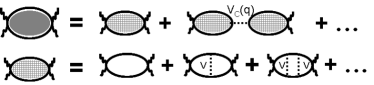
Figure 1: The summation scheme to calculate the non-resonant Raman response. The top line is the RPA sum involving the long-range Coulomb interaction $V_{C}({\vec{q}})$. The bottom line denotes the ladder approximation to account for the vertex corrections to the bare bubble. Here $V$ denotes a generic short-range interaction.

Figure 2: Diagrams in the ladder series for the Raman response that we call in the text particle-hole and particle-particle type contributions.

We obtain the generic expression for the Raman intensity, valid for any number of bands, any scattering geometry, and any spin-singlet gap symmetry. For demonstration purposes, later in the paper we focus on one-band and two-band 2D $s-$wave superconductors on a square lattice, in A_1g scattering geometry.

The general result, when applied to the one-band model, reproduces the result of Ref. [Lara, ] that the Raman intensity $R(\Omega)$ vanishes for a constant Raman vertex ($\gamma({\vec{k}})=$ const) due to vertex corrections. As an extension to that work, we expand the pairing interaction and the Raman vertex in $A_{1g}$ harmonics. We show that $R(\Omega)$ is finite when $\gamma({\vec{k}})$ has momentum dependence (e.g., $\cos{4\theta}$ harmonic in a 2D system on a square lattice). We show that the $2\Delta$ edge singularity in this $R(\Omega)$ is eliminated by vertex corrections, as long as the pairing interaction is also momentum-dependent, and is replaced by a maximum at a frequency above $2\Delta$. We argue that $R(\Omega)$ may also have $\delta$-function peaks at $\Omega<2\Delta$ due to BS-type and excitonic collective modes.

When applied to the two-band model, we reproduce another result of Ref. [Lara, ] that $R(\Omega)$ is non-zero when the Raman vertices $\gamma^{a}({\vec{k}})$, $a=1,2$, are different constants for the two bands. In addition to that work we also consider the case when $\gamma^{a}({\vec{k}})$ are momentum-dependent. We show that the $2\Delta$ peak in $R(\Omega)$ is again eliminated by vertex corrections and replaced by a maximum at a higher frequency. We analyze potential $\delta$-function peaks at $\Omega<2\Delta$ due to collective modes: Leggett collective mode in the particle-particle channel and excitonic collective mode in the particle-hole channel. In this analysis, we reproduce and generalize the results of Refs. [Lara, ] and [chubilya, ], respectively. We additionally consider the effects due to BS-type collective modes. We analyze in detail the interplay between the effects from collective modes in the particle-particle and particle-hole channels.

We next analyze the effect of the long-range Coulomb interaction. In graphical representation, this interaction creates series of additional renormalizations of the Raman bubble. All terms in these series contain the square of a fully renormalized bubble with the Raman vertex on one side and a total density vertex on the other. We demonstrate that such a bubble vanishes and hence the Coulomb interaction does not contribute to Raman scattering, even in $A_{1g}$ scattering geometry. We demonstrate this explicitly for the one-band model for a general $\gamma({\vec{k}})$, and for the two-band model for the case when $\gamma^{a}({\vec{k}})$ is momentum independent, but has different values for the two bands.

We also discuss some specific examples of the Raman scattering in 2D square-lattice systems in non-A_1g scattering geometry. In particular, we argue that for a $d-$wave superconductor, the Raman vertex in A_1g scattering geometry with $\gamma({\vec{k}})=$ const vanishes due to vertex renormalizations which involve the $d-$wave component of the interaction in the particle-particle channel, i.e., the one that gives rise to the pairing; while in a B_1g scattering geometry (with, e.g., $\gamma({\vec{k}})\propto\cos{2\theta}$), the renormalization of the bare Raman bubble in the particle-particle channel involves the $s$-wave component of the interaction in the particle-particle channel.

The rest of the text is organized as follows. In Sec II, we introduce an effective low energy model. In Sec III, we describe the generic computational scheme to calculate diagrammatically the Raman response with vertex corrections and screening. In Sec. IV, we apply this scheme to analyze vertex corrections within the Raman bubble. We consider one-band and two-band $s$-wave superconductors and $A_{1g}$ Raman scattering geometry and analyze the condition under which $R(\Omega)$ vanishes, the elimination of “$2\Delta$” edge singularity, and the effects due to Raman-active collective modes. In Sec. V, we discuss the role of Coulomb interaction and argue that it does not affect Raman scattering. In Sec. VI, we briefly discuss Raman intensity in other scattering geometries and for other gap symmetries, and consider a specific example of a $d-$wave superconductor and $A_{1g}$ and $B_{1g}$ scattering geometries. We present our conclusions in Sec. VII.

Figure 3: All possible interactions between a pair of bands $a,b$ (solid and dashed respectively). $V^{ab}_{1}$ is the density-density interaction between band $a$ and band $b$; $V^{ab}_{2}$ is an exchange between the two bands; $V_{3}$ is a Fermion-pair hopping term that is made possible due to Umpklapp processes; $V^{ab}_{4,5}$ are the density-density interaction terms within each band. Every pair of bands has a $V_{1,2,3}$ interaction component.

II The low energy model

We consider an effective low energy model of a superconductor with $N_{b}$ bands. The Hamiltonian is given by $\mathcal{H}=\mathcal{H}_{0}+\mathcal{H}_{\rm int}$, where $\mathcal{H}_{0}$ is the quadratic part, which includes the superconducting condensate, and $\mathcal{H}_{\rm int}$ is the combination of 4-fermion interaction terms. We assume that the pairing is in a spin-singlet channel, and that the condensates are made out of pairs of fermions with momenta ${{\vec{k}}}$ and $-{{\vec{k}}}$ from the same band. The quadratic Hamiltonian $\mathcal{H}_{0}$ is then diagonal in band basis: $\mathcal{H}_{0}=\sum_{a=1}^{N_{b}}\mathcal{H}_{a}$. Throughout the paper we use indices $a$ and $b$ to label the bands. We use the Nambu formalism and combine the fermionic creation and annihilation operators into a Nambu spinor $\Psi^{{\dagger}}_{a}({\vec{k}})\equiv(c^{{\dagger}}_{a,{\vec{k}},\uparrow},c_{a,-{\vec{k}},\downarrow},c^{{\dagger}}_{a,{\vec{k}},\downarrow},c_{a,-{\vec{k}},\uparrow})$. In this representation, $\mathcal{H}_{a}=\sum_{{\vec{k}}}\Psi^{{\dagger}}_{a}({\vec{k}})\mathcal{E}_{a}({\vec{k}})\Psi_{a}({\vec{k}})$, where the $4\times 4$ matrix $\mathcal{E}_{a}({\vec{k}})$ is given by

$$\mathcal{E}_{a}({\vec{k}})=\left(\begin{array}[]{cccc}\varepsilon^{a}_{\uparrow}({\vec{k}})&-\Delta^{a}_{\downarrow\uparrow}({\vec{k}})&0&0\\ -\Delta^{a*}_{\downarrow\uparrow}({\vec{k}})&-\varepsilon^{a}_{\downarrow}(-{\vec{k}})&0&0\\ 0&0&\varepsilon^{a}_{\downarrow}({\vec{k}})&-\Delta^{a}_{\uparrow\downarrow}({\vec{k}})\\ 0&0&-\Delta^{a*}_{\downarrow\uparrow}({\vec{k}})&-\varepsilon^{a}_{\uparrow}(-{\vec{k}})\end{array}\right)$$ (1)

The matrix $\mathcal{E}_{a}({\vec{k}})$ can be written in more compact form as $\mathcal{E}_{a}({\vec{k}})=\varepsilon^{a}Q^{a}_{3}-\Delta^{a}_{R}Q^{a}_{1}+\Delta^{a}_{I}Q^{a}_{2}$, where $Q^{a}_{i}=\sigma_{0}\otimes\sigma_{i}$ ($\sigma_{0}$ is $2\times 2$ identity matrix and $\sigma_{i}$ are the Pauli matrices), and $\Delta_{R,I}^{a}$ are the real and imaginary parts of the pairing gap $\Delta^{a}_{\downarrow\uparrow}({\vec{k}})$. The spinor space is spin$\otimes$Nambu (we use the same definition of the direct product as in Ref. direct, ). The $4\times 4$ Green’s function is then $G^{a}(\omega,{\vec{k}})=\left[i\omega\sigma_{0}-\mathcal{E}_{a}({{\vec{k}}})\right]^{-1}$. For spin-singlet pairing, the $4\times 4$ Nambu structure for $\mathcal{E}_{a}({{\vec{k}}})$ reduces to two equivalent $2\times 2$ structures, which differ by a spin-flip. We focus on one $2\times 2$ structure [the upper left $2\times 2$ part in Eq. (1)] and drop the $\sigma_{0}$ spin component from the spinor space. Then $\mathcal{E}_{a}$ and $G$ become $2\times 2$ matrices. All formulas below will be presented in this reduced space.

We approximate the interactions between low-energy band fermions in a superconductor as functions of the momentum transfer $q$. In doing so, we neglect the orbital composition of low-energy states, i.e., the fact that in many cases (e.g., Fe-pnictides/chalcogenides) band operators for low-energy states are linear combinations of fermions from different orbitals.rev2 Orbital physics generally induces additional momentum dependence of the interaction potentials via form-factors associated with the transformation from orbital to band basis for each fermion involved in the interaction. This complication, however, modifies the Raman response in a quantitative, but not in a qualitative way.hcs

We will need both unscreened and screened interactions for the computation of the Raman intensity. For the RPA renormalization of the Raman bubble we need the interaction at the Raman momentum transfer $q$. To avoid double counting we must treat this interaction $V_{C}(q)$ as unscreened [e.g., $V_{C}(q)=2\pi e^{2}/q$ in 2D]. For the renormalizations inside the Raman bubble (ladder series of renormalizations) we need interactions with a momentum transfer either of order $k_{F}$ or comparable to the distance $Q$ between different bands in momentum space, and with energy transfer comparable to $\Delta$. Such interactions should be taken as the screened ones. We assume that $v_{F}Q>v_{F}k_{F}>\Delta$, in which case screening transforms a bare long-range static Coulomb interaction into a short-range, but still static interaction. Accordingly, we approximate interactions inside the Raman bubble by constants, different for $q\sim k_{F}$ (intra-band) and $q\sim Q$ (inter-band).

In general, there are 4 types of intra-band and inter-band short-range interactions between low-energy fermions: density-density interaction between fermions from the same band and density-density, exchange and pair-hopping interactions between fermions from different bands (see Fig. 3). We use the same notations as in earlier worksChubukovPhysica ; AVCIE ; RGSM and label these interactions as $V_{4},V_{1}$, $V_{2}$, and $V_{3}$, respectively. Interactions of each type have additional band indices as the ones involving fermions from different bands are not necessarily equal. The intra-band interaction $V_{4}$ is diagonal in band basis and we label its components as $V^{aa}_{4}$. Interactions $V_{1},V_{2}$, and $V_{3}$ involve fermions from different bands, and we label their components as $V^{ab}_{1},V^{ab}_{2}$, and $V^{ab}_{3}$. There are ${N_{B}}\choose{2}$ pairs of bands $(a,b)$ with $a\neq b$. In Nambu notations the four interactions are

$$\mathcal{H}_{\text{int}} = \frac{1}{2}\left(H_{4}+H_{1}+H_{2}+H_{3}\right),$$ (2)

$$H_{4} = \sum_{a}\sum_{{\vec{q}}}V^{aa}_{4}(q)\sum_{{\vec{k}}}\Psi^{{\dagger}}_{a}({\vec{k}})\sigma_{3}\Psi_{a}({\vec{k}}+{\vec{q}})\sum_{{\vec{k}}^{\prime}}\Psi^{{\dagger}}_{a}({\vec{k}}^{\prime}+{\vec{q}})\sigma_{3}\Psi_{a}({\vec{k}}^{\prime})$$ (3)

$$H_{1} = \sum_{a\neq b}\sum_{{\vec{q}}}V^{ab}_{1}(q)\sum_{{\vec{k}}}\Psi^{{\dagger}}_{a}({\vec{k}})\sigma_{3}\Psi_{a}({\vec{k}}+{\vec{q}})\sum_{{\vec{k}}^{\prime}}\Psi^{{\dagger}}_{b}({\vec{k}}^{\prime}+{\vec{q}})\sigma_{3}\Psi_{b}({\vec{k}}^{\prime})$$ (4)

$$H_{2} = \sum_{a\neq b}\sum_{{\vec{q}}}V^{ab}_{2}(q)\times$$ (5)

$$\sum_{{\vec{k}}}\left(\Psi^{{\dagger}}_{a}({\vec{k}})\sigma_{+}\Psi_{b}({\vec{k}}+{\vec{q}})+\Psi^{{\dagger}}_{b}({\vec{k}})\sigma_{-}\Psi_{a}({\vec{k}}+{\vec{q}})\right)\sum_{{\vec{k}}^{\prime}}\left(\Psi^{{\dagger}}_{b}({\vec{k}}^{\prime}+{\vec{q}})\sigma_{+}\Psi_{a}({\vec{k}}^{\prime})+\Psi^{{\dagger}}_{a}({\vec{k}}^{\prime}+{\vec{q}})\sigma_{-}\Psi_{b}({\vec{k}}^{\prime})\right)$$

$$H_{3} = \sum_{a\neq b}\sum_{{\vec{q}}}V^{ab}_{3}(q)\times$$ (6)

$$\sum_{{\vec{k}}}\left(\Psi^{{\dagger}}_{a}({\vec{k}})\sigma_{+}\Psi_{b}({\vec{k}}+{\vec{q}})+\Psi^{{\dagger}}_{b}({\vec{k}})\sigma_{-}\Psi_{a}({\vec{k}}+{\vec{q}})\right)\sum_{{\vec{k}}^{\prime}}\left(\Psi^{{\dagger}}_{a}({\vec{k}}^{\prime}+{\vec{q}})\sigma_{+}\Psi_{b}({\vec{k}}^{\prime})+\Psi^{{\dagger}}_{b}({\vec{k}}^{\prime}+{\vec{q}})\sigma_{-}\Psi_{a}({\vec{k}}^{\prime})\right)$$

where $\sigma_{\pm}=(\sigma_{3}\pm\sigma_{0})/2$. The long-range interaction with the bare Coulomb potential $V_{C}(q)$ is expressed as:

$$H_{C} = \frac{1}{4}\sum_{{\vec{q}}}V_{C}({\vec{q}})\sum_{a,b}\sum_{{\vec{k}}}\Psi^{{\dagger}}_{a}({\vec{k}})\sigma_{3}\Psi_{a}({\vec{k}}+{\vec{q}})\sum_{{\vec{k}}^{\prime}}\Psi^{{\dagger}}_{b}({\vec{k}}^{\prime}+{\vec{q}})\sigma_{3}\Psi_{b}({\vec{k}}^{\prime}).$$ (7)

We also need self-consistency conditions on the pairing gaps $\Delta^{a}_{\downarrow\uparrow}({\vec{k}})$. They represent the set of coupled non-linear equations, which involve interactions $V^{aa}_{4}$ and $V^{ab}_{3}$. In explicit form

$$\Delta^{a}_{\downarrow\uparrow}({\vec{k}}) = -\int_{K^{\prime}}V_{4}^{aa}({\vec{k}}-{\vec{k}}^{\prime})G^{a}_{12}(K^{\prime})$$ (8)

$$-\sum_{b\neq a}\int_{K^{\prime}}V_{3}^{ab}({\vec{k}}-{\vec{k}}^{\prime})G^{b}_{12}(K^{\prime}).$$

where $K^{\prime}=(\omega^{\prime},{\vec{k}}^{\prime})$, $\int_{K^{\prime}}\equiv T\sum_{\omega^{\prime}}\int d^{d}k^{\prime}/(2\pi)^{d}$, and $G^{a}_{12}$ is a non-diagonal component of the $2\times 2$ matrix Green’s function $G^{a}(\omega,{\vec{k}})=\left[i\omega\sigma_{0}-\mathcal{E}_{a}({{\vec{k}}})\right]^{-1}$. We now proceed to compute the Raman response.

III The Raman Response

To calculate the fully renormalized Raman intensity we use the computational scheme outlined in Fig. 1. The Raman intensity $R(\Omega)$ is proportional to the imaginary part of the Raman susceptibility $\chi_{R}(\Omega)$. The latter is given by the fully renormalized particle-hole bubble with Raman vertices on both sides. We use the short-range interaction from $\mathcal{H}_{\rm int}$ for the renormalizations within a given particle-hole bubble, and the long range Coulomb interaction for RPA renormalizations of the interaction-dressed bubbles (shaded ones in Fig. 1). We approximate vertex renormalizations within the bubble by the ladder series of vertex corrections. We argue that this procedure preserves gauge invariance, provided that the equation for the SC gap is also obtained within the ladder approximation. This scheme is a multiband generalization of the computational approach used in Refs. Klein, ; zawadowskii, .

In the Nambu formalism, the Raman vertex for band $a$ is $\gamma^{a}_{{\vec{k}}}\sigma_{3}$ and the density vertex, which we will need in RPA series, is $\sigma_{3}$. The bare Raman susceptibility is graphically represented by the particle-hole bubble with $\gamma^{a}_{{\vec{k}}}\sigma_{3}$ in the vertices:

$$\chi_{R,0}(Q)=-\sum_{a}\int_{K}\text{Tr}\left[\gamma^{a}\sigma_{3}{G}^{a}_{K}\gamma^{a}\sigma_{3}{G}^{a}_{K+Q}\right]$$ (9)

where $K=(\omega,{\vec{k}}),Q=(\Omega,{\vec{q}})$, and, we remind the reader, $\int_{K}\equiv T\sum_{n}\int d^{d}k/(2\pi)^{d}$. The ladder renormalizations within a given particle-hole bubble can be absorbed into the renormalization of one of Raman vertices: $\gamma^{a}({\vec{k}})\sigma_{3}\rightarrow\Gamma^{a}({\vec{k}})$. The same also holds for the renormalization of the density vertex: $\sigma_{3}\rightarrow{\bar{\Gamma}}^{a}({\vec{k}})$. Replacing one of $\gamma^{a}({\vec{k}})$ by $\Gamma^{a}({\vec{k}})$ in Eq. 9 and adding the series of RPA renormalizations by $V_{C}$, as shown in Fig. 1, we obtain the full Raman susceptibility in the form

$$\chi_{R}(Q) = [-\pi_{RR}(Q)]+[-\pi_{RC}(Q)][-V_{C}({\vec{q}})][-\pi_{CR}(Q)]+[-\pi_{RC}(Q)][-V_{C}({\vec{q}})][-\pi_{CC}(Q)][-V_{C}({\vec{q}})][-\pi_{CR}(Q)]+...$$ (10)

$$= -\pi_{RR}(Q)-\pi_{RC}(Q)\frac{V_{C}({\vec{q}})}{1-V_{C}({\vec{q}})\pi_{CC}(Q)}\pi_{CR}(Q),$$

where

$$\pi_{RR}(Q) = \sum_{a}\int_{K}\text{Tr}\left[\gamma^{a}({\vec{k}})\sigma_{3}{G}^{a}_{K}{\Gamma}^{a}({\vec{k}}){G}^{a}_{K+Q}\right],$$ (11)

$$\pi_{RC}(Q) = \sum_{a}\int_{K}\text{Tr}\left[\gamma^{a}({\vec{k}})\sigma_{3}{G}^{a}_{K}{\bar{\Gamma}}^{a}({\vec{k}}){G}^{a}_{K+Q}\right],$$ (12)

$$\pi_{CC}(Q) = \sum_{a}\int_{K}\text{Tr}\left[{\sigma_{3}}{G}^{a}_{K}{\bar{\Gamma}}^{a}({\vec{k}}){G}^{a}_{K+Q}\right].$$ (13)

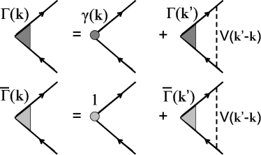
Figure 4: Schematic form of the integral vertex equations for $\Gamma({\vec{k}})$ and $\bar{\Gamma}({\vec{k}})$ (band indices have been dropped). The ‘1’ in the equation for $\bar{\Gamma}$ denotes the total density vertex (both $\gamma({\vec{k}})$ and ‘1’ are proportional to $\sigma_{3}$). Here $V({\vec{k}}^{\prime}-{\vec{k}})$ represents all the relevant short range interactions that enter the renormalization of the respective vertices. The solid lines with arrows denote Green’s function in Nambu space. The Green’s functions in the Nambu space are matrices constructed of normal and anomalous Green’s functions.

To evaluate $\pi_{RR}(Q),\pi_{RC}(Q)$, and $\pi_{CC}(Q)$, we need the expressions for the renormalized vertices $\Gamma^{a}({\vec{k}})$ and ${\bar{\Gamma}}^{a}({\vec{k}})$. The conventional way to obtain these expressions is to reduce the series of ladder diagrams for $\Gamma^{a}$ and ${\bar{\Gamma}}_{a}$ to integral equations in momentum, as schematically shown in Fig. 4, and solve these equations by expanding $\gamma^{a}(k)$, $\Gamma^{a}(k)$, and ${\bar{\Gamma}}_{a}(k)$ first in different irreducible representations and then in eigenfunctions for a given irreducible representation. We shall refer to the various components of this expansions as ‘partial components’. The partial components from different irreducible representations decouple, and the ones from the same irreducible representation form a set of linear algebraic equations. One set relates the prefactors for partial components of $\Gamma^{a}(k)$ to partial components of $\gamma^{a}(k)$, the other relates the prefactors for partial components of ${\bar{\Gamma}}_{a}(k)$ to the single non-zero partial component of the bare density vertex, which does not depend on $k$. This procedure, however, can be implemented in Nambu formalism only if the interaction can be factorized as $(\Psi^{{\dagger}}_{a}({\vec{k}})Q^{ab}\Psi_{b}({\vec{k}}+{\vec{q}}))\times(\Psi^{{\dagger}}_{b}({\vec{k}}^{\prime}+{\vec{q}})Q^{ba}\Psi_{a}({\vec{k}}^{\prime})$ with some matrices $Q^{ab}$ and $Q^{ba}$. The interactions $H_{4}$ and $H_{1}$ do have these forms (with $Q^{ab}=Q^{ba}=\sigma_{3}$), but $H_{2}$ and $H_{3}$ do not, as evident from (5) and (6). However, for the renormalization of the Raman bubble, we only need parts of $H_{2}$ and $H_{3}$ which do have the required forms. To see this we first observe that the Nambu matrix structure of the full $\Gamma^{a}({\vec{k}})$ and ${\bar{\Gamma}}_{a}({\vec{k}})$ is

$$\Gamma^{a}=\Gamma^{a}_{3}\sigma_{3}+\Gamma^{a}_{2}\sigma_{2},~{}~{}{\bar{\Gamma}}^{a}={\bar{\Gamma}}^{a}_{3}\sigma_{3}+{\bar{\Gamma}}^{a}_{2}\sigma_{2}.$$ (14)

This structure can be verified by directly evaluating the renormalized vertices in order-by-order calculations. The $\sigma_{3}$ structure is present in the bare vertices, and the renormalizations, which preserve it in the full $\Gamma^{a}({\vec{k}})$ and ${\bar{\Gamma}}_{a}({\vec{k}})$, involve, in the conventional Gorkov notation, the products of two normal and two anomalous Greens functions in each cross-section. We will be calling these as renormalizations in the “particle-hole” channel, because in the normal state they involve particle-hole pairs of intermediate fermions. The $\sigma_{2}$ structure comes from the processes which, in Gorkov notation, involve one normal and one anomalous Green’s function. Such processes transform a particle-hole vertex into a particle-particle one. We will be referring to these as renormalizations in the “particle-particle” channel. We next observe that the renormalizations in the particle-hole channel involve interactions $V^{aa}_{4}$ and $V^{ab}_{2}$ with the same spin projections for all four fermions, while the ones in the particle-particle channel involve $V^{aa}_{4}$ and $V^{ab}_{2}$ with opposite spin projection for two pairs fermions. The corresponding terms in $H_{2}$ and $H_{3}$ are

$$H_{2} \rightarrow \sum_{a\neq b}\sum_{{\vec{q}}}V^{ab}_{2}(q)\times$$ (15)

$$\sum_{{\vec{k}},{\vec{k}}^{\prime}}\left[\left(\Psi^{{\dagger}}_{a}({\vec{k}})\sigma_{+}\Psi_{b}({\vec{k}}+{\vec{q}})\right)\left(\Psi^{{\dagger}}_{b}({\vec{k}}^{\prime}+{\vec{q}})\sigma_{+}\Psi_{a}({\vec{k}}^{\prime})\right)\right]+\left(\Psi^{{\dagger}}_{a}({\vec{k}})\sigma_{-}\Psi_{b}({\vec{k}}+{\vec{q}})\right)\left(\Psi^{{\dagger}}_{b}({\vec{k}}^{\prime}+{\vec{q}})\sigma_{-}\Psi_{a}({\vec{k}}^{\prime})\right)$$

$$H_{3} \rightarrow \sum_{a\neq b}\sum_{{\vec{q}}}V^{ab}_{3}(q)\times$$ (16)

$$\sum_{{\vec{k}},{\vec{k}}^{\prime}}\left[\left(\Psi^{{\dagger}}_{a}({\vec{k}})\sigma_{+}\Psi_{b}({\vec{k}}+{\vec{q}})\right)\left(\Psi^{{\dagger}}_{b}({\vec{k}}^{\prime}+{\vec{q}})\sigma_{-}\Psi_{a}({\vec{k}}^{\prime})\right)+\left(\Psi^{{\dagger}}_{a}({\vec{k}})\sigma_{-}\Psi_{b}({\vec{k}}+{\vec{q}})\right)\left(\Psi^{{\dagger}}_{b}({\vec{k}}^{\prime}+{\vec{q}})\sigma_{+}\Psi_{a}({\vec{k}}^{\prime})\right)\right]$$

Both of these terms have $(\Psi^{{\dagger}}_{a}({\vec{k}})Q^{ab}\Psi_{b}({\vec{k}}+{\vec{q}}))\times(\Psi^{{\dagger}}_{b}({\vec{k}}^{\prime}+{\vec{q}})Q^{ba}\Psi_{b}({\vec{k}}^{\prime})$ Nambu matrix structure. Using these forms, and the one for the $V^{aa}_{4}$ interaction term, we obtain, after a simple algebra, the closed set of equations

$${\Gamma}^{a}_{3}({\vec{k}}) = \gamma^{a}({\vec{k}})-\frac{1}{2}\int_{K}V^{aa}_{4}({\vec{k}}-{\vec{k}}^{\prime})\text{Tr}\left[\sigma_{3}\left(\sigma_{3}{G}^{a}_{K^{\prime}}\right)\sigma_{3}\left({G}^{a}_{K^{\prime}+Q}\sigma_{3}\right)\right]{\Gamma}^{a}_{3}({\vec{k}}^{\prime})$$

$$-\frac{1}{2}\sum_{b\neq a}\int_{K}V^{ab}_{2}({\vec{k}}-{\vec{k}}^{\prime})\text{Tr}\left[\sigma_{3}\left(\sigma_{+}{G}^{b}_{K^{\prime}}\right)\sigma_{3}\left({G}^{b}_{K^{\prime}+Q}\sigma_{+}\right)+\sigma_{3}\left(\sigma_{-}{G}^{b}_{K^{\prime}}\right)\sigma_{3}\left({G}^{b}_{K^{\prime}+Q}\sigma_{-}\right)\right]{\Gamma}^{b}_{3}({\vec{k}}^{\prime})$$

$$-\frac{1}{2}\int_{K}V^{aa}_{4}({\vec{k}}-{\vec{k}}^{\prime})\text{Tr}\left[\sigma_{3}\left(\sigma_{3}{G}^{a}_{K^{\prime}}\right)\sigma_{2}\left({G}^{a}_{K^{\prime}+Q}\sigma_{3}\right)\right]{\Gamma}^{a}_{2}({\vec{k}}^{\prime})$$

$$-\frac{1}{2}\sum_{b\neq a}\int_{K}V^{ab}_{2}({\vec{k}}-{\vec{k}}^{\prime})\text{Tr}\left[\sigma_{3}\left(\sigma_{+}{G}^{b}_{K^{\prime}}\right)\sigma_{2}\left({G}^{b}_{K^{\prime}+Q}\sigma_{+}\right)+\sigma_{3}\left(\sigma_{-}{G}^{b}_{K^{\prime}}\right)\sigma_{2}\left({G}^{b}_{K^{\prime}+Q}\sigma_{-}\right)\right]{\Gamma}^{b}_{2}({\vec{k}}^{\prime})$$

$${\Gamma}^{a}_{2}({\vec{k}}) = -\frac{1}{2}\int_{K}V^{aa}_{4}({\vec{k}}-{\vec{k}}^{\prime})\text{Tr}\left[\sigma_{2}\left(\sigma_{3}{G}^{a}_{K^{\prime}}\right)\sigma_{2}\left({G}^{a}_{K^{\prime}+Q}\sigma_{3}\right)\right]{\Gamma}^{a}_{2}({\vec{k}}^{\prime})$$ (17)

$$-\frac{1}{2}\sum_{b\neq a}\int_{K}V^{ab}_{3}({\vec{k}}-{\vec{k}}^{\prime})\text{Tr}\left[\sigma_{2}\left(\sigma_{+}{G}^{b}_{K^{\prime}}\right)\sigma_{2}\left({G}^{b}_{K^{\prime}+Q}\sigma_{-}\right)+\sigma_{2}\left(\sigma_{-}{G}^{b}_{K^{\prime}}\right)\sigma_{2}\left({G}^{b}_{K^{\prime}+Q}\sigma_{+}\right)\right]{\Gamma}^{b}_{2}({\vec{k}}^{\prime})$$

$$-\frac{1}{2}\int_{K}V^{aa}_{4}({\vec{k}}-{\vec{k}}^{\prime})\text{Tr}\left[\sigma_{2}\left(\sigma_{3}{G}^{a}_{K^{\prime}}\right)\sigma_{3}\left({G}^{a}_{K^{\prime}+Q}\sigma_{3}\right)\right]{\Gamma}^{a}_{3}({\vec{k}}^{\prime})$$

$$-\frac{1}{2}\sum_{b\neq a}\int_{K}V^{ab}_{3}({\vec{k}}-{\vec{k}}^{\prime})\text{Tr}\left[\sigma_{2}\left(\sigma_{+}{G}^{b}_{K^{\prime}}\right)\sigma_{3}\left({G}^{b}_{K^{\prime}+Q}\sigma_{-}\right)+\sigma_{2}\left(\sigma_{-}{G}^{b}_{K^{\prime}}\right)\sigma_{3}\left({G}^{b}_{K^{\prime}+Q}\sigma_{+}\right)\right]{\Gamma}^{b}_{3}({\vec{k}}^{\prime}),$$

and

$${\bar{\Gamma}}^{a}_{3}({\vec{k}}) = 1-\frac{1}{2}\int_{K}V^{aa}_{4}({\vec{k}}-{\vec{k}}^{\prime})\text{Tr}\left[\sigma_{3}\left(\sigma_{3}{G}^{a}_{K^{\prime}}\right)\sigma_{3}\left({G}^{a}_{K^{\prime}+Q}\sigma_{3}\right)\right]{\bar{\Gamma}}^{a}_{3}({\vec{k}}^{\prime})$$

$$-\frac{1}{2}\sum_{b\neq a}\int_{K}V^{ab}_{2}({\vec{k}}-{\vec{k}}^{\prime})\text{Tr}\left[\sigma_{3}\left(\sigma_{+}{G}^{b}_{K^{\prime}}\right)\sigma_{3}\left({G}^{b}_{K^{\prime}+Q}\sigma_{+}\right)+\sigma_{3}\left(\sigma_{-}{G}^{b}_{K^{\prime}}\right)\sigma_{3}\left({G}^{b}_{K^{\prime}+Q}\sigma_{-}\right)\right]{\bar{\Gamma}}^{b}_{3}({\vec{k}}^{\prime})$$

$$-\frac{1}{2}\int_{K}V^{aa}_{4}({\vec{k}}-{\vec{k}}^{\prime})\text{Tr}\left[\sigma_{3}\left(\sigma_{3}{G}^{a}_{K^{\prime}}\right)\sigma_{2}\left({G}^{a}_{K^{\prime}+Q}\sigma_{3}\right)\right]{\bar{\Gamma}}^{a}_{2}({\vec{k}}^{\prime})$$

$$-\frac{1}{2}\sum_{b\neq a}\int_{K}V^{ab}_{2}({\vec{k}}-{\vec{k}}^{\prime})\text{Tr}\left[\sigma_{3}\left(\sigma_{+}{G}^{b}_{K^{\prime}}\right)\sigma_{2}\left({G}^{b}_{K^{\prime}+Q}\sigma_{+}\right)+\sigma_{3}\left(\sigma_{-}{G}^{b}_{K^{\prime}}\right)\sigma_{2}\left({G}^{b}_{K^{\prime}+Q}\sigma_{-}\right)\right]{\bar{\Gamma}}^{b}_{2}({\vec{k}}^{\prime})$$

$${\bar{\Gamma}}^{a}_{2}({\vec{k}}) = -\frac{1}{2}\int_{K}V^{aa}_{4}({\vec{k}}-{\vec{k}}^{\prime})\text{Tr}\left[\sigma_{2}\left(\sigma_{3}{G}^{a}_{K^{\prime}}\right)\sigma_{2}\left({G}^{a}_{K^{\prime}+Q}\sigma_{3}\right)\right]{\bar{\Gamma}}^{a}_{2}({\vec{k}}^{\prime})$$ (18)

$$-\frac{1}{2}\sum_{b\neq a}\int_{K}V^{ab}_{3}({\vec{k}}-{\vec{k}}^{\prime})\text{Tr}\left[\sigma_{2}\left(\sigma_{+}{G}^{b}_{K^{\prime}}\right)\sigma_{2}\left({G}^{b}_{K^{\prime}+Q}\sigma_{-}\right)+\sigma_{2}\left(\sigma_{-}{G}^{b}_{K^{\prime}}\right)\sigma_{2}\left({G}^{b}_{K^{\prime}+Q}\sigma_{+}\right)\right]{\bar{\Gamma}}^{b}_{2}({\vec{k}}^{\prime})$$

$$-\frac{1}{2}\int_{K}V^{aa}_{4}({\vec{k}}-{\vec{k}}^{\prime})\text{Tr}\left[\sigma_{2}\left(\sigma_{3}{G}^{a}_{K^{\prime}}\right)\sigma_{3}\left({G}^{a}_{K^{\prime}+Q}\sigma_{3}\right)\right]{\bar{\Gamma}}^{a}_{3}({\vec{k}}^{\prime})$$

$$-\frac{1}{2}\sum_{b\neq a}\int_{K}V^{ab}_{3}({\vec{k}}-{\vec{k}}^{\prime})\text{Tr}\left[\sigma_{2}\left(\sigma_{+}{G}^{b}_{K^{\prime}}\right)\sigma_{3}\left({G}^{b}_{K^{\prime}+Q}\sigma_{-}\right)+\sigma_{2}\left(\sigma_{-}{G}^{b}_{K^{\prime}}\right)\sigma_{3}\left({G}^{b}_{K^{\prime}+Q}\sigma_{+}\right)\right]{\bar{\Gamma}}^{b}_{3}({\vec{k}}^{\prime}).$$

Evaluating the traces over Pauli matrices, we then obtain the set of coupled integral equations in momentum for $\Gamma^{a}_{2,3}({\vec{k}})$ and ${\bar{\Gamma}}^{a}_{2,3}({\vec{k}})$. Each $\Gamma^{a}_{2,3}({\vec{k}})$ is expressed via $\int d^{d}k^{\prime}$ over $\Gamma^{b}_{2,3}({\vec{k}}^{\prime})$ with a kernel, that depends on ${\vec{k}}^{\prime}$ and ${\vec{k}}-{\vec{k}}^{\prime}$. The same holds for ${\bar{\Gamma}}^{a}_{2,3}$. We then separate different irreducible lattice representations, (e.g., one-dimensional representations $A_{1g},B_{1g},B_{2g},A_{2g}$ for the 2D square lattice), and expand momentum-dependent interactions $V^{aa}_{4}({\vec{k}}-{\vec{k}}^{\prime}),V_{2}^{ab}({\vec{k}}-{\vec{k}}^{\prime})$, $V_{3}^{ab}({\vec{k}}-{\vec{k}}^{\prime})$, and the vertices $\Gamma^{a}_{2}({\vec{k}})$, $\Gamma^{a}_{3}({\vec{k}})$, ${\bar{\Gamma}}^{a}_{2}({\vec{k}})$, ${\bar{\Gamma}}^{a}_{3}({\vec{k}})$, into the set of orthogonal eigenfunctions within a given representation as

$$V_{4}^{aa}({\vec{k}}-{\vec{k}}^{\prime})=\sum_{..}\sum_{tp}f^{t}_{{\vec{k}}}V_{4}^{aa,tp}f^{p}_{{\vec{k}}^{\prime}},$$

$$V_{2,3}^{ab}({\vec{k}}-{\vec{k}}^{\prime})=\sum_{..}\sum_{tp}f^{t}_{{\vec{k}}}V_{2,3}^{ab,tp}f^{p}_{{\vec{k}}^{\prime}},$$

$$\Gamma^{a}_{2}({\vec{k}})\sum_{..}\sum_{t}\Gamma^{a,t}_{2}f^{t}_{{\vec{k}}},~{}\Gamma^{a}_{3}({\vec{k}})=\sum_{..}\sum_{t}\Gamma^{a,t}_{3}f^{t}_{{\vec{k}}},$$

$${\bar{\Gamma}}^{a}_{2}({\vec{k}})=\sum_{..}\sum_{t}{\bar{\Gamma}}^{a,t}_{2}f^{t}_{{\vec{k}}},~{}{\bar{\Gamma}}^{a}_{3}({\vec{k}})=\sum_{..}\sum_{t}{\bar{\Gamma}}^{a,t}_{3}f^{t}_{{\vec{k}}}.$$ (19)

where $\sum_{..}$ stands for the sum over representations. We also expand the Raman vertex

$$\gamma^{a}({\vec{k}})=\sum_{..}\sum_{t}c^{a}_{t}f^{t}_{{\vec{k}}}.$$ (20)

Substituting this into Eqs. (17) and (18), separating the components, and using the fact that eigenfunctions from different representations are orthogonal, we obtain the set of equations for the partial components within a given representation

$${\Gamma}^{a,t}_{3} = c^{a}_{t}-\frac{1}{2}\int_{K}\left[\sum_{p,m}\left(V^{aa,tp}_{4}\left(\Pi^{aa,pm}_{32}\Gamma_{2}^{a,m}+\Pi^{aa,pm}_{33}\Gamma_{3}^{a,m}\right)+\sum_{b}V^{ab,tp}_{2}\left(\Pi^{bb,pm}_{32}\Gamma_{2}^{b,m}+\Pi^{bb,pm}_{33}\Gamma_{3}^{b,m}\right)\right)\right]$$

$${\Gamma}^{a,t}_{2} = \frac{1}{2}\int_{K}\left[\sum_{p,m}\left(V^{aa,tp}_{4}\left(\Pi^{aa,pm}_{22}\Gamma_{2}^{a,m}+\Pi^{aa,pm}_{23}\Gamma_{3}^{a,m}\right)+\sum_{b}V^{ab,tp}_{3}\left(\Pi^{bb,pm}_{22}\Gamma_{2}^{b,m}+\Pi^{bb,pm}_{23}\Gamma_{3}^{b,m}\right)\right)\right]$$

$${\bar{\Gamma}}^{a,t}_{3} = \delta_{t,1}-\frac{1}{2}\int_{K}\left[\sum_{p,m}\left(V^{aa,tp}_{4}\left(\Pi^{aa,pm}_{32}{\bar{\Gamma}}_{2}^{a,m}+\Pi^{aa,pm}_{33}{\bar{\Gamma}}_{3}^{a,m}\right)+\sum_{b}V^{ab,tp}_{2}\left(\Pi^{bb,pm}_{32}{\bar{\Gamma}}_{2}^{b,m}+\Pi^{bb,pm}_{33}{\bar{\Gamma}}_{3}^{b,m}\right)\right)\right]$$

$${\bar{\Gamma}}^{a,t}_{2} = \frac{1}{2}\int_{K}\left[\sum_{p,m}\left(V^{aa,tp}_{4}\left(\Pi^{aa,pm}_{22}{\bar{\Gamma}}_{2}^{a,m}+\Pi^{aa,pm}_{23}{\bar{\Gamma}}_{3}^{a,m}\right)+\sum_{b}V^{ab,tp}_{3}\left(\Pi^{bb,pm}_{22}{\bar{\Gamma}}_{2}^{b,m}+\Pi^{bb,pm}_{23}{\bar{\Gamma}}_{3}^{b,m}\right)\right)\right]$$ (21)

where

$$\Pi^{ab,pm}_{ij}=\int_{K^{\prime}}f^{p}_{{\vec{k}}^{\prime}}f^{m}_{{\vec{k}}^{\prime}}\text{Tr}\left[\sigma_{i}G^{a}_{K^{\prime}}\sigma_{j}G^{b}_{K^{\prime}+Q}\right].$$ (22)

We remind the reader that $a,b$ label bands, $p,m$ label partial components, and $i,j=2,3$ label the two sigma-matrices $\sigma_{2}$ and $\sigma_{3}$. Note that $\Pi^{ab,pm}_{ij}$ with different $p$ and $m$ is generally non-zero, because the corresponding eigenfunctions belong to the same irreducible representation (e.g., $f^{1}_{{\vec{k}}}=1,f^{2}_{{\vec{k}}}=\sqrt{2}\cos{4\theta}$, etc for $A_{1g}$ representation in 2D, at $|{\vec{k}}|=k_{F}$). Eqs. (21) can be cast into the matrix forms

$$\sum_{b,j,p}R^{ab,tp}_{ij}\Gamma_{j}^{b,p}=c^{a}_{t}\delta_{i,3} \rightarrow [\mathcal{R}][\Gamma]=[c]$$

$$\sum_{b,j,p}R^{ab,tp}_{ij}\bar{\Gamma}_{j}^{b,p}=\delta_{t,0}\delta_{i,3} \rightarrow [\mathcal{R}][\bar{\Gamma}]=[\bar{c}].$$ (23)

Here $[\mathcal{R}]$ is the square matrix with dimensions $2N_{b}n\times 2N_{b}n$ where $n$ is the number of components that we keep in Eq. (III). The matrices $[\Gamma],[\bar{\Gamma}],[c]$, and $[\bar{c}]$ are vectors with the dimension $2N_{b}n$.

The matrix $[\mathcal{R}]$ is determined by Eq. (21). It can be cast into the form:

$$\mathcal{R}_{2N_{B}n\times 2N_{B}n}=\left[1+\frac{1}{2}[V_{pp}][\Pi_{pp}]+\frac{1}{2}[V_{ph}][\Pi_{ph}]\right],$$ (24)

where

$$[V_{pp}]=\left(\begin{array}[]{ccccccc}V^{11,11}_{4}&V^{12,11}_{3}...&V^{1N_{b},11}_{3}&V^{11,12}_{4}&V^{12,12}_{3}...&V^{1N_{b},12}_{3}&...\\ V^{21,11}_{3}&V^{22,11}_{4}...&V^{2N_{b},11}_{3}&V^{21,12}_{3}&V^{22,12}_{4}...&V^{2N_{b},12}_{3}&...\\ &&&.&&&\\ &&&.&&&\\ &&&.&&&\\ V^{Nb1,n1}_{3}&V^{N_{b}2,n1}_{3}...&V^{N_{b}N_{b},n1}_{4}&V^{N_{b}1,n2}_{3}&V^{22,n2}_{3}...&V^{N_{b}N_{b},n2}_{4}&...\end{array}\right)_{N_{b}n\times N_{b}n}\otimes\mathbb{1}_{2\times 2}$$ (31)

and $[V_{ph}]$ has the same form as $[V_{pp}]$ with $V_{3}\rightarrow V_{2}$. The matrix $[\Pi_{pp}]$ is given by

$$[\Pi_{pp}]=\left(\begin{array}[]{ccccccc}P^{11,11}&0_{2\times 2}...&0_{2\times 2}&P^{11,12}&0_{2\times 2}...&0_{2\times 2}&...\\ 0_{2\times 2}&P^{22,11}...&0_{2\times 2}&0_{2\times 2}&P^{22,12}...&0_{2\times 2}&...\\ &&&.&&&\\ &&&.&&&\\ &&&.&&&\\ 0_{2\times 2}&0_{2\times 2}...&0_{2\times 2}&P^{N_{b}N_{b},n1}&0_{2\times 2}...&P^{N_{b}N_{b},n2}&...\end{array}\right)_{N_{b}n\times N_{b}n},~{}~{}~{}~{}~{}~{}~{}~{}~{}~{}~{}~{}~{}~{}~{}~{}~{}~{}~{}~{}~{}~{}$$ (32)

where

$$P^{aa,mt}=\left(\begin{array}[]{cc}-\Pi^{aa,mt}_{22}&-\Pi^{aa,mt}_{23}\\ 0&0\end{array}\right),~{}0_{2\times 2}=\left(\begin{array}[]{cc}0&0\\ 0&0\end{array}\right).$$ (33)

The matrix $[\Pi_{ph}]$ is the same as $[\Pi_{pp}]$, with $P\rightarrow\tilde{P}$, where

$$\tilde{P}^{aa,mt}=\left(\begin{array}[]{cc}0&0\\ \Pi^{aa,mt}_{32}&\Pi^{aa,mt}_{33}\end{array}\right).$$ (34)

Finally,

$$[c]^{T} = (C^{1}_{1},C^{2}_{1},..C^{N_{b}}_{1},C^{1}_{2},...C^{N_{b}}_{2},...);$$

$$C^{a}_{t} = (0,c^{a}_{t}),$$ (35)

and

$$[\bar{c}]^{T} = (\bar{C}^{1}_{1},\bar{C}^{2}_{1},..\bar{C}^{N_{b}}_{1},0,...0,...);$$

$$\bar{C}^{a}_{1} = (0,1).$$ (36)

Using the above expressions we obtain

$$\pi_{RR} = \sum_{a}\sum_{t_{1}t_{2}}\sum_{j=2,3}c_{t_{1}}^{a}\Pi^{aa,t_{1}t_{2}}_{3j}{\Gamma}^{a,t_{2}}_{j},$$ (37)

$$\pi_{RC} = \sum_{a}\sum_{t_{1}t_{2}}\sum_{j=2,3}c_{t_{1}}^{a}\Pi^{aa,t_{1}t_{2}}_{3j}{\bar{\Gamma}}^{a,t_{2}}_{j},$$ (38)

$$\pi_{CR} = \sum_{a}\sum_{t_{1}t_{2}}\sum_{j=2,3}\delta_{t_{1},1}\Pi^{aa,t_{1}t_{2}}_{3j}{\Gamma}^{a,t_{2}}_{j},$$ (39)

$$\pi_{CC} = \sum_{a}\sum_{t_{1}t_{2}}\sum_{j=2,3}\delta_{t_{1},1}\Pi^{aa,t_{1}t_{2}}_{3j}{\bar{\Gamma}}^{a,t_{2}}_{j}.$$ (40)

All these quantities depend on $Q=(\Omega,{\vec{q}})$ via the polarization operators. The quantities $\pi_{CR}$ and $\pi_{RC}$ are indeed equal. Eqs. (37) - (40) together with the Eq. (10) relating $\pi_{RR},\pi_{RC}=\pi_{CR}$ and $\pi_{CC}$ to Raman susceptibility $\chi_{R}(\Omega,{\vec{q}})$ comprise the general formula for the Raman intensity $R(\Omega)\propto\text{Im}\chi_{R}(\Omega,q\to 0)$. These relations are valid for any number of bands, any pairing symmetry, and any Raman scattering geometry. Raman-active collective modes show up as poles in $\chi_{R}(\Omega,{\vec{q}})$ and spikes in $R(\Omega)$.

In the next two sections (Sec. IV and Sec. V), we present a case-by-case analysis of the $A_{\rm 1g}$ Raman intensity at $T=0$ in one-band and two-band 2D $s-$wave SCs on a square lattice. In Sec. IV, we investigate the response without Coulomb interaction, i.e. approximate $\chi_{R}(\Omega)$ by $-\pi_{RR}(\Omega)$. We consider separately the effects due to renormalizations of the Raman bubble in the particle-particle and particle-hole channels. In Sec. V we discuss the contribution to Raman response from Coulomb interaction.

IV Application to A_1g channel

It is clear that from Eqs. 37-40 that essential quantities needed for the Raman response Fare the polarization bubbles $\Pi_{ij}^{aa,mt}$ for various harmonics belonging to the A_1g representation: $\{1,\cos k_{x}+\cos k_{y},...\}$ over the BZ, or $f_{{\vec{k}}}=\{1,\cos 4\theta,\cos 8\theta,...\}$ over the Fermi-surface, where $\theta$ is the angle which ${\vec{k}}$ makes with the $k_{x}$ axis in the BZ. In general, the pairing gap $\Delta$ and the density of states on the Fermi surface $\nu_{F}$ also contain infinite number of $A_{1g}$ components. For the sake of transparency, we assume that $\Delta$ and the density of states $\nu_{F}$ are isotropic. These assumptions are made only to simplify the presentation and be able to compute $\chi_{R}(\Omega)$ analytically.

IV.1 One-band $s$-wave SC

We start with the one-band case – one FS, centered at the $\Gamma$-point. This case has been analyzed diagrammatically by Klein and Dierker,Klein and we indeed reproduce their results. In contrast to Ref. Klein, , however, we analyze the effects of short-range and Coulomb interactions separately. We show that there is a strong reduction [and full cancellation for $\gamma({\vec{k}})=$const] of the $A_{1g}$ Raman response already due to vertex corrections in the particle-particle channel. This was not emphasized in Ref. [Klein, ], although it follows from the formulas presented in that work. The reduction/cancellation of $A_{\rm 1g}$ response due to vertex corrections has been demonstrated in Ref. [ Lara, ], where the authors used effective action approach rather than direct diagrammatics.

IV.1.1 Isotropic case

In an isotropic case, there is only one component of $f_{{\vec{k}}}$ and $\gamma_{{\vec{k}}}$ in A_1g geometry: $f_{{\vec{k}}}=1,\gamma_{{\vec{k}}}=c_{1}$. For the one-band model, the only interaction is $V^{11,11}_{4}=V_{4}$, and we take it to be attractive, i.e., $V_{4}<0$. To compute the Raman response, we need the expressions for four $2\times 2$ matrices $\Pi_{ij}^{11,11}=\Pi_{ij}$ with $i,j=2,3$. Evaluating $\Pi_{ij}=\int_{K^{\prime}}Tr\left[\sigma_{i}G^{1}_{K^{\prime}}\sigma_{j}G^{1}_{K^{\prime}+Q}\right]$, we obtain

$$[V_{pp}]=V_{4}\sigma_{0};~{}[\Pi_{pp}]=\left(\begin{array}[]{cc}-\Pi_{22}&-\Pi_{23}\\ 0&0\end{array}\right)$$

$$[V_{ph}]=V_{4}\sigma_{0};~{}[\Pi_{ph}]=\left(\begin{array}[]{cc}0&0\\ \Pi_{32}&\Pi_{33}\\ \end{array}\right),$$ (41)

where, as before, $\sigma_{0}$ is the $2\times 2$ unity matrix, and

$$\Pi_{22}(\Omega) = \frac{2}{V_{4}}-\left(\frac{\Omega}{2\Delta}\right)^{2}F(\Omega),$$

$$\Pi_{23}(\Omega) = \frac{i\Omega}{2\Delta}F(\Omega),$$

$$\Pi_{32}(\Omega) = -\Pi_{23}(\Omega),$$

$$\Pi_{33}(\Omega) = -F(\Omega),$$ (42)

where

$$F(\Omega) = \int_{{\vec{k}}}\frac{\Delta^{2}}{E_{{\vec{k}}}\left[E^{2}_{{\vec{k}}}-(\Omega/2)^{2}\right]}$$

$$= 2\nu_{F}\frac{\sin^{-1}\left(\Omega/2\Delta\right)}{(\Omega/2\Delta)\sqrt{1-\left(\Omega/2\Delta\right)^{2}}}$$

$$E_{{\vec{k}}} = \sqrt{[\epsilon({\vec{k}})]^{2}+\Delta^{2}},$$ (43)

In Eq. (IV.1.1) we used self-consistency condition on $\Delta$, Eq. (8) at $T=0$ which yields

$$\int_{{\vec{k}}}\frac{1}{2E_{{\vec{k}}}}=-\frac{1}{V_{4}}.$$ (44)

The matrix $[c]^{T}$ is $(0,c_{1})$, and

$$\mathcal{R}\equiv\left(\begin{array}[]{cc}\mathcal{R}_{22}&\mathcal{R}_{23}\\ \mathcal{R}_{32}&\mathcal{R}_{33}\end{array}\right)=\sigma_{0}+\frac{1}{2}[V_{pp}][\Pi_{pp}]+\frac{1}{2}[V_{ph}][\Pi_{ph}]$$ (45)

$$~{}~{}~{}~{}~{}=\left(\begin{array}[]{cc}1-\frac{V_{4}}{2}\Pi_{22}&-\frac{V_{4}}{2}\Pi_{23}\\ \frac{V_{4}}{2}\Pi_{32}&1+\frac{V_{4}}{2}\Pi_{33}\end{array}\right).$$ (46)

Calculating $[\Gamma]$ as $[\mathcal{R}]^{-1}[c]$ from Eq. (III) and using Eq. (37), we see that the Raman response $\chi_{R}(\Omega)$ is given by

$$\chi_{R}(\Omega) = (c_{1})^{2}\frac{\Pi_{32}\mathcal{R}_{23}-\Pi_{33}\mathcal{R}_{22}}{\text{Det}[\mathcal{R}]}$$ (47)

$$= -(c_{1})^{2}\left[\frac{\Pi_{33}-\frac{(\Pi_{23})^{2}}{2/V_{4}-\Pi_{22}}}{1+\frac{V_{4}}{2}\left(\Pi_{33}-\frac{(\Pi_{23})^{2}}{2/V_{4}-\Pi_{22}}\right)}\right]$$

IV.1.2 Role of $V_{pp}$

Let us first analyze only vertex corrections in the particle-particle channel. To do this, we momentarily set $[V_{ph}]$ term in Eq. 24 to zero. We denote the corresponding Raman response as $\chi_{R}^{pp}(\Omega)$. We obtain

$$\chi_{R}^{pp}(\Omega)=-(c_{1})^{2}\left\{\Pi_{33}-\frac{(\Pi_{23})^{2}}{\frac{2}{V_{4}}-\Pi_{22}}\right\}$$ (48)

Substituting the expressions for $\Pi_{ij}$ from Eq. (IV.1.1), we find that $\chi_{R}^{pp}(\Omega)$ vanishes:

$$\chi_{R}^{pp}(\Omega) = (c_{1})^{2}\left\{F(\Omega)-\frac{(\Omega/2)^{2}F^{2}(\Omega)}{\frac{2}{V_{4}}-\frac{2}{V_{4}}+(\Omega/2)^{2}F(\Omega)}\right\}$$ (49)

$$= 0.$$

The first $F(\Omega)$ term in Eq. (49) is a free-fermion particle-hole polarization bubble. Taken alone, this term would give rise to $2\Delta$ singularity in the Raman response and to non-zero Raman intensity $\propto\text{Im}[\chi^{pp}_{R}(\Omega)]$ at $\Omega>2\Delta$. The second term, that cancels $F(\Omega)$, is the contribution from vertex corrections in the particle-particle channel. The cancellation of the two $\frac{2}{V_{4}}$ in the denominator of Eq. (49) is guaranteed by the U(1)-gauge invariance: the Raman susceptibility must contain the pole corresponding to the BAG mode, and the vanishing of the denominator in Eq. (49) at $\Omega=0$ ensures that this mode is massless. The vanishing of $\chi^{pp}_{R}(\Omega)$ at all frequencies is the consequence of the conservation of the number of fermions (or, equivalently, of the total charge). Indeed, for $\gamma_{{\vec{k}}}=c_{1}$, the Raman vertex becomes identical to the density vertex, and particle conservation imposes that the density-density bubble must vanish at ${\vec{q}}\rightarrow 0$ and any finite $\Omega$. We emphasize that this vanishing holds independent of whether we include long-range Coulomb interaction.

Despite the vanishing of $\chi^{pp}({\Omega})$ is expected in an isotropic case on general grounds, it has not been discussed in Raman literature until recently.Lara Several authorsdev_2 ; Deveaux ; Klein ; PeterBoyd ; Girsh presented results for A_1g Raman intensity that vanishes due to screening by long-range Coulomb interaction if $\gamma({\vec{k}})$ is treated as a constant. Our analysis (and the one in Ref. Lara, ) shows that the $A_{1g}$ Raman intensity in an $s-$wave SC vanishes in the isotropic case already before one includes long-range Coulomb interaction. The physics argument is that the original, normal state Hamiltonian with four-fermion interaction $V_{pp}$ conserves the number of particles, hence once all effects due to $V_{pp}$ are included (i.e., the contributions from the superconducting condensate and from renormalizations in the particle-particle channel within the particle-hole bubble), the fully dressed density-density bubble should obey the same conservations laws as in the normal state, i.e., it should vanish at $q=0$ and finite $\Omega$.

$\begin{array}[]{c}\includegraphics[width=195.12767pt]{oneband_a}\\ \includegraphics[width=195.12767pt]{oneband_b}\\ \end{array}$

Figure 5: Color online: (a) The Raman response, for a 1-band $s-$wave SC in the A_1g channel, where it is approximated by the bare bubble contribution (dashed green line), the vertex corrected (VC) contribution with a constant $\gamma_{{\vec{k}}}$ (red line) and VC contribution with a momentum dependent $\gamma_{{\vec{k}}}$ (black line). (b) The removal of the $2\Delta$ edge singularity by vertex corrections from the subleading channel interaction $v^{22}_{4}\equiv\nu_{F}V_{4}^{22}$. The peak shifts to larger $\Omega$ as the interaction strength in increased. We have used $V^{11}_{4}=-0.3/\nu_{F}$, $c_{1}=0.3,~{}c_{2}=0.2$. A fermion lifetime of $0.005\Delta$ was added to obtain the broadening.

IV.1.3 Role of $V_{ph}$

We now show that $A_{1g}$ Raman intensity in the isotropic case still vanishes, even if we include the renormalizations in the particle-hole channel. Indeed, comparing Eqs. (47) and (48) we immediately find that

$$\chi_{R}(\Omega) = \frac{\chi_{R}^{pp}(\Omega)}{1-\frac{V_{4}}{2c^{2}_{1}}\chi_{R}^{pp}(\Omega)}$$ (50)

Because $\chi_{R}^{pp}(\Omega)=0$, the full Raman response, with particle-particle and particle-hole vertex corrections, also vanishes. This is indeed expected because $V_{ph}$ preserves the number of particles.

IV.2 Case of anisotropic Raman vertex for one-band SC

We now consider the case when the Raman vertex has two partial components (from the same irreducible representation): $\gamma_{{\vec{k}}}=c_{1}f^{1}_{{\vec{k}}}+c_{2}f^{2}_{{\vec{k}}}$. For definiteness we take $f^{1}_{{\vec{k}}}=1,f^{2}_{{\vec{k}}}=\sqrt{2}\cos{4\theta}$. We use Eq. (III) to decompose $V_{4}({\vec{q}})=V_{4}({\vec{k}}-{\vec{k}}^{\prime})$ into two harmonics

$$V_{4}({\vec{k}}-{\vec{k}}^{\prime}) = f^{1}_{{\vec{k}}}V_{4}^{11}f^{1}_{{\vec{k}}^{\prime}}+f^{2}_{{\vec{k}}}V_{4}^{22}f^{2}_{{\vec{k}}^{\prime}}+$$ (51)

$$f^{1}_{{\vec{k}}}V_{4}^{12}f^{2}_{{\vec{k}}^{\prime}}+f^{2}_{{\vec{k}}}V_{4}^{21}f^{1}_{{\vec{k}}^{\prime}}$$

$$= V_{4}^{11}+2V_{4}^{22}{\cos{4\theta_{k}}}{\cos{4\theta_{k^{\prime}}}}+$$

$$\sqrt{2}V_{4}^{12}\left({\cos{4\theta_{k}}}+{\cos{4\theta_{k^{\prime}}}}\right).$$

The off-diagonal terms can be eliminated by a rotation to new eigenfunctions,SMPJH which are linear combinations of a constant and ${\cos{4\theta_{k}}}$. We will not do this, but just set here $V_{4}^{12}=V_{4}^{21}=0$. We will discuss a more generic case in Sec. V, when we analyze the role of Coulomb interaction. As before, we assume that SC is induced by the interaction $V_{4}^{11}$, which we keep negative (attractive). The corresponding gap $\Delta$ is then isotropic. The interaction $V_{4}^{22}$ can be either repulsive or attractive. In the latter case, we assume that it is weaker than $V_{4}^{11}$.

The matrices $[V_{pp}]$ and $[V_{ph}]$ now become $4\times 4$ matrices ($N_{b}=1,n=2$, $2N_{b}n=4$). We have (dropping the band indices $ab$, i.e., setting $V^{ab,mt}_{i}=V^{mt}_{i},\Pi_{ij}^{ab,mt}=\Pi_{ij}^{mt}$)

$$[V_{pp}]=\left(\begin{array}[]{cc}V_{4}^{11}\sigma_{0}&0\\ 0&V_{4}^{22}\sigma_{0}\end{array}\right);~{}[V_{ph}]=\left(\begin{array}[]{cc}V_{4}^{11}\sigma_{0}&0\\ 0&V_{4}^{22}\sigma_{0}\end{array}\right);$$

The matrices $[\Pi_{pp,ph}]$ become

$$[\Pi_{pp}]=\left(\begin{array}[]{cc}P^{11}&0\\ 0&P^{22}\end{array}\right);~{}[\Pi_{ph}]=\left(\begin{array}[]{cc}\tilde{{P}}^{11}&0\\ 0&\tilde{{P}}^{22}\end{array}\right);$$

where

$${P}^{mm}=\left(\begin{array}[]{cc}-\Pi^{mm}_{22}&-\Pi^{mm}_{23}\\ 0&0\end{array}\right),~{}~{}\tilde{{P}}^{mm}=\left(\begin{array}[]{cc}0&0\\ \Pi^{mm}_{32}&\Pi^{mm}_{33}\\ \end{array}\right),$$ (52)

$m\in\{1,2\}$, and

$$[c]^{T}=\left(0,c_{1},0,c_{2}\right).$$ (53)

Substituting this into Eq (45) we obtain

$$\mathcal{R}=\left(\begin{array}[]{cccc}1-\frac{V_{4}^{11}}{2}\Pi^{11}_{22}&-\frac{V_{4}^{11}}{2}\Pi^{11}_{23}&0&0\\ \frac{V_{4}^{11}}{2}\Pi^{11}_{32}&1+\frac{V_{4}^{11}}{2}\Pi^{11}_{33}&0&0\\ 0&0&1-\frac{V_{4}^{22}}{2}\Pi^{22}_{22}&-\frac{V_{4}^{22}}{2}\Pi^{22}_{23}\\ 0&0&\frac{V_{4}^{22}}{2}\Pi^{22}_{32}&1+\frac{V_{4}^{22}}{2}\Pi^{22}_{33}\end{array}\right);$$

For angle-independent $\Delta$, $\Pi^{11}_{ij}=\Pi^{22}_{ij}=\Pi_{ij}$. Inverting the matrix $\mathcal{R}$ and using Eq. (37) we get

$$\chi_{R}(\Omega) = -(c_{1})^{2}\left[\frac{\Pi_{33}-\frac{(\Pi_{23})^{2}}{2/V_{4}^{11}-\Pi_{22}}}{1+\frac{V_{4}^{11}}{2}\left(\Pi_{33}-\frac{(\Pi_{23})^{2}}{2/V_{4}^{11}-\Pi_{22}}\right)}\right]-(c_{2})^{2}\left[\frac{\Pi_{33}-\frac{(\Pi_{23})^{2}}{2/V_{4}^{22}-\Pi_{22}}}{1+\frac{V_{4}^{22}}{2}\left(\Pi_{33}-\frac{(\Pi_{23})^{2}}{2/V_{4}^{22}-\Pi_{22}}\right)}\right],$$ (54)

The term with the prefactor $(c_{1})^{2}$ vanishes, as in the isotropic case, but the term with the prefactor $c_{2}^{2}$ remains finite when $V_{4}^{22}\neq V_{4}^{11}$. As a result, the Raman response $R(\Omega)\propto\text{Im}[\chi_{R}(\Omega)]$ is non-zero:

$$R(\Omega) \propto (c_{2})^{2}\text{Im}\left[\frac{\Pi_{33}-\frac{(\Pi_{23})^{2}}{2/V_{4}^{22}-\Pi_{22}}}{1+\frac{V_{4}^{22}}{2}\left(\Pi_{33}-\frac{(\Pi_{23})^{2}}{2/V_{4}^{22}-\Pi_{22}}\right)}\right],$$

Because $F(\Omega)$ is real at $\Omega<2\Delta$, $\Pi_{33},(\Pi_{23})^{2}$, and $\Pi_{22}$ are also real. Then $R(\Omega<2\Delta)=0$, except for $\Omega$ at which the denominator in (IV.2) vanishes. At such frequencies $R(\Omega)$ has $\delta$-function peaks. Whether such peaks exist depends on the sign and magnitude of $V_{4}^{22}$. For attractive $V_{4}^{22}<0$ a simple analysis shows that the denominator in (IV.2) does vanish at

$$1-\frac{V_{4}^{22}}{V_{4}^{11}}=\left(\frac{\Omega}{2\Delta}\right)^{2}\frac{F(\Omega)}{\frac{2}{|V_{4}^{22}|}+F(\Omega)}$$ (56)

We recall that we required $|V^{22}_{4}|/|V^{11}_{4}|<1$. Then the left hand side of Eq. (56) is less than unity for an attractive $V_{4}^{22}$ (recall that $V_{4}^{11}<0$ for SC state to exist). Since $F(0)$ is a constant and $F(2\Delta-0)$ diverges, we immediately see that the right hand side of Eq. (56) ranges from 0 to 1, i.e., this equation necessarily has a solution at some $\Omega<2\Delta$. At such a frequency $\chi_{R}(\Omega)$ has a pole. Because the pole emerges only for $V_{4}^{22}<0$, it is tempting to associate it with the BS-type mode (i.e., oscillations of the pairing order parameter in the secondary attractive channel). Note, however, that the true BS-type mode would be at a frequency where $2/V_{4}^{22}=\Pi_{22}(\Omega)$ (see Ref. SMPJH, ). [The ‘original’ BS mode is in the $d$-wave channel. Here we refer to ‘BS-type modes’, whose symmetry is associated with the same irreducible representation as the condensate]. In our case, the position of the $\delta-$function peak in $R(\Omega)$ is shifted from this frequency due to renormalizations in the particle-hole channel. Note that for positive $V^{22}_{4}$, there is no BS-type mode, i.e., no solution of Eq. (56) along real frequency axis.

We now analyze what happens near $\Omega=2\Delta$. Here $F(\Omega)\approx i2\nu/\sqrt{2x}$, where $x=\Omega/(2\Delta)-1$. Using Eq. (IV.1.1) we then obtain

$$R(\Omega)\propto\frac{(2/V_{4}^{22}-2/V_{4}^{11})^{2}}{2\nu_{F}}\text{Re}\left[\sqrt{2x}\right].$$ (57)

If we only kept $\Pi_{33}$ term in Eq. (IV.2), we would obtain $1/\sqrt{x}$ singularity at $x=0+$. We see that vertex corrections force the response at $\Omega=2\Delta+0$, ($x=0+$) to be zero. This effect was first pointed out in Ref. zawadowskii, where the authors discussed the collective mode contribution to the Raman intensity in the B_1g channel. As $\Omega$ increases above $2\Delta$, $R(\Omega)$ increases. At very large $\Omega$, $R(\Omega)$ tends to zero, as in this limit the system recovers normal state behavior, where $R(\Omega)$ vanishes within our approximation. In between, $R(\Omega)$ passes through a maximum at some $\Omega>2\Delta$. The location of the maximum depends on the relative values of $\nu_{F}|V_{4}^{22}|$ and $\nu_{F}|V_{4}^{11}|$. When both are small and not too close to each other, the deviations of the functional form of $R(\Omega)$ from that of $-\text{Im}[\Pi_{33}(\Omega)]=\text{Im}[F(\Omega)]$ become essential only near $\Omega=2\Delta$, when $\sqrt{x}\leq(|V_{4}^{11}|\nu_{F})*(|V_{4}^{22}|\nu_{F})/(|V_{4}^{11}|\nu_{F})-(|V_{4}^{22}|\nu_{F})$. For larger $x$, $R(\Omega)$ has the same $1/\sqrt{x}$ behavior as $\text{Im}[F(\Omega)]$.

Figs.5(a) and (b) summarize our results for the one-band case. Figure (a) shows how the vertex corrections remove the $2\Delta$ edge singularity (and even force the response to be zero if $\gamma_{{\vec{k}}}$ is constant). Figure (b) shows shifting of the “$2\Delta$-peak” to higher $\Omega$ as a result of vertex corrections from the interaction in the subleading channel that doesn’t contribute to the pairing.

IV.3 Case of isotropic two-band system

We now extend the analysis to a two-band SC. For definiteness we consider two pockets ($a$ and $b$) around the $\Gamma$-point. We start with the isotropic case, when $\gamma^{a}({\vec{k}})=c^{a}_{1}$, $\gamma^{b}({\vec{k}})=c^{b}_{1}$. Then we only have to include momentum-independent components of the interaction $V_{i}^{ab,11}\equiv V_{i}^{ab}$. At the same time, for two bands we have to include three types of interactions, $V_{i}^{ab}$ with $i=2,3,4$ (see Sec. III). To simplify the notations, we set

$$V^{aa}_{4}=V_{a},V^{bb}_{4}=V_{b},V_{2}^{ab}=V_{2},V_{3}^{ab}=V_{3}$$ (58)

The pairing gaps $\Delta_{a}$ and $\Delta_{b}$ are determined by the interplay between intra-band interactions $V_{a}$ and $V_{b}$ and the inter-band pair-hopping interaction $V_{3}$ (because we pair electrons in the same band, $V_{2}$ does not appear here):

$$\left(\begin{array}[]{c}\Delta^{a}\\ \Delta^{b}\end{array}\right)=-\left(\begin{array}[]{cc}V_{a}&V_{3}\\ V_{3}&V_{b}\end{array}\right)\left(\begin{array}[]{c}\Delta^{a}l^{a}\\ \Delta^{b}l^{b}\end{array}\right),$$ (59)

where $l^{a}=\int_{{\vec{k}}}1/2E^{a}_{{\vec{k}}}$. We consider the case when the pairing is due to intra-band attraction ($V_{a}$, $V_{b}<0$, $V_{a}V_{b}>V^{2}_{3}$), and when it is due to inter-band interaction, $V_{a}V_{b}<V^{2}_{3}$. In the second case, one can easily obtain from Eq. (59) that $V_{3}\Delta^{a}\Delta^{b}$ is negative, i.e., $s-$wave SC is of $s^{++}$ type when $V_{3}<0$ and of $s^{+-}$ type when $V_{3}>0$. The interaction $V_{2}$ does not contribute to the pairing or to vertex renormalizations in the particle-particle channel, but it contributes to vertex renormalizations in the particle-hole channel.

To calculate the Raman susceptibility $\chi_{R}(\Omega)=-\pi_{RR}(\Omega)$, we will need

$$\Pi^{aa}_{23} = \frac{i\Omega}{2\Delta^{a}}F_{a},$$

$$\Pi^{aa}_{33} = -F_{a},$$

$$\text{where}~{}~{}F_{a} = \int_{{\vec{k}}}\frac{(\Delta^{a})^{2}}{E^{a}_{{\vec{k}}}\left[(E^{a}_{{\vec{k}}})^{2}-\left(\Omega/2\right)^{2}\right]}$$

$$=2\nu_{F,a}\frac{\sin^{-1}\left(\Omega/2\Delta^{a}\right)}{(\Omega/2\Delta^{a})\sqrt{1-\left(\Omega/2\Delta^{a}\right)^{2}}}$$

$$\text{and}~{}~{}E^{a}_{{\vec{k}}} = \sqrt{[\epsilon^{a}({\vec{k}})]^{2}+\Delta_{a}^{2}},$$ (60)

We also need

$$\Pi^{aa}_{22}=-2l^{a}-\left(\frac{\Omega}{2\Delta^{a}}\right)^{2}F_{a}.$$ (61)

These expressions are used to construct $[\Pi_{pp,ph}]$ defined in Eq. (32). In the isotropic two-band case $[c]^{T}=(0,c_{1}^{a},0,c_{1}^{b})$, and from Eq. (24)

$$\mathcal{R} = \mathbb{1}_{4}+\frac{1}{2}\left(\begin{array}[]{cccc}V_{a}&0&V_{3}&0\\ 0&V_{a}&0&V_{3}\\ V_{3}&0&V_{b}&0\\ 0&V_{3}&0&V_{b}\end{array}\right)\left(\begin{array}[]{cccc}-\Pi^{aa}_{22}&-\Pi^{aa}_{23}&0&0\\ 0&0&0&0\\ 0&0&-\Pi^{bb}_{22}&-\Pi^{bb}_{23}\\ 0&0&0&0\end{array}\right)+\frac{1}{2}\left(\begin{array}[]{cccc}V_{a}&0&V_{2}&0\\ 0&V_{a}&0&V_{2}\\ V_{2}&0&V_{b}&0\\ 0&V_{2}&0&V_{b}\end{array}\right)\left(\begin{array}[]{cccc}0&0&0&0\\ \Pi^{aa}_{32}&\Pi^{aa}_{33}&0&0\\ 0&0&0&0\\ 0&0&\Pi^{bb}_{32}&\Pi^{bb}_{33}.\end{array}\right).$$ (78)

where $\mathbb{1}_{4}$ is $4\times 4$ identity matrix.

IV.3.1 Role of $V_{pp}$

As we did in one-band case, we first present the form of $\chi_{R}(\Omega)$ neglecting $[V_{ph}]$ [the last term in Eq. (78)]. We call this quantity $\chi_{R}^{pp}$. Using Eq. (37), we obtain

$$-\chi_{R}^{pp}(\Omega) = (c^{a}_{1})^{2}\left[\Pi^{aa}_{33}+\frac{(\Pi^{aa}_{23})^{2}\left\{V_{a}\left(-2+V_{b}\Pi^{bb}_{22}\right)-\Pi^{bb}_{22}V_{3}^{2}\right\}}{4\mathcal{D}}\right]+(c^{b}_{1})^{2}\left[\Pi^{bb}_{33}+\frac{(\Pi^{bb}_{23})^{2}\left\{V_{b}\left(-2+V_{a}\Pi^{aa}_{22}\right)-\Pi^{aa}_{22}V_{3}^{2}\right\}}{4\mathcal{D}}\right]$$ (80)

$$-2(c^{a}_{1})(c^{b}_{1})\left[\frac{\Pi^{aa}_{23}\Pi^{bb}_{23}V_{3}}{2\mathcal{D}}\right],$$

where, $\mathcal{D}=(1-V_{a}\Pi^{aa}_{22}/2)(1-V_{b}\Pi^{bb}_{22}/2)-\Pi^{aa}_{22}\Pi^{bb}_{22}V_{3}^{2}/4$. The polarization operators can be written in terms of $F_{a,b}(\Omega)$, $(\Omega/2\Delta^{a,b})^{2}$, and $l^{a,b}$. We express $l^{a}$ and $\l^{b}$ in terms of $V$ and $\Delta$ using the self-consistency condition $(1+V_{a}l^{a})(1+V_{b}l^{b})=V^{2}_{3}l^{a}l^{b}$ and the expression for the ratio of the gaps $\Delta^{a}/\Delta^{b}=-V_{3}l^{b}/(1+V_{a}l^{a})$. After some algebra we obtain

$$\chi^{pp}_{R}(\Omega) = -(c^{a}_{1})^{2}F_{a}-(c_{1}^{b})^{2}F_{b}+\frac{\kappa(c^{a}_{1}F_{a}+c^{b}_{1}F_{b})^{2}+\Omega^{2}\left\{(c^{a}_{1})^{2}F_{a}^{2}F_{b}+(c_{1}^{b})^{2}F_{b}^{2}F_{a}\right\}}{\kappa(F_{a}+F_{b})+\Omega^{2}F_{a}F_{b}}$$ (81)

$$= \frac{\kappa(c_{1}^{a}-c_{1}^{b})^{2}}{\Omega^{2}+\kappa\left(\frac{1}{F_{a}}+\frac{1}{F_{b}}\right)},~{}~{}\text{where}~{}\kappa=\frac{8V_{3}\Delta^{a}\Delta^{b}}{V_{a}V_{b}-V_{3}^{2}}.$$

Eq. (81) has been recently obtained in Ref. Lara, using a gauge-invariant effective action formalism. Note that the first two terms $(c_{1}^{a})^{2}F_{a}+(c_{1}^{b})^{2}F_{b}$ account for the contribution from particle-hole bubbles without vertex corrections. Assuming that $\Delta^{a}<\Delta^{b}$, this portion of $\chi^{pp}_{R}(\Omega)$ has an edge singularity at $\Omega=2\Delta^{a}+0$, because at $\Omega=2\Delta^{a}(1+x)$, $F_{a}(\Omega)$ behaves as $F_{a}(\Omega)\approx 2i\nu_{F,a}/\sqrt{2x}$. When vertex corrections due to $[V_{pp}]$ are included, the edge singularity cancels, and the Raman intensity behaves as

$${\rm Im}[\chi^{pp}_{R}(\Omega)] \approx \frac{\kappa^{2}(c^{a}_{1}-c^{b}_{1})^{2}}{2\nu_{a}([2\Delta^{a}]^{2}+\kappa/\bar{F}_{b})^{2}}{\rm Re}[\sqrt{2x}],$$ (82)

where $\bar{F}_{b}$ denotes the real number $F_{b}(2\Delta^{a})$. The removal of the edge singularity is illustrated in Fig. 6.

At $\Omega<2\Delta^{a}$ Raman intensity $R(\Omega)\propto{\rm Im}\chi^{pp}_{R}(\Omega)$ generally vanishes, but may have a $\delta$-function peak if the denominator in Eq. (81) has a pole at some frequency from this range. The pole position is determined from $\Omega^{2}+\kappa(1/F_{a}+1/F_{b})=0$. The corresponding collective mode is the Leggett mode.Leggett ; Lara ; einzel We see that this mode is indeed Raman active. Because $F_{a,b}>0$, the mode exists when $\kappa<0$ and $4(\Delta^{a})^{2}>|\kappa|/F_{b}(\Omega=2\Delta^{a})$. The condition $\kappa<0$ implies that SC is driven by intra-band pairing, i.e. $V_{a}V_{b}>V_{3}^{2}$, and, simultaneously, $V_{a},V_{b}<0$ (otherwise there would be no attraction). For interband-driven SC, when $V_{a}V_{b}<V_{3}^{2}$, $\kappa>0$, and there is no Leggett mode, hence no $\delta-$function peak in $\chi_{R}^{pp}(\Omega)$ at $\Omega<2\Delta^{a}$.

When $c_{1}^{a}=c_{1}^{b}$, $\chi^{pp}_{R}(\Omega)$ vanishes. This is again the consequence of particle number conservation, like in the one-band case. The $(c_{1}^{a}-c_{1}^{b})^{2}$ factor in $R(\Omega)$ has been obtained in Ref. Girsh, , but attributed to partial screening of the Coulomb interaction in a two-band SC. We have shown that this factor appears due to vertex corrections in the particle-particle channel even before renormalization by the Coulomb interaction is considered.

IV.3.2 Role of $V_{ph}$

We now include $V_{ph}$. The full expression for $\chi_{R}(\Omega)$ obtained from Eqs. (37) and (78) is rather long. To keep the formulas short, we assume $V_{a}=V_{b}=V_{4}$ and set $\nu_{F,a}=\nu_{F,b}=\nu_{F}$. This leads to $\Delta^{a}=-s\Delta^{b}=\Delta$, where $s={\rm sgn}(V_{3})$. Then $\Pi_{22,33}^{aa}=\Pi_{22,33}^{bb}=\Pi_{22,33}$ and $\Pi_{23}^{a}=-s\Pi_{23}^{b}=\Pi_{23}$. With these simplifications, the Raman susceptibility is given by

$$\chi_{R}(\Omega)=\frac{(c_{1}^{a}-c_{1}^{b})^{2}}{2}\left[\frac{\Pi_{33}-\frac{(\Pi_{23})^{2}}{\frac{2}{V_{4}+|V_{3}|}-\Pi_{22}}}{1+\frac{V_{4}-sV_{2}}{2}\left(\Pi_{33}-\frac{(\Pi_{23})^{2}}{\frac{2}{V_{4}+|V_{3}|}-\Pi_{22}}\right)}\right].$$ (83)

Substituting the expressions for $\Pi_{ij}$ in terms of $F(\Omega)$ using Eq. (IV.3), we obtain

$$\chi_{R}(\Omega)=\frac{(c_{1}^{a}-c_{1}^{b})^{2}\kappa F(\Omega)}{(\Omega^{2}-(V_{4}-sV_{2})\kappa)F(\Omega)+2\kappa}.$$ (84)

Comparing this formula to the one for $\chi^{pp}_{R}(\Omega)$ [Eq. (81)], we see that (i) vertex corrections in the particle-hole channel shift the position of the Leggett mode, when this mode exists, and (ii) may also give rise to another, excitonic-like collective mode, when $(V_{4}-sV_{2})F(\Omega)\approx 2$ At the frequency of this collective mode, Raman intensity $R(\Omega)\propto\text{Im}[\chi_{R}(\Omega)]$ has a $\delta-$function peak. The interplay between the Leggett mode due to vertex corrections in the particle-particle channel and the excitonic mode due to vertex corrections in the particle-hole channel requires a more detailed analysis of the structure of the denominator in Eq. (83). This is what we do next.

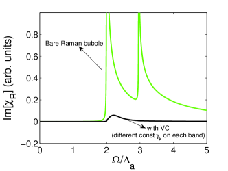
Figure 6: The Raman response of a 2-band $s$-wave SC. The light line is the result when one includes only the bare bubble, dark line is the full result, with vertex corrections(VC) included. These corrections remove the edge singularity and move the peak to a frequency larger than $2\Delta_{\rm min}=\Delta_{a}$. The Raman vertex for each band is chosen to be a constant with $c^{a}_{1}=0.3$ and $c^{b}_{1}=0.2$. Here $V_{a}=-0.2/\nu_{F},~{}V_{b}=-0.3/\nu_{F},~{}V_{3}=0.1/\nu_{F}$, and $\nu_{F,a}=\nu_{F,b}=\nu_{F}$.

$\begin{array}[]{cc}\includegraphics[width=108.405pt]{fig2a}&\includegraphics[width=108.405pt]{fig2b}\\ \includegraphics[width=108.405pt]{fig2c}&\includegraphics[width=108.405pt]{fig2d}\end{array}$

Figure 7: Color online: (a) Solutions to the transcendental Eq. (86) given by the intersection of $\tilde{F}=F/2\nu$ with RHS of Eq. (86) for different $v_{ph}$. (b) The Raman spectrum for $v_{ph}=0,~{}v_{ph}=-0.5\in\{-1/|\tilde{\kappa}|,2\}$, and $v_{ph}=3$ (not in that bound). This case corresponds to the renormalization of the Leggett mode. Here $\tilde{\kappa}=-0.83$. (c) Solutions to the transcendental Eq. 86 and (d) the Raman spectrum for $v_{ph}=0,~{}v_{ph}=1\in\{1/\tilde{\kappa},2\}$, and $v_{ph}=3$ (not in that bound). This shows the emergence of a possible excitonic mode. Here $\tilde{\kappa}=4.2$. Note the removal of the $2\Delta$ edge singularity in all cases.

IV.3.3 Interplay between the Leggett mode and the excitonic mode

To be specific, define $V_{pp}=V_{4}+|V_{3}|$, $V_{ph}=V_{4}-sV_{2}$, and $V_{sc}=V_{4}-|V_{3}|$. We keep $|\Delta^{a}|=|\Delta^{b}|=\Delta$. For $V_{ph}=0$, the Leggett mode necessarily exists at $\Omega<2\Delta$ as long as $V_{pp}<0$ and $V_{sc}<0$ (intra-band attraction-driven superconductivity) and is located at a frequency at which $\Omega^{2}F(\Omega)=2|\kappa|$. In the presence of $V_{ph}$ the zero of the denominator in Eq. (83) shifts to

$$(\Omega^{2}-V_{ph}\kappa)F(\Omega)=-2\kappa$$ (85)

It is convenient to re-express this relation in dimensionless variables $\tilde{F}(\Omega)\equiv F(\Omega)/2\nu_{F}$, $\tilde{\Omega}\equiv\Omega/2\Delta$, $\tilde{\kappa}=\kappa/(4\Delta^{2}\nu_{F})$, and $v_{pp}=V_{pp}\nu_{F}$, etc., and $\tilde{\kappa}=-(v_{pp}-v_{sc}/(v^{2}_{pp}-v^{2}_{sc})$. The locations of the poles are then the roots of the transcendental equation

$$\tilde{F}(\Omega)=\frac{2\tilde{\kappa}}{-\tilde{\Omega}^{2}+v_{ph}\tilde{\kappa}}.$$ (86)

A straightforward analysis shows that when $-1/|\tilde{\kappa}|<v_{ph}<2$, there is one solution at $\tilde{\Omega}<1$: the renormalized Leggett mode. If $v_{ph}$ is outside those bounds, there is no solution on the real frequency axis (see Fig. 7a and b). Now, if $\tilde{\kappa}>0$ and min$\{1/\tilde{\kappa},2\}<v_{ph}<$max$\{1/\tilde{\kappa},2\}$, there is again one solution at $\tilde{\Omega}<1$. This is an excitonic mode (see Fig. 7c and d). When $v_{ph}$ is outside those bounds, there is again no solution on the real frequency axis.

$\begin{array}[]{ccc}\includegraphics[width=140.92517pt]{figb}&\includegraphics[width=140.92517pt]{figc}&\includegraphics[width=140.92517pt]{fige}\end{array}$

Figure 8: The Raman response in the A_1g channel for a 2-band $s-$wave SC. The dashed line is the contribution from the bare bubble. The light red line is the response after accounting for vertex corrections with constant $\gamma_{{\vec{k}}}$: $c^{a}_{1}=1$, $c^{b}_{1}=0.3$. The dark line shows the Raman response for a non-constant $\gamma_{{\vec{k}}}$ where we added $c^{a}_{2}=0.2$, $c^{b}_{2}=0.3$ (corresponding to the $\cos 4\theta$ harmonic). (a) and (b) refer to the case of intra-band driven attractive SC ($V_{a}V_{b}-V_{3}^{2}>0$) and show how the Leggett mode can be pushed to the continuum if $V_{3}$ is increased. (c) is the case of inter-band driven attractive SC ($V_{a}V_{b}-V_{3}^{2}<0$) which has no Leggett mode. Note the removal of $2\Delta$ edge singularity and strong suppression of the spectral weight around $2\Delta$ in all cases. Here $v\equiv V_{3}\nu_{b}$; $\nu_{a}/\nu_{b}=0.6$; and $V_{a}\nu_{b}=-0.5$, $V_{b}\nu_{b}=-0.35$ for (a) and (b); $V_{a}\nu_{b}=0.3$, $V_{b}\nu_{b}=0.6$ for (c). A fermionic lifetime of $0.05\Delta$ is added for broadening.

IV.4 Case of anisotropic two-band system

We now include one more harmonic into $\gamma^{i}({\vec{k}})$ for each band: $\gamma^{a}_{{\vec{k}}}=c^{a}_{1}f^{1}_{{\vec{k}}}+c^{a}_{2}f^{2}_{{\vec{k}}}$, $\gamma^{b}_{{\vec{k}}}=c^{b}_{1}f^{1}_{{\vec{k}}}+c^{b}_{2}f^{2}_{{\vec{k}}}$, and include $V^{aa,22}_{i}$ and $V^{ab,22}_{i}$ harmonics into the interaction. For brevity, we denote $V^{aa,22}_{4}=V^{bb,22}_{4}={\tilde{V}}_{4}$, $V^{ab,22}_{2}={\tilde{V}}_{2}$, and $V^{ab,22}_{3}={\tilde{V}}_{3}$. The $[V]$, $[\Pi]$ and $[c]$ matrices in this case are:

$$[V_{pp}]=\left(\begin{array}[]{cccc}V_{4}&V_{3}&0&0\\ V_{3}&V_{4}&0&0\\ 0&0&\tilde{V}_{4}&\tilde{V}_{3}\\ 0&0&\tilde{V}_{3}&\tilde{V}_{4}\\ \end{array}\right)\otimes\sigma_{0};~{}[V_{ph}]=\left(\begin{array}[]{cccc}V_{4}&V_{2}&0&0\\ V_{2}&V_{4}&0&0\\ 0&0&\tilde{V}_{4}&\tilde{V}_{2}\\ 0&0&\tilde{V}_{2}&\tilde{V}_{4}\\ \end{array}\right)\otimes\sigma_{0};$$ (87)

and $[c]^{T}=(0,c_{1}^{a},0,c_{1}^{b},0,c_{2}^{a},0,c_{2}^{b})$. Following usual steps we obtain,

$$\chi_{R}(\Omega) = \frac{(c_{1}^{a}-c_{1}^{b})^{2}}{2}\left[\frac{\Pi_{33}-\frac{(\Pi_{23})^{2}}{\frac{2}{V_{4}+|V_{3}|}-\Pi_{22}}}{1+\frac{V_{4}-sV_{2}}{2}\left(\Pi_{33}-\frac{(\Pi_{23})^{2}}{\frac{2}{V_{4}+|V_{3}|}-\Pi_{22}}\right)}\right]$$

$$+\frac{(c_{2}^{a}+c_{2}^{b})^{2}}{2}\left[\frac{\Pi_{33}-\frac{(\Pi_{23})^{2}}{\frac{2}{\tilde{V}_{4}-s\tilde{V}_{3}}-\Pi_{22}}}{1+\frac{\tilde{V}_{4}+s\tilde{V}_{2}}{2}\left(\Pi_{33}-\frac{(\Pi_{23})^{2}}{\frac{2}{\tilde{V}_{4}-s\tilde{V}_{3}}-\Pi_{22}}\right)}\right]+\frac{(c_{2}^{a}-c_{2}^{b})^{2}}{2}\left[\frac{\Pi_{33}-\frac{(\Pi_{23})^{2}}{\frac{2}{\tilde{V}_{4}+s\tilde{V}_{3}}-\Pi_{22}}}{1+\frac{\tilde{V}_{4}-s\tilde{V}_{2}}{2}\left(\Pi_{33}-\frac{(\Pi_{23})^{2}}{\frac{2}{\tilde{V}_{4}+s\tilde{V}_{3}}-\Pi_{22}}\right)}\right].$$

The particle conservation does not impose restrictions in the $c_{2}$ channel, hence both terms in the second line in Eq. (IV.4) are generally non-zero. There may be additional resonances in $\chi_{R}(\Omega)$ due to poles in these two terms. It is essential to note that each term in Eq. (IV.4) still vanishes at $\Omega=2\Delta$, i.e., the divergence in Im[$\Pi_{33}$] at $\Omega=2\Delta+0$ is eliminated by vertex corrections. In practice, higher harmonics are more likely to just add the spectral weight to the $2\Delta$ Raman continuum rather than induce new resonances below $2\Delta$ (see Fig. 8).

V Role of Coulomb interaction

We now move to include the effects of Coulomb interaction into the A_1g response. It was argued in the past that screening from the long-range Coulomb interaction is a necessary ingredient of Raman analysis, and that this screening accounts for the vanishing of the Raman susceptibility in the case when Raman vertex $\gamma^{a}({\vec{k}})$ can be treated as a constant, independent of the band index. We have now shown that vertex corrections already account for the vanishing of $\chi_{R}(\Omega)$ in this situation. We now argue that, at ${\vec{q}}\to 0$, the Coulomb interaction does not affect the Raman susceptibility for an arbitrary Raman vertex $\gamma^{a}({\vec{k}})$. Namely, we argue that both $\pi_{CR}(=\pi_{RC})$ and $\pi_{CC}$ vanish, no matter what $\gamma^{a}({\vec{k}})$ is and thus there is no screening correction to the Raman response in a SC when $q\rightarrow 0$.

For non-A_1g scattering geometry, the vanishing of $\pi_{RC,CR}$ is obvious because non-s-wave eigenfunctions and a constant charge form-factor are orthogonal. For s-wave scattering and $\gamma^{a}({\vec{k}})$ = const it is also obvious because then $\pi_{RC,CR}=\pi_{RR}=\pi_{CC}$, and all vanish for $q\to 0$. However, it is less obvious when the scattering is in s-wave geometry (e.g., $A_{1g}$ geometry for a 2D quare lattice), but $\gamma^{a}({\vec{k}})$ has momentum-dependent harmonics, or has momentum-independent, but different values, for different bands.

The logical reasoning for the vanishing of $\pi_{RC,CR}$ in this case is the following. The screening correction is given by $\pi_{RC}\pi_{CR}/[1/V_{C}({\vec{q}})-\pi_{CC}]$. The quantity $\pi_{CC}$ is a fully renormalized density-density correlator, and it vanishes at $q=0$ (as we just demonstrated for the Raman bubble in case when $\gamma^{a}({\vec{k}})$ = const. One can easily extend that analysis to finite $q$ and show that at $v_{F}q\ll\Omega$, $\pi_{CC}\propto q^{2}(\Omega_{\rm pl}/\Omega)^{2}$, where $\Omega_{\rm pl}$ is the plasma frequency. This holds both in the normal state and in the SC state. The obvious consequence is that $1/V_{C}({\vec{q}})-\pi_{CC}=0$ at the plasma frequency in 3D and at $\Omega\propto\sqrt{q}$ in 2D. Because in both cases $1/V_{C}({\vec{q}})-\pi_{CC}$ vanishes at $q=0$, the screening correction would have an unphysical divergent contribution to the Raman response if $\pi_{RC,CR}$ were non-zero at $q=0$. The requirement that the theory must be free from divergencies then forces $\pi_{RC,CR}(q=0)$ to vanish. The expansion of a charge response function in $q$ in necessarily analytic,maslov hence $\pi_{RC,CR}(q)\propto q^{2}$. Then the contribution to $R(\Omega)$ from Coulomb screening scales as $q^{2}$ in 3D and as $q^{3}$ in 2D and vanishes at $q\to 0$.

Below we demonstrate that $\pi_{RC,CR}(q=0)=0$ for the two non-trivial cases – a two-band superconductor with different momentum-independent $\gamma^{a}$ for the two bands and a one-band superconductor with an anisotropic s-wave gap and arbitrary $\gamma({\vec{k}})$ for s-wave scattering.

V.1 Absence of screening in a two-band SC with isotropic gap

The generic expression for $\pi_{RC}(Q)$ is given by Eq. (11), where, we remind the reader, $\bar{\Gamma}^{a}$ is the fully renormalized charge vertex, with partial components ${\bar{\Gamma}}^{a,t}_{2}$ and ${\bar{\Gamma}}^{a,t}_{3}$. Because we assume the Raman vertex to be momentum-independent, only partial components with $t=1$ are non-zero.

To show that $\pi_{RC}(q=0)$ vanishes, we follow the same strategy as for the analysis of $\pi_{RR}$ and first include only the renormalizations in the particle-particle channel, i.e., neglect terms with $\Pi^{aa,11}_{32},\Pi^{aa,11}_{33},\Pi^{bb,11}_{32}$ and $\Pi^{bb,11}_{33}$ (we call the corresponding piece $\pi^{pp}_{RC}$. From Eq. (11) we then obtain

$$\pi^{pp}_{RC}(q=0) = c^{a}_{1}\left[\Pi^{aa,11}_{33}\bar{\Gamma}^{a,1}_{3}+\Pi^{aa,11}_{32}\bar{\Gamma}^{a,1}_{2}\right]$$ (89)

$$+c^{b}_{1}\left[\Pi^{bb,11}_{33}\bar{\Gamma}^{b,1}_{2}+\Pi^{bb,11}_{32}\bar{\Gamma}^{b,1}_{2}\right]$$

Evaluating $\Pi^{aa,11}_{32}(\Omega)$ and $\Pi^{aa,11}_{33}(\Omega)$, we find that they are related:

$$\Pi^{aa,11}_{32}(\Omega)=\frac{i\Omega}{2\Delta^{a}}\Pi^{aa,11}_{33}(\Omega)$$ (90)

The same relation holds for the $b-$band

$$\Pi^{bb,11}_{32}(\Omega)=\frac{i\Omega}{2\Delta^{b}}\Pi^{bb,11}_{33}(\Omega)$$ (91)

Substituting these relations into Eq. (89), we obtain

$$\pi^{pp}_{RC}(q=0) = c^{a}_{1}\Pi^{aa,11}_{33}\left[\bar{\Gamma}^{a,1}_{3}+(i\Omega/2\Delta^{a})\bar{\Gamma}^{a,1}_{2}\right]$$ (92)

$$+c^{b}_{1}\Pi^{bb,11}_{33}\left[\bar{\Gamma}^{b,1}_{3}+(i\Omega/2\Delta^{b})\bar{\Gamma}^{b,1}_{2}\right]$$

Now, from the last two lines in Eq. (21) and Eq. (III) we obtain for ${\bar{\Gamma}}$:

$$\bar{\Gamma}^{a,1}_{3} = 1$$

$$\bar{\Gamma}^{a}_{2,1} = \frac{2V_{3}\Pi^{bb,11}_{23}-\Pi^{aa,11}_{23}\left\{V_{a}\left(-2+V_{b}\Pi^{bb,11}_{22}\right)-\Pi^{bb,11}_{22}V_{3}^{2}\right\}}{4\mathcal{D}}$$ (93)

$$= -\frac{2\Delta^{a}}{i\Omega},$$

$$\bar{\Gamma}^{b,1}_{3} = 1$$

$$\bar{\Gamma}^{b,1}_{2} = \frac{2V_{3}\Pi^{aa,11}_{23}-\Pi^{bb,11}_{23}\left\{V_{b}\left(-2+V_{a}\Pi^{aa}_{22}\right)-\Pi^{aa,11}_{22}V_{3}^{2}\right\}}{4\mathcal{D}}$$

$$= -\frac{2\Delta^{b}}{i\Omega}$$

Substituting into Eq. (92) we see that each term in Eq. (92) vanishes. Then $\pi^{pp}_{RC}(q=0)=0$ for arbitrary $c^{a}_{1}$ and $c^{b}_{1}$.

The analysis can be straightforwardly extended to include the renormalizations in the particle-hole channel. We indeed found that the result holds, i.e., $\pi_{RC}(q=0)=0$. We do not show the details of the proof as the calculations are somewhat lengthy.

V.2 Absence of screening in a one-band SC with anisotropic gap and arbitrary $\gamma({\vec{k}})$

To be specific, consider a 2D SC on a square lattice and assume that the interaction is only in the pairing channel and is in the form $V_{pp}({\vec{k}},{\vec{k}}^{\prime})=Vf_{{\vec{k}}}f_{{\vec{k}}^{\prime}}$, where $f_{{\vec{k}}}=1+r\cos 4\theta+...$. We assign the index $f$ to this harmonic (i.e., set $f_{{\vec{k}}}\equiv f^{f}_{{\vec{k}}}$) and the index 1 to $f^{1}_{{\vec{k}}}=1$. For such $V_{pp}$, the pairing gap has the form $\Delta({\vec{k}})=\Delta_{0}f_{{\vec{k}}}$. Using Eq. (21), one can easily check that in this situation $\bar{\Gamma}_{3}=1$ because, the renormalization of ${\bar{\Gamma}}_{3}$ could only come from the interaction in the particle-hole channel. Further, $\bar{\Gamma}_{2}({\vec{k}})=\sum_{t}\bar{\Gamma}^{t}_{2}({\vec{k}})f^{t}_{{\vec{k}}}$ has only the harmonic with the index f, i.e., $\bar{\Gamma}_{2}({\vec{k}})={\bar{\Gamma}}_{2}f_{{\vec{k}}}$. Substituting the last form into Eq. (21) we obtain, skipping the band index,

$$\bar{\Gamma}_{2} = \frac{V}{2}\Pi^{ff}_{22}\bar{\Gamma}_{2}+\frac{V}{2}\Pi^{f1}_{23}$$ (94)

Hence

$$\bar{\Gamma}_{2} = \frac{\Pi^{f1}_{23}}{\frac{2}{V}-\Pi^{ff}_{22}}.$$ (95)

From Eq. (12) we then obtain, for arbitrary $\gamma({\vec{k}})=\sum_{t}c_{t}f^{t}_{{\vec{k}}}$

$$\pi_{RC}(\Omega) = \sum_{t}c_{t}\int_{K^{\prime}}f^{t}_{{\vec{k}}^{\prime}}f_{{\vec{k}}^{\prime}}\text{Tr}[\sigma_{3}G_{K^{\prime}}\sigma_{2}G_{K^{\prime}+Q}]\bar{\Gamma}_{2}$$ (96)

$$+\sum_{t}c_{t}\int_{K^{\prime}}f^{t}_{{\vec{k}}^{\prime}}\text{Tr}[\sigma_{3}G_{K^{\prime}}\sigma_{3}G_{K^{\prime}+Q}]$$

$$\equiv \sum_{t}c_{t}\left(\Pi^{tf}_{32}\bar{\Gamma}_{2}+\Pi^{t1}_{33}\right).$$

On explicitly evaluating the polarization operators $\Pi^{ff}_{22},\Pi^{f1}_{23},\Pi^{tf}_{32}$, and $\Pi^{t1}_{33}$, we obtain

$$\Pi^{f1}_{23} = \frac{i\Omega}{2\Delta_{0}}F^{ff}(\Omega);$$

$$\Pi^{tf}_{32} = -\frac{i\Omega}{2\Delta_{0}}\tilde{F}^{tf}(\Omega);$$

$$\Pi^{t1}_{33} = -\tilde{F}^{tf}(\Omega);$$

$$\Pi^{ff}_{22} = \frac{2}{V}-\left(\frac{\Omega}{2\Delta_{0}}\right)^{2}F^{ff}(\Omega),$$ (97)

where $F^{ff}(\Omega)\equiv\int_{{\vec{k}}}\Delta_{0}^{2}f^{2}_{{\vec{k}}}/4E[E^{2}-(\Omega/2)^{2}]$ and $\tilde{F}^{tf}(\Omega)\equiv\int_{{\vec{k}}}\Delta_{0}^{2}f^{t}f^{2}_{{\vec{k}}}/4E[E^{2}-(\Omega/2)^{2}]$. Observe that

$$\Pi^{tf}_{32}=\frac{i\Omega}{2\Delta_{0}}\Pi^{t1}_{33}.$$ (98)

Using the last relation we re-express $\pi_{RC}$ from Eq. (96) as

$$\pi_{RC}(\Omega)=\sum_{t}c^{t}\Pi^{t1}_{33}\left[1+\frac{i\Omega}{2\Delta_{0}}\bar{\Gamma}_{2}\right].$$ (99)

Using Eqs. (95) and (V.2) we then find that

$$\bar{\Gamma}_{2}=-\frac{2\Delta_{0}}{i\Omega}.$$ (100)

Substituting this result in Eq. (99) we see each term under the sum over $t$ vanishes. As the consequence, $\pi_{RC}(\Omega)=0$ for any $\gamma_{{\vec{k}}}$.

VI Non-A_1g channels

Finally we briefly discuss the spectrum in non-A_1g channels and highlight their appealing aspects for the experiments. To get there, let us note that the common features of the Raman response across all A_1g and non-A_1g channels are: (1) removal of the $2\Delta$ edge singularity and (2) presence of collective modes under favorable conditions. What is different is that in A_1g scattering geometry one always probes fluctuations in the pairing channel with the symmetry of the pairing gap, whereas in the non-A_1g scattering geometry one probe fluctuations in subleading channels, where interaction may be attractive (but weaker than in the leading channel). For example, in an $s-$wave SC Raman intensity in A_1g scattering geometry may have sharp peaks corresponding to Leggett modes, which represent fluctuations of the relative phases of the multi-component order parameters, while Raman intensity in B_1g scattering geometry may have peaks corresponding to BS modes if a subleading $d-$wave channel is attractive.

It is also easy to see that in a $d$-wave SC, it is the Raman scattering in A_1g geometry that is strongly affected by vertex corrections. Indeed, to convert from a particle-hole to a particle-particle channel, one needs a combination of a normal and an anomalous Green’s function. The anomalous Green’s function has $\Delta({\vec{k}})$ in the numerator. Hence, for A_1g scattering geometry, the resulting form-factor for particle-particle channel has a $d-$wave symmetry. Then one needs $d-$wave pairing interaction (the same that leads to SC) to renormalize it. In other words, the fluctuations of a $d-$wave SC order parameter are probed in Raman experiments in an A_1g scattering geometry. And vise versa - the Raman response in a B_1g scattering geometry in a $d$-wave SC probes pairing fluctuations in $s-$wave channel.

VII Conclusion

To conclude, we have presented the general scheme to calculate the Raman response in a multi-band superconductor with both short-range and long-range interactions between fermions. We grouped the interactions into the screening part and the part which accounts for the renormalizations of the Raman vertex. We further decomposed vertex renormalizations into those in the particle-particle and in the particle-hole channels. The renormalizations in the particle-particle channel are unavoidable in a superconductor because a particle-hole Raman vertex can be converted into particle-particle vertex via the renormalization which involves one normal and one anomalous fermionic Green’s function ($\Pi_{23}$ polarization bubble in the Nambu formalism). We have presented a general formula that accounts for vertex corrections in particle-particle and particle-hole channels in a generic multi-band superconductor. We demonstrated that vertex corrections in the particle-particle channel cannot be neglected as they enforce the constraint imposed by the particle number conservation. This point has been emphasized in Ref. [Lara, ], and our results are in agreement with theirs.

We argued that in a situation when the Raman form-factor ($\gamma_{{\vec{k}}}$) is momentum-independent and the same for all bands, vertex corrections completely eliminate the Raman response. For a generic polarizations of light Raman intensity remains finite, but vertex corrections remove the $2\Delta$ edge singularity of the bare bubble, leaving only a broad maximum at a frequency above $2\Delta$. Besides, vertex corrections account for $\delta-$function contributions to the Raman intensity from collective modes, at frequencies below twice the minimum gap. Specifically, we analyzed the contributions to $A_{1g}$ Raman intensity of a 2D system on a square lattice from the Leggett mode in the particle-particle channel and the excitonic mode in the particle-hole channel, and the interplay between the two.

We also demonstrated that, once vertex corrections inside the Raman bubble are included, the remaining RPA-type renormalizations of the Raman susceptibility by long-range Coulomb interaction (screening corrections) are negligibly small at $q\to 0$, even for the A_1g scattering geometry on a lattice when $s-$wave Raman form-factor has some momentum dependence. This implies that long-range Coulomb interaction is irrelevant for the Raman scattering when $q\rightarrow 0$.

The formalism that we developed applies to any pairing symmetry, any number of bands, and a generic form of the Raman vertex $\gamma({\vec{k}})$. It can also be easily extended to tackle time-reversal symmetry broken superconducting states, like $s+is$,SM_AVC ; Benfatto ; spisLegget1 ; spisLegett2 $s+id$,Hanke etc.. The temperature dependence of the energies of the collective modes can also be inferred from Raman experiments. To obtain it theoretically, one needs to keep temperature dependence in the polarization operators $\Pi^{aa,mn}_{ij}$.

Acknowledgements. We thank G. Blumberg, L. Benfatto, T. Devereaux, D. Einzel, R. Hackl, and D. Maslov for useful discussions. We are also thankful to L. Benfatto and R. Hackl and R. Hackl for comments on the manuscript. This work was supported by the Office of Basic Energy Sciences, U.S. Department of Energy, under awards DE-SC0014402 (AVC) and DE-FG02-05ER46236 (PJH). AVC thanks the Perimeter Institute for Theoretical Physics (Waterloo, Canada) for hospitality during the final stages of this project. The research at the Perimeter Institute is supported in part by the Government of Canada through the Department of Innovation, Science and Economic Development and by the Province of Ontario through the Ministry of Research and Innovation.

References

- (1) B. S. Shastry and B. I. Shraiman, Phys. Rev. Lett. 65, 1068 (1990).
- (2) T. P. Devereaux and R. Hackl, Rev. Mod. Phys. 79, 175 (2007).
- (3) A. J. Leggett, Prog. Theor. Phys. 36, 901 (1966).
- (4) A. Bardasis and J. R. Schrieffer, Phys. Rev. 121, 1050 (1961).
- (5) V. G. Vaks, V. M. Galitskii, and A. I. Larkin, Zh. Eksp. Teor. Fiz. 41, 1655 (1961) [Sov. Phys.—JETP 14, 1177 (1962)].
- (6) H. Monien and A. Zawadowski Phys. Rev. B 41, 8798 (1990).
- (7) A. Chubukov and P. J. Hirschfeld, Phys. Today 68, No. 6, 46 (2015).
- (8) P. J. Hirschfeld, C.R. Phys. 17, 197 (2016).
- (9) G. Blumberg, A. Mialitsin, B. S. Dennis, M. V. Klein, N. D. Zhigadlo, and J. Karpinski, Phys. Rev. Lett. 99, 227002 (2007).
- (10) M. V. Klein, Phys. Rev. B 82, 014507 (2010).
- (11) F. Kretzschmar, B. Muschler, T. Bohm, A. Baum, R. Hackl, Hai-Hu Wen, V. Tsurkan, J. Deisenhofer, and A. Loidl, Phys. Rev. Lett. 110, 187002 (2013).
- (12) T. Bohm, A. F. Kemper, B. Moritz, F. Kretzschmar, B. Muschler, H.-M. Eiter, R. Hackl, T.P. Devereaux, D. J. Scalapino, and H.-H.Wen Phys. Rev. X 4, 041046 (2014).
- (13) V. K. Thorsmolle, M. Khodas, Z. P. Yin, Chenglin Zhang, S. V. Carr, Pengcheng Dai, G. Blumberg, arXiv:1410.6456 (2014).
- (14) T. Cea, L. Benfatto, Phys. Rev. B 90, 224515 (2014).
- (15) T. Cea, C. Castellani, G. Seibold, L. Benfatto, Phys. Rev. Lett. 115, 157002 (2015).
- (16) T. Cea, C. Castellani, L. Benfatto, Phys. Rev. B 93, 180507 (2016).
- (17) S.-Z. Lin and X. Hu Phys. Rev. Lett. 108, 177005 (2012).
- (18) V. Stanev Phys. Rev. B 85 174520 (2012).
- (19) S. Maiti and A. V. Chubukov, Phys. Rev. B 87, 144511 (2013).
- (20) M. Marciani, L. Fanfarillo, C. Castellani, and L. Benfatto, Phys. Rev. B 88, 214508 (2013).
- (21) P. B. Littlewood and C. M. Varma, Phys. Rev. B 26, 4883, (1982).
- (22) S. A. Weidinger, W. Zwerger, Eur. Phys. Jour. B 88, 237(2015).
- (23) A.A. Abrikosov and V.M. Genkin, JETP 38, 417(1974).
- (24) M. V. Klein and S. B. Dierker, Phys. Rev. B 29, 4976, (1984).
- (25) A.A. Abrikosov and Fal’kovsky, Physica C, 156, 1 (1988).
- (26) W.-C. Wu and A. Griffin, Phys. Rev. B, 51, 1190 (1995).
- (27) T. P. Devereaux, D. Einzel, B. Stadlober, R. Hackl, D. H. Leach, and J. J. Neumeier Phys. Rev. Lett. 72, 396 (1994); T. P. Devereaux and D. Einzel Phys. Rev. B 51, 16336 (1995).
- (28) G. R. Boyd, T. P. Devereaux, P. J. Hirschfeld, V. Mishra, and D. J. Scalapino, Phys. Rev. B 79, 174521 (2009).
- (29) T. Cea, L. Benfatto Phys. Rev. B 94, 064512 (2016).
- (30) C. Sauer and G. Blumberg, Phys Rev B, 82, 014525 (2010).
- (31) T. P. Devereaux, A. Virosztek, and A. Zawadowski Phys. Rev. B 54, 12523 (1996).
- (32) A. V. Chubukov, I. Eremin, M. M. Korshunov, Phys. Rev. B 79, 220501(R) (2009).
- (33) D. J. Scalapino and T. P. Devereaux, Phys. Rev. B 80, 140512 (2009).
- (34) M. Khodas, A.V. Chubukov, G. Blumberg, Phys. Rev. B 89, 245134 (2014).
- (35) S. Maiti, T. Maier, T. Böhm, R. Hackl, P. Hirschfeld, Phys. Rev. Lett. 117, 257001 (2016).
- (36) http://mathworld.wolfram.com/KroneckerProduct.html
- (37) A.V. Chubukov, Physica C 469, 640 (2009).
- (38) A. V. Chubukov, D. V. Efremov, and I. Eremin, Phys. Rev. B 78, 134512 (2008).
- (39) S. Maiti and A. V. Chubukov, Phys. Rev. B 82, 214515 (2010).
- (40) D.Einzel, N. Bittner, unpublished.
- (41) S. Maiti, P. Hirschfeld, Phys. Rev. B. 92, 094506(2015).
- (42) A. Hinojosa, J. Cai, and A. V. Chubukov, Phys. Rev. B 93, 075106 (2016).
- (43) We only retain intraband wave interaction to reduce the number of parameters.
- (44) C. Platt, R. Thomale, C. Honerkamp, S.-C. Zhang, and W. Hanke, Phys. Rev. B 85, 180502(R) (2012).
- (45) A.V. Chubukov and D.L. Maslov, Phys. Rev. B68, 155113 (2003); D. Belitz, T.R. Kirkpatrick, and T. Vojta, Rev. Mod. Phys. 77, 579 (2005).