Computationally Efficient Simulation of Queues: The R Package queuecomputer

queuecomputer: Computationally Efficient Simulation of Queues Anthony Ebert, Paul Wu, Kerrie Mengersen, Fabrizio Ruggeri Computationally Efficient Simulation of Queues: The R Package queuecomputer Large networks of queueing systems model important real-world systems such as MapReduce clusters, web-servers, hospitals, call centers and airport passenger terminals. To model such systems accurately, we must infer queueing parameters from data. Unfortunately, for many queueing networks there is no clear way to proceed with parameter inference from data. Approximate Bayesian computation could offer a straightforward way to infer parameters for such networks if we could simulate data quickly enough. We present a computationally efficient method for simulating from a very general set of queueing networks with the R package queuecomputer. Remarkable speedups of more than 2 orders of magnitude are observed relative to the popular DES packages simmer and simpy. We replicate output from these packages to validate the package. The package is modular and integrates well with the popular R package dplyr. Complex queueing networks with tandem, parallel and fork/join topologies can easily be built with these two packages together. We show how to use this package with two examples: a call center and an airport terminal. queues, queueing theory, discrete event simulation, operations research, approximate Bayesian computation, R queues, queueing theory, discrete event simulation, operations research, approximate Bayesian computation, R Anthony Ebert
School of Mathematical Sciences
Science and Engineering Faculty
Queensland University of Technology
Brisbane Queensland 4000, Australia
E-mail:
URL: https://acems.org.au/our-people/anthony-ebert

1 Introduction

The queues we encounter in our everyday experience, where customers wait in line to be served by a server, are a useful analogy for many other processes. We say analogy because the word customers could represent: MapReduce jobs (lin_joint_2013); patients in a hospital (takagi_queueing_2016); items in a manufacturing system (dallery_manufacturing_1992); calls to a call center (gans_telephone_2003); shipping containers in a seaport (kozan_comparison_1997) or even cognitive tasks (cao_queueing_2013). Similarly, server could represent: a compute cluster; medical staff; machinery or a customer service representative at a call center. Queueing systems can also be networked together to form queueing networks. We can use queueing networks to build models of processes such as provision of internet services (sutton_bayesian_2011), passenger facilitation at international airports (wu_review_2013) and emergency evacuations (van_woensel_modeling_2007). Clearly queueing systems and queueing networks are useful for understanding important real-world systems.

Performance measures for a given queueing system can often only be derived through simulation. Queues are usually simulated with discrete event simulation (DES) (insua2012bayesian, pg. 226). In DES changes in state are discontinuous. The state is acted upon by a countable list of events at certain times which cause the discontinuities. If the occurrence of an event is independent of everything except simulation time it is determined; otherwise, it is contingent (nance1981time).

Popular DES software packages are available in many programming languages including: the R package simmer (Rpkg_simmer), the Python (van2011python) package simpy (Ppkg_simpy) and the Java (gosling2000java) package JMT (Jpkg_JMT). DES packages are often so expressive that they can be considered languages in their own right, indeed the programming language Simula (dahl1966simula) is a literal example of this.

queuecomputer (Rpkg_queuecomputer) implements an algorithm that can easily be applied to a wide range of queueing systems and networks of queueing systems. It is vastly more computationally efficient than existing approaches to DES. We term this new computationally efficient algorithm queue departure computation (QDC). Computational efficiency is important because if we can simulate from queues quickly, then we can embed a queue simulation within an approximate Bayesian computation (ABC) algorithm (sunnaker_approximate_2013) and estimate queue parameters for very complicated queueing models in a straightforward manner.

In Section 2 we review the literature on queueing theory and develop notation used throughout this paper. In Section 3 we present the QDC algorithm and compare it to DES. We demonstrate usage of the package in Section 4. Details of implementation and usage are discussed in Section 5. The package is validated in Section 6 by replicating results from DES packages simpy and simmer. We compare computed performance measures from the output of a queuecomputer simulation to theoretical results for $M/M/2$ queueing systems. We benchmark the package in Section 7 and compare computation time with simpy and simmer. Examples in Section 8 are used to demonstrate how the package can be used to simulate a call center and an international airport terminal.

2 Queueing theory

Queueing theory is the study of queueing systems and originated from the work of Agner Krarup Erlang in 1909 to plan infrastructure requirements for the Danish telephone system (thomopoulos2012fundamentals, pg 2).

A queueing system is defined as follows. Each customer $i=1,2,\cdots$ has an arrival time $a_{i}$ (or equivalently an inter-arrival time $\delta_{i}=a_{i}-a_{i-1}$, $a_{0}=0$) and an amount of time they require with a server, called the service time $s_{i}$. Typically a server can serve only one customer at a time. A server which is currently serving another customer is said to be unavailable, a server without a customer is available. If all servers are unavailable when a customer arrives then customers must wait in the queue until a server is available. Detailed introductions to queueing systems can be found in standard texts such as bhat2015introduction.

The characteristics of a queueing system are expressed with the notation of kendall1953stochastic. This notation has since been extended to six characteristics:

• $f_{\mathbf{\delta}}$, inter-arrival distribution;

• $f_{\mathbf{s}}$, service distribution;

• $K$, number of servers $\in\mathbb{N}$;

• $C$, capacity of system $\in\mathbb{N}$;

• $n$, customer population $\in\mathbb{N}$; and

• $R$, service discipline

Choices for inter-arrival and service distributions are denoted by “M" for exponential and independently distributed, “GI" for general and independently distributed and “G" for general without the independence assumption. The capacity of the system $C$ refers to the maximum number of customers within the system at any one time. Customers are within the system if they are being served or waiting in the queue. The customer population $n$ is the total number of customers including those outside of the system (yet to arrive or already departed). The service discipline $R$ defines how customers in the queue are allocated to available servers. The most common service discipline is first come first serve (FCFS). To specify a queueing system, these characteristics are placed in the order given above and separated by a forward slash “/".

The simplest queueing system is exponential in distribution for both the inter-arrival $\delta_{i}\overset{iid}{\sim}\mathrm{exp}(\lambda)~{}\forall i\in 1:n$ and service processes $s_{i}\overset{iid}{\sim}\mathrm{exp}(\mu)~{}\forall i\in 1:n$, where $\lambda$ and $\mu$ are exponential rate parameters. Additionally, $K$ is set to 1, $C$ and $n$ are infinite, and $R$ is FCFS. It is denoted by $M/M/1/\infty/\infty/FCFS$, which is shortened to $M/M/1$.

Parameter inference for this system was considered first by clarke1957maximum, estimators were derived from the likelihood function. This likelihood is later used by muddapur1972bayesian to derive the joint posterior distribution. Bayesian inference for queueing systems is summarised in detail by insua2012bayesian.

Managers and planners are less interested in parameter inference and more interested in performance measures such as: $N(t)$, the number of customers in system at time $t$; $\bar{B}$, the average number of busy servers; $\rho$, the resource utilization; and $\bar{\mathbf{w}}$, the average waiting time for customers. If $\lambda<K\mu$ the queueing system will eventually reach equilibrium and distributions of performance measures become independent of time.

In the case of a $M/M/K$ system equilibrium distributions for performance measures are derived analytically, they are found in standard queueing theory textbooks (lipsky2008queueing; thomopoulos2012fundamentals). For instance, the limit probability of $N$ customers in the system $\Prob(N)$ is

$$\Prob(0) =\left[\frac{(K\rho)^{K}}{K!(1-\rho)}+1+\sum_{i=1}^{K-1}\frac{(K\rho)^{i}}{i!}\right]^{-1}$$

$$\Prob(N) =\begin{cases}\Prob(0)\frac{(K\rho)^{n}}{N!}&\quad N\leq K\\ \Prob(0)\frac{(K\rho)^{n}}{K!K^{N-K}}&\text{otherwise}\end{cases}$$ (1)

where $\rho$, the resource utilization, is defined as $\frac{\lambda}{K\mu}$. For an $M/M/K$ system this is equal to the expected number of busy servers divided by the total number of servers $\frac{\E(B)}{K}$ (cassandras2009introduction, pg. 451). The expected number of customers in the system is (bhat2015introduction)

$$\E(N)=K\rho+\frac{\rho(K\rho)^{K}P(0)}{K!(1-\rho)^{2}},$$ (2)

and the expected waiting time is

$$\E(\mathbf{w})=\frac{(K\rho)^{K}P(0)}{K!K\mu(1-\rho)^{2}}.$$ (3)

If the parameters of $f_{\delta}$ and $f_{\mathbf{s}}$ are uncertain, then we must turn to predictive distributions for estimates of performance measures, which are computed analytically for M/M/K queues (Equations 2 and 3). Predictive distributions of performance measures using Bayesian posterior distributions are derived by armero1994bayesian; armero1999dealing.

jackson_networks_1957 was one of the first to consider networks of queueing systems. In a Jackson network, there is a set of $J$ queueing systems. After a customer is served by queueing system $j$, they arrive at another queueing system with fixed probability $p_{j,k}$. Customers leave the system with probability $1-\sum_{k=1}^{J}p_{j,k}$. Other examples of queueing networks include the tandem (glynn_departures_1991), parallel (hunt_fast_1995) and the fork/join (kim_analysis_1989) topologies.

In a tandem queueing network, customers traverse an ordered series of queues before departing the system. Real examples of such systems include airport terminals, internet services and manufacturing systems. In a parallel network, customers are partitioned into different $\mathbf{(a,s)}$ to be seen by separate queueing systems. In a fork/join network a task (another term for customer) is forked into a number of subtasks which are to be completed by distinct parallel servers. The difference from the parallel network is that the task can only depart the system once all subtasks have arrived at the join point.

Most models of queueing systems assume time-invariant inter-arrival and service processes. In practice, many real-world queues have inter-arrival processes which are strongly time-dependent, such as: call centers (weinberg2007bayesian; brown2005statistical), airport runways (koopman1972air) and hospitals (brahimi_queueing_1991). In the case of the $M/M/1$ queue, we can adapt the notation to $M(t)/M(t)/1$ to represent exponential processes where parameters $\lambda(t)$ and $\mu(t)$ change with time. Such queueing systems are referred to as dynamic queueing systems.

In general, analytic solutions do not exist for dynamic queueing systems (malone1995dynamic; worthington2009reflections). green1991some showed that using stationary queueing systems to model dynamic queueing systems leads to serious error even if deviation from stationarity is slight. The problem is compounded once we consider queueing networks. Understanding long-term and transient behaviour of such queues can only be achieved with approximation methods or simulation. We now detail the QDC algorithm, a computationally efficient method for simulating queueing systems.

3 Queue departure computation

3.1 Fixed number of servers

QDC can be considered as a multiserver extension to an algorithm presented by lindley_theory_1952. For a single server queueing system, the departure time of the $i$th customer is: $d_{i}=\max{(a_{i},d_{i-1})}+s_{i}$, since the customer either waits for a server or the server waits for a customer. The algorithm (not the paper) was, surprisingly, not extended to multiserver systems until krivulin_recursive_1994. However with each new customer $i$ the algorithm must search a growing $i+1$ length vector. This algorithm, therefore, scales poorly, with computational complexity $O(n^{2})$, where $n$ is number of customers. kin_generalized_2010 adapted the original algorithm of kiefer_theory_1955 to an $O(nK)$ algorithm for multiserver tandem queues with blocking, that is $G/G/K/C$ queueing systems where $C$ is the maximum capacity number of customers in the queueing systems.

QDC can also be viewed as a computationally efficient solution to the set of equations presented in sutton_bayesian_2011 for FCFS queueing systems. There is a single queue served by a fixed number of $K$ servers. The $i$th customer observes a set of times $b_{i}=\{b_{ik}|k\in 1:K\}$ which represents the times when each server will next be available. The customer $i$ selects the earliest available server $p_{i}=\text{argmin}(b_{i})$ from $b_{i}$. The departure time for the $i$th customer is, therefore, $d_{i}=\max({a_{i},b_{p_{i}}})+s_{i}$, since the server must wait for the customer or the customer must wait for the server. The QDC algorithm for a fixed number of servers (Algorithm 1) pre-sorts the arrival times. Rather than assigning a $b_{i}$ for each customer $i$ to form the matrix $\mathbf{b}\in\mathbf{M}^{n\times K}$, QDC considers $\mathbf{b}$ as a continually updated $K$ length vector representing the state of the system.

Algorithm 1 QDC for fixed $K$

1:function QDC_numeric($\mathbf{a}\in\mathbb{R}_{+}^{n},\mathbf{s}\in\mathbb{R}_{+}^{n},K\in\mathbb{N}$)

2:     Sort $(\mathbf{a},\mathbf{s})$ in terms of $\mathbf{a}$ (ascending)

3:     Create vector $\mathbf{p}\in\mathbb{N}^{n}$.

4:     Create vector $\mathbf{b}\in\mathbb{R}_{+}^{K}$.

5:     Create vector $\mathbf{d}\in\mathbb{R}_{+}^{n}$.

6:     $b_{k}\leftarrow 0\quad\quad\forall k\in 1:K$

7:     for $i\in 1:n$ do

8:         $p_{i}\leftarrow\text{arg min}(\mathbf{b})$

9:         $b_{p_{i}}\leftarrow\max(a_{i},b_{p_{i}})+s_{i}$

10:         $d_{i}\leftarrow b_{p_{i}}$

11:     end for

12:     Put ($\mathbf{a},\mathbf{d},\mathbf{p}$) back to original (input) ordering of $\mathbf{a}$

13:     return ($\mathbf{d},\mathbf{p}$)

14:end function

This algorithm is simple and computationally efficient. At each iteration of the loop, we need only search $\mathbf{b}$, a $K$ length vector for the minimum element in code line 8. In the language of DES, we consider $\mathbf{b}$ as the system state and $\mathbf{a}$ as the event list, which are all determined events. This differs from conventional DES approaches to modelling queueing systems where the queue length is the system state, and both $\mathbf{a}$ and $\mathbf{d}$ constitute the event list, where the events of $\mathbf{a}$ are determined and the events of $\mathbf{d}$ are continually updated and therefore contingent.

Algorithm 1 can simulate any queue of the form $G(t)/G(t)/K/\infty/n/FCFS$ where $K$ and $n$ can be made arbitrarily large. Furthermore, the inter-arrival and service distributions can be of completely general form and even have a dependency structure between them. Since the arrival and service times are supplied by the user rather than sampled in-situ, the algorithm “decouples" statistical sampling from queue computation. This frees the user to simulate queues of arbitrarily complex $f_{\delta,\mathbf{s}}$, where $K$ is fixed.

3.2 Changing number of servers

3.2.1 Conditional case

Suppose that the number of servers that customers can use changes throughout the day. This reflects realistic situations where more servers are rostered on for busier times of the day. We say that for a certain time $t$, the customers have a choice of $K(t)$ open servers from $K$. This means that there are $K(t)$ servers rostered-on for time $t$. We define the term closed as the opposite of open.

We represent the number of open servers throughout the day as a step function. Time is on the positive real number line and is partitioned by $L$ knot locations $\mathbf{x}=(x_{1},\cdots,x_{L})\in\mathbb{R}^{L}_{+}$ into $L+1$ epochs $(0,x_{1}],(x_{1},x_{2}],\cdots,(x_{L},\infty)$. The number of open servers in each epoch is represented by a $L+1$ length vector $\mathbf{y}=(y_{1},\cdots,y_{L+1})\in\mathbb{N}^{L+1}_{0}$. If we assume that none of the service times $\mathbf{s}$ span the length of more than one epoch $(x_{l},x_{l+1}]$, formally

$$\forall i\quad\left[s_{i}<\min({x_{l+1}-x_{l}|l\in 1:L})\right],$$ (4)

then we need to consider a change in state over at most 1 knot location. This step function is determined input by the user. Like the arrival and service times $\mathbf{(a,s)}$ it is changeable by the user before the simulation but not during the simulation.

We close server $k$ by writing an $\infty$ symbol to $b_{k}$ ensuring that no customer can use that server. If the server needs to be open again at time $t$, we write $t$ to $b_{k}$ allowing customers to use that server. Since $\mathbf{x}$ now corresponds to changes in $\mathbf{b}$, it is part of the event list along with $\mathbf{a}$. The entire event list is still determined and need not be updated mid-simulation.

Algorithm 2 QDC for $K(t)$ (conditional)

1:function QDC_server.stepfun($\mathbf{a}\in\mathbb{R}_{\text{+}}^{n},\mathbf{s}\in\mathbb{R}_{+}^{n},\mathbf{x}\in\mathbb{R}^{L}_{+},\mathbf{y}\in\mathbb{N}^{L+1}_{0}$)

2:    Sort $(\mathbf{a},\mathbf{s})$ in terms of $\mathbf{a}$ (ascending)

3:    $x_{L+1}\leftarrow\infty$

4:    $y_{L+2}\leftarrow 1$

5:    $K\leftarrow\max(\mathbf{y})$

6:    Create vector $\mathbf{b}\in\mathbb{R}_{\text{+}}^{K}$.

7:    $b_{k}\leftarrow\infty\quad\quad\forall k\in 1:K$

8:    $b_{k}\leftarrow 0\quad\quad\forall k\in 1:y_{0}$

9:    Create vector $\mathbf{p}\in\mathbb{N}^{n}$.

10:    Create vector $\mathbf{d}\in\mathbb{R}_{+}^{n}$.

11:    $l\leftarrow 1$

12:    $p_{1}\leftarrow 1$

13:    for $i\in 1:n$ do

14:

15:            // Adjustments to $\mathbf{b}$ with change in epoch

16:        if $\forall k\in 1:K\quad\left[b_{k}\geq x_{l+1}\right]$ OR $a_{i}\geq x_{l+1}$ then

17:           if $y_{l+1}-y_{l}>0$ then

18:               for $k\in(y_{l}+1:y_{l+1})$ do

19:                  $b_{k}\leftarrow x_{l+1}$

20:               end for

21:           end if

22:           if $y_{l+1}-y_{l}<0$ then

23:               for $k\in(y_{l+1}+1:y_{l})$ do

24:                  $b_{k}\leftarrow\infty$

25:               end for

26:           end if

27:           $l\leftarrow l+1$

28:        end if

29:            // End of adjustments to $\mathbf{b}$ with change in epoch

30:

31:        $p_{i}\leftarrow\text{arg min}(\mathbf{b})$

32:        $b_{p_{i}}\leftarrow\max(a_{i},b_{p_{i}})+s_{i}$

33:        $d_{i}\leftarrow b_{p_{i}}$

34:

35:            // Extra loop if current size is zero so that customer $i$ can be processed in next epoch

36:        if $y_{l}=0$ then

37:           $i\leftarrow i-1$

38:        end if

39:

40:    end for

41:    Put ($\mathbf{a},\mathbf{d},\mathbf{p}$) back to original (input) ordering of $\mathbf{a}$

42:    return ($\mathbf{d},\mathbf{p}$)

43:end function

This algorithm can simulate queues of form $G(t)/G(t)/K(t)/\infty/n/FCFS$, where $K(t)$ refers to the number of open servers changing with time. As mentioned previously this algorithm is subject to Condition 4. This condition is not overly restrictive if we consider realistic systems with few changes in $K$. The recorded server allocations $\mathbf{p}=(p_{1},\cdots,p_{n})$ may not reflect the real system since Algorithm 2 does not allow the user to specify exactly which servers are open in each epoch, only how many are open and closed. If this output is needed or in cases where Condition 4 does not hold, we must use the less computationally efficient but more general unconditional algorithm below.

3.2.2 Unconditional case

If Condition 4 does not hold or if, otherwise, we wish to control exactly which servers are open at what time then we must use a less computationally efficient algorithm (Algorithm 4). Each server $k$ has its own partition of $L_{k}$ knot locations $\mathbf{x_{k}}=(x_{k,1},\cdots,x_{k,L_{k}})\in\mathbb{R}^{L_{k}}_{+}$ and each $\mathbf{y_{k}}=(y_{k,1},\cdots,y_{k,L_{k}+1})$ is an alternating sequence of 0 and 1s of length $L_{k}$ indicating whether the server is open or closed respectively for the associated epoch. The vector $\mathbf{c}$ is used slightly differently to how it is used in sutton_bayesian_2011. We use it to represent the time at which each server is next available for the current customer $i$, given the current system state $\mathbf{b}$. It is the output of the next_fun function.

Algorithm 3 Next function

function next_fun($t,\mathbf{x}\in\mathbb{R}^{L}_{+},\mathbf{y}$)

     Find $l$ such that $x_{l}<t\leq x_{l+1}$.

     if $y_{l+1}=0$ then

         return $x_{l+1}$

     else

         return $t$

     end if

end function

Algorithm 4 QDC for $K(t)$ (unconditional)

1:function QDC_server.list($\mathbf{a}\in\mathbb{R}_{+}^{n},\mathbf{s}\in\mathbb{R}_{+}^{n},\mathbf{\underline{x}}=(\mathbf{x_{1}},\cdots,\mathbf{x_{K}}),\mathbf{\underline{y}}=(\mathbf{y_{1}},\cdots,\mathbf{y_{K}})$)

2:     Sort $(\mathbf{a},\mathbf{s})$ in terms of $\mathbf{a}$ (ascending)

3:     $\forall k\in 1:K\quad x_{k,L_{k}+1}\leftarrow\infty$

4:     $\forall k\in 1:K\quad y_{k,L_{k}+2}\leftarrow 1$

5:     $K\leftarrow$ length($\mathbf{\underline{x}}$)

6:     Create vector $\mathbf{c}\in\mathbb{R}_{\text{+}}^{K}$

7:     Create vector $\mathbf{b}\in\mathbb{R}_{\text{+}}^{K}$

8:     $b_{k}\leftarrow 0\quad\forall k\in 1:K$

9:     Create vector $\mathbf{p}\in\mathbb{N}^{n}$.

10:     Create vector $\mathbf{d}\in\mathbb{R}_{+}^{n}$.

11:     for $i\in 1:n$ do

12:         for $k\in 1:K$ do

13:              $c_{k}\leftarrow$ next_fun($\max(b_{k},a_{i}),\mathbf{x_{k}},\mathbf{y_{k}}$)

14:         end for

15:         $p_{i}\leftarrow\text{arg min}(\mathbf{b})$

16:         $b_{p_{i}}\leftarrow c_{p_{i}}+s_{i}$

17:         $d_{i}\leftarrow b_{p_{i}}$

18:     end for

19:     Put ($\mathbf{a},\mathbf{d},\mathbf{p}$) back to original (input) ordering of $\mathbf{a}$

20:     return ($\mathbf{d},\mathbf{p}$)

21:end function

This algorithm can simulate queueing systems of form $G(t)/G(t)/K(t)/\infty/n/FCFS$, where $K(t)$ refers to the number of open servers changing with time. In addition, we can specify which particular servers are available when, not just how many and we are not bound by Condition 4. Once again we note that $\mathbf{b}$ can be considered as the system state and the event list is formed by $\mathbf{a}$ and the elements of $\mathbf{\underline{x}}$. This function can be called with the queue_step function in queuecomputer by supplying a server.list object to the servers argument. For the rest of this paper we focus on Algorithms 1 and 2 for their relative conceptual simplicity and computational efficiency.

3.3 Discussion

With the algorithms so far presented, we can simulate from a very general set of queueing systems $G(t)/G(t)/K(t)/\infty/n/FCFS$ in a computationally efficient manner. In contrast to the algorithm of kin_generalized_2010, the state vector $\mathbf{b}$ is written over in each iteration. The memory usage for QDC, therefore, scales with $O(n)$ rather than $O(nK)$.

Tandem queueing networks can be simulated by using the output of one queueing system as the input to the next queueing system. We demonstrate this idea with the Airport Simulation examples in Section LABEL:ssec:largerairport. Fork/join queueing networks are addressed in the next section where we explain the implementation details of queuecomputer with regards to the QDC algorithm.

4 Usage

The purpose of the package queuecomputer is to compute, deterministically, the output of a queueing system given the arrival and service times for all customers. The most important function is queue_step. The first argument to queue_step is a vector of arrival times, the second argument is a vector of service times and the third argument specifies the servers available.

R> library("queuecomputer") R> arrivals <- cumsum(rexp(100)) R> head(arrivals) [1] 0.693512 1.693399 2.425550 3.952405 3.961906 4.405492 R> service <- rexp(100) R> departures <- queue_step(arrivals, service = service, servers = 2) R> departures # A tibble: 100 × 6 arrivals service departures waiting system_time server <dbl> <dbl> <dbl> <dbl> <dbl> <dbl> 1 0.693512 0.830158956 1.523671 0.000000e+00 0.830158956 1 2 1.693399 0.817648174 2.511047 1.110223e-16 0.817648174 2 3 2.425550 0.002675641 2.428226 2.138047e-16 0.002675641 1 4 3.952405 0.667180991 4.619586 4.440892e-16 0.667180991 1 5 3.961906 0.551920432 4.513827 4.440892e-16 0.551920432 2 6 4.405492 1.069236762 5.583063 1.083341e-01 1.177570886 2 7 4.594253 1.110448926 5.730035 2.533279e-02 1.135781711 1 8 4.993053 0.766944956 6.350008 5.900099e-01 1.356954853 2 9 6.047412 0.805061421 6.852474 1.110223e-16 0.805061421 1 10 6.856338 1.317802131 8.174140 0.000000e+00 1.317802131 2 # … with 90 more rows

The output of a queue_step function is a queue_list object. We built a summary method for objects of class queue_step, which we now demonstrate.

R> summary(departures) Total customers: 100 Missed customers: 0 Mean waiting time: 0.246 Mean response time: 1.11 Utilization factor: 0.53 Mean queue length: 0.301 Mean number of customers in system: 1.36

If the last element of $\mathbf{y}$ is zero, it is possible that some customers will never be served, this is the “Missed customers” output. The performance measures that follow are the mean waiting time $\bar{w}$, the mean response time $\bar{r}=d-a$, the observed utilization factor $\bar{B}/K$, the mean queue length and the mean number of customers in the system respectively. The utilization factor $\bar{B}/K$ takes into account the changing number of open servers $K(t)$ where Algorithm 2 is used. We now explain the implementation details of package.

5 Implementation

The for loops within Algorithms 1 and 2 are written in C++ with the Armadillo library (sanderson2016armadillo). The C++ for loops are called using the R packages Rcpp (eddelbuettel2011rcpp) and RcppArmadillo (eddelbuettel2014rcpparmadillo). We use R to provide wrapper functions for the C++ code.

The queue_step calls the more primitive queue function which is a wrapper for S3 methods which implement Algorithms 1, 2 or 4 depending on the class of the object supplied to the server argument of queue_step. If class(server) is numeric, then queue runs Algorithm 1, if it is a server.stepfun then queue runs Algorithm 2, if it is a server.list then queue runs Algorithm 4. The queue function computes departure times $\mathbf{d}$ and server allocations $\mathbf{p}$ and the queue_step function adds additional output such as waiting times and queue lengths which are used in summary and plot methods.

To simulate fork/join networks, the queuecomputer function wait_step provides a simple wrapper to the base function pmax.int, this function computes the maximum of each row for a set of two equal length numeric vectors. The vectors represent the departure times for each subjob and the departure time for the entire job is the maximum of each subjob.

In simmer and simpy users supply generator functions for simulating $\mathbf{\delta}$ and service times $\mathbf{s}$, the user enters the set of input parameters $\theta_{I}$ for these generator functions and starts the simulation. The inter-arrival time is resampled after each arrival and the service time is sampled when the server begins with a new customer. This makes it difficult to model queues where distributions for inter-arrival times do not make sense: like the immigration counter for an airport, where multiple flights generate customers; or when arrival times and service times are not independent. In queuecomputer sampling is “decoupled” from computation, the user samples $\mathbf{a}$ and service times $\mathbf{s}$ using any method. The outputs $\mathbf{d}$ and $\mathbf{p}$ are then computed deterministically.

We now demonstrate the validity of queuecomputer’s output by replicating results from the DES packages simmer and simpy. We then replicate equilibrium analytic results of performance measures for the $M/M/2$ queue.

6 Validation

6.1 Comparison with simmer and simpy

To demonstrate the validity of the algorithm we consider a $M/M/2/\infty/1000/FCFS$ queue. If QDC is valid for any $M/M/K$ queueing system, then it is valid for any $G(t)/G(t)/K$ queueing system. This is because any non-zero $\mathbf{(a,s)}$ could conceivably come from two exponential distributions, even if the probability of the particular realization is vanishingly small. We replicate exact departure times computed with the simmer and simpy packages using queuecomputer. First, we generate $\mathbf{a}$ and $\mathbf{s}$ to be used as input to all three packages.

R> set.seed(1) R> n_customers <- 10^4 R> lambda_a <- 1/1 R> lambda_s <- 1/0.9 R> interarrivals <- rexp(n_customers, lambda_a) R> arrivals <- cumsum(interarrivals) R> service <- rexp(n_customers, lambda_s)

We now input these objects into the three scripts using queuecomputer, simmer, or simpy. First, we run the queuecomputer script. The queuecomputer_output object is sorted in ascending order so that the departure times can be compared to the DES packages.

R> queuecomputer_output <- queue_step(arrivals = arrivals, + service = service, servers = 2) R> head(sort(depart(queuecomputer_output))) [1] 1.340151 2.288112 2.639976 2.796572 3.249794 5.714967

The DES packages simmer and simpy are not built to allow users to input $(\mathbf{a,s})$ directly. Rather, the user supplies parameters for $f_{\delta}$ and $f_{\mathbf{s}}$ so that inter-arrival and service times can be sampled at each step when needed. To allow simmer and simpy to accept presampled input $(\mathbf{a,s})$ we use generator functions instead of rexp(rate) or random.expovariate(rate) calls in R and Python respectively, details of this work can be found in the supplementary material. We create an interface to simmer so that it can be called in the same way as queuecomputer.

R> simmer_output <- simmer_step(arrivals = arrivals, + service = service, servers = 2) R> head(simmer_output) [1] 1.340151 2.288112 2.639976 2.796572 3.249794 5.714967

The same departure times are observed. Similarly in Python we create an interface to simpy so that it can be called in a similar way to queuecomputer.

python> simpy_step(interarrivals, service)[0:6] array([ 1.34015149, 2.28811237, 2.63997568, 2.79657232, 3.24979406, 5.7149671 ])

A check of all three sorted vectors of $\mathbf{d}$ from each package revealed that all were equal to within 5 significant figures for every $d_{i},i=1:1000$.

6.2 Replicate theoretical results for M/M/3

We use a $M/M/3/\infty/5\times 10^{6}/FCFS$ simulation in queuecomputer to replicate theoretical equilibrium results for key performance indicators for a $M/M/2/\infty/\infty/FCFS$ queueing system. We set $\lambda$ to 1 and set $\mu$ to 2.

6.2.1 Theoretical results

We first note that the traffic intensity is $\rho$ of $2/3=0.\dot{6}$, which should correspond to the average number of busy servers. The probability of $N$ customers in the system is given by Equation 1. We perform this computation up to $N=20$ and display the results in Figure 1. The expected waiting time is $\E(\mathbf{w})$ is $0.\dot{4}$ and the expected number of customers in the system $\E(N)$ is $2.\dot{8}$.

6.2.2 Simulation results

The inputs $\mathbf{a}$ and $\mathbf{s}$ must first be generated.

R> set.seed(1) R> n_customers <- 5e6 R> lambda <- 2 R> mu <- 1 R> interarrivals <- rexp(n_customers, lambda) R> arrivals <- cumsum(interarrivals) R> service <- rexp(n_customers, mu) R> K = 3

We now use the queue_step function and the summary method for queue_list objects summary.queue_list to return observed key performance measures.

R> MM3 <- queue_step(arrivals = arrivals, service = service, servers = K) R> summary(MM3) Total customers: 5000000 Missed customers: 0 Mean waiting time: 0.445 Mean response time: 1.44 Utilization factor: 0.666140156160826 Mean queue length: 0.889 Mean number of customers in system: 2.89

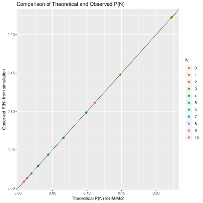
Figure 1: Comparison of theoretical equilibrium $\Prob(N)$ and observed proportions from simulation. Observation $N=1$ is obscured by $N=2$.

We see that the observed time average number of busy servers is 0.6661402 which is close to $0.\dot{6}$ the value for $\rho$. We can see that the observed mean waiting time is close to the expected mean waiting time. The expected number of customers in the system, from the distribution $\Prob(N)$ is close to the observed number of customers in the system. The entire distribution of $\Prob(N)$ is replicated in Figure 1.

7 Benchmark

7.1 Method

The compare the computational efficiency of each package we compute the departure times from a $M/M/2/\infty/n/FCFS$ queueing system, with $\lambda=1$ and $\mu=1.\dot{1}$. To understand how $n$ affects computation time we repeat the experiment 100 times for n = $10^{2},10^{3},10^{5}$ and $10^{6}$. We also repeat the experiment at $n=10^{7}$ for queuecomputer. We compare the median time taken for each combination of package and $n$.

The simulation was conducted on a system with Intel (R) Core(TM) i7-6700 CPU @ 3.40GHz running Debian GNU/Linux. The version of R is 3.5.1 “Feather spray" with simmer version 4.0.1 and queuecomputer version 0.8.3. The version of Python is 3.5.3 with simpy module version 3.0.11.

To assess the computation time for queuecomputer and simmer we use the microbenchmark function from the microbenchmark package (Rpkg_microbenchmark) with time = 100 and compute the median. Full details can be found in the supplementary material.

7.2 Results and discussion

The median computation time for each package and for varying numbers of customers from $100$ to $10^{6}$ customers (up to $10^{7}$ customers for queuecomputer) is shown in Figure 2. We observe phenomenal speedups for queuecomputer compared to both packages: compared to simpy speedups of 35 (at 100 customers) to 1000 (at $10^{6}$ customers) are observed, and for simmer speedups of 50 (at 100 customers) to 300 (at $10^{6}$ customers) are observed. The speedup is lower for smaller $n$ since queuecomputer approaches a minimum computation time.

Simulating 10 million customers takes less than 1 second for queuecomputer. We see no reason why queues of different arrival and service distributions should not have similar speedups. This is because, as mentioned earlier, any non-negative $\mathbf{(a,s)}$ could come from two exponential distributions.

Clearly, QDC and its implementation queuecomputer are a more computationally efficient way to simulate queueing systems of the form $G(t)/G(t)/K/\infty/M/FCFS$ than conventional DES algorithms implemented by simpy and simmer.

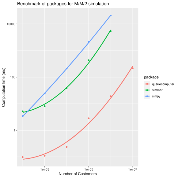
Figure 2: Computation time in milliseconds for varying numbers of passengers for each DES/queueing package. Each package returns exactly the same set of departure times since the same arrival and service times are supplied. The computation time reported here is the median time of 100 runs for each number of customers and each package. Intel (R) Core(TM) i7-6700 CPU @ 3.40GHz running Debian GNU/Linux.

8 Examples

8.1 Call center

We demonstrate queuecomputer by simulating a call center. The arrival time for each customer is the time that they called, and the service time is how long it takes for their problem to be resolved once they reach an available customer service representative. Let’s assume that the customers arrive by a homogeneous Poisson process over the course of the day.

R> library("queuecomputer") R> library("randomNames") R> library("ggplot2") R> set.seed(1) R> interarrivals <- rexp(20, 1) R> arrivals <- cumsum(interarrivals) R> customers <- randomNames(20, name.order = "first.last")

We also need a vector of service times for every customer.

R> service <- rexp(20, 0.5) R> head(service) [1] 2.6669670 1.2434810 0.4197332 0.6188957 2.2118725 1.5483755

We put the arrival and service times into the queue_step function to compute the departure times. Here we have set the number of customer service representatives to two. The “servers" argument is used for this input.

R> queue_obj <- queue_step(arrivals, service, servers = 2, + labels = customers) R> head(queue_obj$departures_{d}f)\Soutput#Atibble:6x7labelsarrivalsservicedepartureswaitingsystem_{t}imeserver<chr><dbl><dbl><dbl><dbl><dbl><int>1Johatam0.7552.673.420.2.6712Beatriz1.941.243.180.1.2423Devante2.080.4203.601.10e+01.5224Shaahira2.220.6194.041.20e+01.8215Ilea2.662.215.819.42e-13.1526Brianna5.551.557.102.22e-161.551\par WecanseethatJohatamarrivesfirstbutleavesafterBeatriz.Thisispossiblebecausetherearetwoservers.Johatam^{\prime}sservicetooksolongthatthenexttwocustomerswereservedbytheotherserver.It^{\prime}seasytoseehowthedeparturetimeswerecomputedinthissimpleexample.JohatamandBeatrizwerethefirstcustomersforeachserversowecancomputetheirdeparturetimebyjustaddingtheirservicetimestotheirarrivaltimes.\par\CodeChunk\Sinput R>firstcustomers<-arrivals[1:2]+service[1:2]R>firstcustomers\Soutput[1]3.4221493.180306\par Devante,however,hadtowaitforanavailableserver,sincehearrivedafterthefirsttwocustomersarrivedbutbeforethefirsttwocustomersdeparted.Hemustwaituntiloneofthesecustomersdepartsbeforehecanbeserved.Weaddthedeparturetimeofthefirstcustomerofserver2(Beatriz)tohisservicetimetocomputehisdeparturetime.\par\CodeChunk\Sinput R>firstcustomers[2]+service[3]\Soutput[1]3.600039\par Sothefirsttwocustomershadnowaitingtime,butDevantehadtowaitforanavailableserver.Wecancomputethewaitingtimesforallthreecustomersinthismanner:\par\CodeChunk\Sinput R>depart(queue_{o}bj)[1:3]-arrivals[1:3]-service[1:3]\Soutput[1]0.0000000.0000001.097774\par The\code{depart}functionisaconveniencefunctionforretrievingthedeparturetimesfroma\code{queue\_list}object.The\code{queue\_step}functionreturnsa\code{queue\_list}object.Thereisasummarymethodforthisobjectwithinthe\pkg{queuecomputer}package,thiscanbeaccessedbycalling\code{summary(departures)}.\par\CodeChunk\Sinput R>summary(queue_{o}bj)\Soutput Totalcustomers:20Missedcustomers:0Meanwaitingtime:1.15Meanresponsetime:3.69Utilizationfactor:0.834333359602573Meanqueuelength:0.858Meannumberofcustomersinsystem:2.42\par Theplotmethodin\pkg{queuecomputer}for\code{queue\_list}objectsusestheplottingpackage\pkg{ggplot2}\cite[citep]{(\@@bibref{AuthorsPhrase1Year}{Rpkg_ggplot2}{\@@citephrase{, }}{})}toreturnalistofplots.Weproducefourplots:ahistogramofthearrivalanddeparturetimes(Figure\ref{fig:histogram});aplotofthequeuelengthandnumberofcustomersinthesystemovertime(Figure\ref{fig:qlength});aplotofthewaitingandservicetimesforeachcustomer(Figure\ref{fig:customers});andaplotoftheempiricalcumulativedistributionfunctionforarrivalanddeparturetimes(Figure\ref{fig:ecdf}).Theseplotscorrespondtoselections$2,5$and$6$inthewhichargument,asimilarAPItotheplot.lmmethodinthestatspackage\text{<cite class="ltx\_cite ltx\_citemacro\_citep">(<span class="ltx\_ref ltx\_missing\_citation ltx\_ref\_self">Rproglang</span>)</cite>}.R>plot(queue{}_{o}bj,which=c(2,4,5,6)\text{Figure 3Figure 33Figure 33Histogramof}$