The energy-momentum tensor of electromagnetic fields in matter

Abstract

In this paper we present a complete resolution of the Abraham-Minkowski controversy about the energy-momentum tensor of the electromagnetic field in matter. This is done by introducing in our approach several new aspects which invalidate previous discussions. These are: 1)We show that for polarized matter the center of mass theorem is no longer valid in its usual form. A contribution related to microscopic spin should be considered. This allows to disregard the influencing argument done by Balacz in favor of Abraham’s momentum which discuss the motion of the center of mass of light interacting with a dielectric block. 2)The electromagnetic dipolar energy density $-\mathbf{P}\cdot\mathbf{E}$ contributes to the inertia of matter and should be incorporated covariantly to the the energy-momentum tensor of matter. This implies that there is also an electromagnetic component in matter’s momentum density given by $\mathbf{P}\times\mathbf{B}$ which accounts for the diference between Abraham and Minkowski’s momentum densities. The variation of this contribution explains the results of G. B. Walker, D. G. Lahoz and G. Walker’s experiment which until now was the only undisputed support to Abraham’s force. 3)A careful averaging of microscopic Lorentz’s force results in the unambiguos expression $f^{\mu}_{\mathrm{d}}=\frac{1}{2}D_{\alpha\beta}\partial^{\mu}F^{\alpha\beta}$ for the force density which the field exerts on matter. This force density is different to the ones used in most of the discussions and is consistent with all the experimental evidence. 4)Newton’s Third law or equivalently momentum conservation determines the electromagnetic energy-momentum tensor as the only one consistent with Maxwell’s equations whose divergence is minus the force density. It is $T_{\mathrm{S}}^{\mu\nu}-F^{\mu}_{\ \alpha}D^{\nu\alpha}$, where $T_{\mathrm{S}}$ is the standard tensor of the field in vacuum. This tensor is different from Abraham’s and Minkowski’s tensors, but one recovers Minkowski’s expression for the momentum density. In particular the energy density is different from Poynting’s expression but Poynting’s vector remains the same.. Our tensor is non-symmetric which allows the field to exert a distributed torque on matter. As a result of the specific form of the antisymmetric part of the constructed tensor, the spin density of the electromagnetic field decouples from the polarization of matter. To give further support to the proposed tensor, we also deduce its form using an alternative method based on direct averaging of the microscopic equations and on imposing consistency of the dipolar coupling. We use our results to discuss momentum and angular momentum exchange in various situations of physical interest. We find complete consistency of our equations in the description of the systems considered. We also show that several alternative expressions of the field energy-momentum tensor and force-density cannot be successfully used in all our examples. In particular we verify in two of these examples that the center of mass and spin introduced by us moves with constant velocity, but that the standard center of mass does not.

I Introduction

The definitions of the electromagnetic (EM) momentum in matter and of the energy-momentum density tensor of the electromagnetic field in matter has been discussed for over a century in what is known in the literature as the Abraham-Minkowski controversy. It is among the most prominent unsettled problems in classical physics. At the quantum level, resolution of the Abraham-Minkowski controversy is of paramount interest since it answers the fundamental question “what is the momentum of a photon in matter?” The main contenders in the dispute are the non-symmetric tensor constructed by Minkowski in 1908 Minkowski1908 and the symmetric one proposed by Abraham in 1909 Abraham1909 ; Abraham1910 , but other options have been discussed in the literature EinsteinL1908 ; EinsteinL1908b ; Beck1953 ; MarxG1956 ; deGrootS ; Peirls1976 ; Peirls1977 . Each construction provides a definite expression of the force exerted by the field on matter.

Although hundreds of papers investigate this issue many arguments lack precision in statement of the hypotheses and definitions or present an inadequate handling of their consequences. Various hypotheses and mechanisms that depart from the well-established Maxwell-Lorentz electromagnetic theory have been advanced. For example, proposed forms of the force density that the field exerts on matter are in general different from the force density imposed by the microscopic Lorentz force. Examples of this are the Minkowski force, the Abraham force and the Einstein-Laub force EinsteinL1908 . An even more puzzling hypothesis proposed in this context is the use of the theoretical quantity known as hidden momentum. Hidden momentum is the caloric of the XXth century. It was introduced by Shockley and James in SJ1967 as a resource to force the Center of Mass Motion Theorem (CMMT) Pryce1948 ; Hill1951 to hold, for systems which appear to have a contribution of electromagnetic momentum at rest. A weak version of the CMMT, states that the center of energy of an isolated system moves with a constant velocity in a chosen reference frame. A stronger version claims that such velocity is the total momentum of the system times $c^{2}$, divided by the energy. As we discuss below, these theorems have only limited validity. The true nature of the hidden momentum is never exhibited explicitly and the hypothesis implies very strange consequences on the mechanical behavior of physical systems when the value of the electromagnetic momentum changes.

An unsatisfactory situation exists because none of the sides have been able to convince the other of the validity of their arguments. This has led to an annoying posture well distributed in the literature TangM1961 ; Israel1977 ; Dewar1977 ; Kranys1979 ; Maugin1980 ; Pfeifer2007 ; Goto2011 which, relying on the fact that the energy-momentum tensor of the matter-field system may be split in many different forms, hypothesizes that all the alternatives are equivalent if adequately interpreted. In other words, it postulates that the problem cannot be settled theoretically and is not amenable to experimental elucidation.

The same unsatisfactory situation has induced some other people to think that both expressions may be used in the theoretical description with different meanings. Often, it is postulated that one of the expressions, usually Abraham’s, is the true mechanical momentum with the other being some other kind of momentum, either pseudo-momentum or quantum mechanical momentum Gordon1973 ; Nelson1991 ; Barnett2010 .

In this paper we show that fancy interpretations, exotic forces and hidden momentum are unnecessary hypotheses. We contend that the motivations to introduce them are wrong and that a totally consistent description of electromagnetic momentum exists within the framework of Maxwell-Lorentz electromagnetism. We show it is possible to give a definite answer to the question of which is the energy-momentum tensor of the electromagnetic field in matter; it is not necessary to take different expressions to represent the classical and quantum electromagnetic momentum in order to deal with the results of the experiments. The energy-momentum tensor for the electromagnetic field is neither Minkowski’s nor Abraham’s and we explain clearly why. We construct by two different methods an energy-momentum tensor of the electromagnetic field in matter that is consistent with the microscopic Lorentz force. Our construction finally resolves the long dated Abraham-Minkowski controversy and ratifies Minkowski’s expression for the momentum density. It is based on the observation that, in opposition to what is claimed in a large part of the recent literature, the matter and field contributions to the total energy-momentum tensor can be rigorously distinguished by focusing on the mechanical behavior of matter and using momentum conservation in the form of Newton’s Third Law.

To resolve this important debate, it is essential to describe very clearly the framework in which the discussion will be pursued. So we begin with a few remarks highlighting our suppositions and stating where we disagree with other authors.

Classical electromagnetism in material media is a very subtle subject with plenty of room for misunderstandings and confusion. To begin with, the same notation is often used for microscopic and macroscopic electromagnetic fields but they are very different objects. The microscopic field, at the classical level, allows for only monopolar couplings and interacts with all the microscopic charges and currents $\rho$ and ${\mathbf{j}}$. From the theoretical point of view, it is accepted that the description using the microscopic field should be valid up to the scale where quantum effects begin to be relevant. But in bulk matter this description cannot always be experimentally explored making it necessary to introduce the macroscopic field which is interpreted as an average field at some scale. The macroscopic field has a monopolar coupling with the free charges and currents $\rho_{\mathrm{f}}$ and ${\mathbf{j}_{\mathrm{f}}}$ and also has a dipolar coupling with the polarization vector ${\mathbf{P}}$ and the magnetization ${\mathbf{M}}$. Of course $\rho_{\mathrm{f}}$, ${\mathbf{j}_{\mathrm{f}}}$, ${\mathbf{P}}$ and ${\mathbf{M}}$ are manifestations of quantum and classical properties of the microscopic quantities $\rho$ and ${\mathbf{j}}$. The macroscopic fields may also have quadrupolar and higher order couplings although this possibility is usually not investigated. In agreement with the experimental evidence, we assume that Maxwell’s macroscopic equations are fulfilled. So, our first remark is that it is necessary to focus on the dipolar coupling of the macroscopic electromagnetic field to ${\mathbf{P}}$ and ${\mathbf{M}}$ instead of dwelling too much on the constitutive relations between ${\mathbf{E}}$ and ${\mathbf{B}}$ and ${\mathbf{D}}$ and ${\mathbf{H}}$. This approach is mandatory when dealing with ferromagnetic materials.

Our second remark concerns relativistic invariance. The understanding of the implications of relativistic invariance have evolved since the first decade of the past century when the controversy began. Putting things simply, a relativistic description requires one to work with covariant objects. Cavalier use of the electric and magnetic permeability constants $\epsilon$ and $\mu$ obscures the relativistic invariance of the equations. Attempts to regain relativistic invariance by introducing the velocity of the material media and switching between the laboratory frame and the co-moving frame of matter without choosing convenient covariant objects is a limiting procedure. Such attempts introduce the well known inconsistency of the concept of rigid body and relativity. To guarantee the covariance of Maxwell’s equations in a material medium, it is sufficient and necessary that the fields ${\mathbf{P}}$ and ${\mathbf{M}}$ and, as a consequence, ${\mathbf{D}}$ and ${\mathbf{H}}$ transform in the same way as the electromagnetic fields ${\mathbf{E}}$ and ${\mathbf{B}}$.

Our third point concerns the force density that the field exerts on matter. The force density and the total force are observable quantities which can be measured in a manifold of situations by observing the mechanical behavior of matter. The energy-momentum tensor of matter is determined as the tensor whose four-divergence is the force density. It includes all the energy parcels which contribute to inertia, even those of electromagnetic origin. Momentum conservation, a consequence of the homogeneity of space, then determines the energy-momentum tensor of the field as the tensor whose four-divergence is the negative of the force density. The force density is also subjected to theoretical constraints. It should be relativistically covariant and should reduce to the Lorentz force when a microscopic description of the electric and magnetic dipoles is re-introduced. Einstein-Laub’s, Minkowski’s, Abraham’s and the Lorentz-Ampere force densities do not satisfy these criteria. The force density $f^{\mu}_{\mathrm{d}}=\frac{1}{2}D_{\alpha\beta}\partial^{\mu}F^{\alpha\beta}$ does, as discussed below.

Our fourth introductory remark addresses the asymmetry of the energy-momentum tensor. It is frequently assumed that the energy-momentum tensor of an isolated system should be symmetric for one of the following three reasons. 1) To guarantee the conservation of angular momentum. 2) Because there is a theorem BelF1939 ; Rosenfeld1940 ; Pauli1941 ; CvV1968 which states that it is always possible to symmetrize the tensor. 3) Because it is imposed by Einstein’s equations of gravitation. None of these reasons is valid. The energy-momentum tensor should be symmetric for conserving the orbital angular momentum, not the total angular momentum. There is no symmetrizing theorem for the energy-momentum tensor. Belinfante-Rosenfeld’s construction BelF1939 ; Rosenfeld1940 yields a symmetric tensor, made up from the energy-momentum tensor and derivatives of the spin density, which is not the mechanical energy-momentum tensor. Einstein’s equations impose that their source, not the mechanical energy-momentum tensor, should be symmetric. The source of Einstein’s equations is physically a different object and there is no contradiction in relating it to the Belinfante-Rosenfeld tensor.

Our next observation is related to the hidden momentum approach and the CMMT. In its usual form the CMMT is not valid in relativistic mechanics. The CMMT was invoked repeatedly in discussions of the electromagnetic momentum to justify introduction of hidden momentum. It also was used by Balazs to support Abraham’s momentum arguing on a mechanical example. But the CMMT is not valid for systems with spin in general and is not valid for the electromagnetic field interacting with polarizable matter in particular. What is valid for systems which include spin and for which total angular momentum is conserved, is a modified version of the theorem which states that for an isolated system a quantity which we call the center of mass and spin behaves inertially. This fact has been overlooked in all previous discussions.

Our final point is about the distinction between the electromagnetic field and the electromagnetic wave when such a wave is propagating through a medium. In that case, traveling together with the electromagnetic fields there are disturbances of ${\mathbf{P}}$, ${\mathbf{M}}$ and the internal stress. The energy and momentum contributions of these disturbances should appear in the energy-momentum-stress tensor of matter. Poynting’s equation which is a consequence of Maxwell’s equations for homogeneous media is best suited to describe the wave as a whole. In particular Poynting’s energy density, as we will argue in this article, is the energy of the wave, not the energy of just the field. Many of the misunderstandings concerning the energy-momentum tensor of the field may be traced back to this observation. This point is also very important to understand the meaning of the von Laue-Møller vLaue1950 ; Moller condition on the velocity of propagation of the energy density.

Our paper is organized as follows. In section II, we show the limitations of CMMT for systems with spin, discuss the concept of center of mass and spin, and deduce the modified version of the theorem which holds for those systems. In section III, we discuss Poynting’s equation and its generalizations. In section IV, a brief discussion of the Abraham-Minkowski controversy is presented. The von Laue-Møller criterion and the Balazs argument are considered. In section V, we obtain an expression of the force which is covariant and reduces to the Lorentz force in the microscopic description. Using this force in section VI, we construct the true energy-momentum tensor of the field. Although the energy density is not given by Poynting’ s expression one recovers Minkowski’s expression for the momentum density. This confirms our recent computation MedinaandS2017 where in a simple setup we show that if Maxwell’s equations and Ohm’s law are valid, only Minkowski’s momentum density is consistent with momentum conservation. On the other hand, we recognize Poynting’s energy density and Minkowski’s tensor as the objects which describe the whole electromagnetic wave thus satisfying the von Laue-Møller criterion. In section VII, we take an alternate path and re-obtain our results by directly averaging the microscopic field equations and imposing consistency with the results of a macroscopic field with an arbitrary dipolar coupling. In the remaining sections we discuss some examples and consequences. In section VIII, we compare the experimental consequences that predict the force density we proposed with the other alternatives. We propose a method to elucidate which is the true force density by measuring electro and magnetostriction. In section IX we consider the transmission of an electromagnetic wave in a medium, which corresponds to the setup of Balazs. We compute the force exerted by the fields on matter and show that the standard CMMT does not hold, but that instead the center of mass and spin behaves inertially, as we claim it should. In section X, we consider an interesting magnet-charge system and show that its description is fully consistent with our equations. We also show that, for this system, the center of mass and spin behave inertially in a non trivial way. In section XI, we consider a situation in which there is exchange of angular momentum between matter and field, which can be handled neatly within our approach. Section XII contains our conclusions.

II Angular momentum and the CM motion theorem

II.1 Orbital and spin angular momentum

Let us consider a system with an energy-momentum tensor $T^{\mu\nu}$ upon which a force density $f^{\mu}$ is exerted. A local version of Newton’s Second Law holds

$$\partial_{\nu}T^{\mu\nu}=f^{\mu}\ .$$ (1)

For a localized system with $f^{\mu}=0$ the total energy $U=\int T^{00}dV$ and the total momentum $p^{i}=c^{-1}\int T^{i0}dV$ are conserved. The current density of the orbital angular momentum is defined as $L^{\mu\nu\alpha}=x^{\mu}T^{\nu\alpha}-x^{\nu}T^{\mu\alpha}$ and it satisfies identically

$$\partial_{\alpha}L^{\mu\nu\alpha}=T^{\nu\mu}-T^{\mu\nu}+x^{\mu}f^{\nu}-x^{\nu}f^{\mu}\ .$$ (2)

The last two terms of the right hand side of this equation represent the torque of the force density. The asymmetry of the energy-momentum tensor plays the role of a torque density exerted on the orbital angular momentum. If the force density is zero and there are neither a torque density $\tau^{\mu\nu}$ nor a spin density $S^{\mu\nu\alpha}$, the orbital angular momentum is conserved and the energy-momentum tensor must be symmetric. This is not necessarily true when these conditions are not fulfilled Papapetrou1949 . In presence of spin the relevant quantity is the total angular momentum $J^{\mu\nu\alpha}=L^{\mu\nu\alpha}+S^{\mu\nu\alpha}$ whose equation of motion

$$\partial_{\alpha}J^{\mu\nu\alpha}=\tau^{\mu\nu}+x^{\mu}f^{\nu}-x^{\nu}f^{\mu}\ ,$$ (3)

allows for an external torque density $\tau^{\mu\nu}$. Then the right hand side is the total torque density acting on the system. For isolated systems one assumes that the total angular momentum is conserved.

Combining (2) and (3) the spin equation is obtained

$$\partial_{\alpha}S^{\mu\nu\alpha}=T^{\mu\nu}-T^{\nu\mu}+\tau^{\mu\nu}\ .$$ (4)

The internal torque density represented by the asymmetry of $T^{\mu\nu}$ couples spin and orbital angular momenta. If the system has no spin, but there is a distributed torque then $T^{\mu\nu}-T^{\nu\mu}=-\tau^{\mu\nu}$. Another interesting case is when the system is isolated; the total angular momentum is conserved, but there may be an exchange between spin and orbital angular momentum as a result of microscopic interactions. That is what happens in a magnet when the magnetization changes. Since the magnetization is proportional to the spatial part of the spin density, if a demagnetization occurs, spin becomes orbital angular momentum. This is the Einstein-de Haas Einstein-deHaas1915 effect which is used routinely to measure the gyromagnetic ratio BarKen1952 of atoms and molecules and provides an example where the total energy-momentum tensor cannot be symmetric. The statement, found some times in the literature Abraham1910 , that conservation of angular momentum requires a symmetric energy-momentum tensor, is not only false but in this and other cases the opposite is true: conservation of (total) angular momentum requires that the total energy-momentum tensor should be non-symmetric.

II.2 The boost momentum

The temporal component of the angular momentum equation plays an important role in the treatment of the CMMT. The total angular momentum of a system $J^{\mu\nu}=c^{-1}\int J^{\mu\nu 0}\,dV$ is an antisymmetric tensor. The spatial part of this tensor is the angular momentum axial vector $\mathbf{J}$, $J^{ij}=\epsilon_{ijk}J^{k}$. The temporal components $J^{0k}$ transform as a polar vector, which is a different physical quantity, in the same sense that $\mathbf{E}$ is different from $\mathbf{B}$. This quantity is seldom treated in the literature and its physical meaning is not well appreciated. There is not even a generally accepted name for it. A sensible name could be the boost momentum, since $\{J^{0k}\}$ are the generators of the Lorentz boosts, or the arrow of angular momentum as we proposed elsewhere MedandSf . To better understand the significance of the boost momentum consider a non-relativistic particle of mass $m$, position $\mathbf{x}$ and momentum $\mathbf{p}$. In a different frame of reference moving with velocity $c\bm{\beta}$ the position is incremented by $\Delta\mathbf{x}=-ct\bm{\beta}$, and the momentum is incremented by $\Delta\mathbf{p}=-mc\bm{\beta}$. The quantity which has the proper Poisson brackets to generate this transformation is $\bm{\beta}\cdot\mathbf{g}$ with $\mathbf{g}=ct\mathbf{p}-mc\mathbf{x}$. For a system of particles of center of mass $\mathbf{X}$, total mass $M$ and total momentum $\mathbf{P}$ the generator of the Galilean boost is $\mathbf{g}=ct\mathbf{P}-Mc\mathbf{X}$. Conservation of this quantity is equivalent to the CMMT. Note that $\mathbf{g}$ corresponds to the orbital boost momentum $L^{0k}$ of the relativistic case. On the other hand, the Galilean boost does not modify the angular velocitiy or the shape of a body, that is, it does not modify the spin of the system (the angular momentum with respect to the CM). In Newtonian physics the spin commutes with the Galilean boost, and therefore the existence of spin does not impair the CMMT. This means that spin boost momentum does not have a non-relativistic counterpart.

Like boost momentum the temporal components of the torque also form a polar vector which is different from the spatial torque. In some particular reference frame a system may in principle have a non-zero boost momentum and a vanishing $\mathbf{J}$. This is also true for the torque.

II.3 The CM motion theorem

Let us consider an isolated, localized system with a non-symmetric energy-momentum tensor upon which no forces are exerted so that, $\partial_{\nu}T^{\mu\nu}=0$.

To discuss the CMMT define the center of mass by

$$X^{i}_{T}=\frac{1}{U}\int x^{i}T^{00}\,dV\ .$$ (5)

Here the index $T$ refers to the fact that the CM depends on $T^{\mu\nu}$. It is worth remarking that this definition of center of mass depends on the frame of reference. If in some frame of reference at time $t$ the center of mass is $\mathbf{X}$, and the event $(t,\mathbf{X})$ is labeled by $(t^{\prime},\mathbf{X}^{\prime})$ in some other frame, and if $\mathbf{Y}^{\prime}$ is the CM in the new frame at time $t^{\prime}$, then in general $\mathbf{Y}^{\prime}\not=\mathbf{X}^{\prime}$. Statements about centers of mass should be done with caution. For example, the fact that the CM moves with constant velocity in some frame of reference does not imply that the CM also moves with constant velocity in some other frame of reference.

If there is no spin, $T^{\mu\nu}$ is symmetric and orbital angular momentum $L^{\mu\nu}=c^{-1}\int L^{\mu\nu 0}\,dV$ is conserved. Then, it is easy to see that the center of mass moves with velocity $c^{2}p^{i}/U$. Instead, for non-symmetric $T^{\mu\nu}$ it is also easy to see that

$$\dot{X}^{i}_{T}=\frac{c}{U}\int T^{0i}\,dV\ .$$ (6)

Note that what appears in (6) is the energy current density, not the momentum density. The non-vanishing temporal spin of the system jeopardizes the validity of the CMMT. To see this define the spin matrix $S^{\mu\nu}=c^{-1}\int S^{\mu\nu 0}\,dV$ and consider the quantity

$$X^{i}_{S}=-\frac{c}{U}S^{0i}\ .$$ (7)

From the conservation of total angular momentum it follows that

$$\frac{d}{dt}X^{i}_{S} = \frac{c}{U}\frac{d}{dt}L^{0i}=\frac{1}{U}\frac{d}{dt}\int\big{[}x^{0}T^{i0}-x^{i}T^{00}\big{]}dV$$ (8)

$$= \frac{c^{2}p^{i}}{U}-\frac{d}{dt}X^{i}_{T}\ .$$

This shows that the center of mass and spin defined by

$$X^{i}_{\Theta}=X^{i}_{T}+X^{i}_{S}$$ (9)

moves with constant velocity $\dot{X}^{i}_{\Theta}=c^{2}p^{i}/U$.

It is worth noting MedandSe that $X^{i}_{\Theta}$ corresponds to the center of mass computed using the symmetric Belinfante-Rosenfeld’s tensor $\Theta^{\mu\nu}$, which is a combination of the energy-momentum tensor and the spin density. In the literature Belinfante-Rosenfeld’s tensor is frequently considered as an improved symmetrized energy-momentum tensor but we consider that this interpretation is wrong, at least from the mechanical point of view.

As a simple illustration of the ideas presented in this section, consider an isolated uniformly magnetized sphere with a device included which heats the sphere respecting the symmetry. In the rest frame the spin, which is proportional to the magnetization, is purely spatial and both the center of mass and the center of mass and spin are located at the center of the sphere. As the sphere heats the magnetization diminishes and finally vanishes and by conservation of total angular momentum the sphere rotates. The center of mass and the center of mass and spin remain in place. Looking at this system from a reference frame where the sphere is moving in a direction which is perpendicular to magnetization, the center of mass is initially at the center of the sphere. The temporal components of spin do not vanish and the center of mass and spin is displaced from the center of the sphere in the direction perpendicular to the magnetization and to the velocity. When the magnetization disappears the sphere is rotating about the axis which is in the former direction of the magnetization. The velocity of matter in one side of the sphere is greater than the velocity in the other side, and the center of mass is now displaced with respect to the geometric center. Clearly, it has been accelerated. It may be shown MedandSf that the center of mass and spin (9) which in the final situation coincides with the center of mass behaves inertially along the whole process.

III Poynting’s energy density and energy flux

III.1 The dipolar density tensor

In Gauss units and using the metric tensor $\eta^{\mu\nu}=\mathrm{diag}(-1,1,1,1)$, the electromagnetic field tensor (either microscopic or macroscopic) is $F_{\alpha\beta}=\partial_{\alpha}A_{\beta}-\partial_{\beta}A_{\alpha}$, and is related to the electric and magnetic fields by $F^{0i}=-F^{i0}=E_{i}$ and $F^{ij}=\epsilon_{ijk}B_{k}$.

The traditional way of treating polarizable matter is to assume that there are microscopic electric and magnetic dipoles. The polarization $\mathbf{P}$ and magnetization $\mathbf{M}$ are defined so that an element of material of volume $dV$ has a total electric dipole moment $\mathbf{P}dV$ due to the electric dipoles and a total magnetic moment $\mathbf{M}dV$ due to the magnetic dipoles. In the non-relativistic approximation this picture works fine but it is problematic in the general case, since moving electric and magnetic dipoles have moments of both kinds. Because of this reason in this paper we refrain from using those microscopic entities. In the following we present a phenomenological and macroscopic definition of $\mathbf{P}$ and $\mathbf{M}$.

The fields and currents used in macroscopic physics are averages of the microscopic fields and currents over small space-time regions. As usual we will assume, that at a microscopic scale the equations for the vacuum hold. In a material sample at a macroscopic scale, in addition to the averaged current density of free charges $j_{\mathrm{f}}^{\mu}=(c\rho_{\mathrm{f}},{\mathbf{j}}_{\mathrm{f}})$, there are electric and magnetic dipole moments that couple directly to the EM tensor $F^{\mu\nu}$. These dipole moments are due to bound charges. The total bound charge in any piece of material is always zero. This is a kind of mechanical constraint. The fields produced by the dipoles are described by the current density four-vector of bound charges $j^{\mu}_{\mathrm{b}}$. Any piece of material may have a bound charge in the surface $Q_{\mathrm{bS}}$ and a bound charge in the bulk $Q_{\mathrm{bV}}$, but the total bound charge should always be zero, $Q_{\mathrm{bS}}+Q_{\mathrm{bV}}=0$. This behavior is described in terms of $\mathbf{P}$, defined inside the material, if the charge density of bound charges is $\rho_{\mathrm{b}}=-\nabla\cdot\mathbf{P}$ and the surface charge density is $\sigma_{\mathbf{b}}=\mathbf{P}\cdot\hat{\mathbf{n}}$, where $\hat{\mathbf{n}}$ is the normal unitary vector of the surface. The continuity equation for the bound charges is

$$0=\frac{\partial\rho_{\mathrm{b}}}{\partial t}+\nabla\cdot\mathbf{j}_{\mathrm{b}}=\nabla\cdot(\mathbf{j}_{\mathrm{b}}-\dot{\mathbf{P}})\ .$$ (10)

In general, in addition to the polarization current density $\dot{\mathbf{P}}$, a divergence-less magnetic current density $\mathbf{j}_{\mathrm{m}}=\mathbf{j}_{\mathrm{b}}-\dot{\mathbf{P}}$ also contributes to the bound current density. This magnetic current density is not related to any macroscopic motion of charge, and is expressed as the rotational of the magnetization field $\mathbf{j}_{\mathrm{m}}=c\nabla\times\mathbf{M}$. $\mathbf{M}$ vanishes outside the material. Since there is no total magnetic current crossing a piece of material, in the surface of any piece of material there is also a magnetic surface current density $\mathbf{\Sigma}_{\mathrm{m}}=c\mathbf{M}\times\hat{\mathbf{n}}$.

An element of material of volume $dV$ has an electrical dipole moment $d\mathbf{d}=\mathbf{P}dV$ and a magnetic dipole moment $d\mathbf{m}=\mathbf{M}dV$ due to the surface charges and surface currents respectively. The bulk contributions which go like $r^{3}$ are negligible with respect to the surface ones that go like $r^{2}$.

For a covariant description one should define the space-time dipolar density $D_{\alpha\beta}$, whose spatial part is the magnetization density $D_{ij}=\epsilon_{ijk}M_{k}$ and whose temporal part is the polarization $D_{0k}=-D_{k0}=P_{k}$. The bound current density is then

$$j^{\mu}_{\mathrm{b}}=c\partial_{\nu}D^{\mu\nu}\ .$$ (11)

As mentioned before, in order to have relativistic invariance, $D_{\alpha\beta}$ should be a Lorentz tensor. The fact that $D_{\alpha\beta}$ is antisymmetric implies the conservation of the bound current $\partial_{\mu}j^{\mu}_{\mathrm{b}}=c\partial_{\mu}\partial_{\nu}D^{\mu\nu}=0$.

III.2 Maxwell’s equations

The displacement vector and the magnetizing field vector are given in our notation by $\mathbf{D}=\mathbf{E}+4\pi\mathbf{P}$ and $\mathbf{H}=\mathbf{B}-4\pi\mathbf{M}$. In what follows we assume that Maxwell’s macroscopic equations

$$\nabla\cdot{\mathbf{D}} = 4\pi\rho_{\mathrm{f}}\ ,\qquad\nabla\times{\mathbf{E}}+\frac{1}{c}\frac{\partial{\mathbf{B}}}{\partial t}=0\ ,$$

$$\nabla\cdot{\mathbf{B}} = 0\ ,\qquad\nabla\times{\mathbf{H}}-\frac{1}{c}\frac{\partial{\mathbf{D}}}{\partial t}=\frac{4\pi}{c}{\mathbf{j}}_{\mathrm{f}}$$ (12)

are valid in any reference frame. To cast this in covariant notation one defines

$$H^{\mu\nu}=F^{\mu\nu}-4\pi D^{\mu\nu}$$ (13)

whose components are related to the magnetizing field $\mathbf{H}$ and to the electric displacement $\mathbf{D}$ by $H^{ij}=\epsilon_{ijk}H_{k}$ and $H^{0i}=D_{i}$.

The field equations become

$$\partial_{\beta}H^{\alpha\beta}=\frac{4\pi}{c}j_{\mathrm{f}}^{\alpha}\ ,$$ (14)

$$\partial_{\mu}F_{\nu\lambda}+\partial_{\nu}F_{\lambda\mu}+\partial_{\lambda}F_{\mu\nu}=0\ .$$ (15)

The second of these equations is the Bianchi’s identity. The first equation written in terms of the macroscopic electromagnetic field is

$$\partial_{\nu}F^{\mu\nu}=\frac{4\pi}{c}(j_{\mathrm{f}}^{\mu}+j_{\mathrm{b}}^{\mu})\ .$$ (16)

III.3 The susceptibility and permeability tensors

Isotropic linear materials are characterized by the familiar relations $\mathbf{D}=\epsilon\mathbf{E}$ and $\mathbf{H}=1/\mu\mathbf{B}$. These relations are meant to be valid in a particular reference frame, which for homogeneous, isotropic media is the rest frame of matter. But much more complicated situations may be contemplated, and in order to obtain a relativistic invariant description it is necessary to introduce generalized relations in terms of a four indexes susceptibility tensor. They take the form,

$$D_{\alpha\beta}=\frac{1}{2}\chi_{\alpha\beta\gamma\delta}F^{\gamma\delta}\ .$$ (17)

The susceptibilities form a four-tensor of four indexes with the following symmetries

$$\chi_{\alpha\beta\gamma\delta}=\chi_{\gamma\delta\alpha\beta}=-\chi_{\beta\alpha\gamma\delta}\ .$$ (18)

The four-tensor $\chi_{\alpha\beta\gamma\delta}$ includes the susceptibilities three-tensors, the electric-electric $\chi^{\mathrm{(e-e)}}$, the magnetic-magnetic $\chi^{\mathrm{(m-m)}}$, the electric-magnetic $\chi^{\mathrm{(e-m)}}$ and the magnetic-electric $\chi^{\mathrm{(m-e)}}$. The first two are symmetric tensors, and of the last two one is the transpose of the other. In total there are $21$ independent components. The three-tensors are defined by

$$P_{i}=\chi^{\mathrm{(e-e)}}_{ij}E_{j}+\chi^{\mathrm{(e-m)}}_{ij}B_{j}$$ (19)

and

$$M_{i}=\chi^{\mathrm{(m-m)}}_{ij}B_{j}+\chi^{\mathrm{(m-e)}}_{ij}E_{j}\ .$$ (20)

Note that $\chi^{\mathrm{(m-m)}}$ is different from the traditional magnetic susceptibility tensor $\tilde{\chi}$, which is defined using $\mathbf{H}$ instead of $\mathbf{B}$, $\chi^{\mathrm{(m-m)}}=\tilde{\chi}(I+4\pi\tilde{\chi})^{-1}$.

The relationship between the four-tensor and the three-tensors is

$$\chi^{\mathrm{(e-e)}}_{ij} = \chi_{0i0j}\ ,$$ (21)

$$\chi^{\mathrm{(m-m)}}_{ij} = \frac{1}{4}\epsilon_{ilm}\epsilon_{jfg}\chi_{lmfg}\ ,$$ (22)

$$\chi^{\mathrm{(e-m)}}_{ij} = \frac{1}{2}\epsilon_{jfg}\chi_{0ifg}\ ,$$ (23)

$$\chi^{\mathrm{(m-e)}}_{ij} = \frac{1}{2}\epsilon_{ifg}\chi_{fg0j}\ .$$ (24)

The proper way of treating the transformation of the susceptibilities when the frame of reference is changed is by transforming the four-tensor. When matter is at rest and the material is centrosymmetric the mixed pseudo-tensors vanish, $\chi^{\mathrm{(e-m)}}=\chi^{\mathrm{(m-e)}}=0$. This property is lost in other frames of reference.

Equivalent relations may be written in terms of the permeability tensor. Using (13) one has

$$H_{\alpha\beta}=\frac{1}{2}\mu_{\alpha\beta\gamma\delta}F^{\gamma\delta}\ .$$ (25)

with

$$\mu_{\alpha\beta\gamma\delta}=\delta_{\alpha\gamma}\delta_{\beta\delta}-\delta_{\alpha\delta}\delta_{\beta\gamma}+4\pi\chi_{\alpha\beta\gamma\delta}$$ (26)

The permeability tensor has the same symmetry properties as the susceptibility tensor. In particular one has,

$$D_{i}=\epsilon_{ij}E_{j}+\xi_{ij}B_{j}$$ (27)

and

$$H_{i}=\zeta_{ij}B_{j}+\eta_{ij}E_{j}\ .$$ (28)

The tensors $\epsilon_{ij}$ and $\zeta_{ij}$ must be symmetric and the pseudo-tensors $\xi_{ij}$ and $\eta_{ij}$ are related by $\eta_{ij}=-\xi_{ji}$. These conditions are preserved by Lorentz transformations. At rest, for a centrosymmetric material, the pseudo-tensors vanish, but that is not true in the general case.

In the particular case of a homogeneous isotropic material with a dielectric constant $\epsilon$ and magnetic permeability $\mu$, which in the rest frame satisfy $\mathbf{D}^{\prime}=\epsilon\mathbf{E}^{\prime}$ and $\mathbf{B}^{\prime}=\mu\mathbf{H}^{\prime}$ one may obtain the permeability tensor by expressing the fields in the rest frame in terms of those in the moving frame. The familiar relations for the transformed fields are,

$$\mathbf{D}+\bm{\beta}\times\mathbf{H}=\epsilon(\mathbf{E}+\bm{\beta}\times\mathbf{B})$$ (29)

and

$$\mathbf{H}-\bm{\beta}\times\mathbf{D}=\frac{1}{\mu}(\mathbf{B}-\bm{\beta}\times\mathbf{E})\ ,$$ (30)

where $c\bm{\beta}$ is the velocity of the medium.

Solving these equations we get, $\gamma=1/\sqrt{1-\beta^{2}}$,

$$\epsilon_{jk}=\gamma^{2}[(\epsilon-\beta^{2}/\mu)\delta_{jk}-(\epsilon-1/\mu)\beta_{j}\beta_{k}]\ ,$$ (31)

$$\zeta_{jk}=\gamma^{2}[(1/\mu-\epsilon\beta^{2})\delta_{jk}-(\epsilon-1/\mu)\beta_{j}\beta_{k}]\ ,$$ (32)

and

$$\xi_{jk}=-\eta_{jk}=\gamma^{2}(\epsilon-1/\mu)\epsilon_{jlk}\beta_{l}\ .$$ (33)

III.4 Energy flux equation and Poynting’s equation

The flux of energy is determined by the following relation which is a direct consequence of macroscopic Maxwell’s equations (III.2)

$$\frac{1}{4\pi}\Big{(}\mathbf{E}\cdot\frac{\partial\mathbf{D}}{\partial t} + \mathbf{H}\cdot\frac{\partial\mathbf{B}}{\partial t}\Big{)}$$ (34)

$$= -\frac{c}{4\pi}\nabla\cdot({\mathbf{E}}\times{\mathbf{H}})-{\mathbf{E}}\cdot{\mathbf{j}}_{\mathrm{f}}\ .$$

This may be written in the two alternative forms

$$\frac{1}{8\pi}\frac{\partial}{\partial t}(B^{2} + E^{2})+\frac{\partial}{\partial t}({\mathbf{E}}\cdot{\mathbf{P}})+\frac{c}{4\pi}\nabla\cdot({\mathbf{E}}\times{\mathbf{H}})$$ (35)

$$= -{\mathbf{E}}\cdot{\mathbf{j}}_{\mathrm{f}}+{\mathbf{P}}\cdot\frac{\partial{\mathbf{E}}}{\partial t}+{\mathbf{M}}\cdot\frac{\partial{\mathbf{B}}}{\partial t}$$

and

$$\frac{1}{8\pi}\frac{\partial}{\partial t}(B^{2} + E^{2})+\frac{c}{4\pi}\nabla\cdot({\mathbf{E}}\times{\mathbf{B}})$$ (36)

$$= -{\mathbf{E}}\cdot({\mathbf{j}}_{\mathrm{f}}+{\mathbf{j}}_{\mathrm{b}})\ .$$

The different terms in these equations should describe the energy density and the energy current density of the field and the power supplied to matter by the field. There is clearly more that one way to establish these correspondences, but we will argue below that there is one way that should be preferred.

In 1884 Poynting Poynting proposed his energy conservation equation using the particular case of these equations that applies for homogeneous isotropic materials with time-independent linear susceptibilities $\mathbf{D}=\epsilon\mathbf{E}$ and $\mathbf{H}=1/\mu\mathbf{B}$. He postulates that the energy density is

$$u_{\mathrm{P}}=\frac{1}{8\pi}(\mathbf{E}\cdot\mathbf{D}+\mathbf{H}\cdot\mathbf{B})\ .$$ (37)

With the mentioned restrictions on the medium it follows that

$$\frac{\partial u_{\mathrm{P}}}{\partial t}=\frac{1}{4\pi}\Big{(}\mathbf{E}\cdot\frac{\partial\mathbf{D}}{\partial t}+\mathbf{H}\cdot\frac{\partial\mathbf{B}}{\partial t}\Big{)}$$ (38)

and equation (34) reduces to

$$\frac{\partial u_{\mathrm{P}}}{\partial t}+\nabla\cdot\mathbf{S}=-\mathbf{E}\cdot\mathbf{j}_{\mathrm{f}}\ ,$$ (39)

where the energy current density $\mathbf{S}$ is Poynting’s vector,

$$\mathbf{S}=\frac{c}{4\pi}\mathbf{E}\times\mathbf{H}\ .$$ (40)

This led to the interpretation of $\mathbf{S}$ as the energy current density of the electromagnetic disturbance, and $\mathbf{E}\cdot\mathbf{j}_{\mathrm{f}}$ as the time rate of work done by the field on the free charges. No work is done on the polarizable matter. At this point there is place to ask if $u_{\mathrm{P}}$ should necessarily be interpreted as the energy density of the field and if the work done on the free charges is all the work done by the field on matter. In the following sections we argue that the answers to these questions are both negative.

The condition (38) is valid also for anisotropic linear susceptibilities. Poynting’s energy density for an anisotropic material in any reference frame is given by

$$u_{\mathrm{P}}=\frac{1}{8\pi}(\epsilon_{jk}E_{j}E_{k}+\zeta_{jk}B_{j}B_{k})\ .$$ (41)

From this expression it is readily shown that for time-independent tensors the relationship (38) is fulfilled, and that therefore Poynting’s equation (39) is valid.

Note that in order for $\epsilon_{jk}$ and $\zeta_{jk}$ be time independent in any reference frame, it is required that the medium properties are not only time-independent but also homogeneous. Poynting’s equation is valid in any frame of reference only for material media which are homogeneous, time-independent, and that are moving in a uniform translation.

III.5 Electrostatic energy

The essential differences between non-dipolar and dipolar matter already appear in electrostatics. In this subsection we discuss the physical significance of various ways of defining electrostatic energy for dipolar matter. Let us start by considering non-dipolar matter. The energy of a system of charges is the sum of electrostatic interaction energy $U_{\mathrm{e}}$ and $U_{\mathrm{M}}$ which represents all other kinds of energies. The electrostatic energy is

$$U_{\mathrm{e}}=\frac{1}{2}\int\rho\phi\,dV\ ,$$ (42)

which can also be expressed as

$$U_{\mathrm{e}}=\frac{1}{8\pi}\int E^{2}\,dV\ .$$ (43)

If it is assumed that the matter energy is distributed in the volume there would be a matter energy density $u_{\mathrm{M}}$ to be added to the standard field energy density $u_{\mathrm{S}}$ which represents the electrostatic interaction

$$u_{\mathrm{S}}=\frac{1}{8\pi}E^{2}\ .$$ (44)

For dipolar matter where there is a polarization $\mathbf{P}$ two facts have to be considered. 1) The energy density of matter becomes polarization-dependent and should be now denoted by $u_{\mathrm{b}}(\mathbf{P})$ (here the label b stands for bare). 2) $u_{\mathrm{S}}$ still represents the total electrostatic energy, but a part of this energy density, given by

$$u_{\mathrm{d}}=-\mathbf{P}\cdot\mathbf{E}$$ (45)

corresponds to the interaction energy of electric dipole moments. The total energy density is given by $u_{\mathrm{b}}(\mathbf{P})+u_{\mathrm{S}}$, but $u_{\mathrm{d}}$ should be considered part of the energy of matter, since it is attached to it and contributes to its inertia. The energy density of (dressed) matter is then

$$u_{\mathrm{M}}=u_{\mathrm{b}}(\mathbf{P})+u_{\mathrm{d}}\ .$$ (46)

Correspondingly, the dipolar interaction energy must be subtracted from the standard field energy density in order to obtain the actual field energy density

$$u=u_{\mathrm{S}}-u_{\mathrm{d}}\ .$$ (47)

This modifies the expression of power released to matter. The power density on the bare dipoles is $\mathbf{E}\cdot\dot{\mathbf{P}}$, whereas for the dressed dipoles it is $-\mathbf{P}\cdot\dot{\mathbf{E}}$. In section VI, we show that the generalization of (47), which includes the magnetic field contribution should be regarded as the energy density of the field.

This field energy density is not only different from the standard one for non-dipolar matter, it also differs from the Poynting density for dipolar matter $\mathbf{E}\cdot\mathbf{D}/8\pi$. To compare with this last density consider an isotropic medium with linear polarizability. The bare matter density $u_{\mathrm{b}}$ should have a deformation term quadratic in $\mathbf{P}$

$$u_{\mathrm{b}}(\mathbf{P})=u_{\mathrm{b}}(0)+\frac{1}{2\chi}P^{2}\ .$$ (48)

Here $\chi$ is the electric susceptibility. When an electric field is present the matter polarizes itself by minimizing $u_{\mathrm{M}}$ with the result $\mathbf{P}=\chi\mathbf{E}$. The dressed matter changes its energy by an amount of $-\mathbf{P}\cdot\mathbf{E}/2$ which is the sum of the electrostatic energy $-\mathbf{P}\cdot\mathbf{E}$ and the deformation energy $\mathbf{P}\cdot\mathbf{E}/2$. The bare matter increases its energy by the deformation energy. Poynting’s density adds the deformation energy to the standard energy density $u_{\mathrm{S}}$ of the field. This density is useful for determining the total energy of a system (field plus matter), for example in a capacitor, but it cannot be used for determining the energy exchange between matter and field. Poynting density is useless for matter with non-linear polarizabilities.

IV Abraham-Minkowski controversy

IV.1 Splitting the Electromagnetic tensor

To discuss electromagnetic momentum it is necessary to have, not only an energy density and an energy current density, but a complete energy-momentum tensor. For an isolated field-matter system the conserved total energy-momentum tensor $T^{\mu\nu}$ should be split in two terms,

$$T^{\mu\nu}=T_{\mathrm{matter}}^{\mu\nu}+T^{\mu\nu}_{\mathrm{field}}$$ (49)

corresponding to each part of the system. Contrary to what is sometimes stated (see section VIII), the matter contribution to the tensor is completely determined by its mechanical behavior through the equation

$$\partial_{\nu}T_{\mathrm{matter}}^{\mu\nu}=f^{\mu}\ ,$$ (50)

where $f^{\mu}$ is the measurable force exerted by the field on matter. Correspondingly, all the portions of the energy which contribute to inertia should be included in the matter energy-momentum tensor, even those of electromagnetic origin. On the other hand, conservation of momentum imposes that the field energy-momentum tensor $T^{\mu\nu}_{\mathrm{field}}$ should satisfy Newton’s Third Law

$$\partial_{\nu}T_{\mathrm{field}}^{\mu\nu}=-f^{\mu}\ .$$ (51)

This gives a very stringent criterion for choosing the energy-momentum tensor of the field, which may be only avoided at the expense of changing the description of the mechanical behavior of matter relaxing (50), or by introducing other non standard elements like hidden momentum. Below we show that none of these alternatives is necessary. Note that whereas in the temporal component of (51) the energy density and the energy density current are present, the spatial components are written in terms of the stress tensor $T^{ij}$ and the momentum density $\mathbf{g}$,

$$c\partial_{0}g^{i}+\partial_{j}T^{ij}=-f^{i}\ .$$ (52)

For any covariant energy-momentum tensor introducing Maxwell’s equations in (51), the zero component yields an equation equivalent to (35), with a specific choice of the energy density, energy flux and power on matter. These quantities are given by definite expressions of the fields, polarizations, and currents.

IV.2 Field energy-momentum tensor in vacuum

Let us start from the well-known results of microscopic EM field in vacuum, which couples minimally to a microscopic conserved electric current density $j^{\mu}$, $\partial_{\mu}j^{\mu}=0$ through the vector potential $A_{\mu}$. The four-vector Lorentz force density acting on the currents is

$$f_{\mathrm{L}}^{\mu}=\frac{1}{c}F^{\mu\nu}j_{\nu}\ .$$ (53)

The electromagnetic tensor is determined by Maxwell’s equations and Newton’s Third Law. Besides Bianchi’s identity (15) the vacuum field equations are

$$\partial_{\nu}F^{\mu\nu}=\frac{4\pi}{c}j^{\mu}\ .$$ (54)

The standard energy-momentum tensor of the EM field is LanLL1994

$$T^{\mu\nu}_{\mathrm{S}}=-\frac{1}{16\pi}F_{\alpha\beta}F^{\alpha\beta}\eta^{\mu\nu}+\frac{1}{4\pi}F^{\mu}_{\ \alpha}F^{\nu\alpha}\ .$$ (55)

Using (53), (54) and (15) it is straightforward to prove the identity

$$\partial_{\nu}T^{\mu\nu}_{\mathrm{S}}=-\frac{1}{c}F^{\mu\nu}j_{\nu}=-f_{\mathrm{L}}^{\mu}\ ,$$ (56)

valid for any solution of Maxwell’s equations. Note that the force density acting on the EM field is the opposite of the force density that the EM field exerts on the matter. That is, the action-reaction law holds locally. As a consequence, if there are no other interactions, the total energy and momentum of EM fields and matter are conserved.

To compare with our discussion below let us consider the standard tensor (55) when it is written in terms of the macroscopic field with dipolar coupling. In this case, (55) is referred in the literature as the Livens tensor Livens1916 . Maxwell’s equations take in this case the general form (16) with $j^{\mu}$ in (54) replaced by $j_{\mathrm{f}}^{\mu}+j^{\mu}_{\mathrm{b}}$. Since (56) is an identity, it is possible to write directly the new identity

$$\partial_{\nu}T_{\mathrm{S}}^{\mu\nu} = -\frac{1}{c}F^{\mu}_{\ \nu}(j_{\mathrm{f}}^{\nu}+j_{\mathrm{b}}^{\mu})$$ (57)

$$= -\frac{1}{c}F^{\mu}_{\ \nu}j_{\mathrm{f}}^{\nu}-F^{\mu}_{\ \nu}\partial_{\alpha}D^{\nu\alpha}\ .$$

The negative of the right-hand side of this equation is what is known as the Ampère-Lorentz force,

$$f_{\mathrm{A}L}^{\mu}=\frac{1}{c}F^{\mu}_{\ \nu}(j_{\mathrm{f}}^{\nu}+j_{\mathrm{b}}^{\mu})\ .$$ (58)

One should note that $T_{\mathrm{S}}^{\mu\nu}$ may not be identified with the energy-momentum tensor of the field if the force density on the currents of bound charges which contribute to the Ampère-Lorentz force is not the same as the true force density acting on the dipolar densities. We argue in the next sections that they are indeed different.

IV.3 Abraham and Minkowski momenta

Many theoretical arguments and some experimental evidence have been used to try to elucidate which form of the energy-momentum tensor of the electromagnetic field in matter should be adopted. Some reviews written through the years from different points of view may be found in Pauli1958 ; Skobel'tsyn1973 ; PeirlsB1973 ; Synge1974 ; Robinson1975 ; GinzburgU1976 ; Dewar1977 ; Brevik1979 ; Novak1980 ; Loudon2004 ; Leonhart2006 ; Pfeifer2007 ; Obukhov2008 ; MilonniBoyd2010 ; BarnettLoudon2010 ; Kemp2011 ; Cho2013 .

Equations (37) and (39) and the requirement of Lorentz invariance were the main ingredients which Minkowski Minkowski1908 used to propose a non-symmetric energy-momentum tensor $T^{\mu\nu}_{\mathrm{Min}}$, which he interpreted as the energy-momentum tensor of the field. In this tensor the energy density and the energy current density are Poynting’s expressions (37), (40),

$$T^{00}_{\mathrm{Min}}=u_{\mathrm{P}}\ ,\ \ \ cT^{0i}_{\mathrm{Min}}\hat{\mathbf{e}}_{i}=\mathbf{S}$$ (59)

and the density of linear momentum is,

$$\mathbf{g}_{\mathrm{Min}}=c^{-1}T^{i0}_{\mathrm{Min}}\hat{\mathbf{e}}_{i}=\frac{1}{4\pi c}\mathbf{D}\times\mathbf{B}\ .$$ (60)

For photons with energy $E$ this implies a momentum $nE/c$ with $n$ the refraction index. Minkowski’s tensor is given by

$$T^{\mu\nu}_{\mathrm{Min}}=-\frac{1}{16\pi}F_{\alpha\beta}H^{\alpha\beta}\eta^{\mu\nu}+\frac{1}{4\pi}F^{\mu}_{\ \alpha}H^{\nu\alpha}$$ (61)

and it is non symmetric . It is written here for the general case of arbitrary $D^{\mu\nu}$, but was originally intended only for linear materials. In components, besides (59) and (60) it defines Maxwell’s tensor by

$$T^{ij}_{\mathrm{Min}}=\frac{1}{8\pi}(\mathbf{E}\cdot\mathbf{D}+\mathbf{B}\cdot\mathbf{H})\delta^{ij}-\frac{1}{4\pi}(E_{i}D_{j}+H_{i}B_{j})\ .$$ (62)

For linear isotropic materials this expression is symmetric, but in general it is not. Using (51) the corresponding force density is

$$f_{\mathrm{Min}}^{\mu}=\frac{1}{c}F^{\mu}_{\ \nu}j_{\mathrm{f}}^{\nu}+\frac{1}{4}(D_{\alpha\beta}\partial^{\mu}F^{\alpha\beta}-F_{\alpha\beta}\partial^{\mu}D^{\alpha\beta})\ .$$ (63)

Minkowski’s force differs from Ampère-Lorentz’s force (58). In the rest frame, for linear and homogeneous materials with no boundaries, with constant susceptibility tensor (17), the second term above vanishes, and Minkowski’s force density reduces to Lorentz’s force density on free charges. The equation for the flux of energy (35) in Minkowski’s approach is written as,

$$\frac{\partial u_{\mathrm{P}}}{\partial t}+\nabla\cdot\mathbf{S} = -\mathbf{E}\cdot\mathbf{j}_{\mathrm{f}}+$$ (64)

$$\frac{1}{2}\left[\mathbf{P}\cdot\frac{\partial\mathbf{E}}{\partial t}+\mathbf{M}\cdot\frac{\partial\mathbf{B}}{\partial t}\right] - \frac{1}{2}\left[\mathbf{E}\cdot\frac{\partial\mathbf{P}}{\partial t}+\mathbf{B}\cdot\frac{\partial\mathbf{M}}{\partial t}\right]\ .$$

The last two terms cancel each other only for linear homogeneous materials, allowing Poynting’s (39) equation to hold.

In 1909, Abraham Abraham1909 , requiring the energy-momentum tensor to be symmetric, gave an alternative suggestion for the energy-momentum tensor of the field. In the rest frame it agrees on the energy density and the energy current density with Minkowski’s tensor, but the linear momentum density postulated is

$$\mathbf{g}_{\mathrm{Abr}}=c^{-1}T^{i0}_{\mathrm{Abr}}=c^{-2}\mathbf{S}\ .$$ (65)

This yields a symmetric energy-momentum object for homogeneous materials in the rest frame of matter, and implies a momentum $E/nc$ for the photons. It also complicates the issue of relativistic invariance. The original Abraham’s discussion was done partially from a pre-relativistic point of view, and includes a comparison with Cohn’s old fashioned electrodynamics. The tensor expressed only in terms of the fields (see the components below) cannot be written in covariant form (this was shown again recently in VeselagoShchavlev2010 by an explicit computation). Invariant versions of the tensor which reduce to the original tensor in the rest frame, may be written Abraham1914 ; Grammel1913 ; Pauli1958 for a homogeneous isotropic medium at the expense of introducing a dependency on the velocity of the medium. Pauli Pauli1958 gives the expression

$$T^{\mu\nu}_{\mathrm{AbrI}}=T^{\mu\nu}_{\mathrm{Min}}+\Delta_{\mathrm{AbrI}}^{\mu\nu}$$ (66)

where

$$\Delta_{\mathrm{AbrI}}^{\mu\nu}=-\frac{(\epsilon\mu-1)}{4\pi c^{4}}F_{\beta\alpha}U^{\alpha}U_{\gamma}(U^{\mu}H^{\beta\gamma}-U^{\gamma}H^{\beta\mu})U^{\nu}$$ (67)

with $U^{\alpha}$ the four-velocity of the medium. This tensor is considered only for a homogeneous isotropic medium, in which case it is symmetric. In the rest frame the only non zero components of $\Delta T_{\mathrm{AbrI}}^{\mu\nu}$ are

$$\Delta T_{\mathrm{AbrI}}^{i0}=-\frac{\epsilon\mu-1}{c}{S}_{i}=\frac{1}{4\pi}(\mathbf{E}\times\mathbf{H}-\mathbf{D}\times\mathbf{B})_{i}\ .$$ (68)

In this reference frame the components of the tensor are given by (65) and by

$$T^{00}_{\mathrm{AbrI}}=u_{\mathrm{P}}\ \ ,\ \ cT^{0i}_{\mathrm{AbrI}}\hat{\mathbf{e}}_{i}=\mathbf{S}$$ (69)

and

$$T^{ij}_{\mathrm{AbrI}}=\frac{1}{8\pi}(\mathbf{E}\cdot\mathbf{D}+\mathbf{B}\cdot\mathbf{H})\delta^{ij}$$

$$-\frac{1}{4\pi}(E_{i}D_{j}+H_{i}B_{j})\ .$$ (70)

We note that the introduction of $U^{\alpha}$ in the formulation is a rather artificial procedure, since this velocity is only defined if the medium is taken to be a rigid body, and this enters in contradiction with special relativity. In consequence, there is an intrinsic approximation in the approach. The force density corresponding to this tensor is given by

$$f_{\mathrm{AbrI}}^{\mu}=f_{\mathrm{Min}}^{\mu}-\partial_{\nu}\Delta T_{\mathrm{AbrI}}^{\mu\nu}\ .$$ (71)

In the rest frame it reduces to

$$f_{\mathrm{AbrI}}^{0}=f_{\mathrm{Min}}^{0}$$ (72)

$$f_{\mathrm{AbrI}}^{i}=f_{\mathrm{Min}}^{i}+\frac{\epsilon\mu-1}{c^{2}}\partial_{t}{S}^{i}\ .$$ (73)

The second term in this equation,

$$\mathbf{f}_{\mathrm{Abraham}} = \frac{1}{4\pi}\partial_{0}[\mathbf{D}\times\mathbf{B}-\mathbf{E}\times\mathbf{H}]$$

$$= \partial_{0}[\mathbf{P}\times\mathbf{B}+\mathbf{E}\times\mathbf{M}]=\frac{\epsilon\mu-1}{c^{2}}\partial_{t}\mathbf{S}$$

is what is usually called Abraham’s force. The existence of this force was apparently supported by some nice experiments WalkerGL1975 ; WalkerGLW1975 in 1975, but in section VIII we show that those experimental results are better explained within our approach.

For the forthcoming discussion it is convenient to introduce a second tensor, which may be considered for non linear materials, and reduces to Abraham’s proposal for isotropic linear materials. It is given by

$$T^{\mu\nu}_{\mathrm{AbrII}}=\frac{1}{2}(T^{\mu\nu}_{\mathrm{Min}}+T^{\nu\mu}_{\mathrm{Min}})+\Delta T^{\mu\nu}_{\mathrm{AbrII}}\ ,$$ (75)

$$\Delta T^{\mu\nu}_{\mathrm{AbrII}} = \frac{1}{c^{2}8\pi}\Big{[}F_{\alpha\beta}U^{\beta}(H^{\alpha\mu}U^{\nu}+H^{\alpha\nu}U^{\mu})$$ (76)

$$- H_{\alpha\beta}U^{\beta}(F^{\alpha\mu}U^{\nu}+F^{\alpha\nu}U^{\mu})\Big{]}\ .$$

This tensor is symmetric for arbitrary polarization and magnetization. Usually the symmetrization of Minkowski’s tensor in (75) is not discussed because as already mentioned the spatial part of this tensor is symmetric for isotropic homogeneous media, but if a symmetric tensor is required for non linear materials this step is necessary. In the rest frame the equations corresponding to (65) and (69) still hold but now Maxwell’s tensor appears explicitly symmetric

$$T^{ij}_{\mathrm{AbrII}} = \frac{1}{8\pi}(\mathbf{E}\cdot\mathbf{D}+\mathbf{B}\cdot\mathbf{H})\delta^{ij}$$ (77)

$$-\frac{1}{8\pi}(E_{i}D_{j}+E_{j}D_{i}+B_{i}H_{j}+B_{j}H_{i})\ .$$

Using (51), the corresponding force density is

$$f_{\mathrm{AbrII}}^{\mu}=f_{\mathrm{Min}}^{\mu}+\Delta f_{\mathrm{AbrII}}^{\mu}$$ (78)

where

$$\Delta f_{\mathrm{AbrII}}^{\mu}=-\partial_{\nu}\Delta T^{\mu\nu}_{\mathrm{AbrII}}+\frac{1}{2}\partial_{\nu}(T^{\mu\nu}_{\mathrm{Min}}-T^{\nu\mu}_{\mathrm{Min}})\ .$$ (79)

For the space time components in the rest frame we have,

$$\Delta f^{0}_{\mathrm{AbrII}}=0$$ (80)

and

$$\Delta f^{i}_{\mathrm{AbrII}} = \frac{1}{4\pi}\partial_{0}[\mathbf{D}\times\mathbf{B}-\mathbf{E}\times\mathbf{H}]^{i}$$ (81)

$$+\frac{1}{2}\partial_{j}(T^{ij}_{\mathrm{Min}}-T^{ji}_{\mathrm{Min}})\ .$$

The first term in this equation is again Abraham’s force. The second term in (81)

$$\Delta{f}^{i}_{\mathrm{Symm}} = \frac{1}{2}\partial_{j}(T^{ij}_{\mathrm{Min}}-T^{ji}_{\mathrm{Min}})$$

$$= \frac{1}{8\pi}\partial_{j}(E_{i}D_{j}-E_{j}D_{i}+B_{j}H_{i}-B_{i}H_{j})$$

vanishes for isotropic linear materials. For non linear materials it has various unpleasant characteristics. For example, there is a contribution of the form $\rho_{b}D_{i}$ which can be hardly justified on physical grounds.

In the rest frame the energy density and the energy density current for either of the covariant Abraham tensors coincide with those of Minkowski’s proposal. Due to (72) and (80) the energy flux equation for both of them is given again by (64) in that reference frame. In other reference frames, additional terms depending on the velocity should be added to the energy density and the energy current density, and in consequence the power released to matter is also modified.

On the theoretical side the reasons used to justify Abraham’s requirement of symmetry of the tensor do not survive a careful analysis. They are explained for example in Abraham1914 . Here is the core of Abraham’s argument (the translation is ours):

“In the presentation of the Maxwell-Hertz theory usually the preference is given to the Hertz’s symmetrical stress tensor. The asymmetric Maxwell tensor implies that inside a crystal torques are exerted by neighbor particles when placed in an electric field. Those torques should be equilibrated by elastic torsion forces, unknown in the ordinary theory of elasticity. An asymmetric electromagnetic tensor would be allowed only within the framework of an appropriately extended elasticity theory. As the example treated above shows, the fact that torsional forces act on a crystal in an electric field in no way allows to infer the existence of an internal electrical torque.”

This argument is incorrect because it relies on the belief that in ordinary elasticity theory the stress tensor must always be symmetric. Actually, the stress tensor is proven to be symmetric under the hypothesis that there is no internal torque or spin density AtanaT2000 ; Fung2001 . An asymmetry of the stress tensor may be developed to compensate an internal torque. The existence of an internal torque when $\mathbf{P}$ is not parallel to $\mathbf{E}$, or $\mathbf{M}$ is not parallel to $\mathbf{B}$ follows just assuming that the torque on a particle in the crystal depends only on the local $\mathbf{E}$ and $\mathbf{B}$ fields, and is not affected by the state of the other particles. The reason also mentioned by some authors that symmetry of the total energy-momentum tensor is required for the conservation of angular momentum was long ago overruled by the discovery of spin. But as discussed in section II, this was not fully appreciated in the literature and many people still use the argument in this context.

By the middle of last century, von Laue vLaue1950 and Møller Moller introduced a different argument which suggested that only Minkowski’s ansatz but not Abraham’s is compatible with Poynting’s equation and relativity. That seemed for a while to have settled the issue. But soon apparently independent arguments appeared to back Abraham’s proposal, notably one based on CMMT due to Balazs Balazs1953 . Let us briefly discuss both lines of reasoning.

IV.4 The von Laue-Møller argument

Around 1950 von Laue vLaue1950 and Møller Moller put forward a different criterion to pick the correct electromagnetic energy-momentum tensor. They basically argue that being an observable quantity, the velocity of the electromagnetic disturbance in matter should behave in a way consistent with relativity. Let us first discuss the argument as stated by von Laue. He treats the case of linearly polarized sinusoidal plane waves. He observed that there are two four-vectors that may be related to the wave. One is the wave-four-vector $k^{\mu}$, $k^{0}=\omega/c$. The other should be constructed out of the velocity of energy propagation $\mathbf{W}=(1/u)\mathbf{S}$. The wave-four-vector is space-like, while the beam four-velocity should be time-like. Using the Lorentz transformations (29) and (30) he shows that the beam velocity $\mathbf{W}$ satisfies Einstein’s addition rule when changing the frame of reference. From this he deduces that the energy current density associated to the system in any reference frame should be Poynting’s vector. He also shows that $\mathbf{g}_{\mathrm{Min}}=(u/\omega)\mathbf{k}$. Abraham’s energy current density (here meaning the one obtained from (66) or (75)) in a moving frame is not Poynting’s vector. von Laue took this result as an evidence that Abraham’s tensor is not adequate to describe this system. To illustrate his point von Laue considered the reference frame in which $\mathbf{W}=0$. If the momentum density were $c^{-2}\mathbf{S}$, the momentum of a wave-packet would be time-like and the energy would be positive. What actually happens in such a frame is that $\mathbf{E}=\mathbf{H}=u=\omega=0$ and $\mathbf{g}_{\mathrm{Min}}\not=0$ since neither $\mathbf{D}$ nor $\mathbf{B}$ vanish . We note that this is a consequence of the mechanical difference between a particle and a wave-packet. The particle can be stopped in any reference frame. The wave-packet cannot be stopped; it is always moving with respect to the medium. We also note that $U=pv$ should be expected for a non-dispersive wave and that $p^{\mu}\propto k^{\mu}$ is what is consistent with Planck and De Broglie relations.

Møller discusses the same idea in a more abstract way. He also observes that if some energy-momentum tensor $T^{\mu\nu}$ accounts for an observable energy density which moves in a medium, then the quantity $W^{i}$

$$W^{i}=c\frac{T^{0i}}{T^{00}}=\frac{S_{\mathrm{T}}^{i}}{T^{00}}$$ (83)

which corresponds to von Laue beam velocity discussed above should behave as a velocity under Lorentz transformations. He proceed to show that this implies that

$$W^{\alpha}=(c\gamma_{w},\gamma_{w}w^{i})=(\frac{cT^{00}}{\sqrt{-T^{0}_{\ \mu}T^{0\mu}}},\frac{cT^{0i}}{\sqrt{-T^{0}_{\ \mu}T^{0\mu}}})$$ (84)

with $\gamma^{-1}_{w}=\sqrt{1-w^{i}w^{i}/c^{2}})$ is a Lorentz vector although it is not written covariantly as a vector. For this to be true it is necessary that the following relations are satisfied.

$$g^{i}_{\mathrm{T}}=(\frac{T^{00}}{S_{\mathrm{T}}^{k}S_{\mathrm{T}k}})T^{ij}S_{\mathrm{T}j}\ ,\quad T^{ij}=\frac{T^{ik}S_{\mathrm{T}k}S_{\mathrm{T}}^{j}}{S_{\mathrm{T}}^{k}S_{\mathrm{T}k}}$$ (85)

with $S^{i}_{\mathrm{T}}=cT^{0i}$ and $g^{i}_{\mathrm{T}}=c^{-1}T^{i0}$. In the case of an electromagnetic wave propagating in a medium, Minkowski’s tensor satisfies both these equations, but Abraham’s does not. This implies that Minkowski’s tensor describes in fact an object which moves as a whole in a relativistically invariant way. In section IX we show that it corresponds to the the electromagnetic wave plus the polarizations of the medium.

IV.5 Balazs argument and hidden momentum

In 1953, Balazs Balazs1953 proposed a thought experiment with the aim to expose the inadequacy of Minkowski’s momentum density expression. He argued that since Minkowski’s momentum in matter is greater than in vacuum, photons crossing a dielectric block will pull the block instead of pushing it and in consequence the CMMT will be violated. As we discussed in section II the CMMT is not valid in general. In particular, it is never valid in the description of polarizable matter interacting with the electromagnetic field because the polarization of matter induces a variation of the spin density current which contributes to (8). This is illustrated in the examples of sections IX and X. Nevertheless Balazs line of reasoning has shown to have a great convincing power over some people and it has even been accepted on equal footing with the experimental evidence in some review papers when discussing the status of the controversy Pfeifer2007 ; Kemp2011 . The misunderstandings which introduces the inadequate use of the CMMT when discussing electromagnetic momentum also have a prominent place in the line of arguments which led to the introduction (and for the last fifty years the consideration) of the so called hidden momentum. When hints appeared Cullwick1952 ; Taylor1965 ; SJ1967 , that in the framework of Maxwell-Lorentz classical electrodynamics the CMMT may not hold for some systems, they were dismissed in favor of this very speculative hypothesis SJ1967 , which requires radical modifications of the mechanical behavior of matter. To illustrate how hidden momentum is introduced consider a charged plane capacitor at rest in a transverse magnetic field $\mathbf{B}$. The electromagnetic momentum of this system neglecting boundary effects is $p_{\mathrm{e}m}=EBV$ and points in the direction perpendicular to $\mathbf{B}$ and $\mathbf{E}$. Here, $V$ is the volume between the shells of the capacitor, and $\mathbf{E}$ is the electric field. Hidden momentum supporters argued that there is an opposite hidden momentum of equal magnitude so that the total momentum vanishes and the CMMT holds. For discussions of the electromagnetic momentum using this concept see for example SJ1967 ; Furry1969 ; Abraham1909 . One of the results of this paper is to show that the limitations of the CMMT already discussed make of hidden momentum an unnecessary hypothesis.

IV.6 Alternative approaches

As we mentioned in the introduction, other energy-momentum tensors have been considered besides Abraham’s and Minkowski’s. The early pre-relativistic discussion on Maxwell’s tensor already has implications on the definition of the force. As discussed by Pauli Pauli1958 , Maxwell and Heaviside preferred a non symmetric expression for the stress tensor whereas Hertz opted for the symmetrized expression (77). In a relativistic setup the force is given by (52) and without specifying the form of the momentum density, the force density is not uniquely defined. This in particular means that Abraham-Minkowski dilemma was already present in the early development of the theory.

Einstein and Laub, made a definite choice for Abraham’s momentum expression. Based in the form of the force on elementary dipoles, proposed in the rest frame the stress tensor

$$T^{ij}_{\mathrm{EL}}=\frac{1}{8\pi}(\mathbf{E}^{2}+\mathbf{H}^{2})\delta^{ij}-\frac{1}{4\pi}(E_{i}D_{j}+H_{i}B_{j})\ .$$ (86)

This defines the Einstein Laub force,

$$f^{i}_{\mathrm{EL}} = -\partial_{\nu}T^{i\nu}_{\mathrm{EL}}=-\partial_{0}T^{i0}_{\mathrm{EL}}-\partial_{j}T^{ij}_{\mathrm{EL}}$$

$$= f^{i}_{\mathrm{Min}}+\frac{\epsilon\mu-1}{c^{2}}\partial_{t}S^{i}+\frac{1}{2}\partial^{i}(\mathbf{E}\cdot\mathbf{P}+\mathbf{H}\cdot\mathbf{M})\ .$$

Since Einstein and Laub gave no expression for the energy density the power released to matter cannot be computed in this case.

In a long series of papers summarized in Ref. deGrootS , de Groot and Suttorp approached the problem from the microscopic point of view. Their construction depends on some hypotheses about the matter distribution and the average procedure. For the electromagnetic field in a fluid (see Ref. deGrootS , Eq.V-92) they propose the energy-momentum tensor,

$$T^{\mu\nu}_{\mathrm{GS}} = -\frac{1}{16\pi}F_{\alpha\beta}F^{\alpha\beta}\eta^{\mu\nu}+\frac{1}{4\pi}F^{\mu}_{\ \alpha}H^{\nu\alpha}+\frac{1}{c^{2}}[F^{\mu\gamma}D_{\gamma\alpha}V^{\alpha}$$ (88)

$$- D^{\mu}_{\ \alpha}F^{\alpha}_{\ \beta}V^{\beta}-\frac{1}{c^{2}}V^{\mu}V^{\gamma}D_{\gamma\alpha}F^{\alpha}_{\ \beta}V^{\beta}]V^{\nu}\ .$$

where $V^{\mu}$ is the local bulk velocity of the fluid. In the local rest frame this tensor takes the form (see Ref. deGrootS , Eq.V-148)

$$T^{00}_{\mathrm{GS}} = \frac{1}{8\pi}(\mathbf{E}^{2}+\mathbf{B}^{2})\ ,\ \ \ T^{i0}_{\mathrm{GS}}=T^{0i}_{\mathrm{GS}}=\frac{1}{c}S^{i}$$ (89)

$$T^{ij}_{\mathrm{GS}} = [\frac{1}{8\pi}(\mathbf{E}^{2}+\mathbf{B}^{2})-\mathbf{B}\cdot\mathbf{M}]\delta^{ij}-\frac{1}{4\pi}(E_{i}D_{j}+H_{i}B_{j})\ .$$

The dependence of the last term in (88) on the local velocity affects the form of the force density which cannot be computed directly from (89). In absence of free charges it is given by (see Ref. deGrootS , Eq.V-156),

$$f_{\mathrm{GS}}^{\mu} = \frac{1}{2}D_{\alpha\beta}\partial^{\mu}F^{\alpha\beta}-\frac{1}{c^{2}}\partial_{\nu}([F^{\mu\gamma}D_{\gamma\alpha}V^{\alpha}$$ (90)

$$- D^{\mu}_{\ \alpha}F^{\alpha}_{\ \beta}V^{\beta}-\frac{1}{c^{2}}V^{\mu}V^{\gamma}D_{\gamma\alpha}F^{\alpha}_{\ \beta}V^{\beta}]V^{\nu})\ .$$

The first term in this equation is very interesting, and we will turn back to it later but, even for constant $V^{\mu}$, the second term spoils the good properties of the first term.

In 1976, Peirls proposed yet another tensor based in an analysis of the microscopic momentum in matter for non magnetic media, and concluded that within his approximation scheme the energy-momentum tensor should be Minkowski’s symmetrized tensor. The force density for this tensor is given by

$$f^{i}_{\mathrm{Symm}}=f^{i}_{\mathrm{Min}}+\frac{\epsilon\mu-1}{2c^{2}}\partial_{t}\mathbf{S}+\Delta{f}^{i}_{\mathrm{Symm}}$$ (91)

with $\Delta{f}^{i}_{\mathrm{Symm}}$ given by (IV.3). The contribution to the power is

$$f^{0}_{\mathrm{Symm}}=\frac{1}{2}\partial_{i}[\mathbf{D}\times\mathbf{B}-\mathbf{E}\times\mathbf{H}]^{i}\ .$$ (92)

As already discussed above, this incorporates to the force density terms which are of difficult interpretation. For the symmetrized tensor the energy current density clearly is not Poynting’s vector.

Besides those discussed above, other alternative approaches have been proposed to discuss the energy-momentum tensor of the electromagnetic field. These include the tensors proposed by Beck Beck1953 and Marx and Györgyi MarxG1956 , the works of Haus and PenfieldPenfieldH1967 ; Haus1969 , Gordon Gordon1973 and Nelson Nelson1991 , which have been influential in the discussions on the subject. There are also constructions introduced for specific situations, as for example the work in KlimaP1975 for dielectric fluids, and reference Philbin2011 on dispersive media, and many others. There is no space in this paper to discuss properly the many details and different points of view included in all these articles and many others that we are not mentioning. We only point out that in our opinion none of those approaches has been widely accepted as a solution of the controversy.

For some authors TangM1961 ; Dewar1977 ; Kranys1979 ; Maugin1980 ; Pfeifer2007 ; Goto2011 , the original Abraham-Minkowski controversy has been considered conceptually solved on the ground that the division of the total energy-momentum tensor into electromagnetic and material components is arbitrary. Minkowski’s, Abraham’s, or any other electromagnetic energy-momentum tensor has a material counterpart (with or without hidden momentum contributions), which adds to the same total energy-momentum tensor and responds for any unwanted effect not accounted by the chosen tensor. This point of view denies the fact that the force and torque densities are, within the experimental limitations, observable quantities and that the field and matter contributions are constrained by (51) and (50) as discussed in section IV.

There is another approach to the problem which convinces some authors that the controversy has been resolved. Those authors consider that both options for the momentum of the electromagnetic field are correct, but that they are applicable to different situations. For example, Gordon and Nelson try to identify Abraham’s expression with the mechanical momentum of light, and Minkowski’s expression with the pseudo-momentum or crystal momentum. Novak Novak1980 talks about bare and dressed radiation quanta, distinguishing between the photon which would carry Minkowski’s momentum, and the wave packet which would carry Abraham’s. Similarly, in Barnett2010 ; BarnettLoudon2010 , Minkowski’s momentum is characterized as the canonical momentum to be identified with the quantum mechanical momentum, and it is proposed to identify Abraham’s momentum as the mechanical momentum. We think that without obtaining a consistent and physically reasonable description at the classical level such approaches which introduce the additional complications of quantum mechanics, including those related to the correspondence principle, cannot settle the question. Moreover, as we show in the rest of this article, Minkowski’s expression is the one which gives a consistent description of the electromagnetic momentum at the classical level. This implies from our point of view that the mentioned distinction proposed in Barnett2010 , and reviewed in BarnettLoudon2010 ; MilonniBoyd2010 , should be basically unnecessary.

IV.7 Comparison of the tensors

Before entering in the discussion of the adequacy of the force density expressions discussed in the previous section to describe the outcome of the experiments, let us compare Minkowski’s, Abraham’s and the other tensors at the light of our remarks in the introduction. First we note that most of the tensors with the exception of de Groot and Suttorp proposal focus on the constitutive relations between ${\mathbf{E}}$ and ${\mathbf{B}}$ and ${\mathbf{D}}$ and ${\mathbf{H}}$, and use Poynting’s energy, which is adequate only to describe a time-independent homogeneous medium. This is a general failure because none of these tensors could be expected to describe materials with permanent polarization.

From the point of view of relativistic invariance, we note that $T^{00}_{\mathrm{Min}}=u_{\mathrm{P}}$ and $T^{0k}_{\mathrm{Min}}=c^{-1}S_{k}$ in any frame. Minkowski’s tensor is written in terms of the fields and by construction transforms properly under Lorentz transformations. In consequence, the symmetrized Minkowski’s tensor related to Peirls approach also has these two properties. All the other tensors depend on the velocity of matter. If this velocity is taken to be constant and the same for all points of the medium as is usually done, one has to raise the question of the compatibility with relativity. If the velocity is taken to be the local velocity of matter, the correspondence with the intended expressions of the energy density, the energy current density, and the momentum density are valid only in the local rest frame, and unwanted terms appear in the force density. Even for constant velocity the components of the energy-momentum tensor and the force density gain additional terms which depend on the velocity. In particular, the energy current density for any of Abraham’s covariant tensors is Poynting’s vector only in the rest frame.

In our opinion the key point in the controversy is the proper identification of the true expression of the force density consistent with the experiments. In the next section we present our approach to this problem, and in section (VIII) we discuss some of the experimental evidence on the force. We have already mentioned some problems associated to the force density obtained from Minkowski’s, Abraham’s and the other tensors but we postpone a detailed comparison up to these sections.

As explained in section II, we do not regard symmetry as a necessary condition on the energy-momentum tensor of the electromagnetic field but on the contrary we expect this tensor to be in some situations non symmetric. Nevertheless, we note that the only truly symmetric tensors of the ones discussed are the symmetrized Minkowski tensor and the one we called $T^{\mu\nu}_{\mathrm{AbrII}}$. The usual Abraham tensor is only symmetric for isotropic homogeneous media, and de Groot and Suttorp tensor is non symmetric. These last authors correctly addressed in their book the lack of justification for the symmetry constraint.

The detailed balance of the momentum exchange of the electromagnetic field with matter in Balzs thought experiment cannot be discussed based only in the expressions of the momentum density and the currents of momentum density of the fields. More input of the matter configuration is needed. In sections IX and X we discuss two specific examples for which it is possible to compare the different approaches.

The importance of distinguishing between the electromagnetic wave and the electromagnetic field acquires relevance in the light of the argument used by von Laue and Møller for rejecting Abraham’s tensor vLaue1950 ; Moller . When applied to a wave in a linear medium, Abraham tensor does not describe an isolated relativistic moving object. On the contrary, Minkowski’s tensor does. Our interpretation of this fact is not that Minkowski’s tensor is the correct energy-momentum tensor of the field. In our opinion, Poynting’s energy as advanced in subsection III.5 is not purely electromagnetic but also includes the change of the energy of matter due to polarization. Correspondingly the object described by Minkowski’s tensor is the whole wave with the disturbances on matter produced by the wave included. This point of view is confirmed by our results of section VI. Møller-von Laue criterion although physically relevant does not allow by itself to identify the energy-momentum tensor that should be ascribed to the electromagnetic field.

V Force and torque on dipolar systems

V.1 Conditions on the force

In this section we discuss the general conditions for the splitting (49) of the energy-momentum tensor and the force on dipolar.

First, the separation between matter and field should be independent of the frame of reference. This implies that each part of the energy-momentum tensor must be a four-tensor and the force density $f^{\mu}$ a four-vector.

Second, the energy and momentum conservation means that equations (50) and (51) must be identities for any solution of the dynamical equations. On the field sector, this implies that (51) must be an identity for any solution of of Maxwell equations and that therefore the force density is completely determined by $T_{\mathrm{field}}^{\mu\nu}$ and vice versa. For example, if the energy-momentum tensor of the field has the form of the standard one in the vacuum $T_{\mathrm{S}}$ (Livens tensor), as it is some times suggested Obukhov2003 , the force density should be the Ampère-Lorentz force on the total current density; see Eq. (57).

Third, for macroscopic matter the microscopic dynamical equations are unknown, or in any case their solutions are unknown. So, (50) becomes a true dynamical equation useful for determining the motion. The splitting should be such that the energy-momentum tensor of matter keeps the standard form for the different kinds of materials (for example for a continuum), excluding any kind of exotic dynamics. This requirement indicates that there is only one sensible splitting.

Fourth, since the macroscopic electromagnetic fields $F^{\mu\nu}$ are generated by the free current density $j^{\mu}_{\mathrm{f}}$ and the polarizations $D_{\mu\nu}$, a tensor that deserves the name of energy-momentum tensor of the field should not depend on matter variables, besides $j^{\mu}_{\mathrm{f}}$ and $D_{\mu\nu}$. Livens’ and Minkowski’s tensors fulfill this requirement. Abraham’s fulfills the requirement only in the reference frame in which the matter is at rest. Velocity dependent terms have to be added for obtaining a tensor that transforms properly Abraham1910 ; Grammel1913 . Abraham’s tensor makes sense only for non-rotating rigid matter. Maxwell’s equations are valid in any reference frame, but Abraham’s tensor introduces a particular frame in which matter is at rest.

Fifth, the problem is determined by the force density which is restricted by theoretical and experimental requirements. For example, the force density should be consistent with the fact that the fields that produce the effects on charges and currents are $\mathbf{E}$ and $\mathbf{B}$, not $\mathbf{D}$ or $\mathbf{H}$. Terms in which the free current density, the polarization or the magnetization are coupled to $\mathbf{D}$ or $\mathbf{H}$ are not acceptable. For the electric sector there have never been any doubts on this. For the magnetic sector there was a long dispute during XIX century starting with the molecular currents proposed by Ampère, but nowadays this issue has been settled JacJ1998 ; Rasetti1944 ; Hughes-Burgy1951 . Minkowski’s symmetrized tensor, which approximates one proposed by Peirls Peirls1976 , results in a power term $-(\mathbf{E}+\mathbf{D})\cdot\mathbf{j}_{\mathrm{f}}/2$ which is of course unacceptable. The Einstein-Laub force has terms that couple $\mathbf{M}$ and $\mathbf{H}$ that are also unacceptable.

V.2 Dipolar systems

To gain insight, let us discuss first the microscopic description of a localized system with dipolar moments. We consider a localized system of charges, whose total charge is zero, observed from a distance much bigger than its size $R$. The properties of the system, like forces felt, can be expanded in powers of $R$, that correspond to the multipole expansion. To fix ideas let us assume that the system is localized near the origin,

$$r>R\Longrightarrow\rho(\mathbf{r},t)=0\quad\hbox{and}\quad\mathbf{j}(\mathbf{r},t)=0\ ,$$ (93)

$$\int\rho\,dV=0\ .$$ (94)

The electrical dipole moment of the system is

$$\mathbf{d}=\int\mathbf{x}\rho(\mathbf{x},t)\,dV\ .$$ (95)

The current density can be split in an electrical current that vanishes when $\rho$ vanishes and a magnetic one that is independent of the charge density, $\mathbf{j}=\mathbf{j}_{\mathrm{e}}+\mathbf{j}_{\mathrm{m}}$. The corresponding continuity equations are

$$\frac{\partial\rho}{\partial t}+\nabla\cdot\mathbf{j}_{\mathrm{e}}=0$$ (96)

and

$$\nabla\cdot\mathbf{j}_{\mathrm{m}}=0\ .$$ (97)

From the definition (95) it follows that

$$\dot{\mathbf{d}}=\int\mathbf{j}_{\mathrm{e}}\,dV\ .$$ (98)

On the other hand

$$\int\mathbf{j}_{\mathrm{m}}\,dV=0\ .$$ (99)

The magnetic dipole moment is

$$\mathbf{m}=\frac{1}{2c}\int\mathbf{x}\times\mathbf{j}_{\mathrm{m}}\,dV\ .$$ (100)

Conditions (94) and (99) imply that the dipole moments are independent of the choice of the origin. Equation (98) implies that $\mathbf{j}_{\mathrm{e}}$ is of first order in $R$.

The definitions of the dipolar moments depend on the reference frame. It is important to determine how they change under Lorentz transformations. For each reference frame the system as a whole moves with some velocity $\mathbf{v}$. Let us define the antisymmetric object $d_{\alpha\beta}$, $d_{ij}=\gamma\epsilon_{ijk}m_{k}$ and $d_{0i}=-d_{i0}=\gamma d_{i}$, where $\gamma$ is the usual relativistic factor $\gamma^{-1}=\sqrt{1-v^{2}/c^{2}}$. This object transforms as a four-tensor in the limit $R\to 0$. In fact

$$d^{\alpha\beta}=\frac{1}{c}\gamma\int(x^{\alpha}j^{\beta}-x^{\beta}j^{\alpha})dV+{\mathcal{O}}(R^{2})\ .$$ (101)

The second order term is due to $\mathbf{j}_{\mathrm{e}}$.

Let us study now what happens when the system is immersed in external electric $\mathbf{E}$ and magnetic $\mathbf{B}$ fields. The force on the system is given by the Lorentz expression

$$\mathbf{F}=\int(\rho\mathbf{E}+\frac{1}{c}\mathbf{j}\times\mathbf{B})\,dV\ ,$$ (102)

the power is

$$\dot{W}=\int\mathbf{j}\cdot\mathbf{E}\,dV\ ,$$ (103)

and the torque is

$$\mathbf{t}=\int\mathbf{x}\times(\rho\mathbf{E}+\frac{1}{c}\mathbf{j}\times\mathbf{B})\,dV\ .$$ (104)

If the fields change slowly over distances of the order of $R$ the system behaves as a dipole. We need also the multipole expansions obtained from the Taylor series of the fields

$$\mathbf{E} = \mathbf{E}(0)+\mathbf{x}\cdot\nabla\mathbf{E}+\dots\ ,$$ (105)

$$\mathbf{B} = \mathbf{B}(0)+\mathbf{x}\cdot\nabla\mathbf{B}+\dots\ .$$ (106)

V.3 Forces and torques on dipoles

The magnetic effects are those depending on $\mathbf{j}_{\mathrm{m}}$. This field is divergence-less localized and with closed field lines. Since the whole space can be subdivided into infinitesimal closed current tubes, it is enough to treat the case of current loops. The general case can be then obtained making the usual substitution $\mathbf{j}dV\leftrightarrow id\mathbf{l}$. For a closed curve $\mathcal{C}$ an area pseudo vector $\mathbf{{\mathcal{A}}}$ is defined by

$$\oint_{\mathcal{C}}x_{i}\,dx_{j}=\epsilon_{ijk}{\mathcal{A}}_{k}$$ (107)

or equivalently by

$$\mathbf{{\mathcal{A}}}=\frac{1}{2}\oint_{\mathcal{C}}\mathbf{x}\times d\mathbf{l}\ .$$ (108)

The magnetic moment of a loop of current $i$ is $\mathbf{m}=i/c\mathbf{{\mathcal{A}}}$.

The torque on the loop $\mathcal{C}$ is then

$$\mathbf{t}_{\mathrm{m}} = \frac{i}{c}\oint_{\mathcal{C}}\mathbf{x}\times[d\mathbf{l}\times(\mathbf{B}(0)+\mathbf{x}\cdot\nabla\mathbf{B})]$$

$$= \frac{i}{c}\mathbf{{\mathcal{A}}}\times\mathbf{B}(0)$$

$$= \mathbf{m}\times\mathbf{B}(0)\ .$$

The same expression is valid in the general case.

Analogously the force on the loop $\mathcal{C}$ is

$$\mathbf{F}_{\mathrm{m}} = \frac{i}{c}\oint_{\mathcal{C}}d\mathbf{l}\times(\mathbf{B}(0)+\mathbf{x}\cdot\nabla\mathbf{B})$$ (110)

$$= \frac{i}{c}[\nabla(\mathbf{B}\cdot\mathbf{{\mathcal{A}}})-(\nabla\cdot\mathbf{B})\mathbf{{\mathcal{A}}}]$$

$$= (\nabla\mathbf{B})\cdot\mathbf{m}\ .$$

Also in this case the same expression is valid in the general case.

The power on the current loop is

$$\dot{W}_{\mathrm{m}} = i\oint_{\mathcal{C}}\mathbf{E}\cdot d\mathbf{l}=i\int_{S}\nabla\times\mathbf{E}\cdot d\mathbf{S}$$ (111)

$$= -\frac{i}{c}\int_{S}\frac{\partial\mathbf{B}}{\partial t}\cdot d\mathbf{S}=-\frac{i}{c}\frac{\partial\mathbf{B}(0)}{\partial t}\cdot\mathbf{{\mathcal{A}}}+\dots$$

$$= -\frac{\partial\mathbf{B}}{\partial t}\cdot\mathbf{m}\ .$$

As before this result is valid in the general case.

The torque on the electric dipole is

$$\mathbf{t}_{\mathrm{e}} = \int\mathbf{x}\times(\rho\mathbf{E}+\frac{1}{c}\mathbf{j}_{\mathrm{e}}\times\mathbf{B})\,dV$$ (112)

$$= \mathbf{d}\times\mathbf{E}(0)\ .$$

Note that the term with $\mathbf{j}_{\mathrm{e}}$ is quadrupolar. The force on the electric dipole is

$$\mathbf{F}_{\mathrm{e}} = \int[\rho(\mathbf{E}(0)+\mathbf{x}\cdot\nabla\mathbf{E})+\frac{1}{c}\mathbf{j}_{\mathrm{e}}\times(\mathbf{B}(0)+\dots)]\,dV$$ (113)

$$= \mathbf{d}\cdot\nabla\mathbf{E}+\frac{1}{c}\dot{\mathbf{d}}\times\mathbf{B}+\dots$$

$$= -\mathbf{d}\times(\nabla\times\mathbf{E})+\nabla\mathbf{E}\cdot\mathbf{d}+\frac{1}{c}\dot{\mathbf{d}}\times\mathbf{B}$$

$$= (\nabla\mathbf{E})\cdot\mathbf{d}+\frac{1}{c}\frac{\partial}{\partial t}(\mathbf{d}\times\mathbf{B})\ .$$

The power on the electric dipole is readily obtained

$$\dot{W}_{\mathrm{e}} = \int\mathbf{j}_{\mathrm{e}}\cdot(\mathbf{E}(0)+\dots)\,dV=\dot{\mathbf{d}}\cdot\mathbf{E}$$ (114)

$$= -\mathbf{d}\cdot\frac{\partial\mathbf{E}}{\partial t}+\frac{\partial}{\partial t}(\mathbf{d}\cdot\mathbf{E})\ .$$

Comparing (110) with (113), and (111) with (114) we note that the electric results have additional terms that are time derivatives. Such terms would have the undesirable consequence of spoiling the relativistic covariance of the four-force on the dipole. This one would be expected to be $K^{\mu}=2^{-1}\partial^{\mu}F^{\alpha\beta}d_{\alpha\beta}$. Lorentz covariance is secured if one recognizes that those terms are actually contributions to the momentum and energy of the dipolar system. Let us consider first the potential energy, $\phi(\mathbf{x})\approx\phi(0)-\mathbf{E}\cdot\mathbf{x}$,

$$U_{\mathrm{i}}=\int\phi\rho\,dV=-\mathbf{E}\cdot\mathbf{d}\ .$$ (115)

If one defines the energy of the dressed dipole to include the interaction or potential energy

$$U_{\mathrm{dressed}}=U_{\mathrm{bare}}+U_{\mathrm{i}}=U_{\mathrm{bare}}-\mathbf{E}\cdot\mathbf{d}$$ (116)

then the power on the dressed dipole is

$$\frac{dU_{\mathrm{dressed}}}{dt}=-\frac{\partial\mathbf{E}}{\partial t}\cdot\mathbf{d}-\frac{\partial\mathbf{B}}{\partial t}\cdot\mathbf{m}\ .$$ (117)

The momentum can be treated in an analogous way. Recognizing that the troublesome term in (113) represents a potential momentum that has to be added to the bare momentum to get the momentum of the dressed dipole

$$\mathbf{p}_{\mathrm{dressed}}=\mathbf{p}_{\mathrm{bare}}+\mathbf{p}_{\mathrm{i}}=\mathbf{p}_{\mathrm{bare}}-\frac{1}{c}\mathbf{d}\times\mathbf{B}\ ,$$ (118)

then the force on the dressed dipole is

$$\frac{d\mathbf{p}_{\mathrm{dressed}}}{dt}=\nabla\mathbf{E}\cdot\mathbf{d}+\nabla\mathbf{B}\cdot\mathbf{m}\ .$$ (119)

Equations (115) and (117) suggest a reinterpretation of equation (35), in which the second term on the left hand side is subtracted from the field energy because it pertains to matter, and the last two terms on the right hand side are incorporated to the power transfered from the field to matter. This agrees with the discussion we have anticipated in section III.5. In section VI.2, we show that such an interpretation emerges naturally after the covariant force density in matter is identified.

In appendix A, we show that these troublesome terms indeed may be seen as the energy and momentum of the electromagnetic fields produced by the dipoles themselves.

Before turning our attention to the continuum, let us stress that here we are considering only the electromagnetic properties of the dressed dipole. To construct a mechanical model, the internal stresses which also contribute to inertia should be included. For the treatment of related problem of a point charge and the resolution of the 4/3 factor problem see reference MedR2006 .

V.4 Torque, force and power densities in matter

The force and torque acting on the dipole moments of a microscopic piece of polarizable matter give place to a torque density and a force density acting locally on each element of the material. The fields $\mathbf{E}$ and $\mathbf{B}$ discussed in the previous section do not include the self fields produced by the dipolar system itself. For an element of material the self fields are negligible because they are proportional to the volume of the element. So the EM fields in the following discussion may be taken as the total macroscopic fields. The torque on an element of polarized material is calculated using (V.3) and (112). The torque density is obtained after dividing by the volume of the element. In terms of $\mathbf{P}$ and $\mathbf{M}$ it is written as

$$\bm{\tau}_{\mathrm{d}}=\mathbf{P}\times\mathbf{E}+\mathbf{M}\times\mathbf{B}\ .$$ (120)

This is clearly what should be expected and the only physically sensible result. It is easy to see that this is the spatial part of the torque density four-tensor

$$\tau^{\mu\nu}_{\mathrm{d}}=D^{\mu\alpha}F^{\nu}_{\ \alpha}-D^{\nu\alpha}F^{\mu}_{\ \alpha}\ .$$ (121)

The temporal components are given by

$$\tau^{0k}_{\mathrm{d}}=(-\mathbf{P}\times\mathbf{B}+\mathbf{M}\times\mathbf{E})_{k}\ .$$ (122)

The temporal part of the torque plays an important role in disentangling the apparent paradox discussed by Balazs (see our treatment of a wave-packet in section IX ).

The force and power densities on an element of polarized material should be computed starting from (119) and (117). Dividing by the volume one gets

$$\mathbf{f}_{\mathrm{d}}=P_{k}\nabla E_{k}+M_{k}\nabla B_{k}$$ (123)

and

$$cf^{0}_{\mathrm{d}}=-\mathbf{P}\cdot\frac{\partial\mathbf{E}}{\partial t}-\mathbf{M}\cdot\frac{\partial\mathbf{B}}{\partial t}\ .$$ (124)

In covariant notation the force density four-vector is

$$f^{\mu}_{\mathrm{d}}=\frac{1}{2}D_{\alpha\beta}\partial^{\mu}F^{\alpha\beta}\ .$$ (125)

The Lorentz covariance is spoiled if the force on the bare dipoles is used, as has been done in some treatments of the problem Gordon1973 ; BarnettLoudon2010 . This shows the importance of imposing that the splitting of the energy-momentum tensor in matter and field components should be Lorentz invariant. Note that the derivative in (125) is applied on the electromagnetic field. We note that (125) was one of the terms in the force density (90) advocated by de Groot and Suttorp deGrootS for a neutral dielectric fluid.

The total force density on matter is obtained adding the force on the free charges with the force on the dipoles

$$f^{\mu}=f^{\mu}_{\mathrm{f}}+f^{\mu}_{\mathrm{d}}=\frac{1}{c}F^{\mu}_{\ \nu}j^{\nu}_{\mathrm{f}}+\frac{1}{2}D_{\alpha\beta}\partial^{\mu}F^{\alpha\beta}\ .$$ (126)

It is easy to verify that (126) is related to Ampère-Lorentz’s (58) and Minkowski’s (63) forces by

$$f^{\mu} = f^{\mu}_{\mathrm{AL}}+\partial_{\nu}(F^{\mu\alpha}D^{\ \nu}_{\alpha})\ ,$$

$$f^{\mu} = f^{\mu}_{\mathrm{Min}}+\partial^{\mu}(\frac{1}{4}D_{\alpha\beta}F^{\alpha\beta})\ .$$ (127)

In consequence, the total force on a piece of material held in vacuum obtained from any of these expressions is the same. Abraham’s total force is different in this situation. Locally, the obtained $f^{\mu}$ is not the same as the Ampère-Lorentz’s force on the bound charges and currents. If one considers a piece of material subdivided into infinitesimal elements, the dipolar moment and the force that each element feels are determined by the surface charges and currents on the element. Only when considering the total force is that the contributions of adjacent elements cancel out; what remains are the contributions of the bulk and of the external surface of the piece of material which correspond to the Ampère-Lorentz total force. To discriminate experimentally between Minkowski’s, Abraham-Lorentz’s and our proposal the local force density should be measured, not only the total force.

V.5 Energy-momentum tensor of matter

Excluding the time-derivative terms which come from (113) and (114) in (124) and (123) does not mean that they do not have a mechanical effect. They have to be incorporated to the energy and momentum of matter, which become dependent on the fields. In the local rest frame of matter the potential terms are added to the energy and momentum of bare matter

$$u_{\mathrm{M}}(\mathbf{P},\mathbf{M},\mathbf{E})=u_{\mathrm{b}}(\mathbf{P},\mathbf{M})-\mathbf{P}\cdot\mathbf{E}$$ (128)

and

$$\mathbf{g}_{\mathrm{M}}(\mathbf{P},\mathbf{M},\mathbf{E},\mathbf{B})=\mathbf{g}_{\mathrm{b}}(\mathbf{P},\mathbf{M},\mathbf{E})-\frac{1}{c}\mathbf{P}\times\mathbf{B}\ .$$ (129)

We note that in general the dynamics of matter implies that $\mathbf{P}$ and $\mathbf{M}$ also depend on the field. This is the case for example for a material with linear polarization discussed in subsection III.5. The energy-momentum tensor of matter should have the following form

$$T^{\mu\nu}_{\mathrm{M}}=c^{-2}\tilde{u}_{\mathrm{M}}u^{\mu}u^{\nu}+P^{\mu\nu}-\Delta T^{\mu\nu}_{\mathrm{FM}}$$ (130)

where $\tilde{u}_{\mathrm{M}}$ is the energy density of matter in the rest frame, $u^{\mu}$ is the four-velocity and in the rest frame of matter,

$$\Delta T^{k0}_{\mathrm{FM}}=(\mathbf{P}\times\mathbf{B})_{k}\ .$$ (131)

The first term in (130) describes the energy-momentum flux due to the drift of matter. The last term is the potential momentum density; when it is absent $P^{\mu\nu}$ is a four-tensor, but in general only $T^{\mu\nu}_{\mathrm{M}}$ is a four-tensor. When there is no other mechanism of energy-momentum transfer besides the drift of matter, $P^{\mu\nu}$ is the stress. In this case, it is purely spatial in the rest frame. In other frames it contributes to the inertia of the system MedR2006 ; MedR2006b . It is worth remarking that $P^{\mu\nu}$ is obtained using Newton’s second law (1) and the equations that determine the mechanical behavior of the system. If there are other mechanisms of energy-momentum transfer, for example if there are electrical currents, heat flow or waves $P^{\mu\nu}$ may have temporal components even in the rest frame.

In the next section, we use our knowledge of the force to define the energy-momentum tensor of the electromagnetic field which is consistent with Maxwell equations and momentum conservation.

VI The energy-momentum tensor of the field

VI.1 The energy-momentum tensor of the field in matter

Now we are in a position to determine the energy-momentum tensor of the electromagnetic field in matter. The matter contribution to the total energy-momentum tensor satisfies (50) with $f^{\mu}$ given by (126). The force density on the dipoles is not the same as the force on the current density of bound charges. The right hand side of (57) is not minus the total force on the matter (126) and the straightforward identification valid in vacuum, of $T_{\mathrm{S}}^{\mu\nu}$ as the energy-momentum of the field does not hold. The true energy-momentum tensor of the electromagnetic field is given by

$$T^{\mu\nu}_{\mathrm{F}}=-\frac{1}{16\pi}F_{\alpha\beta}F^{\alpha\beta}\eta^{\mu\nu}+\frac{1}{4\pi}F^{\mu}_{\ \alpha}H^{\nu\alpha}\ .$$ (132)

because it satisfies

$$\partial_{\nu}T_{\mathrm{F}}^{\mu\nu}=-f^{\mu}\ .$$ (133)

as can be seen after a simple manipulation of Eq. (57) using Bianchi’s identity. Newton’s third law between matter and field holds.

For this tensor, the energy density is

$$u=T_{\mathrm{F}}^{00}=\frac{1}{8\pi}(E^{2}+B^{2})+\mathbf{E}\cdot\mathbf{P}\ .$$ (134)

The energy current density $cT_{\mathrm{F}}^{0i}=\mathbf{S}=c\mathbf{E}\times\mathbf{H}/4\pi$ and the momentum density $c^{-1}T_{\mathrm{F}}^{i0}=\mathbf{g}=\mathbf{D}\times\mathbf{B}/4\pi c$ coincide with Minkowski’s expressions (59) and (60). Maxwell’s stress tensor is given by,

$$T_{\mathrm{F}}^{ij}=\frac{1}{8\pi}(E^{2} + B^{2})\delta_{ij}-\mathbf{B}\cdot\mathbf{M}\delta_{ij}$$ (135)

$$- \frac{1}{4\pi}(E_{i}D_{j}+H_{i}B_{j})\ .$$

and also differs from Minkowski’s expression. The difference between our energy density and the energy density for the vacuum, $u-u_{\mathrm{S}}=\mathbf{P}\cdot\mathbf{E}$, is the negative of the electrostatic energy density of the polarization. As discussed in the previous subsection, this energy is subtracted from the energy of the microscopic field and should be considered part of the energy of matter. This makes physical sense because it contributes to the inertia of matter in exactly the same way as nuclear interaction energy contributes to nuclei mass. Note that there is no similar magnetic term since no potential magnetic energy exists.

The difference between the momentum density in matter and vacuum $\mathbf{g}-\mathbf{g}_{\mathrm{S}}=\mathbf{P}\times\mathbf{B}/c$ is the opposite of the interaction momentum of the dressed electrical dipoles.

VI.2 The meaning of Poynting’s energy density and Minkowski’s tensor

The energy current density is given in our approach by Poynting’s vector $\mathbf{S}=c\mathbf{E}\times\mathbf{H}/4\pi$. The energy density (134) is different from Poynting’s expression (37), $u_{\mathrm{P}}=(\mathbf{E}\cdot\mathbf{D}+\mathbf{B}\cdot\mathbf{H})/8\pi$. From (35) the energy conservation equation in our formulation reads

$$\frac{\partial u}{\partial t}+\nabla\cdot\mathbf{S}=-\mathbf{E}\cdot\mathbf{j}_{\mathrm{f}}+\mathbf{P}\cdot\frac{\partial\mathbf{E}}{\partial t}+\mathbf{M}\cdot\frac{\partial\mathbf{B}}{\partial t}$$ (136)

which differs from Poynting’s conservation equation (39) and also from equation (64) deduced for Minkowski’s tensor for non linear materials. Note that in general there are contributions to the power different from the Joule term on the free charges. Our results are valid for any kind of material in any kind of condition: ferromagnets, saturated paramagnets, electrets, matter moving or at rest, solids, fluids, absorbing and dispersive media, etc. In each case the polarization tensor should be identified. Poynting’s equation (39) may be reconstructed from our result in the particular case of linear polarizabilities, that is, when the polarization tensor $D_{\alpha\beta}$ is proportional to the field tensor $F^{\mu\nu}$.

Let us return to Poynting’s energy density. When the matter is immersed in electromagnetic fields the energy density of matter changes. This energy difference can be calculated integrating our power expression (124). For time-independent linear polarizabilities (19) and (20) the work done on matter does not depend on the way the fields change in time, it depends only on the final values of the fields

$$\Delta u_{\mathrm{M}} = u_{\mathrm{M}}(\mathbf{E},\mathbf{B})-u_{\mathrm{M}}(0,0)=\int dw_{\mathrm{d}}$$ (137)

$$= -\int(d\mathbf{E}\cdot\mathbf{P}+d\mathbf{B}\cdot\mathbf{M})$$

$$= -\frac{1}{2}(\mathbf{E}\cdot\mathbf{P}+\mathbf{B}\cdot\mathbf{M})\ .$$

This includes the electrical potential energy density $-\mathbf{E}\cdot\mathbf{P}$

$$\Delta u_{\mathrm{M}}=-\mathbf{E}\cdot\mathbf{P}+\frac{1}{2}(\mathbf{E}\cdot\mathbf{P}-\mathbf{B}\cdot\mathbf{M})\ .$$ (138)

Poynting’s energy density is

$$u_{\mathrm{P}}=u+\Delta u_{\mathrm{M}}=u_{\mathrm{S}}+\frac{1}{2}(\mathbf{E}\cdot\mathbf{P}-\mathbf{B}\cdot\mathbf{M})\ .$$ (139)

Therefore it results that Poynting’s energy density corresponds to a mixed entity with contributions of “fields plus polarizations”. On the other hand Minkowski’s is the only relativistic tensor for which $T^{00}=u_{\mathrm{P}}$ and $cT^{0k}=S^{k}$ in any frame of reference. For an electromagnetic wave propagating in a medium it makes sense to include the polarization energy of matter as part of the wave energy. So as we suggested in subsection IV.7 Minkowski’s tensor properly represents the energy-momentum tensor of the EM wave in a non-dispersive medium. It is useful for calculating the theoretical force on the wave, but it cannot be used for determining the force on matter, since the wave energy has a component which belongs to matter. One has to use (132) for doing that. Note that in general, it is the force on matter the one that can be measured.

Minkowski’s energy-momentum tensor may be written as,

$$T^{\mu\nu}_{\mathrm{Min}}=T^{\mu\nu}_{\mathrm{F}}+\frac{1}{4}D_{\alpha\beta}F^{\alpha\beta}\eta^{\mu\nu}\ .$$ (140)

In this view the force density on the wave is

$$\partial_{\nu}T^{\mu\nu}_{\mathrm{Min}} = -\frac{1}{c}F^{\mu}_{\ \alpha}j^{\alpha}_{\mathrm{f}}-\frac{1}{2}\partial^{\mu}F^{\alpha\beta}D_{\alpha\beta}+\frac{1}{4}\partial^{\mu}(F^{\alpha\beta}D_{\alpha\beta})$$ (141)

$$= -\frac{1}{c}F^{\mu}_{\ \alpha}j^{\alpha}_{\mathrm{f}}+\frac{1}{8}\partial^{\mu}\chi_{\alpha\beta\gamma\delta}F^{\alpha\beta}F^{\gamma\delta}\ .$$

The second term is due to refraction. In particular, the EM wave propagating in a time-independent homogeneous medium conserves its energy and momentum. No magnetostriction or electrostriction effects are described by Minkowski’s tensor Brevik1979 , but they appear when using (126) and (132) (see section VIII).

Poynting’s equation does not hold when the polarizabilities are not linear as for example in the well known case of optical dispersive media JacJ1998 ; Furutsu1969 ; Philbin2011 . Our result should be a good starting point for a fresh approach to study such cases.

Further evidence of the inadequacy of Poynting’s energy and Minkowski’s tensor for non-linear systems is obtained calculating the force on a piece of dipolar material in external fields as minus the gradient of the total energy (field and matter) when the piece is displaced. If the material is linear this energy can be calculated using Poynting’s energy density, since the polarization terms in Poynting’s energy density are equal to the polarization-dependent terms in the energy density of bare matter. This relation does not hold for non-linear systems; for example for an electret or a permanent magnet this procedure using Poynting’s energy yields a force that is one half of the correct result. On the other hand Minkowski’s force, obtained from the first equation of the set (141), gives the correct result even for this case. Therefore there is an inconsistence if one pretends to calculate the total field-dependent energy of non-linear systems using Minkowski’s (Poynting’s) energy density. Our force density (126) matches the result obtained by evaluating the energy using our field energy density and the energy density of the dressed matter which includes the dipolar potential energy density $-\mathbf{E}\cdot\mathbf{P}$.

VI.3 Orbital angular momentum and spin

The identification of the spin density of the electromagnetic field, and in general of gauge fields, is an interesting problem, which even in the vacuum has not yet been resolved satisfactorily. The canonical spin density which emerges from Noether’s theorem BelF1939 is gauge-dependent, and up to now there is no consistent and gauge-invariant definition of the kinetic spin of the electromagnetic field. Nevertheless, from the kinematic point of view it is clear that whatever expression may it have, equations (3) and (4) for the field quantities should be satisfied.

The non-symmetric part of $T^{\mu\nu}_{\mathrm{F}}$ happens to be equal to the torque density on the dipoles,

$$T^{\mu\nu}_{\mathrm{F}}-T^{\nu\mu}_{\mathrm{F}}=\tau^{\mu\nu}_{\mathrm{d}}\ .$$ (142)

The orbital angular momentum equation (2) for the EM field is therefore

$$\partial_{\alpha}L^{\mu\nu\alpha}_{\mathrm{F}}=-\tau^{\mu\nu}_{\mathrm{d}}-x^{\mu}f^{\nu}+x^{\nu}f^{\mu}\ .$$ (143)

The dipolar torque density is canceled out by $T^{\mu\nu}_{\mathrm{F}}$’s asymmetry in the spin equation (4) of the field which reduces to

$$\partial_{\alpha}S^{\mu\nu\alpha}_{\mathrm{F}}=-\tau^{\mu\nu}_{\mathrm{c}}\ .$$ (144)

where the tensor $\tau_{\mathrm{c}}$ represents an additional torque density acting on the currents that could exist. The spin density is not coupled to the torque density on the dipoles. There are phenomena, like the absorption of circularly polarized light, in which the electromagnetic spin is relevant. In those systems, the form of $\tau^{\mu\nu}_{\mathrm{c}}$ depends on the nature of the microscopic coupling responsible for the effect. As a result optical angular momentum may be transferred to matter Beth1936 ; Carrara1949 ; Friese1996 ; Friese1998 .

As already said, the argument used in favor of Abraham’s tensor that the field $T^{\mu\nu}$ should be symmetric for angular momentum conservation is incorrect. The field exerts a torque density (120) on polarized matter, and the corresponding reaction acts on the field. What is conserved is the total angular momentum of matter and field (including spin), not the orbital angular momentum of the field alone. It is precisely the asymmetry of the energy-momentum tensor what couples in (2) the orbital angular momentum with the torque density. Our tensor has the right asymmetry to ensure angular momentum conservation.

VII The average method

The traditional method to obtain the phenomenological fields, $\mathbf{P}$ and $\mathbf{M}$ which appear in the macroscopic Maxwell equations is by making averages on the microscopic electric and magnetic dipoles. In this approach, the covariant treatment presents some problems in how to define consistently the dipole moments from microscopic charges and currents, particularly when the dipoles are moving or changing in time JacJ1998 ; deGrootS . To understand better the nature of the energy-momentum tensor obtained in the previous section, it is convenient to look at its relation with this approach. In the present section, we re-obtain our result in a form which is independent of any microscopic model of the material and does not require to use the force on the dipoles as an input MedandSc . We suppose that the macroscopic quantities may be obtained by taking the average of microscopic fields and forces over small regions of space-time, and that the macroscopic force density may be expanded in the macroscopic fields and their derivatives. In the dipolar approximation only the first derivatives are relevant. We define the free charge current density as the four-vector that couples to the average field and the polarization density tensor as the quantities that couple to the first derivatives in the expansion. Then we obtain self-consistently the expressions for the free and bound (dipolar) charge and current densities and for the energy-momentum tensor. Finally, we show that the polarization tensor that was defined as the coupling parameters of the force should indeed be interpreted as the polarization-magnetization tensor.

VII.1 Space-time average

At a microscopic scale, we assume that for the electromagnetic field $F^{\mu\nu}$ and the current density $j^{\mu}$, Maxwell’s equations (54) and Bianchi’s identity (15) hold and that the force density is given by Lorentz expression (53). Correspondingly, the energy-momentum tensor for the microscopic electromagnetic field is the standard tensor $T_{\mathrm{S}}$ (55). which satisfy identically $\partial_{\nu}T^{\mu\nu}_{\mathrm{S}}=-f_{\mathrm{L}}^{\mu}$ as a consequence of (54), (15) and (53). The force density can alternatively be obtained from the energy-momentum tensor of matter by $f_{\mathrm{L}}^{\mu}=\partial_{\nu}T^{\mu\nu}_{\mathrm{M}}$ if it is available.

The observable macroscopic quantities correspond to averages of the microscopic quantities over small regions of space-time. Similar treatments are usually done averaging only over space deGrootS . We average also over time for two reasons: 1) Lorentz covariance is preserved naturally, 2) average over time is required to handle very fast processes as for example electrons moving around nuclei. The average is done the following way

$$\langle A(x)\rangle=\int A(x^{\prime})W(x-x^{\prime})\,dx^{\prime}\ ,$$ (145)

where $W(x)$ is a smooth function that is essentially constant inside a region of size $R$ and vanishes outside

$$W(x)\geq 0\ ,\qquad|x^{\mu}|>R\Longrightarrow W(x)=0\ ,$$ (146)

$$\int W(x)\,dx=1\ .$$ (147)

Inside the region $W(x)\approx\langle W\rangle$.

At the scale $R$ the microscopic fluctuations are washed out, and therefore all the products of averages and fluctuations are negligible. That is, if $\delta A=A-\langle A\rangle$ then $\langle\langle B\rangle\delta A\rangle\approx 0$ and also $\langle\langle B\rangle\rangle\approx\langle B\rangle$.

With these conditions it follows that

$$\partial_{\nu}\langle A\rangle = \int A(x^{\prime})\partial_{\nu}W(x-x^{\prime})\,dx^{\prime}$$ (148)

$$= -\int A(x^{\prime})\partial^{\prime}_{\nu}W(x-x^{\prime})\,dx^{\prime}$$

$$= -\int\partial^{\prime}_{\nu}[A(x^{\prime})W(x-x^{\prime})]\,dx^{\prime}$$

$$\ +\int\partial^{\prime}_{\nu}A(x^{\prime})W(x-x^{\prime})\,dx^{\prime}$$

$$= \langle\partial_{\nu}A\rangle\ .$$

In this section we denote the macroscopic fields obtained by averaging with a bar. From the discussion, it emerges that they are equal to the corresponding macroscopic quantities used in the previous sections. In particular we have, $\bar{F}^{\mu\nu}=\langle F^{\mu\nu}\rangle$. Using (148) one immediately obtains that Maxwell’s equations (54) are valid for the averaged macroscopic fields and the averaged currents

$$\partial_{\nu}\bar{F}^{\mu\nu}=\frac{4\pi}{c}\langle j^{\mu}\rangle$$ (149)

and that Bianchi’s identity is valid for $\bar{F}^{\mu\nu}$ and also for $\delta F^{\mu\nu}=F^{\mu\nu}-\bar{F}^{\mu\nu}$.

VII.2 Macroscopic force

We avoid any controversy about the macroscopic force by making the sole hypothesis that the microscopic force is given by the Lorentz expression. To obtain the average current density and the macroscopic energy-momentum tensors of fields and matter we compute first the average of the microscopic forces. Since the force (53) is quadratic in the microscopic quantities, the result in this case is not straightforward. We assume that the macroscopic force density $\bar{f}^{\mu}$ on matter shares with the microscopic force density the following four properties: 1) It is a local functional of the average field. 2) It is linear in the field. 3) The direction of the force is determined by the field. 4) It transforms as a four-vector. Therefore the force density can be expanded as a sum of terms in which the derivatives of the field tensor are contracted with matter-dependent tensors, and the free index belongs to the field derivative tensors. In the dipolar approximation, we neglect the coupling with second and higher order derivatives which correspond to quadrupolar and higher order couplings. Taking into account Bianchi’s identity, we prove that the most general expression for the macroscopic force density fulfilling the four conditions stated above takes the form

$$\bar{f}^{\mu}=\frac{1}{c}\bar{F}^{\mu}_{\ \alpha}\bar{j}^{\alpha}_{\mathrm{f}}+\frac{1}{2}\partial^{\mu}\bar{F}^{\alpha\beta}\bar{D}_{\alpha\beta}\ .$$ (150)

It is written in terms of two phenomenological quantities related to matter, a four-vector $\bar{j}^{\alpha}_{\mathrm{f}}$ and an antisymmetric four-tensor $\bar{D}_{\alpha\beta}$ to be identified later with the current density of free charges and the dipolar tensor density. Note that the temporal component of $\bar{D}_{\alpha\beta}$ is then identified with the polarization vector $\bar{\mathbf{P}}$ by $\bar{P}_{k}=\bar{D}_{0k}$, and the spatial components with the magnetization vector $\bar{\mathbf{M}}$ by $\bar{D}_{ij}=\epsilon_{ijk}\bar{M}_{k}$.

With the use Bianchi’s identity of and some simple algebra the force expression takes the alternative form

$$\bar{f}^{\mu}=\frac{1}{c}\bar{F}^{\mu}_{\ \alpha}(\bar{j}^{\alpha}_{\mathrm{f}}+c\partial_{\beta}\bar{D}^{\alpha\beta})+\partial_{\beta}(\bar{F}^{\mu}_{\ \alpha}\bar{D}^{\beta\alpha})\ .$$ (151)

In the microscopic formulation, the total energy-momentum tensor $T^{\mu\nu}$ splits in a contribution of the field given by (55) and a contribution $T^{\mu\nu}_{\mathrm{M}}$ of the matter. The average of the total microscopic energy-momentum tensor is the macroscopic energy-momentum tensor. How it splits in a macroscopic matter term $\bar{T}^{\mu\nu}_{\mathrm{M}}$, and a macroscopic field term $\bar{T}^{\mu\nu}_{\mathrm{F}}$, should be determined by Newton’s third law. We write,

$$\bar{T}^{\mu\nu}_{\mathrm{F}}+\bar{T}^{\mu\nu}_{\mathrm{M}}=\langle T^{\mu\nu}_{\mathrm{S}}+T^{\mu\nu}_{\mathrm{M}}\rangle\ .$$ (152)

and impose,

$$\partial_{\beta}\bar{T}^{\mu\beta}_{\mathrm{M}}=\bar{f}^{\mu}=-\partial_{\beta}\bar{T}^{\mu\beta}_{\mathrm{F}}\ .$$ (153)

The average of the microscopic energy-momentum tensor of electromagnetic fields is not the macroscopic energy-momentum of the field. It may be expressed as,

$$\langle T^{\mu\nu}_{\mathrm{S}}\rangle=\bar{T}^{\mu\nu}_{\mathrm{S}}+\langle\delta T^{\mu\nu}_{\mathrm{S}}\rangle\ ,$$ (154)

where $\bar{T}^{\mu\nu}_{\mathrm{S}}$ is the standard tensor built with the macroscopic fields and $\delta T^{\mu\nu}_{\mathrm{S}}$ is the standard tensor built with the fluctuation fields $\delta F^{\mu\nu}$. For the actual macroscopic energy-momentum tensor of fields inside matter we write,

$$\bar{T}^{\mu\nu}_{\mathrm{F}}=\bar{T}^{\mu\nu}_{\mathrm{S}}+\Delta T^{\mu\nu}_{\mathrm{F}}\ ,$$ (155)

where $\Delta T^{\mu\nu}_{\mathrm{F}}$ is a possible polarization-dependent correction to be determined self-consistently. The terms linear in the fluctuations were neglected as explained above. To obtain the macroscopic energy-momentum tensor of matter, the average fluctuation tensor of the field has to be included and the dipolar correction must be subtracted,

$$\bar{T}^{\mu\nu}_{\mathrm{M}}=\langle T^{\mu\nu}_{\mathrm{M}}\rangle+\langle\delta T^{\mu\nu}_{\mathrm{S}}\rangle-\Delta T^{\mu\nu}_{\mathrm{F}}\ .$$ (156)

Note that the contribution of the fluctuation fields $\delta F$ should be considered part of the macroscopic matter. This is the reason why $\bar{f}^{\mu}\not=\langle f^{\mu}\rangle$.

Using (153), the macroscopic force density is

$$\bar{f}^{\mu}=\partial_{\beta}\bar{T}^{\mu\beta}_{\mathrm{M}}=\langle f^{\mu}\rangle+\partial_{\beta}[\langle\delta T^{\mu\beta}_{\mathrm{S}}\rangle-\Delta T^{\mu\beta}_{\mathrm{F}}]\ .$$ (157)

Using (54) and (53) the averaged microscopic force density is

$$\langle f^{\mu}\rangle=\frac{1}{4\pi}\langle F^{\mu}_{\ \alpha}\partial_{\beta}F^{\alpha\beta}\rangle\ .$$ (158)

Making the substitution $F^{\alpha\beta}=\bar{F}^{\alpha\beta}+\delta F^{\alpha\beta}$ one gets

$$\langle f^{\mu}\rangle=\frac{1}{4\pi}\bar{F}^{\mu}_{\ \alpha}\partial_{\beta}\bar{F}^{\alpha\beta}+\frac{1}{4\pi}\langle\delta F^{\mu}_{\ \alpha}\partial_{\beta}\delta F^{\alpha\beta}\rangle\ .$$ (159)

Using (149) in the first term of this last equation and Bianchi’s identity in the second, the average microscopic force density is then

$$\langle f^{\mu}\rangle=\frac{1}{c}\bar{F}^{\mu}_{\ \alpha}\langle j^{\alpha}\rangle-\langle\partial_{\beta}\delta T^{\mu\beta}_{\mathrm{S}}\rangle\ .$$ (160)

Substituting this result in (157) and equating with (151) one finally gets

$$\frac{1}{c}\bar{F}^{\mu}_{\ \alpha}(\bar{j}^{\alpha}_{\mathrm{f}} + c\partial_{\beta}\bar{D}^{\alpha\beta}-\langle j^{\alpha}\rangle)=$$ (161)

$$- \partial_{\beta}(\bar{F}^{\mu}_{\ \alpha}\bar{D}^{\beta\alpha}+\Delta T^{\mu\beta}_{\mathrm{F}})\ .$$

This last equation is satisfied identically by setting

$$\langle j^{\alpha}\rangle=\bar{j}^{\alpha}_{\mathrm{f}}+c\partial_{\beta}\bar{D}^{\alpha\beta}$$ (162)

and

$$\Delta T^{\mu\nu}_{\mathrm{F}}=-\bar{F}^{\mu}_{\ \alpha}\bar{D}^{\nu\alpha}\ .$$ (163)

These solutions are unique. Since (161) must be satisfied for any field tensor, equation (162) follows. A tensor $X^{\mu\nu}$ whose divergence vanishes identically ($\partial_{\nu}X^{\mu\nu}\equiv 0$) could be added to $\Delta T^{\mu\nu}_{\mathrm{F}}$, but since $\bar{T}^{\mu\nu}_{\mathrm{F}}$ can be at most quadratic in the fields, and should vanish when the fields vanish such a tensor also vanishes.

Defining the current

$$\bar{j}^{\alpha}_{\mathrm{b}}=c\partial_{\beta}\bar{D}^{\alpha\beta}\ ,$$ (164)

Maxwell’s equations for the macroscopic fields (149) are written in the familiar form,

$$\partial_{\nu}\bar{F}^{\mu\nu}=\frac{4\pi}{c}(\bar{j}^{\mu}_{\mathrm{f}}+\bar{j}^{\mu}_{\mathrm{b}})\ .$$ (165)

From here the identification of $\bar{j}^{\alpha}_{\mathrm{f}}$ as the current of free charges and $\bar{j}^{\alpha}_{\mathrm{b}}$ as the bound current density is evident. Noting also that in terms of $\bar{\mathbf{P}}$ and $\bar{\mathbf{M}}$ defined above, the familiar expressions $\rho_{\mathrm{b}}=-\nabla\cdot\bar{\mathbf{P}}$ and $\mathbf{j}_{\mathrm{b}}=\dot{\bar{\mathbf{P}}}+c\nabla\times\bar{\mathbf{M}}$ are obtained, the identification of $\bar{D}^{\nu\alpha}$ with the dipolar density is almost completed.

The dipolar or bound charge is conserved identically, $\partial_{\alpha}j^{\alpha}_{\mathrm{b}}=c\partial_{\alpha}\partial_{\beta}\bar{D}^{\alpha\beta}=0$. Since the average charge is conserved, equation (162) implies that the free charge is also conserved, $\partial_{\alpha}\bar{j}^{\alpha}_{\mathrm{f}}=0$.

It is worth noting that this whole scheme leaves out processes, like ionization or capture of carriers, in which there is exchange between free charges and bound charges. In those cases (150) does not hold.

Now we proceed to discuss the energy-momentum tensor. It is convenient to define the tensor

$$\bar{H}^{\alpha\beta}=\bar{F}^{\alpha\beta}-4\pi\bar{D}^{\alpha\beta}\ ,$$ (166)

which is related to the electric displacement $\bar{\mathbf{D}}=\bar{\mathbf{E}}+4\pi\bar{\mathbf{P}}$ and the magnetizing field $\bar{\mathbf{H}}=\bar{\mathbf{B}}-4\pi\bar{\mathbf{M}}$, $\bar{H}^{0k}=\bar{D}_{k}$ and $\bar{H}^{ij}=\epsilon_{ijk}\bar{H}_{k}$. With this notation, Maxwell’s equations (165) become

$$\partial_{\nu}\bar{H}^{\mu\nu}=\frac{4\pi}{c}\bar{j}^{\mu}_{\mathrm{f}}$$ (167)

and the macroscopic energy-momentum tensor of fields given by (155) and (163) is

$$\bar{T}_{\mathrm{F}}^{\mu\nu} = \bar{T}_{\mathrm{S}}^{\mu\nu}+\Delta T^{\mu\nu}_{\mathrm{F}}$$ (168)

$$= -\frac{1}{16\pi}\eta^{\mu\nu}\bar{F}^{\alpha\beta}\bar{F}_{\alpha\beta}+\frac{1}{4\pi}\bar{F}^{\mu}_{\ \alpha}\bar{H}^{\nu\alpha}\ .$$

This is exactly the result we obtained in the previous section, with the notational difference of the bar used in this section to identify the macroscopic fields.

VII.3 Densities of dipole moment

To wholly recover the usual picture let us show that $\bar{\mathbf{P}}$ and $\bar{\mathbf{M}}$ are the densities of electric dipole moment and of magnetic dipole moment respectively without relying in the model of microscopic dipoles (This is basically the reverse of the usual textbook computation).

First we find the charges at the surface of a piece of material. Near the surface $\bar{\mathbf{P}}$, goes smoothly to zero in a distance of the order of $R$. The total dipolar charge is obtained by integrating $\rho_{\mathrm{b}}=-\nabla\cdot\bar{\mathbf{P}}$ over the volume of the material. Because of Gauss’ theorem such integral is zero since $\bar{\mathbf{P}}=0$ at the surface. Then the total dipolar charge is always zero. It is a bound charge that cannot leave the material. At a macroscopic scale (much bigger than $R$) there is a discontinuity at the surface. The dipolar charge at the surface is always opposite to the charge in the bulk. If $\sigma_{\mathrm{b}}$ is the surface density of polarization, then

$$0=\oint\sigma_{\mathrm{b}}\,dS-\int\nabla\cdot\bar{\mathbf{P}}\,dV=\oint[\sigma_{\mathrm{b}}-\bar{\mathbf{P}}\cdot\hat{\mathbf{n}}\,]\,dS\ .$$ (169)

This can happen for any surface if

$$\sigma_{\mathrm{b}}=\bar{\mathbf{P}}\cdot\hat{\mathbf{n}}\ ,$$ (170)

which of course is the usual expression given by the model of microscopic dipoles. The electrical dipole moment of a piece of material is computed as always giving

$$\mathbf{d} = \oint\mathbf{x}\sigma_{\mathrm{b}}\,dS+\int\mathbf{x}\rho_{\mathrm{b}}\,dV=\int\bar{\mathbf{P}}\,dV\ .$$ (171)

This completes the interpretation of $\bar{\mathbf{P}}$ as the density of dipole moment.

The magnetic current density in the bulk is $\bar{\mathbf{j}}_{\mathrm{m}}=c\nabla\times\bar{\mathbf{M}}$. In addition, there is also a surface current density $\mathbf{\Sigma}_{\mathrm{m}}$ that can be obtained in a similar way to that used for $\sigma_{\mathrm{b}}$. Let us consider a closed curve that is outside the piece of material and is the border of a surface that cuts the material. The total magnetic current that crosses the surface is the flux of $\bar{\mathbf{j}}_{\mathrm{m}}$. Because of Stokes’ theorem such flux is the circulation of $c\bar{\mathbf{M}}$ in the curve, which is zero. Therefore for any surface $S$ that cuts the material, the total magnetic current that crosses the surface is zero. At a macroscopic scale the bulk current is opposite to the surface current. Let ${\mathcal{C}}$ be the intersection of $S$ with the surface of the piece of material, $\hat{\mathbf{t}}$ the unitary vector tangent to the curve ${\mathcal{C}}$ and $\hat{\mathbf{n}}$ the unitary vector orthogonal to the surface of the piece. The unitary vector which is orthogonal to ${\mathcal{C}}$, and tangent to the surface of the piece is $\hat{\mathbf{n}}\times\hat{\mathbf{t}}$. Then,

$$0 = \oint_{\mathcal{C}}\mathbf{\Sigma}_{\mathrm{m}}\cdot\hat{\mathbf{n}}\times\hat{\mathbf{t}}\,dl+\int_{S}c\nabla\times\bar{\mathbf{M}}\cdot d\mathbf{S}$$ (172)

$$= \oint_{\mathcal{C}}[\mathbf{\Sigma}_{\mathrm{m}}\cdot\hat{\mathbf{n}}\times\hat{\mathbf{t}}+c\bar{\mathbf{M}}\cdot\hat{\mathbf{t}}\,]dl$$

$$= \oint_{\mathcal{C}}[\mathbf{\Sigma}_{\mathrm{m}}\times\hat{\mathbf{n}}+c\bar{\mathbf{M}}]\cdot\hat{\mathbf{t}}\,dl\ .$$

The expression that fulfills this equation for any $\hat{\mathbf{t}}$ is

$$\mathbf{\Sigma}_{\mathrm{m}}=c\bar{\mathbf{M}}\times\hat{\mathbf{n}}\ .$$ (173)

The usual computation of the magnetic dipole moment of the magnetic currents,

$$\mathbf{m} = \frac{1}{2c}\oint\mathbf{x}\times\mathbf{\Sigma}_{\mathrm{m}}\,dS+\frac{1}{2c}\int\mathbf{x}\times\bar{\mathbf{j}}_{\mathrm{m}}\,dV$$ (174)

$$= \int\bar{\mathbf{M}}\,dV\ ,$$

completes the interpretation of $\bar{\mathbf{M}}$ as the density of magnetic dipole moment.

VIII Testing the forces

VIII.1 Experimental results

The experimental researches deal with two related but different aspects of the controversy. One is the momentum of light in matter and the other is the force density that the electromagnetic fields exert on matter.

It is the general view of most the authors which worked on the subject that the reported experiments JonesR1954 ; JonesL1978 ; Gibson1980 ; Campbell ; Zuev2009 where the momentum of light is observed, support Minkowski’s expression for the momentum of the photons. The analysis done of Doppler and Cherenkov effects Ginzburg1960 ; Ginzburg1979 choose Minkowski’s momentum too. This view is shared even by some works which hold alternative positions on the subject as for example reference ZhangLS2015 which reports evidence for Abraham’s pressure of light, or reference Kemp2011 which argues in favor of Barnett’s proposal of different classical and quantum momenta. Since our momentum density expression coincides with Minkowski’s, those experimental results also support our approach.

In relation with the force measurements the opinions are much more divided. The interpretation of the experiments depends on the measurement of very tiny quantities and it is not a surprise that it has been difficult to discard that other effects related to the collective behavior of the samples may be responsible for the outcome of the experiments.

Also the theoretical analysis of the force density is confusing. In a recent paper JazayeriMehrany2014 , Jazayeri and Mehrany presented a comparative study of the most popular force densities that have been proposed, Ampère-Lorentz on the bound charges and currents, Einstein-Laub, Minkowski and Abraham. Although we do not agree with their whole analysis, it is interesting to consider their conclusions as a point of comparison. The article is very critical about Abraham’s formula characterized as fanciful and devoid of physical meaning, Einstein-Laub tensor force which is found to be incompatible with special relativity, and Minkowski’s expression for excluding the interaction on the bound charges and currents inside homogeneous media. They spare Ampère-Lorentz force stressing that it corresponds to the assumption that the EM fields act on the total charges and currents. The expression for the force density that we are proposing is different from all of those. It considers the local force on the dipoles and is compatible with relativity. Our force, Ampère-Lorentz and Minkowski’s (when it is valid) each predicts the same total force on a piece of material isolated in vacuum, but the local distributions are different. Therefore they correspond to different stresses inside the material. Measuring the stress, that is magnetostriction and electrostriction, gives an empirical method for determining which formula is the correct one.

Most of the experiments that may be devised to measure the force which the electromagnetic field exert on matter will measure the total force on a polar or polarizable sample. As mentioned in section V, such experiments do not allow to distinguish between Ampère-Lorentz’s, Minkowski’s or our force density because in the three cases the total force is the same. Abraham’s and Einstein-Laub’s total forces are different. On the other hand a determination of the force density depends more on the details of thermal and mechanical properties of the sample.

For the specific case of an electromagnetic wave entering a medium with a higher refraction index the question of weather the force is in the inward or outward direction has a long history. Thomson and Poynting Poynting1905 suggested that the force is in the outward direction, a result which was verified experimentally by Barlow Barlow1912 for oblique incidence. This is consistent with Minkowski’s momentum expression while Abraham’s momentum corresponds to an inward force. The experiment of Ashkin and Dziedzic AshkinD1973 tried to elucidate this point by illuminating a liquid with a laser beam and determining the shape of the surface. Their observations were consistent with a raising of the liquid level and in a first analysis with an outward force and Minkowski’s momentum, but issues related to the thermal and hydrodynamic response of the medium were invoked to object this conclusion Gordon1973 ; LaiHY1976 . The same effect was observed in Casner2001 ; Sakai2001 ; Astrath2014 but the opposite result has been recently reported in ZhangLS2015 . Related experiments which also support Minkowski’s momentum are discussed in Kajorndejnukul2013 ; Qiu2015 .

In relation with Abraham’s force term, there have been a few works which claimed experimental evidence for it. These include the work in references WalkerGL1975 ; WalkerGLW1975 ; WalkerGW1977 ; SheWY2008 ; RikkenGT2012 . Of them, Walker, Ladhoz and Walker’s experiment is the one which influenced most the opinion of the researchers in favor of Abraham’s point of view. In the next subsection we discuss the experiment and show that its result is also completely consistent with our construction.

As a further theoretical insight on the problem we recently show MedinaandS2017 with a very simple computation that for an electromagnetic wave interacting with a conductor sheet in a dielectric medium if one supposes that Maxwell’s equations and Ohm’s law are valid, only Minkowski’s momentum density is consistent with momentum conservation.

VIII.2 Walker, Ladhoz and Walker experiment

The experiment reported by Walker, Ladhoz and Walker WalkerGL1975 ; WalkerGLW1975 was performed by suspending a non magnetic disk of high dielectric constant as a torsional pendulum. The suspension was a tungsten fiber and the disk was located between the pole pieces of an electromagnet. The disk had a central hole and the outer and inner surfaces were coated with a layer of aluminum. The outer surface was connected to ground by means of a thin gold fiber and the inner one was connected to the supporting fiber. A potential $V(t)=V_{0}\cos(\omega t+\phi)$ was applied between them. The movement of the disk was observed by reflecting a laser beam from a small mirror attached to the disk.

The electric field in the disk is

$$\mathbf{E}(r)=\frac{V(t)}{r\ln(r_{2}/r_{1})}\hat{\mathbf{e}}_{r}$$ (175)

where $V(t)$ is the applied potential and $r_{1}$ and $r_{2}$ are the inner and outer radii, respectively. Abraham’s force term (IV.3), would produce a torque in the vertical direction given by

$$\mathbf{t}_{\mathrm{A}} = \frac{\epsilon\mu-1}{4\pi c}\int\mathbf{r}\times\frac{\partial}{\partial t}(\mathbf{E}\times\mathbf{H})\,dV$$ (176)

$$= -\frac{\epsilon\mu-1}{4\pi c\mu\ln(r_{2}/r_{1})}\frac{dV(t)}{dt}\int\mathbf{B}\,dV\ .$$

Due to the symmetry of the system, the other contributions to Minkowski’s and Abraham’s forces do not produce any torque. Oscillations of the disk were observed with the frequency of the potential adjusted to the resonance value of the mechanical system. The authors of Ref. WalkerGL1975 ; WalkerGLW1975 report consistency of the outcome of the experiment with the results predicted by (176) within the overall experimental error limit of about $10\%$.

We can give an alternative explanation of this result, which makes no use of Abraham’s force term, and is fully consistent with our approach. As observed in subsection V.5 in a macroscopic description, the momentum of matter acquires a term which depends on the field (see equation (129)). Correspondingly, the total angular momentum is given in our approach by

$$\mathbf{L}=\int\mathbf{r}\times\mathbf{g}_{\mathrm{b}}\,dV-\frac{1}{c}\int\mathbf{r}\times(\mathbf{P}\times\mathbf{B})\,dV\ .$$ (177)

Assuming that the only mechanism of energy and momentum transport in the disk is the motion of mass, the matrix $P^{\mu\nu}$ that appears in (130) is the stress which is purely spatial in the rest frame, $P^{0\mu}=P^{\mu 0}=0$. In the non-relativistic limit the bare momentum density is just $\mathbf{g}_{\mathrm{b}}=\tilde{u}_{\mathrm{M}}c^{-2}\mathbf{v}$ and the bare angular momentum $\mathbf{L}_{\mathrm{b}}$ is the usual classical angular momentum. The time derivative of the total orbital angular momentum $\mathbf{L}$ is equal to the total torque $\mathbf{t}_{\mathrm{t}}$ applied to the disk. The opposite of time derivative of the potential angular momentum acts as an additional torque on the bare angular momentum

$$\frac{d\mathbf{L}_{\mathrm{b}}}{dt}=\mathbf{t}_{\mathrm{t}}+\int\mathbf{r}\times\partial_{0}(\mathbf{P}\times\mathbf{B})\,dV\ .$$ (178)

For the conditions of the experiment

$$\frac{d\mathbf{L}_{\mathrm{b}}}{dt}-\mathbf{t}_{\mathrm{t}}=-\frac{\epsilon-1}{4\pi c\ln(r_{2}/r_{1})}\frac{dV}{dt}\int\mathbf{B}\,dV\ .$$ (179)

This is only slightly different from the expected effect of the Abraham term in the general case and exactly the same in the conditions of the experiment of Walker, Ladholz and Walker in which the disk was made of a nonmagnetic material ($\mu=1$).

It is not easy, using linear materials, to take advantage of the differences between (179) and (176) to distinguish experimentally between the two alternatives because, to the effect to be measurable $\epsilon$ should be large. But we can see from (IV.3) that the difference between the Abraham term and the effective force in our approach is the presence in the former of a term that depends on the magnetization. Using a ferromagnet (or a paramagnet close to the Curie point) with small electric permittivity it could be possible to rule out Abraham’s force.

VIII.3 Electrostriction

Consider a material with an isotropic dielectric constant $\epsilon$. Our force density is

$$\mathbf{f}=P_{k}\nabla E_{k}=\frac{(\epsilon-1)}{4\pi}E_{k}\nabla E_{k}=\frac{(\epsilon-1)}{8\pi}\nabla E^{2}\ ,$$ (180)

Ampère-Lorentz’s is

$$\mathbf{f}=-(\nabla\cdot\mathbf{P})\,\mathbf{E}\ ,$$ (181)

and Minkowski’s is

$$\mathbf{f}=-\frac{1}{8\pi}(\nabla\epsilon)E^{2}\ .$$ (182)

In the textbook example of a capacitor of parallel plates partially filled with a slab of dielectric material, all three forces give the same total force on the slab. This force can also be obtained starting from the energy of the capacitor as a function of the penetration of the slab. What is different in each case is the interpretation. Our force (180) is exerted on the dipoles where the magnitude of the electric field is varying. This happens at the border of the capacitor that is filled by the slab. Ampère-Lorentz’s (181) force would appear due to the interaction between the free charges in the plates and the polarization charges on the surface of the slab. For a homogeneous material Minkowski’s force (182) vanishes in the volume, but there is a surface force on the slab because of the discontinuity of $\epsilon$; the total force is determined by the force on the surface of the slab that is inside the capacitor since the forces on the two surfaces parallel to the plates cancel. Our force is parallel to the plates, while in the other two cases there is also an inward tension perpendicular to the plates.

It is interesting to consider a variant of this example where the dielectric is a liquid. The system is then made of two communicating vessels, where one is a capacitor of parallel plates. In this case Brevik1979 , the surface of the liquid inside the capacitor rises above the level of the liquid outside. The level difference may be computed by an elementary method using the energy of the capacitor and corresponds to a pressure difference ($\epsilon=1$ for the gas)

$$\Delta p=\frac{\epsilon-1}{8\pi}E^{2}\ .$$ (183)

Brevik Brevik1979 cites the work of Hakim and Higham Hakim1962 as supporting a different experimental result consistent with a force density proposed by Helmholtz Stratton1941 . The work in Ref. Hakim1962 uses a different geometry and a very intense electric field which may introduce nonlinear phenomena.

The rise of the liquid in this experiment is enough to exclude Ampère-Lorentz’s force since it cannot be achieved by applying a force density at the lateral surfaces. Both (180) and (182) agree with (183), the difference being that Minkowski’s force predicts that the pressure difference appears at the liquid-gas interface inside the capacitor (the liquid is pulled from the top), while for our force it appears in the submerged border of the capacitor (the liquid is pushed from the bottom). Therefore by measuring the local pressure inside the liquid it would be possible to discriminate between the two forces.

Another experiment which may be used to establish the correct force density is to consider a cylindrical electret with polarization along its axis. Suppose the electret is immersed in a uniform electric field parallel to its polarization. For ours (180), Minkowski’s (182) and Ampère-Lorentz’s (181) force densities the total force on the electret vanishes. Our force density itself vanishes and produces no stress on the electret. The bound charges for this system are located at the circular surfaces of the electret. Ampère-Lorentz’s force predicts a stretching in the direction of the axis. Minkowski’s force is applied at all the pieces of the material’s surface because there the dielectric constant varies discontinuously. Correspondingly, besides a longitudinal stretching it also predicts a radial stretching. It is possible to discriminate between the alternatives if the electret is sufficiently elastic or if the internal stress is detected by optical means.

VIII.4 Magnetostriction

The experiment discussed above has a magnetic analogous. Consider a cylindrical permanent magnet magnetized along its axis in an intense magnetic field oriented in the same direction. Our force density vanishes again and predicts no additional stress on the magnet. Ampère-Lorentz’s (181) force density acts on the magnetization current in the cylindrical surface and produces a radial stress. Minkowski’s force density acts again at the whole boundary and produces a longitudinal and a radial stress. It is possible to discriminate between the alternatives if the magnet is sufficiently elastic or if the internal stress is detected by optical means.

Consider now magnetostriction in a ferromagnet in the case where there is no magnetizing field, $\mathbf{H}=0$. Then, as in any case with permanent magnets, Minkowski’s tensor is useless; it predicts no effect since $T^{ij}_{\mathrm{Min}}=0$. Instead Maxwell’s tensor for our formulation reduces to

$$T^{ij}_{\mathrm{F}}=-\frac{1}{2}\mathbf{M}\cdot\mathbf{B}\,\delta_{ij}\ .$$ (184)

Outside the material both matter and field tensors vanish. Inside it must be $T^{ij}_{\mathrm{M}}+T^{ij}_{\mathrm{F}}=0$. Therefore there is an isotropic pressure inside the material $p=1/2\mathbf{M}\cdot\mathbf{B}$. This pressure can be calculated directly from the forces between magnetic dipoles. For example, if the magnet is a long rod uniformly magnetized along its axis, the stress along the axis corresponds to the force of attraction between the two pieces of the rod divided by a plane perpendicular to the axis.

The stress along directions perpendicular to the axis may also be calculated. The force density (123) vanishes in the bulk. It is felt only in the narrow superficial region in which the magnetization decreases from the bulk value to zero. This force density is perpendicular to the external surface and directed inward; when it is integrated over the thickness of the surface region the pressure is obtained.

The pressure contributes to the spontaneous volume magnetostriction of the ferromagnet. It results in a contraction of the ferromagnet during the magnetization process. Besides the purely magnetic effect there are also contributions due to the Heisenberg interactions that align the spins.

The purely magnetic volume magnetostriction can be calculated dividing the pressure by the bulk elastic modulus $K$

$$\omega=\frac{\delta V}{V}=-\frac{1}{2K}\mathbf{M}\cdot\mathbf{B}\ .$$ (185)

In the following table there is a comparison of the measured volume magnetization $\omega_{\mathrm{exp}}$ of various ferromagnets Richter-Lotter1969 ; Turek-et-al2004 with the values calculated with (185) using the saturation magnetization.

 $M$ (MA/m)   $K$ (GPa)   $\omega\times 10^{6}$    $\omega_{\mathrm{exp}}\times 10^{6}$ Fe 1.75 170 -11.3   400 Co 1.43 180  -7.1  -250 Ni 0.51 180  -0.9  -270 Gd 2.14  38 -75.8 -5000

The purely magnetic effect is usually not taken into account in the theoretical papers on the topic James-Kinderlehrer-1993 ; Wu-2002 ; although it is only a few percent of the total volume change it should not be completely neglected.

IX Electromagnetic waves in matter

IX.1 Wave-matter interaction

A good test for the energy-momentum tensor and the force density presented in this paper is to compute the momentum and energy exchange between a packet of electromagnetic waves and a dielectric medium MedandSb . Here the solution of Maxwell’s equations is an independent input which depends only on the properties of the medium which is implicitly supposed to be homogeneous, isotropic and rigid. Suppose that the region $x>0$ is filled by a non-dispersive medium with dielectric constant $\epsilon$ and magnetic permeability $\mu$. A packet of linearly polarized plane waves approaches the $yz$ surface traveling in the $x$ direction.

As the wave enters into matter the electromagnetic field exerts a force on the medium sharing its energy and momentum with it. The medium becomes polarized and correspondingly changes its energy and momentum. The dipolar energy in (128) goes along with the electromagnetic fields at the light velocity of the medium. For the idealized model of a semi-infinite medium used in this example, the momentum exchange comprises two different processes. First, the pulling (see below) that the field exerts on the medium sets in movement a mechanical wave which travels at the sound velocity, absorbs the impulse transferred to the matter and does not interact with the field anymore. Second, as discussed in subsection V.5, part of the electromagnetic momentum (129) is transferred to the medium. As we show below the medium response is to adjust the internal stress components of $P^{\mu\nu}$ to compensate this gain of momentum. The resulting perturbation which has zero total momentum also travels with the transmitted wave packet at the light velocity.

Let us turn to the solution of Maxwell’s equations. The electric field is

$$\mathbf{E}_{1}(x,y,z,t)=E_{1}g(t-x/c)\theta(-x)\hat{\mathbf{y}}\ .$$ (186)

where $E_{1}$ is the amplitude, $\theta$ is the Heaviside step function and $g(t)$ is a dimension-less well-behaved function (otherwise arbitrary) that vanishes for $t<0$ and $t>T$. At the surface of the material ($x=0$) the packet is reflected and transmitted. The reflected and transmitted packets are

$$\mathbf{E}_{2}(x,y,z,t) = E_{2}g(t+x/c)\theta(-x)\hat{\mathbf{y}}\ ,$$ (187)

$$\mathbf{E}_{3}(x,y,z,t) = E_{3}g(t-x/v)\theta(x)\hat{\mathbf{y}}\ ,$$ (188)

where the speed of light in the material is $v=c/n$ with $n=\sqrt{\epsilon\mu}$. For $t<0$ only the incident packet is present, for $t>T$ the reflected one is in the region $x<0$ and the transmitted one is in the region $x>0$. For $0<t<T$ the three packets are touching the surface $x=0$. The corresponding magnetic fields of the three packets are

$$\mathbf{B}_{1} = B_{1}g(t-x/c)\theta(-x)\hat{\mathbf{z}}\ ,$$ (189)

$$\mathbf{B}_{2} = B_{2}g(t+x/c)\theta(-x)\hat{\mathbf{z}}\ ,$$ (190)

$$\mathbf{B}_{3} = B_{3}g(t-x/v)\theta(x)\hat{\mathbf{z}}\ .$$ (191)

Using Maxwell’s equations the magnetic amplitudes are

$$B_{1}=E_{1}\ ,\qquad B_{2}=-E_{2}\ ,\qquad B_{3}=\sqrt{\epsilon\mu}E_{3}\ .$$ (192)

By the continuity conditions at $x=0$

$$E_{2}=\frac{1-\sqrt{\epsilon/\mu}}{1+\sqrt{\epsilon/\mu}}E_{1}\ ,\ \ E_{3}=\frac{2}{1+\sqrt{\epsilon/\mu}}E_{1}\ .$$ (193)

IX.2 Energy and momentum conservation

For $t<0$ the energy of a cylindrical piece of the incident packet with axis parallel to $x$ and cross section $A$ is,

$$U_{1} = \int T^{00}_{\mathrm{S}}(1)\,dV$$ (194)

$$= \frac{AE^{2}_{1}}{4\pi}\int_{\infty}^{0}g(t-x/c)^{2}\,dx=\frac{Ac\bar{T}}{4\pi}E_{1}^{2}$$

with

$$\bar{T}=\int_{0}^{T}g(t)^{2}\,dt\ .$$ (195)

The momentum of the incident wave-packet is

$$\mathbf{p}_{1}=\int\mathbf{g}(1)\,dV=\int c^{-1}T^{i0}_{\mathrm{S}}(1)\hat{\mathbf{e}}_{i}\,dV=\frac{U_{1}}{c}\hat{\mathbf{x}}\ .$$ (196)

For the reflected packet ($t>T$) the energy and momentum are

$$U_{2}=\frac{Ac\bar{T}}{4\pi}E^{2}_{2}\ ,\quad\mathbf{p}_{2}=\int\mathbf{g}(2)\,dV=-\frac{U_{2}}{c}\hat{\mathbf{x}}\ .$$ (197)

The energy and momentum transferred to the $x>0$ side of the space are

$$U_{1}-U_{2} = \frac{Ac\bar{T}}{4\pi}(E^{2}_{1}-E^{2}_{2})=\frac{Ac\bar{T}}{4\pi}E^{2}_{3}\sqrt{\epsilon/\mu}$$ (198)

$$\mathbf{p}_{1}-\mathbf{p}_{2} = \frac{A\bar{T}}{4\pi}(E^{2}_{1}+E^{2}_{2})\hat{\mathbf{x}}=\frac{A\bar{T}}{8\pi}E^{2}_{3}(1+\epsilon/\mu)\hat{\mathbf{x}}\;.\ \ \ \;$$ (199)

The EM energy and momentum of the transmitted packet are

$$U_{3} = \int T^{00}_{\mathrm{F}}(3)\,dV=\frac{Ac\bar{T}}{8\pi\sqrt{\epsilon\mu}}E^{2}_{3}(\epsilon\mu+2\epsilon-1)\ ,\$$ (200)

$$\mathbf{p}_{3} = \int\mathbf{g}(3)\,dV=\frac{A\bar{T}v}{4\pi c}E^{2}_{3}\epsilon\sqrt{\epsilon\mu}\hat{\mathbf{x}}\ .$$ (201)

Using (126), the power on the matter at time $t$ is

$$\dot{W} = c\int f^{0}dV=-\int(\mathbf{P}\cdot\dot{\mathbf{E}}+\mathbf{M}\cdot\dot{\mathbf{B}})dV$$ (202)

$$= -\frac{AE^{2}_{3}}{8\pi}[\epsilon-1+(\mu-1)\epsilon]\int_{0}^{\infty}\frac{\partial g(t-x/v)^{2}}{\partial t}dx$$

$$= -\frac{Ac}{8\pi\sqrt{\epsilon\mu}}E^{2}_{3}(\epsilon\mu-1)g(t)^{2}\ .$$

Integrating in time the work done on matter is

$$W=-\frac{Ac\bar{T}}{8\pi\sqrt{\epsilon\mu}}E^{2}_{3}(\epsilon\mu-1)\ .$$ (203)

This work changes the energy of the matter where the wave-packet is located, and includes the integral of the term $-\mathbf{E}\cdot\mathbf{P}$ of electrostatic dipolar energy. It has to be added to the EM energy to obtain the total transmitted energy. One gets,

$$U^{\prime}_{3}=U_{3}+W=U_{1}-U_{2}\ .$$ (204)

Energy is conserved. $U^{\prime}_{3}$ is equal to the integral of Poynting’s energy density (37) of the transmitted packet. This reinforces our interpretation of Minkowski’s tensor as the one which describes the whole wave in matter. Note also that $\mathbf{p}_{3}=c^{-1}U^{\prime}_{3}n\hat{\mathbf{x}}$, as would be expected for a non-dispersive wave, not for a particle-like excitation.

To verify momentum conservation one computes the impulse on matter. The force on matter has a volume component given by (126) and a surface component due to the discontinuity at $x=0$. The volume component is

$$\mathbf{F}_{\mathrm{V}} = \int(P_{i}\nabla E_{i}+M_{i}\nabla B_{i})dV$$ (205)

$$= \frac{A}{8\pi}\int_{0}^{\infty}[(\epsilon-1)\partial_{x}E^{2}+(1-1/\mu)\partial_{x}B^{2}]dx\,\hat{\mathbf{x}}$$

$$= -\frac{AE^{2}_{3}}{8\pi}(\epsilon\mu-1)g(t)^{2}\hat{\mathbf{x}}\ .$$

The surface component of the force at $x=0$ is equal to the momentum flux exiting the vacuum side minus the momentum flux entering the matter side. That is

$$\mathbf{F}_{\mathrm{S}}=A(T^{11}_{\mathrm{S}}(-)-T^{11}_{\mathrm{F}}(+))\hat{\mathbf{x}}\ .$$ (206)

Using (55) and (132),

$$T^{11}_{\mathrm{S}}(-)-T^{11}_{\mathrm{F}}(+) =$$

$$\frac{1}{8\pi}[B^{2}(-) - B^{2}(+)+2(1-1/\mu)B^{2}(+)]$$ (207)

$$= \frac{\epsilon E^{2}_{3}}{8\pi}(1/\mu+\mu-2)g(t)^{2}\ .$$

Therefore the total force is

$$\mathbf{F}=\mathbf{F}_{\mathrm{V}}+\mathbf{F}_{\mathrm{S}}=\frac{AE^{2}_{3}}{8\pi}(1+\epsilon/\mu-2\epsilon)g(t)^{2}\hat{\mathbf{x}}\ .$$ (208)

We note that if diamagnetism does not prevail the wave packet pulls the dielectric. The impulse is

$$\mathbf{I}=\int\mathbf{F}\,dt=\frac{A\bar{T}E^{2}_{3}}{8\pi}(1+\epsilon/\mu-2\epsilon)\hat{\mathbf{x}}\ .$$ (209)

The total momentum transferred to the region $x>0$ for $t>T$ is

$$\mathbf{I}+\mathbf{p}_{3}=\frac{A\bar{T}E^{2}_{3}}{8\pi}(1+\epsilon/\mu)\hat{\mathbf{x}}=\mathbf{p}_{1}-\mathbf{p}_{2}$$ (210)

in a consistent way with momentum conservation.

IX.3 The center of mass and spin

We now treat the motion of the center of mass.Consider first the transmitted electromagnetic wave. For $t>T$, the position of the center of mass of the field wave and of the whole wave including the polarization energy of matter is the same. This is expressed by the following equation:

$$\mathbf{X}_{\mathrm{F3}}(t) = \frac{1}{U_{3}}\int xu\,dV\,\hat{\mathbf{x}}$$

$$= \frac{1}{v\bar{T}}\int xg(t-x/v)^{2}\,dx\,\hat{\mathbf{x}}$$

$$= \frac{1}{U^{\prime}_{3}}\int xu_{\mathrm{P}}\,dV\,\hat{\mathbf{x}}=\mathbf{X}_{\mathrm{W3}}\ ,$$

where $\mathbf{X}_{\mathrm{F3}}$ is the center of mass of the field and $\mathbf{X}_{\mathrm{W3}}$ that of the whole wave. It immediately follows that $\mathbf{X}_{\mathrm{F3}}(t)=\mathbf{X}_{\mathrm{F3}}(T)+(t-T)v\hat{\mathbf{x}}$, and that $\dot{\mathbf{X}}_{\mathrm{F3}}=v\hat{\mathbf{x}}=\dot{\mathbf{X}}_{\mathrm{W3}}$. This velocity is indeed constant. It can be written also as

$$\dot{\mathbf{X}}_{\mathrm{W3}}=\frac{1}{U^{\prime}_{3}}\int\mathbf{S}\,dV=\frac{1}{U^{\prime}_{3}}\int T^{0i}_{\mathrm{F}}(3)\hat{\mathbf{e}}_{i}\,dV\ .$$ (212)

For the strong CMMT to hold for this object it would be necessary to take Abraham’s value $c^{-2}U^{\prime}_{3}\dot{\mathbf{X}}$ as its momentum. But then overall momentum conservation would be lost.

Let us turn to the movement of the center of mass of the whole system. Suppose that the medium is initially at rest, has a total mass $M$ and is free to move. To be consistent with the assumption of a rigid medium at rest used in solving Maxwell’s equations, let us consider a situation in which $u_{\mathrm{M}}\gg u_{\mathrm{P}}$ and the sound speed is much smaller than light speed, so that the energy of the mechanical wave that appears as the wave-packet enters the medium would be negligible in comparison with $U_{1}$.

Initially the total energy of the system is $U=U_{1}+Mc^{2}$. When the wave is moving towards the dielectric there is no spin contribution to the center of mass and spin and we may write

$$\dot{\mathbf{X}}_{\Theta}=\dot{\mathbf{X}}_{\mathrm{T}}=\frac{U_{1}}{U}\dot{\mathbf{X}}_{\mathrm{W1}}=\frac{c^{2}p_{1}}{U}\hat{\mathbf{x}}\ ,\qquad t<0\ .$$ (213)

After the wave has penetrated the dielectric, it is convenient to separate the field and matter contributions to the center of mass. For $t>T$ one has,

$$U\mathbf{X}_{\mathrm{T}}(t)=U_{2}\mathbf{X}_{\mathrm{F2}}(t) + U_{3}\mathbf{X}_{\mathrm{F3}}(t)$$ (214)

$$+ (W+Mc^{2})\mathbf{X}_{\mathrm{M}}(t)\ ,$$

$(W+Mc^{2})$ being the total energy of matter and $\mathbf{X}_{\mathrm{M}}$ the center of mass of matter. The polarization energy travels with speed $v$ along with the electromagnetic wave. Then

$$\mathbf{X}_{\mathrm{M}}(t)=\frac{W\mathbf{X}_{\mathrm{F3}}(t)+Mc^{2}\mathbf{X}_{\mathrm{b}}(t)}{W+Mc^{2}}$$ (215)

with $\mathbf{X}_{\mathrm{b}}(t)$ the center of mass of the bare matter (the medium perturbed by the mechanical wave). The energy-momentum of matter has two components, one which is symmetric, that is related to the mechanical wave, and the other related to the polarization energy. For the mechanical wave the CMMT is valid, so that $M\dot{\mathbf{X}}_{\mathrm{b}}=\mathbf{I}$, where $\mathbf{I}$ is the impulse computed in (209). Assembling the parts we have,

$$\dot{X}^{1}_{\mathrm{T}} = \frac{-U_{2}c+(U_{3}+W)v+Ic^{2}}{U}$$ (216)

$$= \frac{Ac^{2}\bar{T}E^{2}_{3}}{16\pi U}[1+\epsilon/\mu+2\sqrt{\epsilon/\mu}+4/\mu-4\epsilon]\ \ \;$$

which is not equal to the right hand side of (213). The CMMT does not hold in this case.

Let us consider now the spin contribution. The total spin density of system which has contributions from matter and field should be used. The identification of these separate contributions in the general case is a difficult problem which we will not discuss here. Since the wave is linearly polarized, we do not expect any field spin contribution in this case, but this supposition is unnecessary to reach our conclusion in what follows. The matter-field system is isolated, suppose for a while that the energy-momentum tensor of matter is symmetric. The symmetry question arises only for the contribution related to the transmitted packet. Using (142) we have

$$\partial_{\alpha}S^{\mu\nu\alpha}=\tau^{\mu\nu}_{\mathrm{d}}\ .$$ (217)

with $\tau^{\mu\nu}_{\mathrm{d}}$ given by (120) and (122). Focusing in the temporal components, which are the ones that contribute to the center of mass and spin definition (7), we have,

$$\partial_{\alpha}S^{0k\alpha} = (-\mathbf{P}\times\mathbf{B}+\mathbf{M}\times\mathbf{E})_{k}$$ (218)

$$= -\frac{\mu\epsilon-1}{4\pi\mu}(\mathbf{E}\times\mathbf{B})_{k}$$

where we have used the constitutive equations

$$\mathbf{P}=\frac{\epsilon-1}{4\pi}\mathbf{E}\ ,\qquad\mathbf{M}=\frac{\mu-1}{4\pi\mu}\mathbf{B}\ .$$ (219)

Spin transport in this system is due to the drift, $S^{0ki}=S^{0k0}v^{i}_{m}$ with $v^{i}_{m}$ the matter velocity. In this case it vanishes because the mechanical wave is much slower. Then $\partial_{i}S^{0ki}=0$ and using that the right hand side of (218) points in the $x$ direction we have

$$\partial_{0}S^{010}=-\frac{(\mu\epsilon-1)\sqrt{\epsilon\mu}}{4\pi\mu}g^{2}(t-x/v)E^{2}_{3}$$ (220)

Integrating in space the spin term which appears in equation (8) for $t>T$ is

$$\frac{\partial}{\partial t}S^{01}=-\frac{AcE^{2}_{3}\bar{T}(\mu\epsilon-1)}{4\pi\mu}=-\frac{U}{c}\dot{X}^{1}_{\mathrm{S}}\ .$$ (221)

Taking all together we verify that for $t>T$,

$$\dot{X}^{1}_{\Theta}=\dot{X}^{1}_{\mathrm{T}}+\dot{X}^{1}_{\mathrm{S}}=\frac{Ac^{2}\bar{T}E_{1}^{2}}{4\pi U}=\frac{c^{2}p_{1}}{U}$$ (222)

as requested by the improved theorem (8). This justifies our supposition that the matter energy-momentum tensor is symmetric. We treat this point with more detail in the following paragraphs.

The electromagnetic field modifies the matter when it penetrates. According to (128) and (129) part of the energy and momentum of the microscopic field are kidnapped by the matter during the polarization process. This is accompanied by a mechanical response which tunes the internal stress to the value necessary to guarantee the right properties of the medium and relativistic invariance. To explore this view consider the transport of the energy of matter in the packet. The energy density of the matter, which is still at rest when the wave is passing, is

$$u_{\mathrm{M}}=u_{\mathrm{b}}(0,0)+\frac{2\pi}{\epsilon-1}P^{2}-\frac{2\pi\mu}{\mu-1}M^{2}-\mathbf{P}\cdot\mathbf{E}$$ (223)

whereas the equation of transport of energy in the matter is

$$\partial_{0}u_{\mathrm{M}}+\partial_{k}P^{0k}=-\mathbf{P}\cdot\partial_{0}\mathbf{E}-\mathbf{M}\cdot\partial_{0}\mathbf{B}\ .$$ (224)

By taking the time derivative in (223), it is obtained that $\partial_{k}P^{0k}=0$ and, given the symmetry of the problem, it follows that $P^{0k}=0$ everywhere since $P^{\mu\nu}$ vanishes outside the packet. That is, Poynting’s vector is the whole energy current density of the wave-packet. If $T^{\mu\nu}_{\mathrm{M}}$ is symmetric then $P^{k0}$ compensates the potential momentum density appearing in (129) and vice versa,

$$0=T^{0k}_{\mathrm{M}}=T^{k0}_{\mathrm{M}}=P^{k0}-(\mathbf{P}\times\mathbf{B})_{k}\ .$$ (225)

The spatial stress $P^{jk}$ is symmetric because the spatial torque on matter vanishes.

On the other hand, Møller-von Laue criterion allows to recognize $u_{\mathrm{P}}$ and $\mathbf{g}_{\mathrm{Min}}$ as the total energy and momentum traveling with the wave. Since $\mathbf{g}_{\mathrm{Min}}$ is the momentum of the electromagnetic field no additional momentum attached to the matter is following the electromagnetic wave. The energy-momentum tensor of matter is symmetric and the conditions for the validity of the improved theorem (8) are met. In our picture the electromagnetic field exchanges energy with matter and exerts locally a force on it, although the total force vanishes once the wave-packet is completely into the matter.

X The magnet-charge system

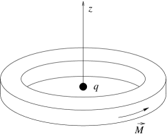
Figure 1: Magnetized ring

X.1 Violation of the CMMT

As a second illustration of our discussion MedandSa , consider a ring with the shape of a washer made of a ferromagnetic insulator (see Fig. 1). The axis of the ring is along the $z$-axis and the center is at the origin. For simplicity we take $\epsilon=1$. The ring is magnetized around its axis with magnetization $\mathbf{M}$ of uniform magnitude. In this situation $\mathbf{B}=4\pi\mathbf{M}$ inside the ring whereas $\mathbf{H}=0$ everywhere. Suppose that at the center of the ring there is a particle of charge $q$. Since the ring is an insulator the electrostatic field of the charge penetrates the magnet. The total momentum defined by $T_{\mathrm{F}}^{\mu\nu}$ does not vanish but points in the $z$ direction. Using cylindrical coordinates $(\rho,\theta,z)$, $\mathbf{M}=M\hat{\mathbf{{\theta}}}$ and $\mathbf{r}=\rho\hat{\bm{{\rho}}}+z\hat{\mathbf{z}}$ we have

$$\mathbf{g}=\frac{1}{4\pi c}\mathbf{D}\times\mathbf{B}=\frac{qM}{cr^{3}}(-z\hat{\bm{\rho}}+\rho\hat{\mathbf{z}})\ .$$ (226)

and integrating over the volume

$$\mathbf{p}=\frac{qM}{c}\int dV\,\frac{\rho}{r^{3}}\,\hat{\mathbf{z}}\ .$$ (227)

The center of mass of the system (including the electromagnetic contribution to the energy) is at rest at the center of the ring. Then the usual CMMT is violated. Note that Abraham’s momentum density vanishes since $\mathbf{H}=0$, so that if one takes it to define the momentum of the electromagnetic field, the total momentum of the system including the electromagnetic field is zero.

Let us now examine what happens when the fields change by considering the scenario in which the washer demagnetizes (e. g.  by the action of a device included in the magnet which allows its temperature to rise above the Curie point). The magnetic induction field $\mathbf{B}$ changes and therefore an induced electric field appears. It is always possible to split the electric field in a static field, $\mathbf{E}_{S}$, $\nabla\cdot\mathbf{E}_{S}=4\pi\rho$, $\nabla\times\mathbf{E}_{S}=0$ and an induced field $\mathbf{E}_{\mathrm{I}}$, $\nabla\cdot\mathbf{E}_{\mathrm{I}}=0$, $\nabla\times\mathbf{E}_{\mathrm{I}}=-c^{-1}\dot{\mathbf{B}}$. It is easily shown that

$$\mathbf{E}_{\mathrm{I}}=-\frac{1}{4\pi c}\int dV\,\frac{\partial\mathbf{B}}{\partial t}\times\frac{\hat{\mathbf{r}}}{r^{2}}\ .$$ (228)

Neglecting the radiation field $\mathbf{B}=4\pi\mathbf{M}$. Then at the origin the induced field is

$$\mathbf{E}_{\mathrm{I}}(0)=-\frac{\dot{M}}{c}\int dV\,\frac{\rho}{r^{3}}\,\hat{\mathbf{z}}\ .$$ (229)

If the demagnetization process is fast enough, the force on the charge is $\mathbf{F}=q\mathbf{E}_{\mathrm{I}}(0)$, and the impulse on the (dressed) particle may also be computed

$$\mathbf{I}_{\mathrm{Charge}}=\int dt\,\mathbf{F}=-\frac{q}{c}\int dt\,\dot{M}\,\int dV\,\frac{\rho}{r^{3}}\,\hat{\mathbf{z}}\ .$$ (230)

Note that no $\mathbf{B}$ field is produced during the demagnetization process by the charge and there is no force acting on the magnet which therefore remains at rest. The mechanical momentum of the system is now different from zero. If one uses Abraham’s momentum density, the unavoidable conclusion is that momentum is not conserved. But on the other hand, (230) is exactly the momentum of the initial configuration calculated (227) using Minkowski’s momentum density, which is then shown to be consistent with momentum conservation. Since the center of mass of the magnet does not move, the center of mass of the system moves in the direction in which the particle moves with velocity

$$\dot{X}_{\mathrm{T}}^{i}=\frac{c^{2}}{U}p^{i}$$ (231)

where $U$ is the total rest energy of the system. The CMMT is again violated.

X.2 The motion of the center of mass and spin

The result obtained is nevertheless consistent with our center of mass and spin motion theorem (8). To see this we note that in the initial situation the total spin density satisfies again (217). For the temporal components we have,

$$\partial_{\alpha}S^{0i\alpha}=\tau^{0i}=(\mathbf{M}\times\mathbf{E})^{i}\ ,$$ (232)

and using again that matter is at rest we are left with

$$S^{0i0}=c(\mathbf{M}\times\mathbf{E})^{i}t+C_{1}$$ (233)

with $C_{1}$ a constant. Integrating over space and using $\mathbf{B}=4\pi\mathbf{M}$ we obtain

$$\dot{X}_{\theta}^{i}=\dot{X}_{\mathrm{S}}^{i}=-\frac{d}{dt}\frac{c}{U}S^{0i}=\frac{c^{2}}{U}p^{i}\ ,$$ (234)

in agreement with (8) and (231). There is a short period when the magnetization varies for which both $\dot{\mathbf{X}}_{\mathrm{T}}$ and $\dot{\mathbf{X}}_{\mathrm{S}}$ are variable.

X.3 Storing momentum in the magnet

To complete the picture, let us investigate the origin of the momentum that in ours and Minkowski’s formulation is stored in the electromagnetic field. Let us start with the charge far away and analyze how, as it is brought to the center of the ring, the field momentum builds up. The magnet does not produce an electromagnetic field outside itself. Hence there is no force acting upon the charge. There is, though, a force acting on the magnet produced by the magnetic field $\mathbf{B}$ generated as the charge moves. To keep the magnet in place an opposite force must be applied to it. The impulse generated by this force is precisely the stored momentum in the electromagnetic field. For a charge moving along the $z$-axis the calculation can be done easily.

Let us call $\mathbf{x}$ the position of the charge, $\mathbf{x}=\zeta\hat{\mathbf{z}}$. The velocity is $\mathbf{v}=\dot{\zeta}\hat{\mathbf{z}}$. For $v\ll c$ the magnetic field produced by the moving charge is

$$\mathbf{B}=\frac{q}{c}\frac{\mathbf{v}\times\mathbf{r}^{\prime}}{{r^{\prime}}^{3}}=\frac{q\dot{\zeta}\rho\hat{\bm{\theta}}}{c[\rho^{2}+(z-\zeta)^{2}]^{3/2}}\ ,$$ (235)

where ${\mathbf{r}}^{\prime}=\mathbf{r}-\mathbf{x}=\rho\hat{\bm{\rho}}+(z-\zeta)\hat{\mathbf{z}}$. Using (126), the force density on the magnet is

$$\mathbf{f}=M_{k}\nabla B_{k}=\frac{q}{c}\dot{\zeta}M\left[\hat{\bm{\rho}}\frac{\partial}{\partial\rho}+\hat{\mathbf{z}}\frac{\partial}{\partial z}\right]\frac{\rho}{{r^{\prime}}^{3}}\ .$$ (236)

The force is obtained by integrating over the volume

$$\mathbf{F}=\int dV\,\mathbf{f} = \frac{q}{c}\dot{\zeta}M\int dV\,\frac{\partial}{\partial z}\frac{\rho}{{r^{\prime}}^{3}}\,\hat{\mathbf{z}}$$ (237)

$$= -\frac{q}{c}M\frac{d}{dt}\int dV\,\frac{\rho}{{r^{\prime}}^{3}}\,\hat{\mathbf{z}}\ .$$ (238)

We have used $\partial_{z}=-\partial_{\zeta}$. The impulse on the magnet is then

$$\mathbf{I}_{\mathrm{Magnet}}=\int dt\,\mathbf{F}=-\frac{q}{c}M\int dV\,\frac{\rho}{r^{3}}\,\hat{\mathbf{z}}\ .$$ (239)

The momentum stored by the field is the opposite of this quantity and again agrees with (227). Also in this situation CMMT does not hold. If no external force is applied to keep the magnet in place, the charge would move with constant velocity but the magnet would be accelerated in the negative direction of the $z$ axis, as the center of mass would be too.

X.4 Toroidal currents

Figure 2: Toroidal currents

Taylor Taylor1965 has treated a related example, with toroidal currents instead of a magnet. It is interesting to have a view on the differences with our discussion in the starting situation with the charge at rest in the center. In this case the proper energy-momentum tensor is known to be the standard tensor defined in the vacuum, which is symmetric, $\mathbf{S}=c^{2}\mathbf{g}=c\mathbf{E}\times\mathbf{B}/4\pi$, and therefore CMMT holds. If one considers a free current distribution of value $\mathbf{j}=c\nabla\times\mathbf{M}$, with $\mathbf{M}$ the magnetization of our previous example, the magnetic induction field and the induced electric field are the same as in that case and the electromagnetic momentum density is equal to the one obtained using Minkowski’s expression in that situation. But now unlike in the magnet configuration the Poynting vector does not vanish. The force exerted on the currents by $\mathbf{E}$ is still zero, but the power density $\mathbf{E}\cdot\mathbf{j}$ is not, see Fig. 2. In the equivalent situation to the one discussed above, inside the structure that supports the currents, the energy is increasing in the top, and decreasing in the base. The total power does vanish. Since the force is zero, the velocity of the supporting structure maintains its null value; nevertheless, its center of mass moves because the internal energy is transported by Poynting’s vector from the bottom to the top. The CMMT imposes that the velocity of the center of mass should equal the stored momentum divided by the total energy. This makes this configuration ephemeral. Even disregarding Joule’s effect it could last only until the energy storage in the base is depleted. Regretfully, the analysis presented in Taylor’s paper is not correct because it does not take into account adequately the electromagnetic momentum. The energy transport mechanism just described is in contrast to what occurs with the magnet where the power density and the Poynting vector are zero. For this reason, the center of mass of the magnet may remain at rest.

XI Angular momentum of a magnetized cylinder

In our last illustration we consider the implications of the momentum density expression to orbital angular momentum equilibrium. Let us consider an infinite hollow cylinder made of a ferromagnetic insulating material with $\epsilon=1$ (see figure 3).

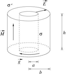
Figure 3: Magnetized hollow cylinder

The radius of the concentric hole is $a$ and the external radius is $b$. The cylinder is magnetized along its axis with a uniform magnetization $\mathbf{M}$. In the surface of the hole there is a uniform surface charge density $\sigma$ and in the external surface of the cylinder there is a cylindrical shell of insulator charged with a surface density $\sigma^{\prime}=-\sigma a/b$. In this condition inside the wall of the cylinder there is a uniform magnetic field $\mathbf{B}=4\pi\mathbf{M}$ and a radial electrostatic field

$$\mathbf{E}=4\pi\sigma\frac{a}{r}\hat{\mathbf{r}}\quad\hbox{for}\quad a<r<b$$ (240)

and $\mathbf{E}=0$ otherwise. The momentum density is

$$\mathbf{g}=\frac{1}{4\pi c}\mathbf{D}\times\mathbf{B}=-\frac{4\pi M\sigma a}{cr}\hat{\bm{\theta}}\ ,\qquad a<r<b\ .$$ (241)

Since $\mathbf{g}$ circulates around the axis there is a net orbital angular momentum $\mathbf{L}$ stored in the electromagnetic field. For a section of cylinder of height $h$ the angular momentum is

$$\mathbf{L}=\int\mathbf{r}\times\mathbf{g}\,dV=-\frac{(2\pi)^{2}}{c}M\sigma a(b^{2}-a^{2})h\hat{\mathbf{z}}\ .$$ (242)

Note that the EM fields store angular momentum although macroscopically there is nothing rotating.

If the cylinder demagnetizes an induced electric field is generated. The field produces a torque on the charged shell and the angular momentum is transferred to the shell. For $a<r\leq b$ the induced electric field is

$$\mathbf{E}_{\mathrm{i}n}=-\frac{2\pi}{cr}(r^{2}-a^{2})\dot{M}\hat{\bm{\theta}}$$ (243)

and the torque on the shell is

$$\bm{\tau}=\int\mathbf{r}\times\mathbf{E}_{\mathrm{i}n}\sigma^{\prime}dS=\frac{(2\pi)^{2}}{c}\sigma a(b^{2}-a^{2})h\dot{M}\hat{\mathbf{z}}\ .$$ (244)

The angular impulse is indeed equal to the angular momentum of the electromagnetic fields,

$$\int\bm{\tau}\,dt=\mathbf{L}\ .$$ (245)

In this situation only Minkowski’s momentum density is consistent with angular momentum conservation. Abraham’s momentum density yields a null angular momentum in the initial situation since $\mathbf{H}=0$.

XII Conclusion

In this paper we attain a complete resolution of the Abraham-Minkowski controversy on the energy-momentum tensor of the electromagnetic field in matter by introducing a new energy-momentum tensor which is different from those previously proposed. Our approach emphasizes the local character of the force and the torque exerted by the field on matter and requires that the energy-momentum tensor be locally well determined. It cannot be arbitrarily modified by the addition of a divergence-less term, even if by doing so the total energy and momentum do not change.

Our discussion departs from the main lines of argumentation prevailing in the recent literature on the topic. It is based on four main points: First, the force density on matter is in principle a measurable quantity and should be computable as the divergence of the matter tensor. Momentum conservation determines in an unambiguous way the energy-momentum tensor of the electromagnetic field. Second, all terms which contribute to inertia, including those of electromagnetic origin, should be included in the matter tensor and consequently excluded from the electromagnetic one. Third, the force density should be compatible with the microscopic Lorentz force. Fourth, magnetization is a manifestation of spin and EM fields produce torques on polarized matter, hence a complete understanding of the mechanical behavior of polarizable matter in an electromagnetic field requires the dynamics of spin too.

In this work the necessity of a relativistic invariant description of the matter-field interaction and the understanding of the true consequences of such a description play a key role. Throughout the discussion we insisted on the idea that the polarizations tensor which includes the electric polarization and the magnetization in a relativistic covariant object, should be used to describe the polarization of matter. We avoid arguments that rely on the properties of the electric and magnetic permeabilities which are defined only in the rest frame of matter (which not always exist). As an element which has more general consequences we discuss the serious limitations of the CMMT, which does not take into account the contribution of spin to the dynamics. The uncritical use of the CMMT in this context has been the source of many confusions and even mistakes in previous papers on this subject.

The conditions imposed on the form of the force density on matter by the relativity principle, the validity of Maxwell’s microscopic and macroscopic equations and the consistency with Lorentz microscopic force allow us to determine uniquely an expression of the force density on polarizable matter. This expression is similar but different to some of the expressions discussed in the past. The total force that the electromagnetic field exerts on an isolated sample of matter computed with our expression is the same as the total Lorentz force computed on the bound charges and currents of the sample. It is also equal to the total force predicted by the use of Minkowski’s tensor but it is different to the one consistent with Abraham’s tensor. The term known as Abraham’s force is not present in our formulation. Our analysis of the force density uncovers also the portion of the energy momentum tensor of matter which depends on the field. This includes the electrostatic potential energy of the dipoles, a momentum contribution required for the polarization of matter and, depending on the external conditions on matter, a field dependent mechanical response of matter which modifies its stress tensor.

The energy-momentum tensor of the field is fixed by the form of the force density and we are able to get its correct expression. The energy density of this tensor is not Poynting’s classic formula. It is shown to be the energy density of the electromagnetic field in vacuum minus the electrostatic energy of the dipoles. This term represents a electromagnetic contribution to inertia. Poynting’s vector maintains its interpretation as the energy density current once the correct expression of the power transmitted by the field to matter is taken into account. The momentum density is shown to be Minkowski’s expression. It is shown to be the momentum in vacuum minus the field dependent momentum of matter. This puts an end to the long standing controversy.

The energy-momentum tensor of the field is asymmetric. This has important consequences. This asymmetry is shown to be necessary for the coupling of the total spin density (magnetization) and the orbital angular momentum of matter. The asymmetry cancels exactly the effect of the torque density in the dynamical equation of the field spin density with the general result that the spin of the field is decoupled from the polarization of matter.

We presented a second approach to deduce the form of the electromagnetic energy-momentum tensor in matter. For this we perform a space-time average starting from the microscopic equations and postulate a monopolar and a dipolar coupling of matter with the macroscopic field. By imposing consistency with Maxwell’s equations we identify the monopolar current with the free charges, and show that the dipolar coupling is described by the polarization tensor in such a way that we recover exactly the formulation of the first approach. Although it may be foreseeable, this result has a deep meaning: Relativistic invariance and the physical hypotheses discussed in section V uniquely determine the equations of the macroscopic field up to the dipolar approximation. It will be interesting to investigate if the quadrupolar approximation maintains such robustness.

In our presentation, we also note that although in a general situation Minkowski’s tensor is not particularly useful, for a material with non-dispersive linear polarizabilities ($D_{\alpha\beta}=2^{-1}\chi_{\alpha\beta\mu\nu}F^{\mu\nu}$) it may be interpreted as the energy-momentum tensor of the electromagnetic field plus the fraction of the energy of matter arising from the polarization. Working with care it can be used in this case. Nevertheless its divergence is not the reaction of the force acting on matter. This explains the absence of magnetostriction and electrostriction in Minkowski’s approach. When an electromagnetic wave propagates on such a medium Minkowski’s tensor describes the whole wave and hence satisfies von Laue-Møller criterion.

The arguments presented in this paper are of theoretical nature. Of course, the ultimate test of the validity of our approach should be the direct measurement of the force density in different situations. For some of the experiments that have been done in the past, it is not completely straightforward to conciliate the measurements obtained with a definite choice of the force density or momentum expressions. In consequence there have been confronting opinions on how to interpret correctly the results of those experiments. Nevertheless there are some situations in which in our opinion our analysis proves to be clearly better. The applications and examples presented in the text were devised with this in mind.

In section V we discuss some of the implications of our approach for the analysis of the experiments which have been performed to determine the electromagnetic force density in matter. In particular we show that the result of the Walker, Ladhoz and Walker experiment, which is usually presented as an evidence for the existence of Abraham’s force term, may be better understood as a manifestation of the field dependent terms of the matter energy-momentum tensor. Our discussion of the electromagnetic forces on solid and liquid dielectrics strongly supports the validity of the force density that we are proposing.

We use our force density, the energy and momentum definitions obtained from $T^{\mu\nu}_{\mathrm{F}}$ and Maxwell’s equations to verify energy and momentum conservation in the interaction of a packet of electromagnetic waves with a dielectric medium. In opposition to the statement of the influential argument first advanced by Balazs Balazs1953 , that for sixty years has been considered a strong support in favor of Abraham’s point of view, we show that for $n>1$ the wave packet effectively pulls the material when it enters a medium (See Eq.(208)). This in fact is a most comfortable result after observing that it has a simple physical explanation. Dielectric and paramagnetic materials are attracted while diamagnetic materials are repelled in the direction to high field regions. When the wave packet is entering the medium it pulls the material unless diamagnetism prevails. For the same reason when the wave leaves, it drags the block forward. We complete our picture of this process by computing the evolution of the spin density. This calculation shows that the boost momentum gives the precise contribution necessary for our center of mass and spin to behave inertially.

The example of the charge-magnet system presented in section X, gives in a very simple setup an illustration of the consequences of the main ideas behind our formulation. In the same spirit, for the magnetized cylinder analyzed in section XI we show how our approach gives an appealing and consistent description of a system where the orbital angular momentum stored in the EM fields is transferred to matter.

As a by-product of the analysis presented in this paper the weakness of the CMMT was exposed in specific physical situations, and the validity of the improved theorem which includes the spin contributions was tested. These results also show that the hidden momentum hypothesis is unnecessary. Although we have not made a detailed check in each case (which would take a disproportionate effort), we think that the many analysis found in the literature which are based in this hypothesis should prove wrong or at least superfluous.

Our results open a range of theoretical and experimental possibilities of research in the study of the interaction of the electromagnetic fields with polarizable matter. Our construction of the force density suggests to make a methodological shift in the approach to the many applications in which it plays a role and concentrate in the determination of the physically acceptable polarization tensor of the system under study, preferably in the laboratory reference frame. This may be applied to a variety of systems, which include ionized gases, dielectric liquids, and non linear magnetic matter, to give a few examples. In the past these were either ignored or studied in terms of the permeabilities. We note that the polarization tensor of some of these systems may depend on the local velocity of matter, so that velocity dependent effects are not banned from our formulation. It is only Abraham’s like terms which are found unnecessary. On the experimental side the determination of force density instead of the total force advocated by some authors and in particular by Brevik Brevik1979 in the past acquires new importance. A critical reanalysis an even a remaking of the experiments which perform a direct measurement of the momentum of photon should be useful for establishing without further doubts Minkowski’s momentum as the classical and quantum momentum of light. Experiments exploring the inertiality of the center of mass and spin in this context which may include the real versions of the idealized situations discussed in sections IX, X and XI will also contribute to the complete experimental clarification of this subject.

Appendix A Energy and momentum of dressed dipoles

The time derivative terms that spoil the relativistic covariance in (113) and (114) actually correspond to part of the momentum and energy of the microscopic electromagnetic interaction. In addition to the external fields we considered in section V.3 there are also the electromagnetic fields produced by the dipolar system itself

$$\mathbf{E}_{\mathrm{t}} = \mathbf{E}+\mathbf{E}_{\mathrm{d}}\ ,$$ (246)

$$\mathbf{B}_{\mathrm{t}} = \mathbf{B}+\mathbf{B}_{\mathrm{d}}\ .$$ (247)

The energy density of the total electromagnetic field is

$$u_{\mathrm{t}}=u+u_{\mathrm{d}}+\frac{1}{4\pi}(\mathbf{E}\cdot\mathbf{E}_{\mathrm{d}}+\mathbf{B}\cdot\mathbf{B}_{\mathrm{d}})$$ (248)

and the momentum density is

$$\mathbf{g}_{\mathrm{t}} = \frac{1}{4\pi c}\mathbf{E}_{\mathrm{t}}\times\mathbf{B}_{\mathrm{t}}$$ (249)

$$= \mathbf{g}+\mathbf{g}_{\mathrm{d}}+\frac{1}{4\pi c}(\mathbf{E}\times\mathbf{B}_{\mathrm{d}}+\mathbf{E}_{\mathrm{d}}\times\mathbf{B})\ .$$

The integrals of the energy density $u_{\mathrm{d}}$ and of the momentum density $\mathbf{g}_{\mathrm{d}}$ that only depend on the dipolar fields $\mathbf{E}_{\mathrm{d}}$ and $\mathbf{B}_{\mathrm{d}}$ are part of the energy and momentum of the dressed dipole.

The interaction momentum and energy are the integrals over the whole space of products of an external field and a dipolar field. We assume that the the external fields are essentially constant where the dipolar system is located and that the fields of the dipolar system are well-approximated by the fields of dipolar moments where the external charges and currents are located (dipolar approximation). The integrals can be split in a local term corresponding to the region around the dipolar system and an external term outside this region,

$$\int_{\mathrm{whole-space}}{\dots}\,dV=\int_{\mathrm{local}}{\dots}\,dV+\int_{\mathrm{external}}{\dots}\,dV\ .$$ (250)

The local electromagnetic interaction energy and interaction momentum also contribute to the dressed dipole energy and momentum. The local interaction energy is

$$U_{\mathrm{i}}=\frac{1}{4\pi}\int_{\mathrm{local}}(\mathbf{E}\cdot\mathbf{E}_{\mathrm{d}}+\mathbf{B}\cdot\mathbf{B}_{\mathrm{d}})\,dV$$ (251)

and the local interaction momentum is

$$\mathbf{p}_{\mathrm{i}}=\frac{1}{4\pi c}\int_{\mathrm{local}}(\mathbf{E}\times\mathbf{B}_{\mathrm{d}}+\mathbf{E}_{\mathrm{d}}\times\mathbf{B})\,dV\ .$$ (252)

To evaluate the contribution of the local interaction terms we use the fact that the external fields are essentially constant. Then

$$U_{\mathrm{i}}\approx\frac{1}{4\pi}\left(\mathbf{E}\cdot\int\mathbf{E}_{\mathrm{d}}\,dV+\mathbf{B}\cdot\int\mathbf{B}_{\mathrm{d}}\,dV\right)\ ,$$ (253)

and

$$\mathbf{p}_{\mathrm{i}}\approx\frac{1}{4\pi c}\left(\mathbf{E}\times\int\mathbf{B}_{\mathrm{d}}\,dV+\int\mathbf{E}_{\mathrm{d}}\,dV\times\mathbf{B}\right)\ .$$ (254)

These approximations have a pitfall because the whole-space integrals of the dipolar fields are non-convergent improper integrals. Nevertheless, in the next appendix we argue that the physically consistent values of the integrals are

$$\int\mathbf{B}_{\mathrm{d}}\,dV=0$$ (255)

and

$$\int\mathbf{E}_{\mathrm{d}}\,dV=-4\pi\mathbf{d}\ .$$ (256)

Therefore

$$U_{\mathrm{i}}=-\mathbf{d}\cdot\mathbf{E}$$ (257)

and

$$\mathbf{p}_{\mathrm{i}}=-\frac{1}{c}\mathbf{d}\times\mathbf{B}\ .$$ (258)

As we have shown in subsection V.3, these contributions to the interaction, (258) and (257), exactly cancel the additional terms in (113) and (114). In other words (113) and (114) correspond to the force and power on the bare dipole while for the dressed dipole the offending terms are not present.

Appendix B Integrals of self fields of dipolar systems

In this section we prove that the whole-space volume integrals of the dipolar fields that appear in appendix A are non-convergent improper integrals. We show that the physically consistent values of these integrals are those given by (255) and (256). We assume that the external fields are $\mathbf{E}=-\nabla\phi$ and $\mathbf{B}=\nabla\times\mathbf{A}$ with the potentials vanishing at infinity as $1/r$. Near the dipolar system the fields are constant, then $\phi\approx\phi(0)-\mathbf{E}(0)\cdot\mathbf{x}$ and $\mathbf{A}\approx\mathbf{A}(0)+\mathbf{B}(0)\times\mathbf{x}/2$.

The integral of the self magnetic field on a finite volume $V$ is

$$\int_{V}\mathbf{B}_{\mathrm{d}}\,dV = \int_{V}\mathbf{B}_{\mathrm{d}}\cdot\nabla\mathbf{x}\,dV$$ (259)

$$= \int_{V}[\nabla(\cdot\mathbf{B}_{\mathrm{d}}\mathbf{x})-\nabla\cdot\mathbf{B}_{\mathrm{d}}\,\mathbf{x}]\,dV$$

$$= \oint_{\partial V}\mathbf{x}\,\mathbf{B}_{\mathrm{d}}\cdot d\mathbf{S}-\int_{V}\nabla\cdot\mathbf{B}_{\mathrm{d}}\,\mathbf{x}\,dV\,.\;$$

The surface integral is not convergent as the surface $\partial V$ goes to infinity. For example, for a sphere the surface integral is $(8\pi/3)\mathbf{m}$ regardless of the radius. Instead if the volume is taken as the doughnut-shaped figure whose surface is made of field lines then the integral vanishes.

Let us assume that there is some way of defining the limit that gives the “correct” physical value. Given the symmetry of the dipolar field the limit of the surface integral must be proportional to the dipole moment

$$\oint_{\partial V}\mathbf{x}\,\mathbf{B}_{\mathrm{d}}\cdot d\mathbf{S}\to\lambda\mathbf{m}\ .$$ (260)

Since $\nabla\cdot\mathbf{B}_{\mathrm{d}}=0$ the total integral is

$$\int\mathbf{B}_{\mathrm{d}}\,dV=\lambda\mathbf{m}\ .$$ (261)

The electrical case is quite similar. Since the magnetic and electric fields have the same form far away from the dipole, the surface integral must be the same for both fields.

$$\int\mathbf{E}_{\mathrm{d}}\,dV = \lambda\mathbf{d}-\int\nabla\cdot\mathbf{E}_{\mathrm{d}}\,\mathbf{x}\,dV$$ (262)

$$= \lambda\mathbf{d}-4\pi\int\rho\mathbf{x}\,dV$$

$$= \lambda\mathbf{d}-4\pi\mathbf{d}\ .$$

For determining the value of $\lambda$ let us calculate the whole interaction electric energy

$$\frac{1}{4\pi}\int\mathbf{E}\cdot\mathbf{E}_{\mathrm{d}}\,dV = -\frac{1}{4\pi}\int\nabla\phi\cdot\mathbf{E}_{\mathrm{d}}\,dV$$ (263)

$$= -\frac{1}{4\pi}\int[\nabla\cdot(\phi\mathbf{E}_{\mathrm{d}})-\phi\nabla\cdot\mathbf{E}_{\mathrm{d}}]\,dV$$

$$= \int\phi\rho\,dV$$

$$= -\mathbf{E}(0)\cdot\mathbf{d}\ ,$$

which of course is the electrostatic energy of the dipole and should be considered part of the energy of the dressed dipolar system. Therefore, it must be that $\lambda=0$. The integral of the magnetic field is then zero and there are not magnetic contributions to the momentum or energy of the dressed dipole. Nevertheless, the whole interaction magnetic energy is not zero,

$$\frac{1}{4\pi}\int\mathbf{B}\cdot\mathbf{B}_{\mathrm{d}}\,dV = \frac{1}{4\pi}\int\nabla\times\mathbf{A}\cdot\mathbf{B}_{\mathrm{d}}\,dV$$ (264)

$$= \frac{1}{4\pi}\int\mathbf{A}\cdot\nabla\times\mathbf{B}_{\mathrm{d}}\,dV$$

$$= \frac{1}{c}\int\mathbf{A}\cdot\mathbf{j}_{\mathrm{m}}\,dV$$

$$= \mathbf{B}(0)\cdot\mathbf{m}\ .$$

This energy must be assigned to the external system. If an external field $\mathbf{B}$ is turned on in a region where there is a constant magnetic dipole, a work $-\mathbf{B}\cdot\mathbf{m}$ is done on the bare dipole. The opposite is the work done on the external system.

References

- (1) H. Minkowski, Nachr. Ges. Wiss. Göttingen, 53, (1908).
- (2) M. Abraham, Rend. Circ. Mat. Palermo 28, 1–28, (1909).
- (3) M. Abraham, Rend. Circ. Mat. Palermo 30, 33–46, (1910).
- (4) A. Einstein and J. Laub, Ann. Phys. (Leipzig) 26, 532–540 (1908)
- (5) A. Einstein and J. Laub, Ann. Phys. (Leipzig) 26, 541–550 (1908)
- (6) F. Beck, Z. Phys. 134, 136–155 (1953).
- (7) G. Marx and G. Györgyi, Ann. Phys. (Leipzig) 16, 241–256 (1956).
- (8) S. R. de Groot and L. G. Suttorp, Foundations of Electrodynamics, North Holland, Amsterdam, 1972.
- (9) R. Peirls, Proc. Royal. Soc. A347, 475–491, (1976).
- (10) R. Peirls, Proc. Royal. Soc. A355, 141–151, (1977).
- (11) W. Shockley and R. P. James, Phys. Rev. Lett. 18, 876–879 (1967).
- (12) M. L. H. Pryce, Proc. Roy. Soc. 195, 62–81 (1948).
- (13) E. L. Hill, Rev. Mod. Phys. 23, 253–260 (1951).
- (14) C. L. Tang and J. Meixner, Phys. of Fluids 4, 148–154 (1961).
- (15) R. L. Dewar, Aus. J. Phys. 30, 533–575 (1977).
- (16) W. Israel, Phys. Lett. B67, 125–128 (1977).
- (17) M. Kranyš, Can. J. Phys. 57, 1022–1026 (1979).
- (18) G. Maugin, Can. J. Phys. 58, 1163–1170 (1978).
- (19) Robert N. C. Pfeifer et al, Rev. Mod. Phys. 79, 1197–1216 (2007).
- (20) Shin-tiro Goto, Robin W. Tucker and Timothy J. W. Alton, Proc. Royal. Soc. A467, 59–78, (2011)
- (21) James P. Gordon, Phys. Rev.A8, 14–21 (1973).
- (22) D. F. Nelson, Phys. Rev.A44, 3985–3996 (1991).
- (23) Stephen M. Barnett, Phys. Rev. Lett. 104, 070401 (2010).
- (24) F. J. Belinfante, Physica VI, 887–898 (1939).
- (25) L. Rosenfeld, Mem. Acad. Roy. Belg. (Cl. Sciences) 18,fasc. 6, 2–30 (1940).
- (26) W. Pauli, Rev. Mod. Phys. 13, 203–232 (1941).
- (27) Sidney Coleman and J. H. Van Vleck Phys. Rev. 171, 1370–1375 (1968).
- (28) M. v. Laue, Z. Physik 128, 387–394 (1950).
- (29) C. Møller, The theory of relativity, Oxford, (1952).
- (30) Rodrigo Medina and J. Stephany, Eur. J. Phys. 38, 015208 (8pp), (2017).
- (31) A. Papapetrou, Phil. Mag. 40, 937–946 (1949).
- (32) A. Einstein, W. J. de Haas, Deutsche Physikalische Gesellschaft, Verhandlungen 17, 152–170 (1915).
- (33) S. J. Barnett and G.S. Kenny, Phys. Rev. 91, 408–411 (1953).
- (34) Rodrigo Medina and J. Stephany, An improved inertia principle, arXive:1404.1590.
- (35) Rodrigo Medina and J. Stephany, Belinfante-Rosenfeld tensor and the inertia principle, arXiv:1404.3334.
- (36) J. H. Poynting, Phil. Trans. R. Soc. 175, 343–361 (1884).
- (37) L. Landau and E. Lifchitz, Classical theory of fields, Butterworth-Heinemann, Oxford, 1994, p. 87.
- (38) G. H. Livens, Phil. Mag. 32, 162–171 (1916).
- (39) W. Pauli, The theory of relativity, Pergamon, (1958).
- (40) D. V. Skobel’tsyn, Sov. Phys. Usp. 16, 381–401 (1973).
- (41) M. G. Burt and R. Peirls, Proc. Royal. Soc. A333, 149–156, (1973).
- (42) J. L. Synge, Hermathena, 117, 80–84, (1974).
- (43) F. N. H. Robinson, Phys. Rep. 16, 313–354 (1975).
- (44) V. L. Ginzburg and V. A. Ugarov, Sov.Phys.Usp. 19, 94-101 (1976).
- (45) I. Brevik, Phys. Rep. 52, 133–201 (1979).
- (46) R. Loudon, Fortschr. Phys. 52, 1134–1140 (1980).
- (47) U. Leonhart, Nature 444, 823–824 (2006).
- (48) Y. N. Obukhov, Ann. Phys.(Berlin) 17,830–851 (2008).
- (49) M. N. Novac, Fortschr. Phys. 28, 285–353 (1980).
- (50) Peter W. Milonni and Robert W. Boyd, Advances in Optics and Photonics 2, 519–553 (2010).
- (51) Stephen M. Barnett and Rodney Loudon, Phil. Trans. R. Soc. A 368, 927–939 (2010).
- (52) B. A. Kemp, J. Appl. Phys. 109, 111101 (2011).
- (53) Adrian Cho, Science 327 1067 (2013).
- (54) M. Abraham, Ann. Phys.(Leipzig) 44,537–543 (1914).
- (55) R. Grammel, Ann. Phys.(Leipzig) 41,570–580 (1913).
- (56) V. G. Veselago, V. V. Shchavlev, Physics–Uspekhi 53, 317–318 (2010).
- (57) Teodor M. Atanackovic and Ardéshir Guran, Theory of Elasticity for Scientists and Engineers, Birkhäuser, Boston, 2000, p. 11.
- (58) Yuan-cheng Fung and Pin Tong, Classical and Computational Solid Mechanics, World Scientific Publishing Co., Sigapore, 2001, pp. 75, 77–78.
- (59) N. L. Balazs, Phys. Rev. 91, 408–411 (1953).
- (60) E. G. Cullwick, Nature, 170, 425 (1952).
- (61) T. T. Taylor, Phys. Rev. 137, B467–B471 (1965).
- (62) W. H. Furry, Am. J. Phys. 37, 621–636 (1969).
- (63) D. Babson, S. P. Reynolds, R. Bjorkquist and D. J. Griffiths, Am. J. Phys. 77, 826–833 (2009).
- (64) P. Penfield Jr. and H. A. Haus, Electrodynamics of Moving Media MIT, Cambridge, MA, 1967.
- (65) H. A. Haus, Physica 43, 77-91 (1969).
- (66) R. Klíma and V. A.Petržílka, Ann.Phys.(NY) 92, 395–405 (1975).
- (67) K. Furutsu, Phys. Rev. 185, 257–272 (1969).
- (68) T. G. Philbin, Phys. Rev. A83, 013823 (2011).
- (69) Yuri N. Obukhov, Friedrich W. Hehl, Phys. Lett. A311, 277–284, (2003).
- (70) J. D. Jackson, Classical Electrodynamics 3rd ed., John Wiley&Sons, New York, 1998, p. 189, p. 213.
- (71) F. Rasetti, Phys. Rev. 66, 1–5, (1944).
- (72) D. J. Hughes and M. T. Burgy, Phys. Rev. 81, 498–506, (1951).
- (73) Rodrigo Medina, J. Phys. A: Math Gen 39, 3801–3816 (2006).
- (74) Rodrigo Medina, Am. J. Phys. 74, 1031–1034 (2006).
- (75) R. A. Beth, Phys. Rev. 50, 115–125 (1936).
- (76) N. Carrara, Nature 164, 882-883 (1949).
- (77) M. E. J. Friese, J. Enger, H. Rubinsztein-Dunlop, and N. R. Heckenberg, Phys. Rev. A54, 1593–1596 (1996).
- (78) M. E. J. Friese, T.A. Nieminen, H. Rubinsztein-Dunlop, and N. R. Heckenberg, Nature 394, 348–350 (1998).
- (79) Rodrigo Medina and J. Stephany, Electromagnetic fields in matter revisited arXiv:1404.5189
- (80) R. V. Jones and J. C. S. Richards, Proc. Roy. Soc. A221, 480–498 (1954).
- (81) R. V. Jones and B. Leslie, Proc. Roy. Soc. A360, 347–363 (1978).
- (82) A. F. Gibson, M. F. Kimmitt, A. O. Koohian, D. E. Evans and G. F. D. Levy, Proc. Royal. Soc. A370, 303–311, (1980)
- (83) G. K. Campbell, A. E. Leanhardt, Jongchul Mun, M. Boyd, E. W. Streed, W. Ketterle and D. E. Pritchard, Phys. Rev. Lett. 94, 170403 (2005).
- (84) V. S. Zuev and G. Ya. Zueva,Opt. and Spect. 106, 248–251. (2009).
- (85) V. L. Ginzburg, Sov. Phys. Usp. 2, 874–893 (1960).
- (86) V. L. Ginzburg, Theoretical physics and Astrophysics, Pergamon Press (1979).
- (87) Li Zhang, Weilong She, Nan Peng and Ulf Leonhardt, New J. Phys. 17, 053035 (2015).
- (88) Amir M. Jazayeri and Khashayar Mehrany, Phys. Rev. A89, 043845 (2014).
- (89) J. H. Poynting, Phil. Mag. 9, 393–361 (1905).
- (90) G. Barlow, Proc. Roy. Soc. A87, 1–16 (1912).
- (91) A. Ashkin and J. M. Dziedzic, Phys. Rev. Lett. 30, 139–142 (1973).
- (92) H. M. Lai and K. Young, Phys. Rev. A14, 2329-2333 (1976).
- (93) A. Casner and J. P. Delville, Phys. Rev. Lett. 87 054503 (2001).
- (94) K. Sakai,D. Mizuno and K. Takagi,Phys. Rev. E63 046302 (2001).
- (95) N. G. C. Astrath, L. C. Malacarne, M. L. Baesso, G. V. B.Lukasievicz and S. E. Bialkowski, Nat. Commun. 5, 4363 (2014).
- (96) V. Kajorndejnukul, Weiqiang Ding, S. Sukhov, Cheng-Wei Qiu and A. Dogariu, Nature Photon. 5, 1–4 (2011).
- (97) Cheng-Wei Qiu, Weiqiang Ding, M. R. C. Mahdy, Dongliang Gao, Tianhang Zhang, Fook Chiong Cheong, A. Dogariu, Zheng Wang and Chwee Teck Lim, Light: Sci. Appl. 4, e278, (2015).
- (98) G. B. Walker and D. G. Lahoz, Nature 253, 339–340 (1975).
- (99) G. B. Walker, D. G. Lahoz and G. Walker, Can.Jour.Phys. 53, 2577–2586 (1975).
- (100) G. B. Walker and G. Walker, Can.Jour.Phys. 55, 2121–340 (1977).
- (101) Weilong She, Jianhui Yu and Raohui Feng, Phys. Rev. Lett. 101, 243601 (2008).
- (102) G. L. J. A. Rikken and B. A. van Tiggelen, Phys. Rev. Lett. 108, 230402 (2012).
- (103) S. S. Hakim and J. B. Higham, Proc. Phys. Soc. 80, 190 (1962).
- (104) J. A. Stratton, Electromagnetic Theory, Mc Graw-Hill, New York, 1941, p. 140.
- (105) F. Richter and U. Lotter, Phys. Stat. 34 K149–K152 (1969).
- (106) I. Turek, J. Rusz, and M. Diviš, Czech. J. Phys. 54, D279 (2004).
- (107) M. D. James and D. Kinderlehrer, Phil. Mag. B 68, 237–274 (1993).
- (108) Ruqian Wu, J. Appl. Phys. 91, 7358–7360 (2002)
- (109) Rodrigo Medina and J. Stephany, The force density and the kinetic energy-momentum tensor of electromagnetic fields in matter arXiv:1404.5250
- (110) Rodrigo Medina and J. Stephany, Violation of the center of mass theorem for systems with electromagnetic interaction arXiv:1404.5251