Revisiting stochastic off-policy action-value gradients

Abstract

Off-policy stochastic actor-critic methods rely on approximating the stochastic policy gradient in order to derive an optimal policy. One may also derive the optimal policy by approximating the action-value gradient. The use of action-value gradients is desirable as policy improvement occurs along the direction of steepest ascent. This has been studied extensively within the context of natural gradient actor-critic algorithms and more recently within the context of deterministic policy gradients. In this paper we briefly discuss the off-policy stochastic counterpart to deterministic action-value gradients, as well as an incremental approach for following the policy gradient in lieu of the natural gradient.

1 Preliminaries

1.1 Stochastic off-policy theorem

Consider a Markov decision process (MDP), where an agent receives a reward, $r_{t}$, for an action, $a\in A$, taken in state, $s\in S$, according to some stochastic behavioral policy, $b:S$ x $A\rightarrow(0,1)$. We can acquire a target policy, $\pi_{\theta}$, that maximizes the cumulative rewards expected under this MDP by expressing its value as

$$J^{\pi}(\theta)=\mathbb{E}_{s\sim d^{b}}[V^{\pi}(s)]=\mathbb{E}_{s\sim d^{b},a\sim b}[\varphi^{\pi,b}Q^{\pi}(s,a)]$$ (1)

where $V^{\pi}(s)$ is the expected cumulative rewards starting from a given state, $s_{t}$, and $Q^{\pi}(s,a)$, the expected cumulative rewards, starting from said state with an action, $a_{t}$; then following the policy, $\pi_{\theta}$, until termination (Sutton & Barto, 2016). The importance sampling ratio, $\varphi^{\pi,b}$, scales $Q^{\pi}(s,a)$ according to the likelihood of sampling the undertaken action from $\pi_{\theta}$, rather than $b$. In order to find the parameters of $\pi_{\theta}$ such that the rewards are maximized, we can follow the direction of increasing performance

$$\nabla_{\theta}J^{\pi}(\theta) =\mathbb{E}_{s\sim d^{b},a\sim b}[\nabla_{\theta}\varphi^{\pi,b}Q^{\pi}(s,a)+\varphi^{\pi,b}\nabla_{\theta}Q^{\pi}(s,a)]$$ (2)

$$=\mathbb{E}_{s\sim d^{b},a\sim b}\bigg{[}\varphi^{\pi,b}\frac{\nabla_{\theta}\pi_{\theta}(a|s)}{\pi_{\theta}(a|s)}Q^{\pi}(s,a)\bigg{]}+\mathbb{E}_{s\sim d^{b},a\sim b}[\varphi^{\pi,b}\nabla_{\theta}Q^{\pi}(s,a)]$$ (3)

$$\approx\mathbb{E}_{s\sim d^{b},a\sim b}\bigg{[}\varphi_{\pi,b}\frac{\nabla_{\theta}\pi_{\theta}(a|s)}{\pi_{\theta}(a|s)}Q^{\pi}(s,a)\bigg{]}=\widetilde{\nabla}_{\theta}J^{\pi}(\theta)$$ (4)

The first term in the above equation is the off-policy gradient and the second term is the off-policy action-value gradient (Degris et al., 2012). We want to approximate the second term, so as to move in the policy gradient direction.

1.2 Deterministic action-value gradient

Action-value methods such as Q-learning acquire an implicit deterministic policy, $\mu_{\theta}$, that can be expressed as $a=\operatorname*{argmax}_{a}Q^{\mu}(s,a)$. However this not feasible under continuous action spaces. For such, the policy needs to be represented explicitly (Silver et al., 2014; Sutton & Barto, 2016).

In order to learn the parameters for a continuous deterministic policy, $\mu_{\theta}$, Silver et al. (2014) proposed following the gradient of the action-value, $\nabla_{\theta}Q^{\mu}(s,a)|_{a=\mu_{\theta}(s)}$, such that the temporal difference (TD) error is minimized (Lillicrap et al., 2016). Using the chain-rule, if $Q^{\mu}(s,a)$ is a compatible function, the gradient can be decomposed into the update equation

$$\theta_{t+1} =\theta_{t}+\alpha\mathbb{E}_{s\sim p^{\mu}}[\nabla_{\theta}\mu_{\theta}(s)\nabla_{a}Q^{\mu}(s,a)|_{a=\mu_{\theta}(s)}]$$ (5)

$$=\theta_{t}+\alpha\mathbb{E}_{s\sim p^{\mu}}[\nabla_{\theta}\mu_{\theta}(s)\nabla_{\theta}\mu_{\theta}(s)^{\top}\omega]$$ (6)

where $\nabla_{\theta}\mu_{\theta}(s)$ is the deterministic policy gradient and $\omega$ are the parameters of the action-value function that minimize the TD error. The above equation moves in the same direction as the policy gradient. We now discuss a similar case for stochastic policies.

2 Stochastic Off-policy action-value gradient

2.1 Compatible action-value functions

In order to estimate how the parameters of an explicit policy change with respect to $Q^{\pi}_{\omega}(s,a)$, the action-value needs to be compatible with whatever type of policy is being represented. To do this, we re-parametrize it as

$$Q^{\pi}_{\omega}(s,a)=A^{\pi}_{\omega}(s,a)+V^{\pi}_{\nu}(s)$$ (7)

where $A^{\pi}_{\omega}(s,a)$ is the advantage function of an action in a state and $V^{\pi}_{\nu}(s)$ is the value of that state (Baird, ). Due to the zero-mean property of compatible features (Sutton et al., 2000; Peters et al., 2005), $Q^{\pi}_{\omega}(s,a)$ by itself cannot serve as a compatible function and at the same time, a reliable estimator for cumulative expected rewards. In practice, $A^{\pi}_{\omega}(s,a)$ is made compatible with respect to the stochastic policy whilst $V^{\pi}_{\nu}(s)$ is used as a baseline. Following (Sutton et al., 2000), we represent the advantage function of a stochastic policy as $A^{\pi}_{\omega}(s,a)=\frac{\nabla_{\theta}\pi_{\theta}(a|s)}{\pi_{\theta}(a|s)}^{\top}\omega$.

2.2 Stochastic off-policy gradient

Given an action-value function, $Q^{\pi}_{\omega}(s,a)$, that is compatible with the stochastic policy, $\pi_{\theta}$, in a manner shown above, we can decompose the action-value gradient term in the complete off-policy gradient theorem into

$$\mathbb{E}[\varphi^{\pi,b}\nabla_{\theta}Q_{\omega}^{\pi}(s,a)|d^{b},b] =\mathbb{E}_{s\sim d^{b},a\sim b}[\varphi^{\pi,b}\nabla_{\theta}A_{\omega}^{\pi}(s,a)]$$ (8)

$$=\mathbb{E}_{s\sim d^{b},a\sim b}[\varphi^{\pi,b}\nabla_{\theta}\pi_{\theta}(a|s)\nabla_{\pi_{\theta}}A_{\omega}^{\pi}(s,a)]$$ (9)

$$=-\mathbb{E}_{s\sim d^{b},a\sim b}\bigg{[}\varphi^{\pi,b}\frac{\nabla_{\theta}\pi_{\theta}(a|s)}{\pi_{\theta}(a|s)}\frac{\nabla_{\theta}\pi_{\theta}(a|s)}{\pi_{\theta}(a|s)}^{\top}\omega\bigg{]}$$ (10)

where the squared log-likelihood gradients represent the Fishers information matrix, $G^{\pi}(\theta)$. Consider the following from Bhatnagar et al. (2009)

Lemma 1. The optimal parameters, $w^{\ast}$, for the compatible function of a stochastic policy, $\pi_{\theta}$, can be expressed as

$$\omega^{\ast}=G^{\pi}(\theta)^{-1}\widetilde{\nabla}_{\theta}J^{\pi}(\theta)$$ (11)

which represents the natural policy gradient (Amari, 1998; Kakade, 2002). Hence the above moves in the off-policy gradient direction as both squared terms in the action-value gradient cancel out.

3 Experimental results

We evaluate the performance of an actor-critic algorithm that follows the policy gradient based on the above equation. We compare this algorithm, Actgrad, alongside two other algorithms: the off-policy actor-critic (Offpac) and Q-learning (Qlambda). Experiments are performed on the Cart Pole and Lunar Lander environments provided in the Open AI gym (Brockman et al., 2016).

3.1 Details

The first task we consider, Cart Pole, is the task of balancing a pole attached atop a cart by an un-actuated joint. The goal is to apply a force, F, to either the right or left of the pole in order to keep it upright. For each time step the pole is upright, a reward of 1 is given.

Next we consider, Lunar Lander, the task of piloting a lander module through the lunar atmosphere and unto a landing pad at the center of the screen. The goal is to bring the spacecraft to rest by either doing nothing or firing the main, left or right engines. Bad landings incur negative rewards, as do firing the engines. However, larger rewards are given for smooth landings.

For Cart Pole, the state features are encoded using the Boxes method (Barto et al., 1983), while for Lunar Lander they are encoded using heuristics provided by Open AI. Agents were trained on the environments for 1500 & 700 episodes respectively, with the same training parameters & learning rates shared across them. On Cart Pole, training episodes ended after 250 time steps while on Lunar Lander, they ended after 500 time steps. Training was repeated for 10 trials on each environment and testing was performed for 100 episodes after each trial.

3.2 Results

We now present the training and test results for the evaluated algorithms on each environment.

Table 1: Average Test Results.

Agent	Cart Pole		Lunar Lander
	Rewards	Episodes Solved	Rewards	Episodes Solved
Offpac	214.56 $\pm$ 3.78	99.9%	152.89 $\pm$ 8.52	91.7%
Qlearning	167.12 $\pm$ 2.97	99.0%	109.30 $\pm$ 8.87	79.2%
Actgrad	209.18 $\pm$ 3.68	99.7%	109.46 $\pm$ 11.27	85.7%

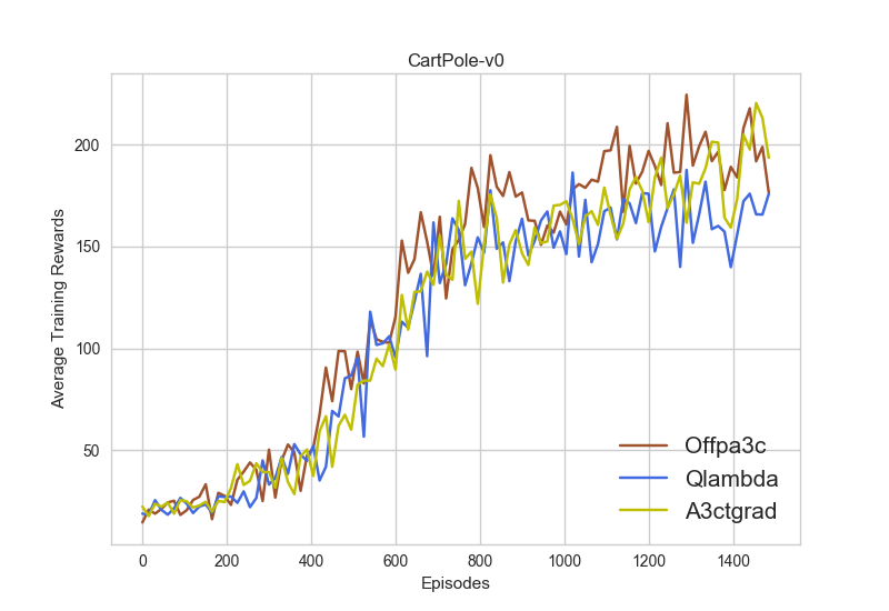
(a) Cart Pole.

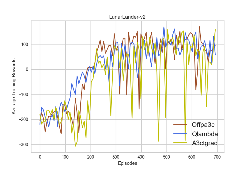
(b) Lunar Lander.

Figure 1: Average Training Rewards.

From the above, the investigated algorithm reaches a training performance close to that of the off-policy actor-critic on Cart Pole. However it suffers from higher variance on the Lunar Lander environment. This may be due to the fact that learning relies on estimates of the advantage as determined by the current advantage parameters, rather than the actual advantage gotten from the critic. This is likely pronounced due to the difficulty of Lunar Lander in comparison to Cart Pole.

4 Discussion

In this paper, we have discussed a method for following the stochastic off-policy gradient in a manner similar to that of the deterministic policy gradient. We then compared the performance of such method with other policy gradient algorithms. Although the approach suffers from high variance on certain tasks, it nevertheless outperforms deterministic algorithms and can easily be made to follow the steepest ascent direction by dropping the natural gradient term.

References

- Amari (1998) S. Amari. Natural gradient works efficiently in learning. In Neural Computation 10(2), pp. 251–276. 1998.
- (2) L. Baird. Advantage updating. Technical report, Wright-Patterson Air Force Base.
- Barto et al. (1983) A. Barto, R. Sutton, and C. Anderson. Neuronlike adaptive elements that can solve difficult learning control problems. In IEEE Transaction on Systems, Man and Cybernetics, pp. 2471–2482. 1983.
- Bhatnagar et al. (2009) S. Bhatnagar, R. Sutton, M. Ghavamzadeh, and M. Lee. Natural actor-critic algorithms. In Automatica 45, pp. 2471–2482. 2009.
- Brockman et al. (2016) G. Brockman, V. Cheung, L. Pettersson, J. Schneider, J. Schulman, J. Tang, and W. Zaremba. Open ai gym. arXiv:1606.01540, 2016.
- Degris et al. (2012) T. Degris, M. White, and R. Sutton. Off-policy actor-critic. In 29th International Conference on Machine Learning, 2012.
- Kakade (2002) S. Kakade. A natural policy gradient. In Advances in Neural Information Processing Systems 14. 2002.
- Lillicrap et al. (2016) T. Lillicrap, J. Hunt, N. Heess, A. Pritzel, N. Heess, T. Erez, Y. Tassa, D. Silver, and D. Wierstra. Continuous control with deep reinforcement learning. In 4th International Conference on Learning Representations, 2016.
- Peters et al. (2005) J. Peters, S. Vijayakumar, and S. Schaal. Natural actor-critic. In 16th European Conference on Machine Learning, 2005.
- Silver et al. (2014) D. Silver, G. Lever, N. Heess, T. Degris, D. Wierstra, and M. Riedmiller. Deterministic policy gradient algorithms. In 31st International Conference on Machine Learning, 2014.
- Sutton & Barto (2016) R. Sutton and A. Barto. Reinforcement Learning: An Introduction. The MIT Press, 2 edition, 2016.
- Sutton et al. (2000) R. Sutton, D. McAllester, S. Singh, and Y. Mansour. Policy gradient methods for reinforcement learning with function approximation. In Advances in Neural Information Processing Systems 12, pp. 1057–1063. 2000.
- Williams (1992) R. Williams. Simple statistical gradient-following algorithms for connectionist reinforcement learning. In Machine Learning, pp. 229–256. 1992.