Bloch-Siegert Shift and its Kramers-Kronig Pair

Abstract

We report that the Bloch-Siegert shift which appears in Nuclear Magnetic Resonance (NMR) spectroscopy can also be shown to originate as a part of a complex drive-induced second-order susceptibility term. The shift terms thus obtained are shown to have an absorptive Kramers-Kronig pair. The theoretical treatment involves a finite time-propagation of a nuclear spin-$1/2$ system and the spin-bearing molecule under the action of thermal fluctuations acting on the latter. The finite propagator is constructed to account for many instances of thermal fluctuations occurring in a time-scale during which the spin density matrix changes infinitesimally. Following an ensemble average, the resulting quantum master equation directly yields a finite time-nonlocal complex susceptibility term from the external drive, which is extremely small but measurable in solution-state NMR spectroscopy. The dispersive part of this susceptibility term originating from the non-resonant component of the external drive results in the Bloch-Siegert shift. We have verified experimentally the existence of the absorptive Kramers-Kronig pair of the second-order shift term, by using a novel refocussed nutation experiment. Our method provides a single approach to explain both relaxation phenomena as well as Bloch-Siegert effect, which have been treated using non-concurrent techniques in the past.

I Introduction

The question that how does a spin system behave in the presence of an external drive while being connected to a thermal bath, has been investigated in several notable works, spanning a few decades. A variety of different approaches exists in present literature, to deal with different aspects of this problem, which can be classified into two broad categories. To explain the phenomena of relaxation and nutation one adopts a quantum master equation approach akin to Wangsness and Bloch, where only the first order effects of the resonant part of a weak external drive is considered wangblo53 . Similar approaches involve the operation of moving to a doubly-rotating tilted frame before deriving the master equation as prescribed by Abragam, Vega and Vaughan et. al., or a heuristic assumption of independent rates of variation induced by the drive and the relaxation terms with a master equation only for the latter abragam06 ; vega1978 ; cotandurogryn04 . In all these approaches, the effect of the non-resonant (counter-rotating) part of an external drive is ignored. On the contrary, an important feature of the dynamics of such spin systems is the Bloch-Siegert shift, first reported in a detailed treatment by Siegert and Bloch, where the counter-rotating (or non-resonant) terms of the external drive produces a small shift in the resonance frequency by a factor proportional to $B_{1}^{2}$, with $B_{1}$ defined as amplitude of the drive field blochsiegert1940 . Such shifts follow from some form of perturbation due the external drive while ignoring the relaxation effects. Later approaches like the Floquet, Magnus or Average Hamiltonian Theory (AHT) and Fer expansion schemes all employ a perturbative treatment of the drive while neglecting the relaxation terms shirley1965 ; haeberlen1976 ; madhu2006 .

In this work, we strive to develop a single approach whereby both the resonant and the non-resonant part of a weak drive as well as the relaxation Hamiltonian, can be treated perturbatively for a spin-$1/2$ system coupled to a thermal bath undergoing rapid fluctuations. It is expected that the fluctuations would be present in a heat bath irrespective of the presence of the coupled spins or in other words, the molecules will undergo collisions irrespective of whether they bear a spin or not. Hence, we introduce a separate Hamiltonian which solely acts on the bath as a model of these fluctuations. We use the method of coarse-graining in time and finite propagation under all relevant Hamiltonians so as to realize the fact that in the timescales of the dynamics of the spin system, many instances of the fluctuations take place. We find that under these assumptions both the resonant and non-resonant parts of the drive can be treated perturbatively and the Bloch-Siegert shift naturally emerges as a second order perturbative correction. More precisely, both the resonant and non-resonant parts of the drive yield finite, albeit small, second order correction terms in the form of complex susceptibilities. While the dominant contribution of the imaginary (dispersive) part of the susceptibility term takes the form of Bloch-Siegert shift in an asymptotic limit, its Kramers-Kronig pair yields a decay term. We also note that in the absence of the coupling to the bath, we recover the expected unitary dynamics of the spins.

Since the Bloch-Siegert shift is well-studied, we experimentally verify the existence of the absorptive or the decay term obtained in our method. This effect is extremely small, and is usually overshadowed by the drive inhomogeneities. We remove the inhomogeneities by using a novel refocussing scheme to detect the presence of this additional decay due to the external drive, in agreement with our theoretical estimates.

II Description of the problem

We describe the problem in the context of solution-state nuclear magnetic resonance spectroscopy, but the arguments can easily be generalized to other quantum systems coupled to a thermal bath through a finite set of degrees of freedom. We envisage an ensemble of spin-$1/2$ nuclei and their respective spin-bearing molecules immersed in a thermal bath (a liquid solution at a fixed temperature $T$, or inverse temperature $\beta$). The nuclear spins (henceforth referred to as system) interact with the environment i.e. the bath through the spatial coordinates of the molecules which cradle the nuclear spins. The molecules are subjected to thermal collisions with other molecules in the solution. The entire solution is placed in a static, homogeneous, magnetic field $\bm{B}_{\circ}$ having magnitude $B_{\circ}$, the direction of which is chosen to define our $\hat{z}$ axis. In the limit of having a thermodynamically large number of spins immersed in the bath, the ensemble average of the spin-observables is to be understood as the average contribution of all spin-bearing molecules present in the bath.

II.1 Hamiltonians and their timescales

A single spin and its cradle i.e. the molecule (henceforth referred to as lattice) are described by the following Hamiltonian in the laboratory frame, in the units of angular frequency:

$$\mathcal{H}(t)=\mathcal{H}^{\circ}_{\scriptscriptstyle\rm S}+\mathcal{H}^{\circ}_{\scriptscriptstyle\rm L}+\mathcal{H}_{\scriptscriptstyle\rm SL}+\mathcal{H}_{\scriptscriptstyle\rm S}(t)+\mathcal{H}_{\scriptscriptstyle\rm L}(t),$$ (1)

where the individual Hamiltonians, their nature and the relevant timescales are described below.

• $\mathcal{H}^{\circ}_{\scriptscriptstyle\rm S}$: Zeeman Hamiltonian of the spin-magnetic field (static) coupling. $\mathcal{H}_{\scriptscriptstyle\rm S}^{\circ}=\omega_{\circ}I_{z}$, where $\omega_{\circ}=-\gamma B_{\circ}$ is the Larmor frequency and $\gamma$ is the gyromagnetic ratio of the spin-$1/2$ nuclei while $I_{\scriptscriptstyle\rm\alpha}$, $\alpha\in\{x,y,z\}$ denote the Cartesian components of the spin-$1/2$ angular momentum operator. $\omega_{\circ}$ is usually of the order of 100s of M-rad/s.

• $\mathcal{H}^{\circ}_{\scriptscriptstyle\rm L}$: Time-independent Hamiltonian of the cradle (or the spin-bearing molecule). Since only rotational degrees of freedom are relevant, this Hamiltonian reflects the molecular rotational energy eigen-system. Rotational (i.e. lattice) degrees of freedom of the ensemble of spin-bearing molecules is assumed to be in equilibrium with the thermal bath at an inverse temperature $\beta$. This Hamiltonian helps define the thermal equilibrium of the molecular rotational part through the equilibrium density matrix $\rho_{\scriptscriptstyle\rm L}^{\rm eq}=\frac{e^{-\beta\mathcal{H}^{\circ}_{\scriptscriptstyle\rm L}}}{\mathcal{Z}_{\scriptscriptstyle\rm L}}$, where, $\mathcal{Z}_{\scriptscriptstyle\rm L}$ is the partition function.

• $\mathcal{H}_{\scriptscriptstyle\rm S}(t)$: External transverse drive to the spin system, given by $\mathcal{H}_{\scriptscriptstyle\rm S}(t)=2\omega_{1}I_{\scriptscriptstyle\rm x}\cos(\omega t)$, where $2\omega_{1}=-\gamma B_{1}$ is the amplitude of the drive Hamiltonian while $\omega$ is its frequency. Subsequent analysis will assume a constant $\omega_{1}$, usually within the range of 1 - 100s of kilo-rad$/$s and a constant modulation frequency $\omega$. However, our analysis can easily be generalized to $\omega_{1}(t)$ which is an arbitrary function of time, provided $\omega_{1}(t)$ is sufficiently slowly varying compared to the lattice dynamics. $\omega_{1}/\omega_{\circ}\sim 10^{-3}$ implying that the spin quantum numbers act as good quantum numbers and in principle, $\mathcal{H}_{\scriptscriptstyle\rm S}(t)$ can be treated as a perturbation.

• $\mathcal{H}_{\scriptscriptstyle\rm SL}$: Coupling between the spin and the molecular spatial coordinates. It is usually assumed to be time-independent in the laboratory frame and involves operators of both spin and molecular (spatial) coordinates. We use a generic form of the coupling Hamiltonian as described by Wangsness and Bloch wangblo53 . Its amplitude is denoted by $\omega_{\scriptscriptstyle\rm SL}$. We assume a weak coupling to the lattice i.e. $\omega_{\scriptscriptstyle\rm SL}/\omega_{\circ}\ll 1$.

• $\mathcal{H}_{\scriptscriptstyle\rm L}(t)$: Fluctuations in the lattice. It embodies the effect of thermal collisions experienced by the spin-bearing molecule. Time-scales associated with this process are of the order of the time scale of molecular collisions which is less or equal to the rotational correlation time in liquids (of the order of a few picoseconds samidor85 ; tanabe78 ; gilgri72 ). The exact form of these processes can be quite complicated in the time scales of molecular collisions, but we adopt a simplified model based on the properties of the thermal equilibrium as described in the following paragraphs.

We model the term due to molecular collisions, $\mathcal{H}_{\scriptscriptstyle\rm L}(t)$ as stochastic fluctuations of the rotational energy levels (energy levels of $\mathcal{H}^{\circ}_{\scriptscriptstyle\rm L}$). Since the fluctuations do not drive the lattice away from equilibrium, we choose $\mathcal{H}_{\scriptscriptstyle\rm L}(t)$ to be diagonal in the eigen-basis $\{|\phi_{j}\rangle\}$ of $\mathcal{H}^{\circ}_{\scriptscriptstyle\rm L}$, represented by $\mathcal{H}_{\scriptscriptstyle\rm L}(t)=\sum_{j}f_{j}(t)|\phi_{j}\rangle\langle\phi_{j}|$. $f_{j}(t)$-s are assumed to be independent, Gaussian, $\delta$-correlated stochastic variables with zero mean and standard deviation $\kappa$.

We note that the fluctuations $\mathcal{H}_{\scriptscriptstyle\rm L}(t)$, which solely act on the lattice, may assume different values for different ensemble members at different time instants, while respecting the constraints imposed by the requirement of sustained thermal equilibrium. On the contrary, the other terms in the Hamiltonian (1) are identical for all ensemble members.

Starting with this description, we perform all subsequent calculations in the interaction representation of $\mathcal{H}^{\circ}_{\scriptscriptstyle\rm S}+\mathcal{H}^{\circ}_{\scriptscriptstyle\rm L}$ and all Hamiltonians in this representation are denoted by $H$ with relevant subscripts. Since $\mathcal{H}_{\scriptscriptstyle\rm L}(t)$ commutes with $\mathcal{H}^{\circ}_{\scriptscriptstyle\rm L}$ at all times, the form of the lattice fluctuations remain unchanged in the interaction representation.

In the interaction representation, let $\rho_{\scriptscriptstyle\rm S}(t)$ denote the density matrix of the spin-$1/2$ ensemble and $F(t)$ denote any arbitrary spin-observable for this ensemble. The dynamics of the expectation value of $F(t)$, denoted by $M(t)=\text{Tr}_{\scriptscriptstyle\rm S}\big{[}F(t)\rho_{\scriptscriptstyle\rm S}(t)\big{]}$ is given by

$$\frac{d}{dt}M(t)=\text{Tr}_{\scriptscriptstyle\rm S}\Big{[}\Big{\{}\frac{d}{dt}F(t)\Big{\}}\rho_{\scriptscriptstyle\rm S}(t)\big{]}+\text{Tr}_{\scriptscriptstyle\rm S}\Big{[}F(t)\Big{\{}\frac{d}{dt}\rho_{\scriptscriptstyle\rm S}(t)\Big{\}}\Big{]},$$ (2)

where, $\text{Tr}_{\scriptscriptstyle\rm S}$ denotes the trace over the spin-degrees of freedom. Since the spins are coupled to their respective molecules, $\rho_{\scriptscriptstyle\rm S}(t)$ is obtained from the full density matrix of the spin-molecule ensemble, $\rho(t)$ by tracing over the lattice degrees of freedom (denoted by $\text{Tr}_{\scriptscriptstyle\rm L}$). Hence in order to evaluate the r.h.s. of equation (2) we need a suitable expression for $\frac{d}{dt}\rho_{\scriptscriptstyle\rm S}(t)$, which is obtained from a quantum master equation, derived for the Hamiltonian $\mathcal{H}(t)$. In the following sections we derive such a master equation and explicitly show the dynamical equations relevant in the context of solution state NMR spectroscopy of an ensemble of spin-$1/2$ nuclei.

III Master equation with finite propagation for fluctuations

We seek to derive a master equation which captures the dynamics of the spin system described in the previous section. Since our problem concerns a single Hilbert space, a part of which undergoes rapid fluctuations we follow the standard practice of, (i) propagating for a large enough time $\Delta t\;(>0)$ over which fluctuations can be adequately averaged out, yet in the same interval $H_{\scriptscriptstyle\rm S}$ and $H_{\scriptscriptstyle\rm SL}$ should remain linearizable as is uasually done, (ii) taking ensemble average and a trace over the lattice variables and (iii) finally using the coarse-grained equation thus obtained as our dynamical equation with coarse-grained time derivatives replaced by ordinary ones cotandurogryn04 . The step (i) requires that the system and the fluctuations have widely separated timescales of evolution i.e. $\tau_{c}\ll\omega_{\scriptscriptstyle\rm 1}^{-1},\omega_{\scriptscriptstyle\rm SL}^{-1}$, where $\tau_{\scriptscriptstyle\rm c}$ is the time during which the lattice correlations are significant, such that we can find a $\Delta t$ which obeys $\tau_{\scriptscriptstyle\rm c}\ll\Delta t\ll\omega_{\scriptscriptstyle\rm 1}^{-1},\omega_{\scriptscriptstyle\rm SL}^{-1}$.

We begin from the von-Neumann Liouville equation for a single spin and its cradle, the molecule, whose density matrix is denoted by $\widetilde{\rho}(t)$,

$$\frac{d}{dt}\widetilde{\rho}(t)=-i\left[H(t),\;\widetilde{\rho}(t)\right],$$ (3)

where $H(t)=H_{\scriptscriptstyle\rm S}(t)+H_{\scriptscriptstyle\rm SL}(t)+H_{\scriptscriptstyle\rm L}(t)$. The formal solution of the above equation for a finite time interval $t$ to $t+\Delta t$ is given by,

$$\widetilde{\rho}(t+\Delta t)=\widetilde{\rho}(t)-i\int\limits_{t}^{t+\Delta t}\kern-6.0ptdt_{1}\;\left[H(t_{1}),\;\widetilde{\rho}(t_{1})\right]$$ (4)

For the dynamics of the spin (or system) part, we obtain from the above, by taking trace over lattice variables,

$$\widetilde{\rho}_{\scriptscriptstyle\rm S}(t+\Delta t) = {\rm Tr}_{\scriptscriptstyle\rm L}\!\left\{\widetilde{\rho}(t+\Delta t)\right\}$$ (5)

$$= {\rm Tr}_{\scriptscriptstyle\rm L}\!\left\{\widetilde{\rho}(t)\right\}-i\int\limits_{t}^{t+\Delta t}\kern-6.0ptdt_{1}\;{\rm Tr}_{\scriptscriptstyle\rm L}\!\left[H_{\scriptscriptstyle\rm eff}(t_{1})+H_{\scriptscriptstyle\rm L}(t_{1}),\;U(t_{1})\widetilde{\rho}(t)U^{\dagger}(t_{1})\right]$$

$$= \widetilde{\rho}_{\scriptscriptstyle\rm S}(t)-i\int\limits_{t}^{t+\Delta t}\kern-6.0ptdt_{1}\;{\rm Tr}_{\scriptscriptstyle\rm L}\!\left[H_{\scriptscriptstyle\rm eff}(t_{1}),\;U(t_{1})\widetilde{\rho}(t)U^{\dagger}(t_{1})\right],$$

where, $H_{\scriptscriptstyle\rm eff}(t)=H_{\scriptscriptstyle\rm S}(t)+H_{\scriptscriptstyle\rm SL}(t)$, $U(t_{1})=U(t_{1},t)=T\exp[-i\int_{t}^{t_{1}}dt_{2}H(t_{2})]$, and $T$ is the Dyson time-ordering operator. In the above, the commutator involving $H_{\scriptscriptstyle\rm L}(t_{1})$ vanishes due to the partial trace and $\widetilde{\rho}_{\scriptscriptstyle\rm S}(t)$ denotes the single spin density matrix.

To obtain a master equation for the spin system we perform a finite-time propagation of the r.h.s. of (5) by keeping terms only upto the leading second order in $H_{\scriptscriptstyle\rm eff}$ while retaining all orders of $H_{\scriptscriptstyle\rm L}$. We emphasize that this construction is at the immediate next level of approximations as that of Bloch and Wangsness (barring the fluctuations), where only the leading linear order of $H_{\scriptscriptstyle\rm S}$ was retained while having quadratic orders in $H_{\scriptscriptstyle\rm SL}$ wangblo53 . Since we intend to capture the dynamics of the spin part while the lattice undergoes a large number of fluctuation instances, a form of the propagator $U$ is required which captures the finite propagation due to $H_{\scriptscriptstyle\rm L}$ while only retaining the leading order linear term in $H_{\scriptscriptstyle\rm eff}$, in order to capture the overall second order effects due to $H_{\scriptscriptstyle\rm eff}$. Such a form of the propagator is readily available from Neumann series as (Appendix: section A),

$$U(t_{1})\approx U_{\scriptscriptstyle\rm L}(t_{1})-i\int\limits_{t}^{t_{1}}\kern 0.0ptdt_{2}\;H_{\scriptscriptstyle\rm eff}(t_{2})\,U_{\scriptscriptstyle\rm L}(t_{2})$$ (6)

with $U_{\scriptscriptstyle\rm L}(t_{1})=U_{\scriptscriptstyle\rm L}(t_{1},t)=T\exp[-i\int_{t}^{t_{1}}dt_{2}H_{\scriptscriptstyle\rm L}(t_{2})]$. We note that the above truncated form of $U$ is strictly applicable only, (i) if at least a part of $H_{\scriptscriptstyle\rm eff}(t)$ does not commute with $H_{\scriptscriptstyle\rm L}(t)$ (i.e. $\omega_{\scriptscriptstyle\rm SL}\not=0$) and (ii) $H_{\scriptscriptstyle\rm eff}(t)$ has a timescale much slower than the timescale of the fluctuations. In the case where $\omega_{\scriptscriptstyle\rm SL}=0$, we have, $U(t_{1})=U_{\scriptscriptstyle\rm S}(t_{1})U_{\scriptscriptstyle\rm L}(t_{1})$ with $U_{\scriptscriptstyle\rm S}(t_{1})=\exp\left[-i\int_{t}^{t_{1}}\kern 0.0ptdt_{2}\;H_{\scriptscriptstyle\rm S}(t_{2})\right]$, which results in pure unitary evolution of the spin systems under the external drive in the form of an infinite Dyson series. Therefore, setting the coupling between the spin and the lattice to zero, results in a spin dynamics which is completely decoupled from the lattice dynamics (molecular collisions and hence the fluctuations). Our use of equation (6), requires that $\omega_{\scriptscriptstyle\rm SL}\not=0$ in the subsequent calculations.

We substitute equation (6) in the equation (5) to obtain,

$$\widetilde{\rho}_{\scriptscriptstyle\rm S}(t+\Delta t) = \widetilde{\rho}_{\scriptscriptstyle\rm S}(t)-i\int\limits_{t}^{t+\Delta t}\kern-6.0ptdt_{1}\;{\rm Tr}_{\scriptscriptstyle\rm L}\!\left[H_{\scriptscriptstyle\rm eff}(t_{1}),\;U_{\scriptscriptstyle\rm L}(t_{1})\widetilde{\rho}(t)U_{\scriptscriptstyle\rm L}^{\dagger}(t_{1})\right]$$ (7)

$$- \int\limits_{t}^{t+\Delta t}\kern-6.0ptdt_{1}\;\int\limits_{t}^{t_{1}}\kern-2.0ptdt_{2}\;{\rm Tr}_{\scriptscriptstyle\rm L}\!\left[H_{\scriptscriptstyle\rm eff}(t_{1}),\;H_{\scriptscriptstyle\rm eff}(t_{2})\,U_{\scriptscriptstyle\rm L}(t_{2})\widetilde{\rho}(t)U_{\scriptscriptstyle\rm L}^{\dagger}(t_{1})-U_{\scriptscriptstyle\rm L}(t_{1})\widetilde{\rho}(t)U_{\scriptscriptstyle\rm L}^{\dagger}(t_{2})\,H_{\scriptscriptstyle\rm eff}(t_{2})\right]+\mathcal{O}[H_{\scriptscriptstyle\rm eff}^{3}]$$

We note that the above form is exact upto the leading second order in $H_{\scriptscriptstyle\rm eff}$ and yet captures evolution solely under $H_{\scriptscriptstyle\rm L}$ upto, in principle, infinite orders through the $U_{\scriptscriptstyle\rm L}$ terms.

Next, we perform an ensemble averaging of both sides of the equation (7) and neglect the third and the higher order contributions of $H_{\scriptscriptstyle\rm eff}$. Assuming that at the beginning of the coarse-graining interval, the density matrix for the whole ensemble can be factorized into that of the system and the lattice with the latter at thermal equilibrium, we obtain

$$\overline{U_{\scriptscriptstyle\rm L}(t_{1})\widetilde{\rho}(t)U_{\scriptscriptstyle\rm L}^{\dagger}(t_{2})}=\rho_{\scriptscriptstyle\rm S}(t)\otimes\rho_{\scriptscriptstyle\rm L}^{\scriptscriptstyle\rm eq}\exp\big{(}-\frac{1}{2}\kappa^{2}|t_{1}-t_{2}|\big{)},$$ (8)

where, $\rho_{\scriptscriptstyle\rm S}(t)$ denotes the density matrix of the system whereas $\rho_{\scriptscriptstyle\rm L}^{\scriptscriptstyle\rm eq}$ denotes the equilibrium density matrix of the lattice (Appendix: section B). Using the above result we find that the integrands in the second order terms of the coarse-grained equation (7) takes the form of a double commutator decaying within the timescale of $2/\kappa^{2}$. Thus $2/\kappa^{2}$ forms the upper bound of the timescales during which the lattice correlations are significant and as such we replace it by $\tau_{c}$. We thus have an equation of the form

$$\rho_{\scriptscriptstyle\rm S}(t+\Delta t)-\rho_{\scriptscriptstyle\rm S}(t) = -i\int\limits_{t}^{t+\Delta t}\kern-6.0ptdt_{1}\;{\rm Tr}_{\scriptscriptstyle\rm L}\!\left[H_{\scriptscriptstyle\rm eff}(t_{1}),\,\rho_{\scriptscriptstyle\rm S}(t)\otimes\rho_{\scriptscriptstyle\rm L}^{\scriptscriptstyle\rm eq}\right]$$ (9)

$$- \int\limits_{t}^{t+\Delta t}\kern-6.0ptdt_{1}\;\int\limits_{t}^{t_{1}}\kern-2.0ptdt_{2}\;{\rm Tr}_{\scriptscriptstyle\rm L}\!\left[H_{\rm eff}(t_{1}),\,\left[H_{\scriptscriptstyle\rm eff}(t_{2}),\rho_{\scriptscriptstyle\rm S}(t)\otimes\rho_{\scriptscriptstyle\rm L}^{\scriptscriptstyle\rm eq}\right]\right]e^{-{|t_{1}-t_{2}|}/{\tau_{c}}}.$$

Next, following the prescription of Cohen-Tannoudji et.al., we divide both sides of the resulting equation by $\Delta t$ and approximate the coarse-grained derivative thus obtained on the l.h.s by an ordinary time derivative cotandurogryn04 . Subsequently, we take the limit $\Delta t/\tau_{c}\rightarrow\infty$ to arrive at the following master equation,

$$\frac{d}{dt}\rho_{\scriptscriptstyle\rm S}(t) = -i\;{\rm Tr}_{\scriptscriptstyle\rm L}\!\left[H_{\scriptscriptstyle\rm eff}(t),\,\rho_{\scriptscriptstyle\rm S}(t)\otimes\rho_{\scriptscriptstyle\rm L}^{\scriptscriptstyle\rm eq}\right]^{\scriptscriptstyle\rm sec}-\int\limits_{0}^{\infty}\kern-2.0ptd\tau\;{\rm Tr}_{\scriptscriptstyle\rm L}\!\left[H_{\scriptscriptstyle\rm eff}(t),\,\left[H_{\scriptscriptstyle\rm eff}(t-\tau),\rho_{\scriptscriptstyle\rm S}(t)\otimes\rho_{\scriptscriptstyle\rm L}^{\scriptscriptstyle\rm eq}\right]\right]^{\scriptscriptstyle\rm sec}e^{-{|\tau|}/{\tau_{c}}},$$ (10)

where, the superscript ‘sec’ denotes that only the secular contributions are retained (ensured by the coarse graining) cotandurogryn04 . Unlike the usual forms of the master equation found in literature, equation (10) has a finite, time-nonlocal, second order contribution of the external drive to the system brepet02 ; cotandurogryn04 ; wangblo53 ; red57 . The equation (10) yields Lorenztian spectral density functions due to the presence of the exponential decay term and correctly predicts the relaxation behavior along with the first-order nutation of the irradiated spin system as in other forms the quantum master equations wangblo53 ; red57 ; brepet02 ; cotandurogryn04 .

IV Bloch Equations with second-order drive susceptibilities

With the quantum master equation (10) we can in-principle determine the dynamical equations for the expectation values of any spin observable using equation (2). In the context of nuclear magnetic resonance (NMR) spectroscopy we assume that the external drive is nearly resonant i.e. $\omega=\omega_{\circ}+\Delta\omega$ where $\Delta\omega/\omega_{\circ}\rightarrow 0$. This implies that the heterodyne detection followed by low-pass filtering in a typical NMR measurement is equivalent to measurements made in a co-rotating frame of frequency $\omega$ callaghan11 . As such the interaction representations of the relevant co-rotating spin-$1/2$ observables are given by,

$$F_{\scriptscriptstyle\rm x}^{\scriptscriptstyle\rm R}(t) =e^{-i\Delta\omega tI_{z}}I_{x}e^{i\Delta\omega tI_{z}}=\frac{1}{2}\big{[}I_{+}e^{-i\Delta\omega t}+I_{-}e^{i\Delta\omega t}\big{]}$$

$$F_{\scriptscriptstyle\rm y}^{\scriptscriptstyle\rm R}(t) =e^{-i\Delta\omega tI_{z}}I_{y}e^{i\Delta\omega tI_{z}}=\frac{1}{2i}\big{[}I_{+}e^{-i\Delta\omega t}-I_{-}e^{i\Delta\omega t}\big{]}$$

$$F_{\scriptscriptstyle\rm z}^{\scriptscriptstyle\rm R}(t) =e^{-i\Delta\omega tI_{z}}I_{z}e^{i\Delta\omega tI_{z}}=I_{z},$$ (11)

where $I_{\pm}=I_{x}\pm iI_{y}$, with the understanding that the expectation values of $F_{\scriptscriptstyle\rm\alpha}^{\scriptscriptstyle\rm R}(t)$, $\alpha\in\{x,y,z\}$ defines the measured $\alpha$-magnetizations, $M_{\scriptscriptstyle\rm\alpha}(t)$.

Also the external drive, in the interaction representation, is $H_{\scriptscriptstyle\rm S}(t)=\omega_{1}\big{[}F_{\scriptscriptstyle\rm x}^{\scriptscriptstyle\rm C}(t)+F_{\scriptscriptstyle\rm x}^{\scriptscriptstyle\rm R}(t)\big{]}$, where the counter-rotating component of the drive-field is $F_{\scriptscriptstyle\rm x}^{\scriptscriptstyle\rm C}(t)=\frac{1}{2}\big{[}I_{+}e^{i\Omega t}+I_{-}e^{-i\Omega t}\big{]}$ with $\Omega=\omega+\omega_{\circ}$. The dynamical equations for the measured magnetization components, $M_{\alpha}(t)$ can now be obtained directly from equations (2) and (10) using the observables defined in equation (IV). The near resonance condition demands that in the secular limit, only the terms in $H_{\scriptscriptstyle\rm S}(t)$ with frequency $\Delta\omega$ (resonant or co-rotating terms) i.e. terms in $F_{\scriptscriptstyle\rm x}^{\scriptscriptstyle\rm R}(t)$, contribute in the first order of equation (10). Following the usual practice, for an isotropic heat bath, we assume that $\text{Tr}_{\scriptscriptstyle\rm L}[H_{\scriptscriptstyle\rm SL}(t),\rho_{\scriptscriptstyle\rm S}(t)\otimes\rho_{\scriptscriptstyle\rm L}^{\scriptscriptstyle\rm eq}]=0$, which in turn ensures that the cross-terms between the drive and the coupling, in equation (10), vanish identically in the second-order wangblo53 ; brepet02 ; cotandurogryn04 . Thus $H_{\scriptscriptstyle\rm SL}(t)$ has no first order contribution in equation (10) and its second-order contributions lead to the relaxation times $T_{1}$ and $T_{2}$ (longitudinal and transverse relaxation times respectively) as well as the equilibrium magnetization $M_{\circ}$, exactly in the same way as in Wangsness and Bloch’s work wangblo53 .

On the other hand the second order secular drive terms have contributions from both the resonant ($F_{\scriptscriptstyle\rm x}^{\scriptscriptstyle\rm R}(t)$) as well as the non-resonant ($F_{\scriptscriptstyle\rm x}^{\scriptscriptstyle\rm C}(t)$) parts, resulting in complex susceptibilities proportional to $\omega_{1}^{2}$. The secular integration in equation (9) i.e. integration over $t_{1}$, makes the cross-terms between $F_{\scriptscriptstyle\rm x}^{\scriptscriptstyle\rm R}(t)$ and $F_{\scriptscriptstyle\rm x}^{\scriptscriptstyle\rm C}(t)$ as well as the non-secular self-terms of $F_{\scriptscriptstyle\rm x}^{\scriptscriptstyle\rm C}(t)$, negligibly small in the second-order cotandurogryn04 . Thus the master equation (10) retains only the secular self-terms of $F_{\scriptscriptstyle\rm x}^{\scriptscriptstyle\rm C}(t)$ in the second-order of drive-perturbation while retaining all possible self-terms from $F_{\scriptscriptstyle\rm x}^{\scriptscriptstyle\rm R}(t)$, which is manifestly secular. The absorptive and dispersive components of the second-order drive susceptibilities thus obtained involve Lorentzian spectral-density functions centered at $\Delta\omega$ and $\Omega$ and result in additional damping and shift terms in the dynamical equations.

Explicit calculations for the second-order drive contributions including all the relevant commutation relations can be found in the Appendix: section C. Neglecting Lamb-Shift contributions from $H_{\scriptscriptstyle\rm SL}(t)$, we then arrive at the following form of the Bloch-equations:

$$\frac{d}{dt}M_{\scriptscriptstyle\rm z}(t) = \omega_{1}M_{\scriptscriptstyle\rm y}(t)-\frac{1}{T_{1}}\big{[}M_{\scriptscriptstyle\rm z}(t)-M_{\circ}\big{]}-\eta_{z}\,M_{\scriptscriptstyle\rm z}(t)$$

$$\frac{d}{dt}M_{\scriptscriptstyle\rm x}(t) = \big{[}\Delta\omega-\omega_{\scriptscriptstyle\rm BS}\big{]}M_{\scriptscriptstyle\rm y}(t)-\frac{1}{T_{2}}M_{\scriptscriptstyle\rm x}(t)-\eta_{x}\,M_{\scriptscriptstyle\rm x}(t)$$

$$\frac{d}{dt}M_{\scriptscriptstyle\rm y}(t) = -\big{[}\Delta\omega-\omega_{\scriptscriptstyle\rm BS}-\delta\omega\big{]}M_{\scriptscriptstyle\rm x}(t)-\omega_{1}M_{\scriptscriptstyle\rm z}(t)-\frac{1}{T_{2}}M_{\scriptscriptstyle\rm y}(t)-\eta_{y}\,M_{\scriptscriptstyle\rm y}(t),$$ (12)

where

$$\omega_{\scriptscriptstyle\rm BS}=\frac{1}{2}\Big{(}\frac{\omega_{1}^{2}\Omega\tau_{c}^{2}}{1+\Omega^{2}\tau_{c}^{2}}\Big{)}$$ (13)

is the frequency-shift originating from $F_{\scriptscriptstyle\rm x}^{\scriptscriptstyle\rm C}(t)$, while

$$\delta\omega=\frac{\omega_{1}^{2}\Delta\omega\tau_{c}^{2}}{1+\Delta\omega^{2}\tau_{c}^{2}}$$ (14)

is the same from $F_{\scriptscriptstyle\rm x}^{\scriptscriptstyle\rm R}(t)$. The damping coefficients are

$$\eta_{z} = \omega_{1}^{2}\Big{[}\frac{\tau_{c}}{1+\Omega^{2}\tau_{c}^{2}}+\frac{\tau_{c}}{1+\Delta\omega^{2}\tau_{c}^{2}}\Big{]}$$

$$\eta_{x} = \omega_{1}^{2}\frac{1}{2}\Big{[}\frac{\tau_{c}}{1+\Omega^{2}\tau_{c}^{2}}\Big{]}$$

$$\eta_{y} = \omega_{1}^{2}\Big{[}\frac{1}{2}\Big{(}\frac{\tau_{c}}{1+\Omega^{2}\tau_{c}^{2}}\Big{)}+\frac{\tau_{c}}{1+\Delta\omega^{2}\tau_{c}^{2}}\Big{]}.$$ (15)

The shift and the damping coefficients thus arrived at, are Kramers-Kronig pairs obtained from the second order drive susceptibilities.

We note that in the limit $\Omega\tau_{c}>1$, a condition often met in solid state NMR spectroscopy because of slow fluctuations, $\omega_{\scriptscriptstyle\rm BS}$ converges to $\omega_{1}^{2}/2\Omega$ which we readily identify with the familiar Bloch-Siegert shift. For a more explicit comparison with Bloch and Siegert’s original expression, the condition $\Delta\omega=0$ introduces a shift in the resonance field given by

$$-\frac{1}{\gamma}\omega_{\scriptscriptstyle\rm BS}=-\frac{1}{\gamma}\frac{\omega_{1}^{2}}{4\omega_{\circ}}=\frac{B_{1}^{2}}{16B_{\circ}},$$ (16)

in this limit blochsiegert1940 . Also, $\Delta\omega=0$ implies $\delta\omega=0$ and the only frequency shift term arises from the counter-rotating component of the external drive i.e. $\omega_{\scriptscriptstyle\rm BS}$. Since $\Delta\omega$ is small in magnetic resonance experiments and $\tau_{c}\ll\omega_{1}^{-1}$, $\delta\omega$ is negligible for all practical purposes.

On the other hand when $\Omega\tau_{c}<1$, the absorptive terms from both the resonant and the non-resonant parts become non-negligible, resulting in additional damping rates proportional to $\omega_{1}^{2}\tau_{c}$. Thus, a resonant external drive along $\hat{x}$ on the equilibrium magnetization (along $\hat{z}$ at $t=0$), is expected to produce not only a nutation of the magnetization, but also a decay proportional to $\omega_{1}^{2}\tau_{c}$ of the nutating magnetization.

V Discussions on the theoretical approach

The second order effects of the irradiation appears as shift and damping terms with amplitudes proportional to $\omega_{1}^{2}\tau_{c}$. As such these terms remain in the equation of motion even when $\omega_{\scriptscriptstyle\rm SL}=0$, an apparently paradoxical result. Although, we have laid down the premise that, for this derivation, from equation (7) and beyond, $\omega_{\scriptscriptstyle\rm SL}\not=0$, yet as discussed below we can still resolve the paradox by carefully checking the other limits whose values we have assumed to be based on $\omega_{\scriptscriptstyle\rm SL}$. At $\omega_{\scriptscriptstyle\rm SL}=0$, the Hilbert space relevant to the problem would be a direct product of two disjoint Hilbert spaces and complete unitary dynamics is expected as discussed before. To this end we note that our treatment begins with a choice of $\Delta t$ over which many instances of the fluctuation have been assumed to take place. After an ensemble average over the fluctuations and a partial trace over the lattice variables we obtain the final equation by approximating the coarse-grained derivative over $\Delta t$ by an ordinary time derivative. Such an assumption is meaningful only when $\omega_{\scriptscriptstyle\rm SL}\neq 0$ i.e. when the spin-states and lattice states are part of a common Hilbert space and as such a wide timescale separation exists in the problem. Therefore, the choice of setting $\omega_{\scriptscriptstyle\rm SL}=0$ would naturally be accomplished provided one selects $\Delta t\rightarrow 0$ as well. In fact analogous treatments often scale $\Delta t$ with $\omega_{\scriptscriptstyle\rm SL}$ to unambiguously indicate that $\Delta t$ and $\omega_{\scriptscriptstyle\rm SL}$ are not two independent parameters Davies74 ; NamKu16 . It is obvious that instead of setting $\Delta t/\tau_{c}\rightarrow\infty$ if we take the limit $\Delta t\rightarrow 0$, after taking partial trace over the lattice and dividing both sides of equation (9) by $\Delta t$, we immediately recover the pure unitary dynamics due to the irradiation, since all second order terms vanish in this limit.

Finally, we note that the Bloch-Siegert shift does not explicitly depend on $\omega_{\scriptscriptstyle\rm SL}$, and the Bloch-Siegert shift has also been experimentally verified blochsiegert1940 ; SaWiHaVo10 . Thus, if a shift term can exist (verified experimentally), which does not depend on the coupling to the bath, then its corresponding decay term (all second order processes usually appear with a Lamb shift and a corresponding decay) must also exist and would be independent of $\omega_{\scriptscriptstyle\rm SL}$.

It is important to delve deeper into the origin of the exponential decay factor, $\exp(-|\tau|/\tau_{c})$, which appears in all the second order terms of equation (10). The generic state of a particular spin-bearing molecule, $|\psi(t)\rangle$ can be expanded in the product basis as $|\psi(t)\rangle=\sum\limits_{j,k}c_{jk}(t)|\chi_{j}\rangle\otimes|\phi_{k}\rangle$, where $\{|\chi_{j}\rangle\}$ are the eigen-states of $\mathcal{H}_{\scriptscriptstyle\rm S}^{\circ}$. Thus $U_{\scriptscriptstyle\rm L}(t_{1})$ acting on $|\psi(t)\rangle$ introduces random phases into the state-function as $U_{L}(t_{1})|\psi(t)\rangle=\sum_{j,k}c_{jk}(t)\exp\left\{-i\int_{t}^{t_{1}}dt_{2}\;f_{k}(t_{2})\right\}|\chi_{j}\rangle\otimes|\phi_{k}\rangle$ In all the second order terms of equation (7), $U_{\scriptscriptstyle\rm L}$s appear with time-instances inherited from the Hamiltonian $H_{\scriptscriptstyle\rm eff}$. In these terms, the external drive acts at time instants $t_{1}$ and $t_{2}$ preserving secularity (net change of quantum numbers to be zero or negligible) while the state functions pick-up random phases from the fluctuations through $U_{\scriptscriptstyle\rm L}(t_{1})U_{\scriptscriptstyle\rm L}^{\dagger}(t_{2})$. Therefore, although the drive $H_{\scriptscriptstyle\rm S}(t)$ commutes with the fluctuation $H_{\scriptscriptstyle\rm L}(t)$, the random phase thus picked up by the state-functions over the coarse-grained time interval $|t_{1}-t_{2}|$ gives rise to a decay after ensemble averaging.

It seems natural that one may move to a frame of $H_{\scriptscriptstyle\rm L}(t)$ through a transformation by $U_{\scriptscriptstyle\rm L}$ in which case, only the $H_{\scriptscriptstyle\rm SL}$ term would acquire a stochastic nature. But, $H_{\scriptscriptstyle\rm L}(t)$ being a function of time, the important effect of the time-ordering in the propagation (which essentially leads to the finite second order contribution of the drive) would be lost in the second order. After all, the usual prescription of the time-dependent perturbation suggests that only the time-independent part of the Hamiltonian (which is immune to time-ordering) may be removed by moving to an interaction representation Dirac58 .

The form of the Bloch-Siegert shift obtained in the earlier treatments (assuming stroboscopic measurement protocols) matches with our expression only in the asymptotic limit shirley1965 ; haeberlen1976 ; madhu2006 . Our method enjoys the privilege that the detection does not have to be a stroboscopic measurement. In any case, having a Hamiltonian which is not purely periodic does not strictly permit the application of AHT or Floquet methods.

VI Experimental

Since $\tau_{c}\sim 10^{-12}$s in liquids, the application of a transverse drive with $\omega_{1}\sim 100$ k-rad/s in a $500$MHz NMR machine, results in $\omega_{\scriptscriptstyle\rm BS}\sim 10^{-5}$rad/s, which is negligible in comparison to the on-resonance nutation frequency, $\omega_{1}$ samidor85 ; tanabe78 ; gilgri72 . Hence, the application of an on-resonance ($\Delta\omega=0$) drive to the spin-$\frac{1}{2}$ ensemble under the above conditions, effectively confines the dynamics of the magnetization to the $y-z$ plane ($\delta\omega$ is negligible). In this case, all the absorptive parts of the second order drive susceptibilities are significant if $\Omega\tau_{c}<1$ and the damping coefficients can be approximated as, $\eta_{z}\approx 2\omega_{1}^{2}\tau_{c}$, $\eta_{x}\approx\frac{1}{2}\omega_{1}^{2}\tau_{c}$ and $\eta_{y}\approx\frac{3}{2}\omega_{1}^{2}\tau_{c}$.

When $\omega_{1}>1/T_{1},1/T_{2}$ we get a damped nutation in the $y-z$ plane, starting from $\hat{z}$. The nutation frequency is given by $\sqrt{\omega_{1}^{2}+\frac{1}{4}(1/T_{2}-1/T_{1}-\omega_{1}^{2}\tau_{c}/2)^{2}}$ $\simeq\omega_{1}$ and the damping rate is $(T_{1}+T_{2})/2T_{1}T_{2}+7\omega_{1}^{2}\tau_{c}/4$. Since $\tau_{c}$ is of the order of a few picoseconds in liquids and typically $\omega_{1}\sim\,$k-rad/s, the term $\omega_{1}^{2}\tau_{c}$ is usually small in comparison to $(T_{1}+T_{2})/2T_{1}T_{2}$ samidor85 ; tanabe78 ; gilgri72 . Thus in order to observe its effect, we drive the system for long enough times (of the order of $100\,$ms).

We have performed all experiments on a Bruker Avance III $11.78$ T NMR spectrometer at $294$ K. The drive strength $\omega_{1}/2\pi$ has been varied from $3$ kHz to $20$ kHz, in steps of $1$ kHz. For each drive strength, we have determined the decay rate of nutation, $R_{z}$ as a function of nutation period. A plot of $R_{z}$ as a function of $\omega_{1}$ is shown in Fig. 2.

The chemical shift of the chosen imine protons is $\sim 8.4$ppm w.r.t. TMS jberashiha13 . The choice of the molecule is motivated by its relatively slow isotropic rotation in solution phase due to its long structure. The $T_{1}$ and $T_{2}$ relaxation times for our system, measured using standard techniques, are $1.34$ s and $0.81$ s respectively furo81 ; cp54 ; mg58 . For each value of $\nu_{1}=\omega_{1}/2\pi$, we drive the system $n$ times, where $n$ ranges from $1$ to $121$ in steps of $5$, so that the maximum drive-time does not exceed $500$ ms. Thus for $\nu_{1}=3$ kHz the maximum value of $n$ is $91$. For all other values of $\nu_{1}$ we use the full range of $n$. This ensures that imperfections due to finite rise and fall times of the pulses have nearly identical effects for each $\nu_{1}$. While $20$ kHz is approximately close to the maximum power limit of the spectrometer, we do not go below the $3$ kHz limit simply because the drive time exceeds $500$ ms for a significantly small value of $n$ compared to $121$ thereby leading to distortions. We calculate $M_{z}$ after each experimental run from the FID using Plancherel’s Theorem weiner33 . Taking the natural logarithm of the time series of $M_{z}$ and fitting the result with a straight line we obtain $R_{z}$ for a particular value of $\omega_{1}$.

The drive strength, $\omega_{1}$ is not entirely homogeneous throughout the sample volume in practical cases. This leads to an additional decay of the measured signal due to the fanning out of the magnetization components from different parts of the sample, in the $y-z$ plane. Usually the measured decay of nutation is dominated by this first-order dephasing, due to the presence of drive-inhomogeneity in the sample, which obscures the $\omega_{1}^{2}$ dependence of the damping rate. To avoid this we adopt a refocusing scheme such that $\omega_{1}t=0$ at every instant of measurement $t$. The assumptions made above furnish a solution of the form $M_{z}(t)=a+b\exp[-R_{z}t]$ and $M_{y}(t)=0$, where $R_{z}=(T_{1}+T_{2})/2T_{1}T_{2}+\omega_{1}^{2}\tau_{c}$, $a$ and $b$ are functions of $M_{\circ}$ (equilibrium magnetization), $T_{1}$, $T_{2}$, $\omega_{1}$ and $\tau_{c}$ . So we measure the decay rates, $R_{z}$ at various drive strengths, $\omega_{1}$ to establish the quadratic dependence of the former on the latter.

An efficient refocusing process should aim to make $M_{y}(t)$ as small as possible at each measuring instant $t$. The simplest possible method to accomplish this involves the application of a continuous train of pulses with flip-angles $\theta$ and $-\theta$ (i.e. $\omega_{1}t=\theta,-\theta$) alternately with measurements made after even number of pulses. Nutation by an angle $-\theta$ is achieved by applying the drive along $-\hat{x}$. Since after an even number of pulses in the sequence, the net phase of the nutating magnetization components become zero, the resulting dynamics remains immune to the drive inhomogeneity-induced dephasing. We choose $\theta\sim\pi$ for our experiments to minimize precession about $\hat{z}$ (if any, due to incorrect shim profile) which takes the magnetization out of the $y-z$ plane (during the finite rise and fall times of the pulses). The $3$-pulse block, $\text{R}_{3}=\{\pi,-2\pi,\pi\}$ is more efficient than the simple $\text{R}_{2}=\{\pi,-\pi\}$ block in minimizing the $y$-leakage, $M_{y}(t)$. This can be verified by calculating the ratio of the leakage magnetizations, $M_{y}^{\text{R}_{3}}(t)/M_{y}^{2\text{R}_{2}}(t)$ obtained by running the two sequences for the same duration, $t=4\pi/\omega_{1}$ (i.e. $\text{R}_{2}$ is run twice consecutively while $\text{R}_{3}$ is run only once). This ratio turns out to be $-\tanh[\pi\{1/T_{1}+1/T_{2}+7\omega_{1}^{2}\tau_{c}/2\}/2\omega_{1}]$. Now, $\omega_{1}>1/T_{1},1/T_{2}$ and $\omega_{1}^{2}\tau_{c}\ll(T_{1}+T_{2})/2T_{1}T_{2}$ as mentioned before and since for small $\theta$, $\tanh[\theta]\sim\theta$, the ratio $M_{y}^{\text{R}_{3}}(t)/M_{y}^{2\text{R}_{2}}(t)$ is negligible. Inspired by the WALTZ-$8$ decoupling scheme, we find, through simulations with $\tau_{c}\sim 10^{-12}$s, that the super-cycle $\text{S}=\text{R}_{3}\bar{\text{R}}_{3}\bar{\text{R}}_{3}\text{R}_{3}\hskip 2.84544pt\bar{\text{R}}_{3}\text{R}_{3}\text{R}_{3}\bar{\text{R}}_{3}$, (where $\bar{\text{R}}_{3}=\{-\pi,2\pi,-\pi\}$) is more effective than the simple $3$-pulse block $\text{R}_{3}$ in minimizing $M_{y}(t)$ and thus we use it as our driving protocol shakeefrefre83 . In order to further eliminate the effect of the diffusion (spins diffusing to regions having a different $\omega_{1}$), we select a thin slice ($\sim 1\,$mm) near the middle of the sample (effective height $\sim 25\,$mm), for detection, by using a selective Gaussian $\pi/2$ pulse along $\hat{x}$ in presence of an applied $z$-gradient having strength $\sim 0.05\text{T}\text{m}^{-1}\$ mansfield88 ; pavuram16 . The duration of the positive gradient is $2\,$ms whereas that of the compensatory gradient is $1.1\,$ms. The experimental protocol is illustrated in Fig. 1. We emphasize that ours is not the traditional spin-locking condition, rather a refocussed nutation, which we believe is being reported for the first time. We also note that a small-volume sample chosen near the middle of the tube may remove the requirement for the slice-selection protocol, but the detection scheme being identical in all experiments, either of the scheme (small volume or slice-selection) has no bearing on the final outcome which only depends on the variation of the excitation scheme.

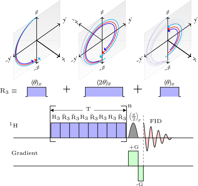
Figure 1: Refocusing protocol to minimize the effect of drive-inhomogeneity: Schematic representation of the refocusing scheme and the pulse sequence used in the experiment. $\text{R}_{3}$ is equivalent to an on-resonance $3$-pulse block composed of $\theta,2\theta,\theta$ pulses along $\hat{x},-\hat{x},\hat{x}$ respectively with $\theta\sim\pi$. $\bar{x}$ in the figure denotes the drive applied along $-\hat{x}$. The 3D diagrams atop the pulses show how the refocusing happens irrespective of the actual value of the flip angle $\theta$ and hence $\omega_{1}$. The pulse sequence below shows the operations performed on the proton (¹H) and the gradient channels respectively. After a recycle delay of $10\,{\rm s}(>6T_{1})$, we employ a super-cycle of R₃ inspired by WALTZ-8 as the drive sequence shakeefrefre83 . $\bar{\kern 1.8pt\rm R}_{3}$ indicates all pulses in R₃ are applied along inverted axis. $\big{[}\hskip 2.84544pt\big{]}^{n}$ implies that the sequence within the brackets is repeated $n$ times consecutively and $T$ denotes the length of a super-cycle. For detection, we have applied a Gaussian selective pulse of flip angle $\sim\pi/2$ in the presence of the applied gradient $+\text{G}$ to facilitate slice selection using spatial encoding. Immediately after the slice selection, an opposite compensatory gradient $-\text{G}$ is used to minimize phase distortion during slice-selection pavuram16 . The Free Induction Decay (FID) has been recorded in the absence of any gradient. Magnetization, $M_{z}$ is measured from the FID as a function of $n$. From the $M_{z}$ versus $nT$ data we measure $R_{z}$ using least-square curve fit.

To experimentally detect decay terms proportional to $\omega_{1}^{2}$, we choose the singlet imine protons in a dilute (millimolar) solution of commercially procured N-(4^′-methoxybenzylidene)-4-n-butylaniline (MBBA) in deuterated dimethyl sulfoxide (DMSO-D₆) placed in a static magnetic field along $\hat{z}$, as our target spin system. The application of an on-resonance ($\Delta\omega\rightarrow 0$) drive along $\hat{x}$, is shown to result in a damped nutation in the $y-z$ plane (if $\omega_{1}>1/T_{1},1/T_{2}$), starting from $\hat{z}$, with a damping rate proportional to $\omega_{1}^{2}$ as illustrated in Fig.2.

VII Results and Discussions

The $R_{z}$ versus $\omega_{1}$ data is fit with a parabola of the form $y=a_{1}+b_{1}x^{2}$ as shown in Fig. 2. From the fit we obtain the value of $\tau_{c}$ to be $1.32\times 10^{-11}\,$s. The value of $a_{1}$ is found to be $0.99\,$Hz which is same as the value of $(T_{1}+T_{2})/2T_{1}T_{2}$ within experimental error, the latter being estimated using standard measurement techniques furo81 ; cp54 ; mg58 . For the $R_{z}$ versus $\omega_{1}^{2}$ behavior, we find fair agreement between the theoretical prediction and the experimental observation. Hence we infer that our experimental results confirm the existence of the absorptive counter part of the Bloch-Siegert terms as predicted by our master equation (10).

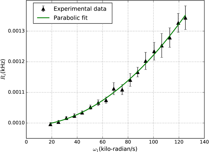
Figure 2: Experimentally observed damping of nutation due to drive: Plot of the decay rate $R_{z}$ versus the drive strength $\omega_{1}$. The upright triangles denote the experimentally determined values of $R_{z}$ with the vertical bars denoting the errors in the determination of $R_{z}$ at 95$\%$ level of confidence. The solid line (color online) shows the parabolic fit of the experimental data. Since the traditional Bloch Equations, predict $R_{z}$ to be independent of $\omega_{1}$, the above result unequivocally verifies the existence of the additional decay term originating from the absorptive part of the second order drive perturbation.

In all the experiments we calibrate our pulses using the fact that a $1.3$db pulse produces a nutation frequency of $14.25$kHz. The success of the refocusing scheme also relies on minimal translational diffusion during $\rm{R}_{3}$ which we presume to be the case since the duration of $\rm{R}_{3}$ is of the order of tens of $\mu$s. The maximum drive strength used in our experiments is $\omega_{1}/2\pi=20$kHz (close to the maximum permissible power) whereas the proton Larmor frequency of the spectrometer is of about $500$MHz. Thus the perturbative expansion used in deriving our master equation is valid for all practical considerations.

It is also possible to estimate the second order drive contribution through a spin-locking experiment, provided the initial magnetization is perfectly aligned along $x$ direction. However, the presence of the drive inhomogeneity will invariably leave part of the magnetization non-aligned along $x$. These components will exhibit nutation in the $y-z$ plane and subsequent analysis would be complicated. However, the on-resonance refocussed nutation scheme does not suffer from the effects of the drive inhomogeneity.

Our equation, as discussed before, allows $\omega_{1}$ to be a function of time as long as the timescale of change of $\omega_{1}$ remains slow compared to that of the fluctuations, which is the case in all pulsed NMR experiments in liquids. While the pulses are usually separated by sub-$\mu\!\text{s}$ rise-times and the tails, the timescales (of changes in the pulse envelopes) are several orders of magnitude larger than $\tau_{c}$, thereby the application of this formalism to pulsed NMR is completely within the assumed theoretical limits.

If a resonant drive is applied with $\Delta\omega\approx 0$, the evolution of the magnetization remains approximately confined to the $y-z$ plane. The departure from the $y-z$ plane i.e. the non-fulfillment of the resonant condition, occurs mostly due to incorrect shim conditions (static field inhomogeneity). Under a well-shimmed condition, $\Delta\omega\lesssim 1\text{Hz}$, and drive strengths $\omega_{1}\geq 1\text{kHz}$ – conditions which we satisfy in our experiments – the angle of the effective nutation axis is $\tan(\Delta\omega/\omega_{1})\sim 10^{-3}\sim 0$ (w.r.t. $x$ axis) for all practical purposes. Therefore, as long as the motion is effectively confined to the $y-z$ plane, change in the pulse phase by a value of $\pi$, would only result in a first order reversal of the motion of the magnetization while leaving the second order effects unchanged. The decay due to departure from the $y-z$ plain is expected to scale with the offset frequency $\Delta\omega$ and not with $\omega_{1}^{2}$ and as such cannot be used to explain our experimental findings.

VIII Conclusion

Our results reveal that the finite memory of the bath plays a central role in giving rise to time-nonlocal second-order complex susceptibility terms, having both dispersive and absorptive parts, from the external drive applied to the system. While the imaginary part of the susceptibility manifests itself as a dispersive shift term in the dynamics, its corresponding absorptive part provides a damping in addition to usual relaxation terms. The shift term due to resonant part of the drive is negligible, but the same due to the non-resonant part of the drive appears as the Bloch-Siegert shift under an asymptotic limit. The correction terms from the drive are extremely small yet measurable under suitable conditions, in the context of the solution-state NMR spectroscopy. For solid-state spectroscopy, such terms may not be negligible and provides a natural explanation for saturation processes. At extreme motional narrowing limit ($\tau_{c}\rightarrow 0$), the equation (10) predicts the expected unitary evolution of the system due to the drive, in the form of pure nutation. Our choice of $\delta$-correlated fluctuations lead to an exponential memory function; although other noise models may also serve the purpose. Since $\omega_{1}^{2}\tau_{c}\ll 1$, this damping decreases for smaller $\tau_{c}$ and hence it is envisaged that a bath with stronger fluctuations (towards the extreme motional narrowing limit) would make the system more immune to drive-induced damping and the shifts, which may have important consequences for ensemble quantum computing.

IX Acknowledgments

We acknowledge IISER Kolkata for providing the necessary funding and for providing access to the central NMR facility. A.C. would like to thank Anirban Mukherjee for insightful discussions and Centre for Scientific and Industrial Research (CSIR) India, for a senior research fellowship.

Appendix A Construction of the finite propagator

Following the description of the system and the lattice laid out in the main manuscript and the notations introduced therein, we intend to construct a finite propagator $U(t_{1})$, valid for the coarse-grained time interval, $t_{1}\in[t,t+\Delta t]$. The coarse-graining time $\Delta t$ is such that the contribution of $H_{\scriptscriptstyle\rm eff}$ in $U(t_{1})$ can be linearized and only the leading first order terms are retained. On the contrary, many instances of the fluctuation take place within $\Delta t$ and as such we retain all possible higher order terms of $H_{\scriptscriptstyle\rm L}$. The explicit construction of the finite-time propagator begins from the Schrödinger equation:

$$\frac{d}{dt}U(t)=-i\,H(t)\,U(t)$$ (17)

and its formal solution in the domain $[t,t_{1}]$ (with $t_{1}>t$):

$$U(t_{1}) = \mathbbm{1}-i\,\int\limits_{t}^{t_{1}}dt_{2}\,H(t_{2})\,U(t_{2})$$ (18)

$$= \mathbbm{1}-i\,\int\limits_{t}^{t_{1}}dt_{2}\,H_{\scriptscriptstyle\rm eff}(t_{2})\,U(t_{2})-i\,\int\limits_{t}^{t_{1}}dt_{2}\,H_{\scriptscriptstyle\rm L}(t_{2})\,U(t_{2}).$$

Since $t_{1}\in[t,t+\Delta t]$ by assumption, the interval $(t_{1}-t)\ll 1/\omega_{1},1/\omega_{\scriptscriptstyle\rm SL}$ and as such further propagation due to $H_{\scriptscriptstyle\rm eff}$ can be neglected on the r.h.s of equation (18). Thus collecting all the remaining terms in the r.h.s. of equation (18) we get a finite propagator with a leading linear order term in $H_{\scriptscriptstyle\rm eff}$ of the form

$$U(t_{1})\approx\mathbbm{1}-i\,\int\limits_{t}^{t_{1}}dt_{2}\,H_{\scriptscriptstyle\rm eff}(t_{2})\,U_{\scriptscriptstyle\rm L}(t_{2})-i\,\int\limits_{t}^{t_{1}}dt_{2}\,H_{\scriptscriptstyle\rm L}(t_{2})\,U_{\scriptscriptstyle\rm L}(t_{2}).$$ (19)

Combining the last term in the r.h.s. with the identity we can rewrite the above equation as,

$$U(t_{1})\approx U_{\scriptscriptstyle\rm L}(t_{1})-i\,\int\limits_{t}^{t_{1}}dt_{2}\,H_{\scriptscriptstyle\rm eff}(t_{2})\,U_{\scriptscriptstyle\rm L}(t_{2}).$$ (20)

Appendix B Emergence of the memory of the bath from the fluctuations

Following the usual practice, we too assume that at the beginning of the coarse-graining interval the full density matrix has the factorized form

$$\rho(t)=\rho_{\scriptscriptstyle\rm S}(t)\otimes\rho_{\scriptscriptstyle\rm L}^{\scriptscriptstyle\rm eq},$$ (21)

where $\rho(t)=\overline{\widetilde{\rho}(t)}$ and $\rho_{\scriptscriptstyle\rm L}^{\scriptscriptstyle\rm eq}=\text{exp}(-\beta\mathcal{H}_{\scriptscriptstyle\rm L}^{\circ})/\mathcal{Z}_{\scriptscriptstyle\rm L}$ denotes the equilibrium density matrix of the lattice cotandurogryn04 ; wangblo53 ; brepet02 .

We thus have,

$$\overline{U_{\scriptscriptstyle\rm L}(t_{1})\widetilde{\rho}(t)U_{\scriptscriptstyle\rm L}^{\dagger}(t_{2})}=\rho_{S}(t)\otimes\sum_{j}\frac{e^{-\beta\omega_{j}}}{\mathcal{Z}_{L}}|\phi_{j}\rangle\langle\phi_{j}|\overline{\exp\big{\{}-i\int_{t}^{t_{1}}dt_{3}\,f_{j}(t_{3})+i\int_{t}^{t_{2}}dt_{4}\,f_{j}(t_{4})\big{\}}}.$$ (22)

In the above expression $\omega_{j}$ denotes the eigen-value of $\mathcal{H}_{\scriptscriptstyle\rm L}^{\circ}$ corresponding to $|\phi_{j}\rangle$ and we have made use of the fact that $H_{\scriptscriptstyle\rm L}(t)$ and thus the propagators $U_{\scriptscriptstyle\rm L}(t_{1})$ are independent of the initial distribution of the lattice states $\forall t_{1}\geq t$.

Thus we obtain,

$$\overline{U_{\scriptscriptstyle\rm L}(t_{1})\widetilde{\rho}(t)U_{\scriptscriptstyle\rm L}^{\dagger}(t_{2})}=\rho_{\scriptscriptstyle\rm S}(t)\otimes\rho_{\scriptscriptstyle\rm L}^{\scriptscriptstyle\rm eq}\exp\big{(}-\frac{1}{2}\kappa^{2}|t_{1}-t_{2}|\big{)}.\\$$ (23)

In deriving the above, we have used the cumulant expansion for Gaussian stochastic processes with usual $\delta$-correlation in time, for which only the terms upto the second cumulant survive. A further assumption of zero mean (as in our model) leaves only the exponentially decaying factor, $\exp\big{(}-\frac{1}{2}\kappa^{2}|t_{1}-t_{2}|\big{)}$.

Appendix C Explicit derivation of the drive-contributions in the Bloch Equations

The measured magnetization components for the spin-$1/2$ ensemble are given by $M_{\alpha}(t)=\text{Tr}_{\scriptscriptstyle\rm S}[F_{\scriptscriptstyle\rm\alpha}^{\scriptscriptstyle\rm R}(t)\rho_{\scriptscriptstyle\rm S}(t)]$, $\alpha\in\{x,y,z\}$. Thus, using the master equation derived in the main manuscript and the observables defined using equations (11) in the manuscript, we obtain,

$$\frac{d}{dt}M_{\scriptscriptstyle\rm\alpha}(t) = \text{Tr}_{\scriptscriptstyle\rm S}\Big{[}\Big{\{}\frac{d}{dt}F_{\scriptscriptstyle\rm\alpha}^{\scriptscriptstyle\rm R}(t)\Big{\}}\rho_{\scriptscriptstyle\rm S}(t)\Big{]}+\text{Tr}_{\scriptscriptstyle\rm S}\Big{[}F_{\scriptscriptstyle\rm\alpha}^{\scriptscriptstyle\rm R}(t)\Big{\{}\frac{d}{dt}\rho_{\scriptscriptstyle\rm S}(t)\Big{\}}\Big{]}$$ (24)

$$= \text{Tr}_{\scriptscriptstyle\rm S}\Big{[}\Big{\{}\frac{d}{dt}F_{\scriptscriptstyle\rm\alpha}^{\scriptscriptstyle\rm R}(t)\Big{\}}\rho_{\scriptscriptstyle\rm S}(t)\Big{]}-i\,\text{Tr}_{\scriptscriptstyle\rm S}\Big{\{}{\rm Tr}_{\scriptscriptstyle\rm L}\!\left[H_{\scriptscriptstyle\rm eff}(t),\,\rho_{\scriptscriptstyle\rm S}(t)\otimes\rho_{\scriptscriptstyle\rm L}^{\scriptscriptstyle\rm eq}\right]^{\scriptscriptstyle\rm sec}F_{\scriptscriptstyle\rm\alpha}^{\scriptscriptstyle\rm R}(t)\Big{\}}$$

$$-\int\limits_{0}^{\infty}\kern-2.0ptd\tau\;\text{Tr}_{\scriptscriptstyle\rm S}\Big{\{}{\rm Tr}_{\scriptscriptstyle\rm L}\!\left[H_{\scriptscriptstyle\rm eff}(t),\,\left[H_{\scriptscriptstyle\rm eff}(t-\tau),\rho_{\scriptscriptstyle\rm S}(t)\otimes\rho_{\scriptscriptstyle\rm L}^{\scriptscriptstyle\rm eq}\right]\right]^{\scriptscriptstyle\rm sec}e^{-{|\tau|}/{\tau_{c}}}F_{\scriptscriptstyle\rm\alpha}^{\scriptscriptstyle\rm R}(t)\Big{\}}.$$

The first term in the r.h.s. of the last equation above is easy to evaluate. For the dynamical equation for $M_{\scriptscriptstyle\rm y}(t)$, this term becomes

$$\text{Tr}_{\scriptscriptstyle\rm S}\Big{[}\Big{\{}\frac{d}{dt}F_{\scriptscriptstyle\rm y}^{\scriptscriptstyle\rm R}(t)\Big{\}}\rho_{\scriptscriptstyle\rm S}(t)\Big{]} = \text{Tr}_{\scriptscriptstyle\rm S}\Big{[}\frac{1}{2i}\frac{d}{dt}\big{\{}I_{+}e^{-i\Delta\omega t}-I_{-}e^{i\Delta\omega t}\big{\}}\rho_{\scriptscriptstyle\rm S}(t)\Big{]}$$ (25)

$$= -\Delta\omega\text{Tr}_{\scriptscriptstyle\rm S}\Big{[}\frac{1}{2}\big{\{}I_{+}e^{-i\Delta\omega t}+I_{-}e^{i\Delta\omega t}\big{\}}\rho_{\scriptscriptstyle\rm S}(t)\Big{]}$$

$$= -\Delta\omega\,M_{\scriptscriptstyle\rm x}(t).$$

Similarly, for the other magnetization components we have from the first term in the r.h.s of equation (24),

$$\text{Tr}_{\scriptscriptstyle\rm S}\Big{[}\Big{\{}\frac{d}{dt}F_{\scriptscriptstyle\rm z}^{\scriptscriptstyle\rm R}(t)\Big{\}}\rho_{\scriptscriptstyle\rm S}(t)\Big{]}=0$$ (26)

and

$$\text{Tr}_{\scriptscriptstyle\rm S}\Big{[}\Big{\{}\frac{d}{dt}F_{\scriptscriptstyle\rm x}^{\scriptscriptstyle\rm R}(t)\Big{\}}\rho_{\scriptscriptstyle\rm S}(t)\Big{]}=\Delta\omega\,M_{\scriptscriptstyle\rm y}(t).$$ (27)

C.1 First order drive contribution

The condition $\text{Tr}_{\scriptscriptstyle\rm L}[H_{\scriptscriptstyle\rm SL}(t),\rho_{\scriptscriptstyle\rm S}(t)\otimes\rho_{\scriptscriptstyle\rm L}^{\scriptscriptstyle\rm eq}]=0$ ensures that only the external drive, $H_{\scriptscriptstyle\rm S}(t)$ contributes in the second term on the r.h.s. of equation (24). Of this only the secular terms (co-rotating terms i.e. terms with frequency $\Delta\omega$ in the interaction representation) are non-negligible. Thus we have

$$-i\,\text{Tr}_{\scriptscriptstyle\rm S}\Big{\{}{\rm Tr}_{\scriptscriptstyle\rm L}\!\left[H_{\scriptscriptstyle\rm S}(t),\,\rho_{\scriptscriptstyle\rm S}(t)\otimes\rho_{\scriptscriptstyle\rm L}^{\scriptscriptstyle\rm eq}\right]^{\scriptscriptstyle\rm sec}F_{\scriptscriptstyle\rm\alpha}^{\scriptscriptstyle\rm R}(t)\Big{\}} = -i\,\text{Tr}_{\scriptscriptstyle\rm S}\Big{\{}\omega_{1}{\rm Tr}_{\scriptscriptstyle\rm L}\!\left[F_{\scriptscriptstyle\rm x}^{\scriptscriptstyle\rm C}(t)+F_{\scriptscriptstyle\rm x}^{\scriptscriptstyle\rm R}(t),\,\rho_{\scriptscriptstyle\rm S}(t)\otimes\rho_{\scriptscriptstyle\rm L}^{\scriptscriptstyle\rm eq}\right]^{\scriptscriptstyle\rm sec}F_{\scriptscriptstyle\rm\alpha}^{\scriptscriptstyle\rm R}(t)\Big{\}}$$ (28)

$$= -i\,\text{Tr}_{\scriptscriptstyle\rm S}\Big{\{}\omega_{1}\!\left[F_{\scriptscriptstyle\rm x}^{\scriptscriptstyle\rm C}(t)+F_{\scriptscriptstyle\rm x}^{\scriptscriptstyle\rm R}(t),\,\rho_{\scriptscriptstyle\rm S}(t)\right]^{\scriptscriptstyle\rm sec}F_{\scriptscriptstyle\rm\alpha}^{\scriptscriptstyle\rm R}(t)\Big{\}}$$

$$= -i\,\text{Tr}_{\scriptscriptstyle\rm S}\Big{\{}\omega_{1}\!\left[F_{\scriptscriptstyle\rm x}^{\scriptscriptstyle\rm R}(t),\,\rho_{\scriptscriptstyle\rm S}(t)\right]F_{\scriptscriptstyle\rm\alpha}^{\scriptscriptstyle\rm R}(t)\Big{\}}$$

$$= -i\,\text{Tr}_{\scriptscriptstyle\rm S}\Big{\{}\omega_{1}\!\left[F_{\scriptscriptstyle\rm\alpha}^{\scriptscriptstyle\rm R}(t),\,F_{\scriptscriptstyle\rm x}^{\scriptscriptstyle\rm R}(t)\right]\rho_{\scriptscriptstyle\rm S}(t)\Big{\}},$$

where in the second-last step we have removed the non-secular counter-rotating term, $F_{\scriptscriptstyle\rm x}^{\scriptscriptstyle\rm C}(t)$ and hence the superscript ‘sec’ is dropped thereafter. In the above derivation we have used the fact that ${\rm Tr}_{\scriptscriptstyle\rm L}[\rho_{L}^{\rm eq}]=1$. For evaluating the commutators of $F_{\scriptscriptstyle\rm\alpha}^{\scriptscriptstyle\rm R}(t)$ we note that

$$\Big{[}F_{\scriptscriptstyle\rm\alpha_{k}}^{\scriptscriptstyle\rm R}(t),F_{\scriptscriptstyle\rm\alpha_{m}}^{\scriptscriptstyle\rm R}(t)\Big{]} = \Big{[}e^{-i\Delta\omega tI_{z}}I_{\scriptscriptstyle\rm\alpha_{k}}e^{i\Delta\omega tI_{z}},e^{-i\Delta\omega tI_{z}}I_{\scriptscriptstyle\rm\alpha_{m}}e^{i\Delta\omega tI_{z}}\Big{]}$$ (29)

$$= e^{-i\Delta\omega tI_{z}}\Big{[}I_{\scriptscriptstyle\rm\alpha_{k}},I_{\scriptscriptstyle\rm\alpha_{m}}\Big{]}e^{i\Delta\omega tI_{z}}$$

$$= i\,\varepsilon_{pkm}\,e^{-i\Delta\omega tI_{z}}I_{\scriptscriptstyle\rm\alpha_{p}}e^{i\Delta\omega tI_{z}}$$

$$= i\,\varepsilon_{pkm}\,F_{\scriptscriptstyle\rm\alpha_{p}}^{\scriptscriptstyle\rm R}(t),$$

where, $\{k,m,p\}\in\{1,2,3\}$, $\alpha_{1}=x$, $\alpha_{2}=y$ and $\alpha_{3}=z$ and $\varepsilon_{pkm}$ is the Levi-Civita symbol. Substituting the expression for $F_{\scriptscriptstyle\rm\alpha}^{\scriptscriptstyle\rm R}$ in the last line of the above expression one can readily find the first-order drive contribution in the dynamics of $M_{\scriptscriptstyle\rm\alpha}(t)$. For example, in the dynamics of $M_{\scriptscriptstyle\rm y}(t)$, we have

$$-i\,\text{Tr}_{\scriptscriptstyle\rm S}\Big{\{}{\rm Tr}_{\scriptscriptstyle\rm L}\!\left[H_{\scriptscriptstyle\rm S}(t),\,\rho_{\scriptscriptstyle\rm S}(t)\otimes\rho_{\scriptscriptstyle\rm L}^{\scriptscriptstyle\rm eq}\right]^{\scriptscriptstyle\rm sec}F_{\scriptscriptstyle\rm y}^{\scriptscriptstyle\rm R}(t)\Big{\}} = -i\,\text{Tr}_{\scriptscriptstyle\rm S}\Big{\{}\omega_{1}\!\left[F_{\scriptscriptstyle\rm y}^{\scriptscriptstyle\rm R}(t),\,F_{\scriptscriptstyle\rm x}^{\scriptscriptstyle\rm R}(t)\right]\rho_{\scriptscriptstyle\rm S}(t)\Big{\}}$$ (30)

$$= -i\,\text{Tr}_{\scriptscriptstyle\rm S}\Big{\{}\omega_{1}\!(-i)F_{\scriptscriptstyle\rm z}^{\scriptscriptstyle\rm R}\rho_{\scriptscriptstyle\rm S}(t)\Big{\}}$$

$$= -\omega_{1}\,M_{\scriptscriptstyle\rm z}(t).$$

C.2 Second order drive contribution

In the third expression on the r.h.s. of equation (24), the cross-terms between $H_{\scriptscriptstyle\rm SL}(t)$ and $H_{\scriptscriptstyle\rm S}(t)$ vanish due to the condition $\text{Tr}_{\scriptscriptstyle\rm L}[H_{\scriptscriptstyle\rm SL}(t),\rho_{\scriptscriptstyle\rm S}(t)\otimes\rho_{\scriptscriptstyle\rm L}^{\scriptscriptstyle\rm eq}]=0$. Only contributions in this expression comes from the self-terms of $H_{\scriptscriptstyle\rm SL}(t)$ and $H_{\scriptscriptstyle\rm S}(t)$. We assume a generic form of the coupling Hamiltonian for the spin-$\frac{1}{2}$ ensemble, following Wangsness and Bloch, which leads to the relaxation terms proportional to $1/T_{1}$ and $1/T_{2}$ with the equilibrium magnetization $M_{\circ}$ as shown in their work (Lamb-shift terms being neglected) wangblo53 . Since the calculations involved follow exactly that of Bloch and Wangsness and is not the main focus of this work, we shall assume the existence of these relaxation terms in our equations of motion without elaborating further. The second-order drive contribution is given by

$$-\int\limits_{0}^{\infty}\kern-2.0ptd\tau\;\text{Tr}_{\scriptscriptstyle\rm S}\Big{\{}{\rm Tr}_{\scriptscriptstyle\rm L}\!\big{[}H_{\scriptscriptstyle\rm S}(t),\,\big{[}H_{\scriptscriptstyle\rm S}(t-\tau),\rho_{\scriptscriptstyle\rm S}(t)\otimes\rho_{\scriptscriptstyle\rm L}^{\scriptscriptstyle\rm eq}\big{]}\big{]}^{\scriptscriptstyle\rm sec}e^{-{|\tau|}/{\tau_{c}}}F_{\scriptscriptstyle\rm\alpha}^{\scriptscriptstyle\rm R}(t)\Big{\}}$$

$$=-\omega_{1}^{2}\int\limits_{0}^{\infty}\kern-2.0ptd\tau\;\text{Tr}_{\scriptscriptstyle\rm S}\Big{\{}\big{[}F_{\scriptscriptstyle\rm x}^{\scriptscriptstyle\rm C}(t)+F_{\scriptscriptstyle\rm x}^{\scriptscriptstyle\rm R}(t),\,\big{[}F_{\scriptscriptstyle\rm x}^{\scriptscriptstyle\rm C}(t-\tau)+F_{\scriptscriptstyle\rm x}^{\scriptscriptstyle\rm R}(t-\tau),\rho_{\scriptscriptstyle\rm S}(t)\big{]}\big{]}^{\scriptscriptstyle\rm sec}e^{-{|\tau|}/{\tau_{c}}}F_{\scriptscriptstyle\rm\alpha}^{\scriptscriptstyle\rm R}(t)\Big{\}}$$

$$=-\frac{1}{4}\omega_{1}^{2}\int\limits_{0}^{\infty}\kern-2.0ptd\tau\;\text{Tr}_{\scriptscriptstyle\rm S}\Big{\{}\big{[}\big{(}I_{+}e^{i\Omega t}+I_{-}e^{-i\Omega t}\big{)}+\big{(}I_{+}e^{-i\Delta\omega t}+I_{-}e^{i\Delta\omega t}\big{)},$$

$$\hskip 56.9055pt\big{[}\big{(}I_{+}e^{i\Omega(t-\tau)}+I_{-}e^{-i\Omega(t-\tau)}\big{)}+\big{(}I_{+}e^{-i\Delta\omega(t-\tau)}+I_{-}e^{i\Delta\omega(t-\tau)}\big{)},\rho_{\scriptscriptstyle\rm S}(t)\big{]}\big{]}^{\scriptscriptstyle\rm sec}F_{\scriptscriptstyle\rm\alpha}^{\scriptscriptstyle\rm R}(t)\Big{\}}e^{-{|\tau|}/{\tau_{c}}},$$ (31)

where we have again used the fact that ${\rm Tr}_{\scriptscriptstyle\rm L}[\rho_{L}^{\rm eq}]=1$.

To determine secular terms in the above expression we follow the analysis prescribed by Cohen-Tannoudji et. al cotandurogryn04 . We note that the terms oscillating with $\Delta\omega$ are not averaged out during the interval $\Delta t$. Thus the secular approximation retains the full self-term of $F_{\scriptscriptstyle\rm x}^{\scriptscriptstyle\rm R}(t)$ in the second-order of the drive. On the other hand all cross-terms between $F_{\scriptscriptstyle\rm x}^{\scriptscriptstyle\rm C}(t)$ and $F_{\scriptscriptstyle\rm x}^{\scriptscriptstyle\rm R}(t)$ become negligible in the secular limit. In the self-terms of $F_{\scriptscriptstyle\rm x}^{\scriptscriptstyle\rm C}(t)$, only the cross-commutators between $I_{+}$ and $I_{-}$ survive the secular integration. Thus we finally arrive at the following form of the secular second-order drive contributions:

$$-\int\limits_{0}^{\infty}\kern-2.0ptd\tau\;\text{Tr}_{\scriptscriptstyle\rm S}\Big{\{}{\rm Tr}_{\scriptscriptstyle\rm L}\!\big{[}H_{\scriptscriptstyle\rm S}(t),\,\big{[}H_{\scriptscriptstyle\rm S}(t-\tau),\rho_{\scriptscriptstyle\rm S}(t)\otimes\rho_{\scriptscriptstyle\rm L}^{\scriptscriptstyle\rm eq}\big{]}\big{]}^{\scriptscriptstyle\rm sec}e^{-{|\tau|}/{\tau_{c}}}F_{\scriptscriptstyle\rm\alpha}^{\scriptscriptstyle\rm R}(t)\Big{\}}$$

$$=-\frac{1}{4}\omega_{1}^{2}\int\limits_{0}^{\infty}\kern-2.0ptd\tau\;\text{Tr}_{\scriptscriptstyle\rm S}\Big{\{}\big{[}I_{+}e^{i\Omega t},\big{[}I_{-}e^{-i\Omega(t-\tau)},\rho_{\scriptscriptstyle\rm S}(t)\big{]}\big{]}F_{\scriptscriptstyle\rm\alpha}^{\scriptscriptstyle\rm R}(t)+\big{[}I_{-}e^{-i\Omega t},\big{[}I_{+}e^{i\Omega(t-\tau)},\rho_{\scriptscriptstyle\rm S}(t)\big{]}\big{]}F_{\scriptscriptstyle\rm\alpha}^{\scriptscriptstyle\rm R}(t)$$

$$\hskip 56.9055pt+\big{[}\big{(}I_{+}e^{-i\Delta\omega t}+I_{-}e^{i\Delta\omega t}\big{)},\big{[}\big{(}I_{+}e^{-i\Delta\omega(t-\tau)}+I_{-}e^{i\Delta\omega(t-\tau)}\big{)},\rho_{\scriptscriptstyle\rm S}(t)\big{]}\big{]}F_{\scriptscriptstyle\rm\alpha}^{\scriptscriptstyle\rm R}(t)\Big{\}}e^{-{|\tau|}/{\tau_{c}}}$$

$$=-\frac{1}{4}\omega_{1}^{2}\Big{[}\int\limits_{0}^{\infty}\kern-2.0ptd\tau\,e^{i\Omega\tau}e^{-{|\tau|}/{\tau_{c}}}\Big{]}\;\text{Tr}_{\scriptscriptstyle\rm S}\Big{\{}\big{[}I_{-},\big{[}I_{+},F_{\scriptscriptstyle\rm\alpha}^{\scriptscriptstyle\rm R}(t)\big{]}\big{]}\rho_{\scriptscriptstyle\rm S}(t)\Big{\}}-\frac{1}{4}\omega_{1}^{2}\Big{[}\int\limits_{0}^{\infty}\kern-2.0ptd\tau\,e^{-i\Omega\tau}e^{-{|\tau|}/{\tau_{c}}}\Big{]}\;\text{Tr}_{\scriptscriptstyle\rm S}\Big{\{}\big{[}I_{+},\big{[}I_{-},F_{\scriptscriptstyle\rm\alpha}^{\scriptscriptstyle\rm R}(t)\big{]}\big{]}\rho_{\scriptscriptstyle\rm S}(t)\Big{\}}$$

$$\hskip 14.22636pt-\omega_{1}^{2}\int\limits_{0}^{\infty}\kern-2.0ptd\tau\;\text{Tr}_{\scriptscriptstyle\rm S}\Big{\{}\big{[}F_{\scriptscriptstyle\rm x}^{\scriptscriptstyle\rm R}(t-\tau),\big{[}F_{\scriptscriptstyle\rm x}^{\scriptscriptstyle\rm R}(t),F_{\scriptscriptstyle\rm\alpha}^{\scriptscriptstyle\rm R}(t)\big{]}\big{]}\rho_{\scriptscriptstyle\rm S}(t)\Big{\}}e^{-{|\tau|}/{\tau_{c}}}$$

$$=-\frac{1}{4}\omega_{1}^{2}\Gamma(\Omega)\text{Tr}_{\scriptscriptstyle\rm S}\Big{\{}\big{[}I_{-},\big{[}I_{+},F_{\scriptscriptstyle\rm\alpha}^{\scriptscriptstyle\rm R}(t)\big{]}\big{]}\rho_{\scriptscriptstyle\rm S}(t)\Big{\}}-\frac{1}{4}\omega_{1}^{2}\Gamma^{*}(\Omega)\text{Tr}_{\scriptscriptstyle\rm S}\Big{\{}\big{[}I_{+},\big{[}I_{-},F_{\scriptscriptstyle\rm\alpha}^{\scriptscriptstyle\rm R}(t)\big{]}\big{]}\rho_{\scriptscriptstyle\rm S}(t)\Big{\}}$$

$$\hskip 14.22636pt-\omega_{1}^{2}\int\limits_{0}^{\infty}\kern-2.0ptd\tau\;\text{Tr}_{\scriptscriptstyle\rm S}\Big{\{}\big{[}F_{\scriptscriptstyle\rm x}^{\scriptscriptstyle\rm R}(t-\tau),\big{[}F_{\scriptscriptstyle\rm x}^{\scriptscriptstyle\rm R}(t),F_{\scriptscriptstyle\rm\alpha}^{\scriptscriptstyle\rm R}(t)\big{]}\big{]}\rho_{\scriptscriptstyle\rm S}(t)\Big{\}}e^{-{|\tau|}/{\tau_{c}}},$$ (32)

where $\Gamma(\Omega)=\Big{[}\int\limits_{0}^{\infty}\kern-2.0ptd\tau\,e^{i\Omega\tau}e^{-{|\tau|}/{\tau_{c}}}\Big{]}$ and hence its complex conjugate, $\Gamma^{*}(\Omega)=\Big{[}\int\limits_{0}^{\infty}\kern-2.0ptd\tau\,e^{-i\Omega\tau}e^{-{|\tau|}/{\tau_{c}}}\Big{]}$. $\Gamma(\Omega)$ is a complex Lorentzian centered at $\Omega$ having real and imaginary parts given by

$$\Gamma(\Omega)=\frac{\tau_{c}}{1+\Omega^{2}\tau_{c}^{2}}+i\frac{\Omega\tau_{c}^{2}}{1+\Omega^{2}\tau_{c}^{2}},$$ (33)

which are Kramers-Kronig pairs. Substituting the expression for $F_{\scriptscriptstyle\rm\alpha}^{\scriptscriptstyle\rm R}$ in the last line of the equation (C.2) we find the full second-order drive contribution in the dynamics of $M_{\scriptscriptstyle\rm\alpha}(t)$. Again as an example, the second-order contribution of the drive in the dynamical equation of $M_{\scriptscriptstyle\rm y}(t)$ is obtained after substituting $F_{\scriptscriptstyle\rm y}^{\scriptscriptstyle\rm R}$ in place of $F_{\scriptscriptstyle\rm\alpha}^{\scriptscriptstyle\rm R}$ and is given by:

$$-\frac{1}{4}\omega_{1}^{2}\Gamma^{*}(\Omega)\text{Tr}_{\scriptscriptstyle\rm S}\Big{\{}\frac{1}{2i}\big{[}I_{+},\big{[}I_{-},I_{+}\big{]}\big{]}\,e^{-i\Delta\omega t}\rho_{\scriptscriptstyle\rm S}(t)\Big{\}}-\frac{1}{4}\omega_{1}^{2}\Gamma(\Omega)\text{Tr}_{\scriptscriptstyle\rm S}\Big{\{}-\frac{1}{2i}\big{[}I_{-},\big{[}I_{+},I_{-}\big{]}\big{]}\,e^{i\Delta\omega t}\rho_{\scriptscriptstyle\rm S}(t)\Big{\}}$$

$$\hskip 14.22636pt-\omega_{1}^{2}\int\limits_{0}^{\infty}\kern-2.0ptd\tau\;\text{Tr}_{\scriptscriptstyle\rm S}\Big{\{}i\big{[}\big{(}I_{+}e^{-i\Delta\omega(t-\tau)}+I_{-}e^{i\Delta\omega(t-\tau)}\big{)},I_{z}\big{]}\rho_{\scriptscriptstyle\rm S}(t)\Big{\}}e^{-{|\tau|}/{\tau_{c}}}$$

$$=-\frac{1}{4i}\omega_{1}^{2}\Big{[}\frac{\tau_{c}}{1+\Omega^{2}\tau_{c}^{2}}-i\frac{\Omega\tau_{c}^{2}}{1+\Omega^{2}\tau_{c}^{2}}\Big{]}\text{Tr}_{\scriptscriptstyle\rm S}[I_{+}e^{-i\Delta\omega t}\rho_{\scriptscriptstyle\rm S}(t)]+\frac{1}{4i}\omega_{1}^{2}\Big{[}\frac{\tau_{c}}{1+\Omega^{2}\tau_{c}^{2}}+i\frac{\Omega\tau_{c}^{2}}{1+\Omega^{2}\tau_{c}^{2}}\Big{]}\text{Tr}_{\scriptscriptstyle\rm S}[I_{-}e^{i\Delta\omega t}\rho_{\scriptscriptstyle\rm S}(t)\big{]}$$

$$\hskip 14.22636pt-\frac{1}{2i}\omega_{1}^{2}\Big{[}\frac{\tau_{c}}{1+\Delta\omega^{2}\tau_{c}^{2}}-i\frac{\Delta\omega\tau_{c}^{2}}{1+\Delta\omega^{2}\tau_{c}^{2}}\Big{]}\text{Tr}_{\scriptscriptstyle\rm S}[I_{+}e^{-i\Delta\omega t}\rho_{\scriptscriptstyle\rm S}(t)]+\frac{1}{2i}\omega_{1}^{2}\Big{[}\frac{\tau_{c}}{1+\Delta\omega^{2}\tau_{c}^{2}}+i\frac{\Delta\omega\tau_{c}^{2}}{1+\Delta\omega^{2}\tau_{c}^{2}}\Big{]}\text{Tr}_{\scriptscriptstyle\rm S}[I_{-}e^{i\Delta\omega t}\rho_{\scriptscriptstyle\rm S}(t)\big{]}.$$ (34)

Simplifying the above expression we have,

$$-\frac{1}{2}\omega_{1}^{2}\Big{[}\frac{\tau_{c}}{1+\Omega^{2}\tau_{c}^{2}}\Big{]}\text{Tr}_{\scriptscriptstyle\rm S}\big{[}\frac{1}{2i}\big{(}I_{+}e^{-i\Delta\omega t}-I_{-}e^{i\Delta\omega t}\big{)}\rho_{\scriptscriptstyle\rm S}(t)\big{]}-\omega_{1}^{2}\Big{[}\frac{\tau_{c}}{1+\Delta\omega^{2}\tau_{c}^{2}}\Big{]}\text{Tr}_{\scriptscriptstyle\rm S}\big{[}\frac{1}{2i}\big{(}I_{+}e^{-i\Delta\omega t}-I_{-}e^{i\Delta\omega t}\big{)}\rho_{\scriptscriptstyle\rm S}(t)\big{]}$$

$$\hskip 5.69046pt+\frac{1}{2}\omega_{1}^{2}\Big{[}\frac{\Omega^{2}\tau_{c}^{2}}{1+\Omega^{2}\tau_{c}^{2}}\Big{]}\text{Tr}_{\scriptscriptstyle\rm S}\big{[}\frac{1}{2}\big{(}I_{+}e^{-i\Delta\omega t}+I_{-}e^{i\Delta\omega t}\big{)}\rho_{\scriptscriptstyle\rm S}(t)\big{]}+\omega_{1}^{2}\Big{[}\frac{\Delta\omega^{2}\tau_{c}^{2}}{1+\Delta\omega^{2}\tau_{c}^{2}}\Big{]}\text{Tr}_{\scriptscriptstyle\rm S}\big{[}\frac{1}{2}\big{(}I_{+}e^{-i\Delta\omega t}+I_{-}e^{i\Delta\omega t}\big{)}\rho_{\scriptscriptstyle\rm S}(t)\big{]}$$

$$=-\frac{1}{2}\omega_{1}^{2}\Big{[}\frac{\tau_{c}}{1+\Omega^{2}\tau_{c}^{2}}\Big{]}\text{Tr}_{\scriptscriptstyle\rm S}\big{[}F_{\scriptscriptstyle\rm y}^{\scriptscriptstyle\rm R}(t)\rho_{\scriptscriptstyle\rm S}(t)\big{]}-\omega_{1}^{2}\Big{[}\frac{\tau_{c}}{1+\Delta\omega^{2}\tau_{c}^{2}}\Big{]}\text{Tr}_{\scriptscriptstyle\rm S}\big{[}F_{\scriptscriptstyle\rm y}^{\scriptscriptstyle\rm R}(t)\rho_{\scriptscriptstyle\rm S}(t)\big{]}$$

$$\hskip 5.69046pt+\frac{1}{2}\omega_{1}^{2}\Big{[}\frac{\Omega^{2}\tau_{c}^{2}}{1+\Omega^{2}\tau_{c}^{2}}\Big{]}\text{Tr}_{\scriptscriptstyle\rm S}\big{[}F_{\scriptscriptstyle\rm x}^{\scriptscriptstyle\rm R}(t)\rho_{\scriptscriptstyle\rm S}(t)\big{]}+\omega_{1}^{2}\Big{[}\frac{\Delta\omega^{2}\tau_{c}^{2}}{1+\Delta\omega^{2}\tau_{c}^{2}}\Big{]}\text{Tr}_{\scriptscriptstyle\rm S}\big{[}F_{\scriptscriptstyle\rm x}^{\scriptscriptstyle\rm R}(t)\rho_{\scriptscriptstyle\rm S}(t)\big{]}$$

$$=-\eta_{y}M_{\scriptscriptstyle\rm y}(t)+(\omega_{\scriptscriptstyle\rm BS}+\delta\omega)M_{\scriptscriptstyle\rm x}(t),$$ (35)

where,

$$\omega_{\scriptscriptstyle\rm BS}=\frac{1}{2}\Big{(}\frac{\omega_{1}^{2}\Omega\tau_{c}^{2}}{1+\Omega^{2}\tau_{c}^{2}}\Big{)},$$ (36)

$$\delta\omega=\frac{\omega_{1}^{2}\Delta\omega\tau_{c}^{2}}{1+\Delta\omega^{2}\tau_{c}^{2}}$$ (37)

and

$$\eta_{y}=\omega_{1}^{2}\Big{[}\frac{1}{2}\Big{(}\frac{\tau_{c}}{1+\Omega^{2}\tau_{c}^{2}}\Big{)}+\frac{\tau_{c}}{1+\Delta\omega^{2}\tau_{c}^{2}}\Big{]}.$$ (38)

The second-order drive contributions in the dynamics of the other magnetization components follow in a similar way.

References

- (1) Wangsness R.K. & Bloch, F. The dynamical theory of nuclear induction. Phys. Rev. 89, 728–739 (1953).
- (2) Abragam, A. Principles Of Nuclear Magnetism (International Series Of Monographs On Physics). Clarendon Press, Oxford (1961).
- (3) Vega, A.J. & Vaughan, R.W. Nuclear spin–lattice relaxation in periodically irradiated systems. J. Chem. Phys. 68, 1958–1966 (1978).
- (4) Cohen-Tannoudji, C. Dupont-Roc, J. & Gilbert, G. Atom-Photon Interactions: Basic Processes And Applications. WILEY-VCH, Germany (2004).
- (5) Bloch, F. & Siegert A. Magnetic resonance for nonrotating fields. Phys. Rev. 57, 522–527 (1940).
- (6) Shirley, J.H. Solution of the Schrödinger equation with a Hamiltonian periodic in time. Phys. Rev. 138, B979–B987 (1965).
- (7) Haeberlen, U. High Resolution NMR In Solids Selective Averaging. Adv. Magn. Reson. Suppl. 1, Elsevier, (2012).
- (8) Madhu, P.K. & Kurur, N.D. Fer expansion for effective propagators and Hamiltonians in NMR. Chem. Phys. Lett. 418, 235-238 (2006).
- (9) Samios D. & Dorfmüller, T. A high-resolution Raman scattering study of reorientational correlation times in liquids. Chem. Phys. Lett. 117, 165–170 (1985).
- (10) Tanabe, K. Raman study of reorientational motion of liquid benzene. Chem. Phys. 31, 319–325 (1978).
- (11) Gillen K.T. & Griffiths, J.E. Molecular reorientations in liquid benzene: Raman line shapes and 2D NMR relaxation. Chem. Phys. Lett. 17, 359–364 (1972).
- (12) Breuer, H.-P. & Petruccione, F. The Theory Of Open Quantum Systems. Oxford University Press, New York (2002).
- (13) Redfield, A.G. On the theory of relaxation processes. IBM J. Res. Dev. 1, 19–31 (1957).
- (14) Callaghan, P.T. Translational Dynamics & Magnetic Resonance: Principles Of Pulsed Gradient Spin Echo NMR. Oxford University Press, New York (2011).
- (15) Davies, E.B. Markovian master equations. Comm. Math. Phys. 39, 91–110 (1974).
- (16) Nambu Y. & Kukita, S. Derivation of Markovian Master Equation by Renormalization Group Method. J. Phys. Soc. Jpn. 85, 114002 (2016).
- (17) Sacolick, L.I. Wiesinger, F. Hancu, I. & Vogel, M.W. B1 mapping by Bloch-Siegert shift. Magn. Reson. Med. 63, 1315–1322 (2010).
- (18) Dirac, P.A.M. The Principles Of Quantum Mechanics. Oxford University Press, New York (1958).
- (19) Shaka, A.J. Keeler, J. Frenkiel T. & Freeman, R. An improved sequence for broadband decoupling: WALTZ-16. J. Magn. Reson. 52, 335–338 (1983).
- (20) Pavuluri, K.D. & Ramanathan, K.V. Gradient echo single scan inversion recovery: application to proton and fluorine relaxation studies. Magn. Reson. Chem. 54, 151–157 (2016).
- (21) Mansfield, P. Imaging by nuclear magnetic resonance. J. Phys. E: Sci. Instrum. 21, 18–30 (1988).
- (22) Fukushima, E. & Roeder, S.B.W. Experimental Pulse NMR: A Nuts And Bolts Approach. Westview Press, USA (1981).
- (23) Carr, H.Y. & Purcell, E.M. Effects of diffusion on free precession in nuclear magnetic resonance experiments. Phys. Rev. 94, 630–638 (1954).
- (24) Meiboom, S. & Gill, D. Modified spin-echo method for measuring nuclear relaxation times. Rev. Sci. Instrum. 29, 688–691 (1958).
- (25) Jber, N.R. Rashad A.A. & Shihab, M.S. Effects of carbon nanotubes on the physical properties of a nematic liquid crystal N-(4’-methoxybenzylidene)-4-butylaniline. J. Mol. Struct. 1043, 28–36 (2013).
- (26) Weiner, N. The Fourier Integral And Certain Of Its Applications. CUP Archive, London (1988).
- (27) Bloembergen, N. Purcell, E. M. & Pound, R. V. Relaxation effects in nuclear magnetic resonance absorption. Phys. Rev. 73, 679 (1948).
- (28) Slichter, C. P. Principles of Magnetic Resonance Springer, Berlin, (1990).