Radial and circular synchronization clusters in extended starlike network of van der Pol oscillators

Abstract

We consider extended starlike networks where the hub node is coupled with several chains of nodes representing star rays. Assuming that nodes of the network are occupied by nonidentical self-oscillators we study various forms of their cluster synchronization. Radial cluster emerges when the nodes are synchronized along a ray, while circular cluster is formed by nodes without immediate connections but located on identical distances to the hub. By its nature the circular synchronization is a new manifestation of so called remote synchronization [Phys. Rev. E 85 (2012), 026208]. We report its long-range form when the synchronized nodes interact through at least three intermediate nodes. Forms of long-range remote synchronization are elements of scenario of transition to the total synchronization of the network. We observe that the far ends of rays synchronize first. Then more circular clusters appear involving closer to hub nodes. Subsequently the clusters merge and, finally, all network become synchronous. Behavior of the extended starlike networks is found to be strongly determined by the ray length, while varying the number of rays basically affects fine details of a dynamical picture. Symmetry of the star also extensively influences the dynamics. In an asymmetric star circular cluster mainly vanish in favor of radial ones, however, long-range remote synchronization survives.

1 Introduction

Networks emerging due to some sort of growth process often acquire so called scale-free structure. It occurs when the growth obeys the preferential connection rule: already highly connected nodes obtain a new connection with higher probability compared to those having a small number of links [1]. This is also known as Matthew effect or cumulative advantage, i.e., advantage tends to give rise further advantage and the rich tends to get richer [2]. This process results in power law distribution of node degrees, and the resulting structures are called scale-free networks.

Scale-free networks, preferential growth and related power laws attract much of interest of researchers for almost two decades [3, 4, 5]. Perc [6] surveys Matthew effect in empirical data ranging from patterns of scientific collaboration and growth features of socio-technical and biological networks to the evolution of the most common words and phrases. Scale-free networks formed by biological cells signaling pathways and regulatory mechanisms are surveyed by Albert [7]. Traffic control in large networks, self-similarity in traffic behavior and scale-free characteristic of related complex networks are studied by Dobrescu and Ionescu [8]. Barabási et al. [9] analyze scale-free properties of world-wide web. Sohn [10] introduces scale-free networks as powerful tools in solving various research problems related to Internet of Thinks. Bianconi and Rahmede [11] consider a generalization of networks, so called simplicial complexes, and investigate the nature of the emergent geometry of complex networks in relation with preferential growth rules and scale-free distributions of connectivity degree. Bianconi [12] analyzes further challenges and perspectives of scale-free network theory.

Populating nodes of a network with oscillators we obtain a dynamical system with highly nontrivial properties. One of its key effects is synchronization [13, 4, 14, 15, 16]. Full, phase or more subtle forms of synchronization can be observed; it can involve the whole bunch of nodes or the nodes can form synchronized clusters [5, 17, 18]. Network synchronization phenomena are extensively studied [19, 20, 15, 14]. Jalan et al. [21] analyze cluster synchronization in presence of a leader. Wang and Chen [22] investigate the control of a scale-free dynamical network by applying local feedback injections to a fraction of network nodes. Covariant Lyapunov vectors [23] and their nonwandering predictable localization on nodes of scale-free networks of chaotic maps are studied by Kuptsov and Kuptsova [24]. Li et al. [25] investigate the quantum synchronization phenomenon of a scale-free network constituted by coupled optomechanical systems.

The main motif of scale-free networks is a star. This structure includes a single hub node connected with several peripheral ones. The peripheral nodes form star rays. Nodes that belong to different rays are not connected with each other. Since the stars can be treated as building blocks for scale-free networks, they attracts a lot of interest in literature. Chaotic synchronization of oscillator networks with starlike couplings is considered by Pecora [26]. Ma et al. [27] study formation of synchronized clusters in such networks and derive a sufficient condition of existence and asymptotic stability of a cluster synchronization invariant manifold. Kuptsov and Kuptsova [28] show that starlike networks of chaotic maps can demonstrate wild multistability, i.e., multistability including hardly predictable number of states with narrow basins of attraction. For such networks the generalization of master stability function approach is developed and synchronized clusters of chaotic nodes are studied [29]. Chacón et al. [30] show that periodic pulses can be used to effectively control of chaos in starlike networks. Synchronization of starlike network of fractional order nonlinear oscillators is studied by Wang and Zhang [31]. Hutton and Bose [32] analyze a quantum system of spins coupled as a starlike network.

One of specific features of starlike networks is so called remote synchronization. It emerges in networks of nonidentical self-oscillators as a phase synchronization of peripheral nodes when the hub is not synchronized with them. Bergner et al. [33] study this effect for periodic oscillators on compact stars with only one node per ray. Similar effect in starlike networks of chaotic oscillators is also known and called relay synchronization [34, 35, 36]. Besides, the remote synchronization is reported for scale-free networks [37, 38]. Jalan and Amritkar [39, 40] observes similar regime for scale-free networks of chaotic maps and call it driven synchronization.

In this paper we consider extended starlike networks where the hub is coupled with several chains of nodes of equal lengths. Figure 1 demonstrates an extended star with $R=3$ rays each of $L=2$ nodes. The total number of nodes of an extended star is $N=RL+1$. Assuming that the nodes are occupied by nonidentical self-oscillators we study various forms of their cluster synchronization. The nodes can be synchronized along a ray. We refer to it as radial synchronization. For example in Fig. 1 the radial synchronization occurs when the node two is synchronized with node three, or it can be nodes four and five. Also a circular synchronization can be observed when synchronized clusters are formed by nodes without immediate connections but located on identical distances to the hub. In Fig. 1 the circular synchronization can occur between near-hub nodes with numbers two, four, and six, and also between far-end nodes three, five, and seven. By the nature, the circular synchronization is a new manifestation of the mentioned above remote synchronization. Unlike the case considered by Bergner et al. [33], in this paper a long-range form of the remote synchronization is reported when the synchronized nodes can communicate only through at least three node chains. The cluster of synchronized far ends of rays can appear when other nodes remain non-synchronized, or when near-hub nodes form another synchronized cluster. Moreover, far ends can get synchronized with near-hub nodes too, leaving the hub abandoned. Finally, the total synchronization can occur when the whole network oscillate synchronously.

2 The model and synchronization criteria

Consider an extended starlike network of van der Pol oscillators:

$$\dot{x}_{n} =y_{n},$$ (1)

$$\dot{y}_{n} =(\mu_{n}-x_{n}^{2})y_{n}-\omega_{n}^{2}x_{n}+\epsilon_{x}s_{n}+\epsilon_{y}c_{n},$$

$$s_{n}=\sum_{j=1}^{N}\frac{a_{nj}}{k_{n}}x_{j}-x_{n},\;c_{n}=\sum_{j=1}^{N}\frac{a_{nj}}{k_{n}}y_{j}-y_{n},\;k_{n}=\sum_{j=1}^{N}a_{jn},$$ (2)

where $\omega_{n}$ and $\mu_{n}$ are natural frequency and bifurcation parameter of $n$th oscillator, respectively; $\epsilon_{x}$ and $\epsilon_{y}$ are coupling strengths responsible for reactive and dissipative coupling, respectively. The coupling structure is determined by the adjacency matrix $\mbox{\boldmath{$\mathrm{A}$}}=\{a_{nj}\}_{n,j=1}^{N}$. For the starlike network in Fig. 1 the matrix $\mathrm{A}$ reads:

$$A=\begin{pmatrix}0&1&0&1&0&1&0\\ 1&0&1&0&0&0&0\\ 0&1&0&0&0&0&0\\ 1&0&0&0&1&0&0\\ 0&0&0&1&0&0&0\\ 1&0&0&0&0&0&1\\ 0&0&0&0&0&1&0\end{pmatrix}.$$ (3)

Figure 1: Extended starlike network with $R=3$ rays each of length $L=2$.

Bergner et al. [33] detect remote synchronization using Kuramoto order parameter as an indicator that two nodes oscillate in phase. For our system (1) however this characteristic number is found to depend on parameters in a non-smooth way. To avoid it we employ the following modified approach. First of all for each pair of oscillators $m$ and $n$ an array of $j_{\text{max}}$ elements is initialized whose $j$th cell corresponds to phases from $j\Delta\phi-\pi$ to $(j+1)\Delta\phi-\pi$, where $j=0,1,\dots,(j_{\text{max}}-1)$ and $\Delta\phi=2\pi/j_{\text{max}}$ (we use $j_{\text{max}}=100$). When a system moves along a trajectory, exponentials $\mathrm{e}^{\mathrm{i}\mkern 1.0mu[\phi_{m}(t)-\phi_{n}(t)]}$ are computed, where $\phi_{m,n}(t)=\arctan[y_{m,n}(t)/x_{m,n}(t)]$ are phases of $m$th and $n$th oscillators, respectively, and accumulated in an array cell with index $j=\lfloor(\phi_{m}+\pi)j_{\text{max}}/(2\pi)\rfloor$. After a long accumulation time content of each cell is averaged and absolute values are computed. As a result an array of Kuramoto order parameters separately corresponding to each particular value of $\phi_{m}$ is obtained. Finally, average value along the array is computed. Thus, the corresponding formula reads

$$q_{mn}=\left\langle\left|\left\langle\mathrm{e}^{\mathrm{i}\mkern 1.0mu[\phi_{m}(t)-\phi_{n}(t)]}\right\rangle_{t}^{\phi_{m}=\mathrm{const}}\right|\right\rangle_{\phi_{m}}.$$ (4)

If oscillations of $m$th and $n$th nodes are totally in-phase, $q_{mn}=1$. In actual computations we identify the synchronization at $q_{mn}>0.99$. To distinguish a cluster we will require for all its node to be pairwise synchronous. For example far-end nodes 3, 5 and 7 of the network in Fig. 1 are synchronized if $q_{35}>0.99$, $q_{37}>0.99$, and $q_{57}>0.99$ provided that no one of them are not synchronized with other nodes.

3 Charts of synchronization

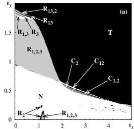
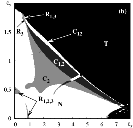
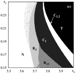
Figure 2: Regimes of extended starlike network (1) whose structure is shown in Fig. 1. Observe how areas of circular ($\mathbf{C}$) and radial ($\mathbf{R}$) clusters separate regimes with no synchronization ($\mathbf{N}$) and total synchronization ($\mathbf{T}$). (See explanation of subscripts in the text.) Natural frequencies of oscillators are given by Eq. (5). Bifurcation parameters in panels (a), (b) and (c) can be found in Eqs. (6), (7), and (8), respectively. Gray dashed line in panel (c) shows where Fig. 3 is drawn. Panel (d) represents enlarged central area of panel (a). In panels (e) and (f) bottom right and top left areas of panel (c) are shown.

Consider the star with $L=2$, $R=3$, whose structure is shown in Fig. 1. To observe the expected effects of clustering the natural frequencies of local oscillators have to be different. Otherwise the network merely tends to the synchronization of all nodes (also see Ref. [33] for the corresponding discussion). We assign the following values:

$$\omega_{1}=2.5,\;\omega_{2,4,6}=\{1.5,\;1.45,\;1.55\},\;\omega_{3,5,7}=\{1,\;0.95,\;1.05\},$$ (5)

i.e., the frequencies strongly decay from the hub to the periphery, and nodes located on identical distances from the hub have close but not coinciding frequencies.

Figure 2 shows charts of synchronization for the system (1), (5). Letters $\mathbf{N}$, $\mathbf{C}$, $\mathbf{R}$, and $\mathbf{T}$ signify areas of no synchronization, circular synchronization, radial synchronization, and total synchronization of the whole network, respectively. Subscript numbers of $\mathbf{R}$ denote the rays whose nodes are synchronized. Rays 1, 2, and 3 include nodes (2, 3), (4, 5), and (6, 7), respectively. Merged subscripts indicate that the corresponding rays are additionally synchronized with each other, while non-synchronized rays are separated by commas. Subscripts of $\mathbf{C}$ correspond to the distance from the hub and commas in the subscripts again separate clusters that are not synchronized with each other.

In Fig. 2(a) all bifurcation parameter are identical,

$$\mu_{1,\dots,7}=1.$$ (6)

We see that total synchronization occurs at the top right area of the chart. Except the total synchronization we also observe a large area of radial synchronization marked as $\mathbf{R_{1,2,3}}$, i.e., all nodes along each ray are synchronous but rays are not synchronized with each other. Also a small island of this regime appears near $\epsilon_{x}=1.2$, $\epsilon_{y}=0$. Regimes $\mathbf{R_{1,3}}$ and $\mathbf{R_{13}}$ are observed at the top left part of the figure. The former indicates synchronization of nodes siting on the first and the third rays, while the latter represents the case when these rays are additionally synchronized with each other. Synchronization along one ray only can also be observed: a very small stripe of $\mathbf{R_{3}}$ appears at the top left part of the plot, and $\mathbf{R_{2}}$ is observed in its lower area. Notice that since the star is not fully symmetric due to non-identical natural frequencies, see Eq. (5), the whole set of possible $\mathbf{R}$-regimes, e.g., $\mathbf{R_{2,3}}$ or $\mathbf{R_{12}}$, does not appear in the plot.

Circular synchronization in Fig. 2(a) is represented by a narrow stripes $\mathbf{C_{2}}$, $\mathbf{C_{1,2}}$, and $\mathbf{C_{12}}$. Enlarged this area is shown in Fig. 2(d). $\mathbf{C_{2}}$ indicates synchronization of far ends only. In area $\mathbf{C_{1,2}}$ both far ends and near-hub nodes are synchronized, but they are not synchronized with each other. Finally, in area $\mathbf{C_{12}}$ all nodes except the hub are synchronized.

These three regimes are the manifestations of so called remote synchronization, reported by Bergner et al. [33] for compact stars, i.e., with $L=1$. According to their explanation it emerges due to the transfer of signals of synchronized oscillators through the central node that operates like a filtering coupling line. Unlike their work, in our case a long-range version of the remote synchronization can be observed when the nodes interact through three node chains.

Figure 2(b) illustrates the case when the bifurcation parameter decays from the hub to far ends:

$$\mu_{1}=2,\;\mu_{2,4,6}=1.5,\;\mu_{3,5,7}=1.$$ (7)

Now areas $\mathbf{C_{2}}$, $\mathbf{C_{1,2}}$, and $\mathbf{C_{12}}$ get larger, while top left $\mathbf{R}$-areas almost vanishes. A tooth-like area $\mathbf{R_{1,2,3}}$ near $\epsilon_{x}=1.2$, $\epsilon_{y}=0$ observed in Fig. 2(a) is transformed into a belt around the origin. This belt is actually surrounded by small borders of $\mathbf{R_{1,2}}$, $\mathbf{R_{1,3}}$, $\mathbf{R_{2,3}}$, $\mathbf{R_{1}}$, and $\mathbf{R_{2}}$, however they are not shown due to their smallness.

In Fig. 2(c) the gradient of bifurcation parameter is higher:

$$\mu_{1}=3,\;\mu_{2,4,6}=2,\;\mu_{3,5,7}=1.$$ (8)

We see that areas of the remote synchronization $\mathbf{C_{2}}$, $\mathbf{C_{1,2}}$, and $\mathbf{C_{12}}$ are still well distinguishable, and their boundaries become more complicated: notice an island and a tongue of $\mathbf{C_{2}}$ in the central area of the plot; moreover notice a rib-like structure in its top left part. The belt $\mathbf{R_{1,2,3}}$ also still exists and gets larger.

Unlike panels (a) and (b) of Fig. 2 in the panel (c) a small area $\mathbf{C_{1}}$ appears near $\epsilon_{x}=6$, $\epsilon_{y}=0.2$. This is a one more manifestation of the remote synchronization where only near-hub nodes are synchronized, while both the hub and the far ends oscillate independently. In Fig. 2(e) this area is enlarged. In addition to areas $\mathbf{R_{3}}$, $\mathbf{R_{13}}$, and $\mathbf{C_{1}}$ we can distinguish here a stripe of $\mathbf{C_{1,2}}$.

A rib-like structure in top left area of Fig. 2(c) is enlarged in Fig. 2(f). We see that the ribs are formed by $\mathbf{R_{3}}$ areas, however there is one that corresponds to $\mathbf{C_{1}}$. Also notice various $\mathbf{R}$-regimes in the top area of the plot.

4 One parameter study of synchronization scenario

Using $q_{mn}$, see Eq. (4) we can estimate degrees of cluster synchronizations as follows:

$$q_{\text{rad}}^{(r)} =\frac{2}{L(L-1)}\sum_{m=1}^{L-1}\sum_{n=m+1}^{L}q_{1+(r-1)L+m,1+(r-1)L+n},\;1\leq r\leq R,$$ (9)

$$q_{\text{cir}}^{(\ell)} =\frac{2}{R(R-1)}\sum_{m=1}^{R-1}\sum_{n=m+1}^{R}q_{L(m-1)+\ell+1,L(n-1)+\ell+1},\;1\leq\ell\leq L,$$ (10)

$$q_{\text{prf}} =\frac{2}{(N-1)(N-2)}\sum_{m=2}^{N-1}\sum_{n=m+1}^{N}q_{m,n},$$ (11)

$$q_{\text{tot}} =\frac{2}{N(N-1)}\sum_{m=1}^{N-1}\sum_{n=m+1}^{N}q_{m,n}.$$ (12)

Here $q_{\text{rad}}^{(r)}$ stands for radial synchronization over $r$th ray, $q_{\text{cir}}^{(\ell)}$ shows the circular synchronization of peripherals nodes located on the distance $\ell$ from the hub, $q_{\text{prf}}$ shows the synchronization of all peripheral nodes except the hub, and, finally, $q_{\text{tot}}$ indicates the synchronization of the whole network. For example for the star shown in Fig. 1 $q_{\text{cir}}^{(1)}=(q_{2,4}+q_{2,6}+q_{4,6})/3$, $q_{\text{cir}}^{(2)}=(q_{3,5}+q_{3,7}+q_{5,7})/3$, $q_{\text{rad}}^{(1)}=q_{2,3}$, $q_{\text{rad}}^{(2)}=q_{4,5}$, $q_{\text{rad}}^{(3)}=q_{6,7}$.

Consider a scenario of transition to the total synchronization when the coupling strengths growth for the case shown in Fig. 2(c). We will vary $\epsilon_{y}$ and set $\epsilon_{x}=3\epsilon_{y}$, see the gray dashed line in this figure. Behavior of the criteria (9)-(12) along this line is represented in Figs. 3(a-c). Figure 3(d) demonstrates corresponding values of the first Lyapunov exponent.

Increasing the coupling strength we first observe the emergence of the radial synchronization at approximately $\epsilon_{y}=0.18$, see Fig. 3(a). It corresponds to the belt-like area $\mathbf{R_{1,2,3}}$ in Fig. 2(c). The curves of $q_{\text{rad}}^{(1)}$, $q_{\text{rad}}^{(2)}$ and $q_{\text{rad}}^{(3)}$ are located very close to each other but do not coincide entirely because natural frequencies of node oscillators are slightly different. Oscillations of different rays are not synchronized with each other. Otherwise $q_{\text{prf}}$ would also reach its maximum in Fig. 3(c) which actually does not take place.

Figure 3: Transition to total synchronization via cluster regimes as the coupling strength grows along the gray dashed line in Fig. 2(c). Panels (a), (b), and (c) shows synchronization criteria (9)-(12) and panel (d) represents the first Lyapunov exponent. Horizontal axis corresponds to $\epsilon_{y}$, $\epsilon_{x}=3\epsilon_{y}$, and other parameters correspond to Fig. 2(c).

Figure 4 shows Fourier spectra right below the point where $q_{\text{rad}}^{(r)}$ attains the maxima in Fig. 3(a). The first ray, i.e., nodes 1, 2, and 3, is represented. The spectra consist of series of isolated spikes that corresponds to a rich quasiperiodicity. The quasiperiodicity is also confirmed in Fig. 3(c) where the respective first Lyapunov exponent is zero. Quite different forms of spectra for $x_{1}$, $x_{2}$, and $x_{3}$, see Figs. 4(a), (b), and (c), respectively, is an obvious consequence of oscillators parameters mismatch.

Figure 4: Quasiperiodic oscillations right below the threshold of the radial synchronization indicated by the first maximum of $q_{\text{rad}}^{(1)}$, $q_{\text{rad}}^{(2)}$, and $q_{\text{rad}}^{(3)}$ in Fig. 3(a). Panels (a), (b) and (c) show Fourier spectra of $x_{1}$, $x_{2}$ and $x_{3}$, respectively. $\epsilon_{y}=0.16$. Quite different forms of spectra indicate an absence of synchronization.

The maximum of $q_{\text{rad}}^{(1)}$ at $\epsilon_{y}\approx 0.18$ in Fig. 3(a) indicates synchronization of the nodes 2 and 3. Figure 5(b) and (c) shows the corresponding Fourier spectra of these nodes. Observe their very high similarity. The spectra, however do not fully coincide since phase synchronous oscillations can be different in their detail structure. The forms of the spectra again, as in Fig. 4, indicate the quasiperiodic nature of the oscillations, and zero of the first Lyapunov exponent in Fig. 3(d) indicates the same. Comparing the spectra of peripheral nodes in Figs 5(b) and (c) with the hub spectrum represented in Fig 5(a), we see that all of them share a large number of harmonics. But the dominating frequency of the hub is different so that it remains independent from the peripheral nodes.

Figure 5: Quasiperiodicity at the point of emergence of the radial synchronization at $\epsilon_{y}=0.18$, see the first maximum of $q_{\text{rad}}^{(1)}$, $q_{\text{rad}}^{(2)}$, and $q_{\text{rad}}^{(3)}$ in Fig. 3(a). Panels (a), (b) and (c) represent Fourier spectra of $x_{1}$, $x_{2}$ and $x_{3}$, respectively. Due to the synchronization the spectra for nodes 2 and 3 share almost all harmonics. Non-synchronized hub, i.e, node 1, though reproduces some harmonics, has quite different dominating frequency.

Further growth of $\epsilon_{y}$ results in decay of $q_{\text{rad}}^{(r)}$, see Fig. 3(a), indicating the destruction of the radial synchronization. Corresponding Lyapunov exponent in Fig. 3(d) becomes positive. This is a footprint of the transition to chaos via destruction of multidimensional torus. This scenario is called as Landau-Hopf transition to chaos [41, 42, 43, 44, 45, 46, 47, 48, 49, 50]. Figure 6 shows Fourier spectra when the first Lyapunov has the maximum at $\epsilon_{y}\approx 0.42$. Instead of the separated spikes observed in Fig. 5, the spectra are now continuous that is a specific feature of chaos. The spectra of $x_{2}$ and $x_{3}$, see Figs. 5(b) and (c), respectively, are still similar to each other. The corresponding value of $q_{\text{rad}}^{(1)}$ is accordingly close to one. It means that despite the destruction of the radial synchronization, some degree of coherence of oscillations survives.

Figure 6: Chaos emerged as result of destruction of radial synchronization. Coupling parameter $\epsilon_{y}=0.42$ corresponds to the highest spike of $\lambda_{1}$ in Fig. 3(d). Panels (a), (b) and (c) represent Fourier spectra of $x_{1}$, $x_{2}$ and $x_{3}$, respectively. The spectra for nodes 2 and 3 are still similar, i.e., despite the destruction of the radial synchronization, some degree of coherence survives.

Subsequent growth of $\epsilon_{y}$ results in the destruction of chaos and reappearance of the quasiperiodicity, see Fourier spectra in Fig. 7 plotted at $\epsilon_{y}=0.5$. In comparison with the situation below the chaotic window, see Fig. 5, the reborn quasiperiodicity has much less number of independent frequencies. The reborn quasiperiodicity appears due to the transition to circular synchronization of far-end nodes 3, 5, and 7. Figure 7 corresponds to the edge of the island $\mathbf{C_{2}}$ in Fig. 2(c). This is a manifestation of long-range remote synchronization. The short-range version of this effect for compact stars with $L=1$ is reported by Bergner et al. [33]. This effect occurs since intermediate nodes operate like filtering communication lines [33]. In our case both the hub 1 and the near-hub nodes 2, 4, 6 operate like this. This is illustrated in Fig. 7 that shows how the essential harmonics of the far-end node 3 appear also in spectra of oscillations in the central nodes 1 and 2.

Figure 7: Reborn quasiperiodicity beyond chaotic regime and transition to circular synchronization of far ends at $\epsilon_{y}=0.5$, see Fig. 3(b) where $q_{\text{cir}}^{(2)}=1$ at this point. Panels (a), (b) and (c) represent Fourier spectra of $x_{1}$, $x_{2}$ and $x_{3}$, respectively. Synchronization of far end is provided by information transfer through central nodes: observe that the essential harmonics of the far-end node 3 appear also in spectra of nodes 1 and 2.

Fourier spectra for the edge of the main area $\mathbf{C_{2}}$ is shown in Fig. 8. Observe almost identical spectra in the panels (b), (c) and (d) corresponding to the synchronized nodes 3, 5 and 7. Notice that the essential harmonics of these nodes are present in the hub oscillations, panel (a), but the hub dominating frequency differs from that of far ends.

Figure 8: Circular synchronizations of far ends at $\epsilon_{y}=1$. Panels (a),(b),(c), and (d) represent Fourier spectra of nodes $x_{1}$, $x_{3}$, $x_{5}$ and $x_{7}$, respectively. Observe almost identical spectra of far end nodes 3, 5, and 7. The essential harmonics of these nodes also present in the hub spectrum, but the dominating frequency differs.

Further increment of $\epsilon_{y}$ results in the emergence of one more form of the remote synchronization. In addition to far-end cluster near-hub nodes are also get synchronized. In Fig. 3(b) $q_{\text{cir}}^{(1)}=1$ at $\epsilon_{y}\approx 1.1$. Since $q_{\text{prf}}<1$ in Fig. 3(c), far-end and near-hub clusters oscillate independently. Figure 9 compares Fourier spectra of the nodes 2 and 3 at $\epsilon_{y}=1.2$ when they are involved into different synchronization clusters, see area $\mathbf{C_{1,2}}$ in Fig. 2(c). Though the dominating frequencies are the same, the amplitudes of other harmonics are different. The high similarity of spectra contents is explained by a twofold role of the near-hub nodes in this case. In addition to their own oscillations they provide the coupling line for far ends.

Figure 9: Independent clusters of near-hub and far-end nodes at $\epsilon_{y}=1.2$. Panels (a) and (b) show Fourier spectra of $x_{2}$, $x_{3}$, respectively. Though nodes 2 and 3 belong to clusters that are not synchronized with each other, their spectra are highly similar. This is explained by a twofold role of the near-hub node 2: in addition to its own oscillations, it provides the coupling line for the far-end node 3.

Subsequent growth of $\epsilon_{y}$ results in the synchronization of both circular clusters, so that all nodes except the hub are synchronized. In Fig. 3(c) $q_{\text{prf}}=1$ at $\epsilon_{y}\approx 1.3$. Obviously this is the third observed form of the remote synchronization. The hub gets involved into synchronization at $\epsilon_{y}\approx 1.4$, see Fig. 3(c), so that the whole network becomes synchronized.

5 Charts of sychronization for lager stars

a)  b)  c) 

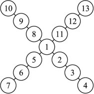
Figure 10: Starlike networks with (a) $L=2$, $R=4$; (b) $L=3$, $R=3$; (c) $L=3$, $R=4$.

Figure 11: Synchronization charts for starlike networks with (a) $L=2$, $R=4$; (b) $L=3$, $R=3$; (c) $L=3$, $R=4$, see Fig. 10. Observe that the number of rays $R$ does not influence much the overall structure of the chart, compare panel (a) with Fig. 2(c) and panel (b) with (c). The ray length $L$ however changes the picture dramatically.

Let us now consider stars whose rays are longer and their number is higher, see Fig. 10. Figure 10(a) shows the star with $R=4$, $L=2$, i.e., it has one more ray in comparison with Fig. 1. Similarly to the previous case natural frequencies of the oscillators, see Eq. (1), strongly decay from the hub to the periphery:

$$\omega_{1}=2.5,\;\omega_{2,4,6,8}=\{1.475,1.525,1.425,1.575\},\;\omega_{3,5,7,9}=\{0.975,1.025,0.925,1.075\}.$$ (13)

Bifurcation parameters correspond to Fig. 2(c), see Eq. (8):

$$\mu_{1}=3,\;\mu_{2,4,6,8}=2,\;\mu_{3,5,7,9}=1.$$ (14)

Figure 11(a) shows the chart of synchronization for this star. The charts for $R=3$, $L=2$ in Fig. 2(c) and for $R=4$, $L=2$ in 11(a) are very similar to each other. Areas of total synchronization $\mathbf{T}$ are almost identical. In both cases transition to it occurs via circular synchronization $\mathbf{C_{2}}$, $\mathbf{C_{1,2}}$ and $\mathbf{C_{12}}$. The belt of radial synchronization $\mathbf{R_{1,2,3}}$ located near the origin in Fig. 2(c) coincide with the belt $\mathbf{R_{1,2,3,4}}$ in Fig. 11(a). Finally, the convexity of $\mathbf{T}$ in bottom right parts in both cases are surrounded by a border of $\mathbf{C_{1}}$ and by a few $\mathbf{R}$-areas. Thus we observe that the global structure of synchronization charts is rather insensitive to the number of the rays.

Increase of the ray length $L$ results in dramatic changings. Figs. 10(b) and (c) show two stars with $L=3$ whose numbers of rays are $R=3$ and $R=4$, respectively. We set the following parameters for $R=3$:

$$\omega_{1}=4,\;\omega_{2,5,8}=\{2.5,2.45,2.55\},\;\omega_{3,6,9}=\{1.6,1.55,1.65\},\;\omega_{4,7,10}=\{0.7,0.65,0.75\},$$ (15)

$$\mu_{1}=3,\;\mu_{2,5,8}=2,\;\mu_{3,6,9}=1,\;\mu_{4,7,10}=0.5,$$ (16)

and for $R=4$:

$$\begin{gathered}\omega_{1}=4,\;\omega_{2,5,8,11}=\{2.475,2.525,2.425,2.575\},\;\\ \omega_{3,6,9,12}=\{1.575,1.625,1.525,1.675\},\;\omega_{4,7,10,13}=\{0.675,0.725,0.625,0.775\},\end{gathered}$$ (19)

$$\mu_{1}=3,\;\mu_{2,5,8}=2,\;\mu_{3,6,9}=1,\;\mu_{4,7,10}=0.5.$$ (20)

Figs. 11(b) and (c) represent the synchronization charts for $L=3$, $R=3$ and $L=3$, $R=4$, respectively. First of all notice that the these two charts are strongly different from the case $L=2$, cf. with Figs. 2(c) and 11(a). Moreover observe their high similarity: compare areas $\mathbf{C_{2,3}}$, $\mathbf{C_{2}}$, $\mathbf{C_{3}}$, $\mathbf{C_{1,2,3}}$, $\mathbf{C_{12,3}}$,$\mathbf{C_{12}}$ $\mathbf{C_{123}}$, and, finally $\mathbf{T}$. Unlike the case $L=2$, large $\mathbf{R}$ areas are absent. Instead there are areas $\mathbf{C_{1}R}$ where synchronized near-hub nodes are also synchronized with several rays.

As discussed above, at $L=2$ the scenario of transition to the total synchronization via remote synchronization includes regimes $\mathbf{C_{2}}$, $\mathbf{C_{1,2}}$, and $\mathbf{C_{12}}$, see Figs. 2(c) and 11(a). In other words, far ends get synchronized first, then near-hub nodes also become synchronous, then these two clusters merges, and, finally the hub also get involved so that the whole network oscillates synchronously. This scenarios survives at $L=3$ with an obvious modification due to longer rays. In the right parts of the charts in Figs. 11(b) and (c) we observe that far ends get synchronized first, area $\mathbf{C_{3}}$. Then goes area $\mathbf{C_{2,3}}$, i.e., there are two independent clusters including far ends and intermediate nodes. Subsequent area is $\mathbf{C_{1,2,3}}$ which means that all peripheral nodes belong to circular clusters and they are not synchronized with each other. Area $\mathbf{C_{12,3}}$ is located further. Here near-hub nodes remain independent, while far ends and intermediate nodes are merged into a single cluster. The final area before the total synchronization is a very thin stripe of $\mathbf{C_{123}}$. It represents the synchronization of all peripheral nodes.

Altogether, comparison of the charts in Figs. 2 and 11 allows to conclude that the ray length $L$ dramatically influences the synchronization scenario in extended starlike networks, whereas higher the ray number $R$ merely brings more fine details in the picture. Moreover, the increase of $L$ results in enrichment of the variety of manifestations of the remote synchronization. In particular, at $L=3$ sole far ends get synchronized being connected by non-synchronized five node paths.

6 Asymmetric star

Let us now consider an asymmetric star. To perform a comparison we take a network shown in Fig. 10(b), whose parameters are given by Eqs. (15) and (16), and cut off its last node 10. The resulting asymmetric network is shown in Fig. 12(a).

Figure 12(b) represents a synchronization chart for the asymmetric star, and the chart for the corresponding uncut star is in Fig. 11(b). We observe that the removing of one peripheral node results in the total reorganization of the pictures. Fully symmetric case in Fig. 11(b) is dominated by circular clusters, while radial ones emerge only together with $\mathbf{C_{1}}$.

Cutting the node results in the vanish of the most of circular clusters and emerging of areas of radial clusters instead. It occurs because nodes involved in the circular clusters are located symmetrically with respect to rotations of the network around the hub. The lack of topology symmetry results in the destruction of these symmetry related clusters. Also this is the case for the total synchronization regime that shrinks when the topology symmetry is damaged: compare areas $\mathbf{T}$ in Figs. 11(b) and 12(b). The radial clusters, on the contrary, are not related to the topology symmetry so that its lack accompanied with the vanish of circular clusters benefits to them.

Notice that the long-range remote synchronization does not fully vanish in the asymmetric case. In Fig.12(b) we can see three large areas of clusters $\mathbf{C_{3}}$. For the considered network, see Fig. 12(a), it means that nodes 4 and 7 are synchronized while other oscillate independently. For the symmetric stars we discussed above the scenario of transition to the total synchronization via one by one formation of circular clusters from far ends to the hub. In the asymmetric case we can also observe similar situation. As follows from Fig. 12(b) if $\epsilon_{y}$ grows at constant small $\epsilon_{x}$ far ends get synchronized first and, after that, the whole network become synchronous. On the boundary between areas $\mathbf{C_{3}}$ and $\mathbf{T}$ there is very narrow stripe of other circular clusters. However, we do not highlight it in the plot since it is barely visible.

a)   

Figure 12: Asymmetric star, panel (a), cf. with Fig. 10(b), and corresponding synchronization chart, panel (b), cf. with Fig. 11(b). Cutting off one node results in total reorganization of the chart. Circular clusters mainly vanish in favor of radial ones. Nevertheless, long-range remote synchronization survives, see areas $\mathbf{C_{3}}$.

7 Amplitude equations

To verify typical nature of circular and radial cluster synchronizations, consider amplitude equations for the network (1). They are also known as Stuart-Landau equations [13]. Their derivation in our case is basically straightforward. According to the standard routine [13], it is assumed that solution can be represented as a fast harmonic oscillation with slow amplitude modulation. Taking identical for all nodes fast component with frequency $\omega_{1}$, we obtain the assumed solution:

$$x_{n}(t)=A_{n}\mathrm{e}^{\mathrm{i}\mkern 1.0mu\omega_{1}t}+A^{*}_{n}\mathrm{e}^{-\mathrm{i}\mkern 1.0mu\omega_{1}t},$$ (21)

where $A_{n}\equiv A_{n}(t)$ is a slow varying complex amplitude and $A^{*}_{n}$ is its complex conjugation. After substitution Eq. (21) to Eq. (1) we apply the standard auxiliary condition

$$\dot{A}_{n}\mathrm{e}^{\mathrm{i}\mkern 1.0mu\omega_{1}t}+\dot{A}^{*}_{n}\mathrm{e}^{-\mathrm{i}\mkern 1.0mu\omega_{1}t}=0,$$ (22)

and average resulting equations over fast components. Finally, we rescale time as $t\to 2t$ to eliminate insignificant factor 2, and obtain a sought network of amplitude equations:

$$\dot{A}_{n}=\left(\mu_{n}+\mathrm{i}\mkern 1.0mu\frac{\omega_{n}^{2}-\omega_{1}^{2}}{\omega_{1}}\right)A_{n}-A_{n}|A_{n}|^{2}+\left(\epsilon_{y}-\mathrm{i}\mkern 1.0mu\frac{\epsilon_{x}}{\omega_{1}}\right)\left(\sum_{j=1}^{N}\frac{a_{nj}}{k_{n}}A_{j}-A_{n}\right).$$ (23)

At $\epsilon_{x}=0$ and $\mu_{1}=\mu_{2}=\cdots=\mu_{n}=\mu$ Eq. (23) turns to the network used by Bergner et al. [33] to study the remote synchronization.

We consider a starlike network of amplitude equations (23) with $L=2$, $R=3$, see Fig. 1. Parameters are taken with noticeable gradients both in $\omega$ and $\mu$:

$$\omega_{1}=1,\;\omega_{2,4,6}=\{0.8,\;0.75,\;0.85\},\;\omega_{3,5,7}=\{0.6,\;0.55,\;0.65\},$$ (24)

$$\mu_{1}=1,\;\mu_{2,4,6}=0.8,\;\mu_{3,5,7}=0.6.$$ (25)

Synchronization chart is shown in Fig. 13. Analogous parameter set with noticeable gradients, see Eqs. (5) and (8), is employed for the original system (1) in Fig. 2(c). We can see that the charts in Figs. 13 and 2(c) have many similar features. In both cases areas $\mathbf{T}$ of total synchronization are located in the top right parts and separated from areas $\mathbf{N}$ where no synchronization occurs by stripes of circular clusters. First goes $\mathbf{C_{2}}$, i.e., only far ends are synchronized, then near-hub nodes also become synchronous without synchronization with the far ends, $\mathbf{C_{1,2}}$, after that both circular clusters become synchronous, $\mathbf{C_{12}}$, and, finally, total synchronization takes place, $\mathbf{T}$. In both cases these stripes are furrowed by the rib-like structures. Also there are large bulges of total synchronization in the bottom right parts of the charts. Finally, both charts contains islands of radial synchronization that, however, are not located in somehow similar ways.

It is well known that the considered amplitude equations are universal models for a wide class of self-oscillators with supercritical Hopf bifurcation. Thus, observed similarity of charts in Fig. 13 and 2(c) indicates that circular clusters and long-range remote synchronization as well as radial clusters are typical and robust phenomena of starlike networks of self-oscillators of mentioned type.

Figure 13: Synchronization chart for amplitude equations (23) on the star at $L=2$, $R=3$, see Fig. 1. Overall structure of the chart is similar to that one for van der Pol oscillators, cf. with Fig. 2(c).

8 Conclusion

In this paper we considered an extended starlike network of nonidentical self-oscillators in presence of both reactive and dissipative coupling. These networks demonstrated two types of synchronization clusters which were radial and circular. Radial synchronization cluster involves all nodes along a ray, while circular synchronization cluster consists of nodes from all rays located on the same distance form the hub. By the nature, circular clusters are the long-range version of so called remote synchronization. Their feature is that the involved nodes do not have a direct connections and interact only through intermediary nodes.

Various forms of long-range remote synchronization can be treated as elements of scenario of transition to the total synchronization of the network. We observed that the far ends of rays synchronized first. Then more circular clusters appeared involving closer to hub nodes. Subsequently the clusters merged and, finally, all network became synchronous.

Behavior of the extended starlike networks was found to be strongly determined by the ray length. Its increment resulted in dramatic rearrangement of the considered synchronization charts. Varying of the number of rays, however, affected basically the fine details of the charts while their coarse grain structure remained unaltered.

Furthermore, we observed that the dynamics essentially depends on the underlying topology symmetry. It can be treated as one more manifestation of the dependence on the ray length. When one ray terminating node was removed, so that the star became asymmetric, the synchronization chart changed very seriously. Most of circular clusters, related by their nature to the network symmetry, vanished, while more radial clusters appeared instead. Nevertheless, asymmetry did not totally killed the long-range remote synchronization. The chart for asymmetric star contained large ares where the far end nodes were synchronized while all others oscillated independently.

We considered networks of van der Pol oscillators and corresponding amplitude equations that are known as a universal model for a wide class of self-oscillators. Inspected synchronization charts for this two types of dynamical systems showed high qualitative similarity: circular and radial clusters were detected in both cases, and moreover overall structures of the charts were mainly similar. This is a serious argument in favor of typical nature of the reported phenomena for self-oscillators.

To observe the reported variety of phenomena the natural frequencies of the oscillators were taken decaying from the hub node along rays. The nodes located on the same distances from the hub had close but also nonidentical natural frequencies. Multiple simulations indicated that this is a sufficient condition for the circular clusters to appear. It agrees with the paper by Bergner et al. [33] who study a remote synchronization choosing natural frequencies in the similar way. Tried bifurcation parameters were totally identical as well as decaying along rays. Circular clusters appeared in both cases, however the second choice was more preferable since the areas of their existence on a synchronization chart became larger. As for the radial clusters, they obviously prefer identical or close parameters along rays. However we observed that they still could emerge when the parameters were sufficiently different. These considerations of the parameters choice are rather empirical. More rigorous conditions should be the subject of further studies.

This work was partially (P.V.K.) supported by RFBR Grant No. 16-02-00135

References

- [1] A.-L. Barabási, R. Albert, Emergence of scaling in random networks, Science 286 (5439) (1999) 509–512. doi:10.1126/science.286.5439.509.
- [2] R. K. Merton, The matthew effect in science, Science 159 (3810) (1968) 56–63. doi:10.1126/science.159.3810.56.
- [3] A.-L. Barabási, Network science, Cambridge University Press, 2016.
- [4] S. Boccaletti, V. Latora, Y. Moreno, M. Chavez, D.-U. Hwang, Complex networks: Structure and dynamics, Physics Reports 424 (4-5) (2006) 175–308. doi:10.1016/j.physrep.2005.10.009.
- [5] X. F. Wang, Complex networks: topology, dynamics and synchronization, International Journal of Bifurcation and Chaos 12 (05) (2002) 885–916. doi:10.1142/S0218127402004802.
- [6] M. Perc, The matthew effect in empirical data, Journal of The Royal Society Interface 11 (98) (2014) 20140378. doi:10.1098/rsif.2014.0378.
- [7] R. Albert, Scale-free networks in cell biology, Journal of Cell Science 118 (21) (2005) 4947–4957. doi:10.1242/jcs.02714.
- [8] R. Dobrescu, F. Ionescu, Large Scale Networks: Modeling and Simulation, CRC Press, 2016.
- [9] A.-L. Barabási, R. Albert, H. Jeong, Scale-free characteristics of random networks: the topology of the world-wide web, Physica A 281 (1-4) (2000) 69–77. doi:10.1016/S0378-4371(00)00018-2.
- [10] I. Sohn, Small-world and scale-free network models for IoT systems, Mobile Information Systems 2017, article ID 6752048, 9 pages. doi:10.1155/2017/6752048.
- [11] G. Bianconi, C. Rahmede, Emergent hyperbolic network geometry, Scientific Reports 7 (2017) 41974. doi:10.1038/srep41974.
- [12] G. Bianconi, Interdisciplinary and physics challenges of network theory, EPL (Europhysics Letters) 111 (5) (2015) 56001.
- [13] A. Pikovsky, M. Rosenblum, J. Kurths, Synchronization, Cambridge University Press, 2003.
- [14] A. Arenas, A. Díaz-Guilera, J. Kurths, Y. Moreno, C. Zhou, Synchronization in complex networks, Physics Reports 469 (3) (2008) 93 – 153. doi:10.1016/j.physrep.2008.09.002.
- [15] G. V. Osipov, J. Kurths, C. Zhou, Synchronization in oscillatory networks, Springer Science & Business Media, 2007.
- [16] M. Golubitsky, I. Stewart, Recent advances in symmetric and network dynamics, Chaos: An Interdisciplinary Journal of Nonlinear Science 25 (9) (2015) 097612. doi:10.1063/1.4918595.
- [17] I. Belykh, M. Hasler, M. Lauret, H. Nijmeijer, Synchronization and graph topology, International Journal of Bifurcation and Chaos 15 (11) (2005) 3423–3433. doi:10.1142/S0218127405014143.
- [18] A. Arenas, A. Díaz-Guilera, C. J. Pérez-Vicente, Synchronization reveals topological scales in complex networks, Phys. Rev. Lett. 96 (2006) 114102. doi:10.1103/PhysRevLett.96.114102.
- [19] X. F. Wang, G. Chen, Synchronization in scale-free dynamical networks: robustness and fragility, Circuits and Systems I: Fundamental Theory and Applications, IEEE Transactions on 49 (1) (2002) 54–62. doi:10.1109/81.974874.
- [20] J. Fan, X. F. Wang, On synchronization in scale-free dynamical networks, Physica A: Statistical Mechanics and its Applications 349 (3–4) (2005) 443 – 451. doi:10.1016/j.physa.2004.09.016.
- [21] S. Jalan, A. Singh, S. Acharyya, J. Kurths, Impact of a leader on cluster synchronization, Phys. Rev. E 91 (2015) 022901. doi:10.1103/PhysRevE.91.022901.
- [22] X. F. Wang, G. Chen, Pinning control of scale-free dynamical networks, Physica A: Statistical Mechanics and its Applications 310 (3–4) (2002) 521 – 531. doi:http://dx.doi.org/10.1016/S0378-4371(02)00772-0.
- [23] P. V. Kuptsov, U. Parlitz, Theory and computation of covariant Lyapunov vectors, J. Nonlinear Sci. 22 (5) (2012) 727–762. doi:10.1007/s00332-012-9126-5.
- [24] P. V. Kuptsov, A. V. Kuptsova, Predictable nonwandering localization of covariant lyapunov vectors and cluster synchronization in scale-free networks of chaotic maps, Phys. Rev. E 90 (2014) 032901. doi:10.1103/PhysRevE.90.032901.
- [25] W. Li, C. Li, H. Song, Quantum synchronization and quantum state sharing in an irregular complex network, Phys. Rev. E 95 (2017) 022204. doi:10.1103/PhysRevE.95.022204.
- [26] L. M. Pecora, Synchronization conditions and desynchronizing patterns in coupled limit-cycle and chaotic systems, Phys. Rev. E 58 (1998) 347–360. doi:10.1103/PhysRevE.58.347.
- [27] Z. Ma, G. Zhang, Y. Wang, Z. Liu, Cluster synchronization in star-like complex networks, Journal of Physics A: Mathematical and Theoretical 41 (15) (2008) 155101. doi:10.1088/1751-8113/41/15/155101.
- [28] P. V. Kuptsov, A. V. Kuptsova, Variety of regimes of starlike networks of Hénon maps, Phys. Rev. E 92 (2015) 042912. doi:10.1103/PhysRevE.92.042912.
- [29] P. V. Kuptsov, A. V. Kuptsova, Cluster synchronization of starlike networks with normalized Laplacian coupling: master stability function approach, Proc. of SPIE 9917 (2016) 99173O. doi:10.1117/12.2229780.
- [30] R. Chacón, F. Palmero, J. Cuevas-Maraver, Impulse-induced localized control of chaos in starlike networks, Phys. Rev. E 93 (2016) 062210. doi:10.1103/PhysRevE.93.062210.
- [31] J. Wang, Y. Zhang, Network synchronization in a population of star-coupled fractional nonlinear oscillators, Physics Letters A 374 (13-14) (2010) 1464–1468. doi:10.1016/j.physleta.2010.01.042.
- [32] A. Hutton, S. Bose, Mediated entanglement and correlations in a star network of interacting spins, Phys. Rev. A 69 (2004) 042312. doi:10.1103/PhysRevA.69.042312.
- [33] A. Bergner, M. Frasca, G. Sciuto, A. Buscarino, E. J. Ngamga, L. Fortuna, J. Kurths, Remote synchronization in star networks, Phys. Rev. E 85 (2012) 026208. doi:10.1103/PhysRevE.85.026208.
- [34] I. Fischer, R. Vicente, J. M. Buldú, M. Peil, C. R. Mirasso, M. C. Torrent, J. García-Ojalvo, Zero-lag long-range synchronization via dynamical relaying, Phys. Rev. Lett. 97 (2006) 123902. doi:10.1103/PhysRevLett.97.123902.
- [35] R. Gutiérrez, R. Sevilla-Escoboza, P. Piedrahita, C. Finke, U. Feudel, J. M. Buldú, G. Huerta-Cuellar, R. Jaimes-Reátegui, Y. Moreno, S. Boccaletti, Generalized synchronization in relay systems with instantaneous coupling, Phys. Rev. E 88 (2013) 052908. doi:10.1103/PhysRevE.88.052908.
- [36] L. V. Gambuzza, M. Frasca, L. Fortuna, S. Boccaletti, Inhomogeneity induces relay synchronization in complex networks, Phys. Rev. E 93 (2016) 042203. doi:10.1103/PhysRevE.93.042203.
- [37] L. V. Gambuzza, A. Cardillo, A. Fiasconaro, L. F. J. Gomez-Gardenes, M. Frasca, Analysis of remote synchronization in complex networks, Chaos 23 (2013) 043103. doi:10.1063/1.4824312.
- [38] V. Nicosia, M. Valencia, M. Chavez, A. Díaz-Guilera, V. Latora, Remote synchronization reveals network symmetries and functional modules, Phys. Rev. Lett. 110 (2013) 174102. doi:10.1103/PhysRevLett.110.174102.
- [39] S. Jalan, R. E. Amritkar, Self-organized and driven phase synchronization in coupled maps, Phys. Rev. Lett. 90 (2003) 014101. doi:10.1103/PhysRevLett.90.014101.
- [40] S. Jalan, R. E. Amritkar, C.-K. Hu, Synchronized clusters in coupled map networks. i. numerical studies, Phys. Rev. E 72 (2005) 016211. doi:10.1103/PhysRevE.72.016211.
- [41] P. M. Battelino, Persistence of three-frequency quasiperiodicity under large perturbations, Phys. Rev. A 38 (1988) 1495–1502. doi:10.1103/PhysRevA.38.1495.
- [42] P. Ashwin, G. P. King, J. W. Swift, Three identical oscillators with symmetric coupling, Nonlinearity 3 (3) (1990) 585. doi:10.1088/0951-7715/3/3/003.
- [43] P. Ashwin, J. Guaschi, J. Phelps, Rotation sets and phase-locking in an electronic three oscillator system, Physica D: Nonlinear Phenomena 66 (3) (1993) 392 – 411. doi:10.1016/0167-2789(93)90075-C.
- [44] V. Anishchenko, S. Nikolaev, J. Kurths, Peculiarities of synchronization of a resonant limit cycle on a two-dimensional torus, Phys. Rev. E 76 (2007) 046216. doi:10.1103/PhysRevE.76.046216.
- [45] V. Anishchenko, S. Astakhov, T. Vadivasova, Phase dynamics of two coupled oscillators under external periodic force, EPL (Europhysics Letters) 86 (3) (2009) 30003. doi:10.1209/0295-5075/86/30003.
- [46] A. Kuznetsov, I. Sataev, L. Turukina, On the road towards multidimensional tori, Communications in Nonlinear Science and Numerical Simulation 16 (6) (2011) 2371 – 2376. doi:10.1016/j.cnsns.2010.09.026.
- [47] Y. Emelianova, A. Kuznetsov, I. Sataev, L. Turukina, Synchronization and multi-frequency oscillations in the low-dimensional chain of the self-oscillators, Physica D: Nonlinear Phenomena 244 (1) (2013) 36 – 49. doi:10.1016/j.physd.2012.10.012.
- [48] R. Van Buskirk, C. Jeffries, Observation of chaotic dynamics of coupled nonlinear oscillators, Phys. Rev. A 31 (1985) 3332–3357. doi:10.1103/PhysRevA.31.3332.
- [49] V. S. Anishchenko, S. M. Nikolaev, Transition to chaos from quasiperiodic motions on a four-dimensional torus perturbed by external noise, International Journal of Bifurcation and Chaos 18 (09) (2008) 2733–2741. doi:10.1142/S0218127408021956.
- [50] A. P. Kuznetsov, S. P. Kuznetsov, I. R. Sataev, L. V. Turukina, About Landau-Hopf scenario in a system of coupled self-oscillators, Physics Letters A 377 (45-48) (2013) 3291 – 3295. doi:10.1016/j.physleta.2013.10.013.