Co-evolutionary multi-task learning for dynamic time series prediction

Abstract

Time series prediction typically consists of a data reconstruction phase where the time series is broken into overlapping windows known as the timespan. The size of the timespan can be seen as a way of determining the extent of past information required for an effective prediction. In certain applications such as the prediction of wind-intensity of storms and cyclones, prediction models need to be dynamic in accommodating different values of the timespan. These applications require robust prediction as soon as the event takes place. We identify a new category of problem called dynamic time series prediction that requires a model to give prediction when presented with varying lengths of the timespan. In this paper, we propose a co-evolutionary multi-task learning method that provides a synergy between multi-task learning and co-evolutionary algorithms to address dynamic time series prediction. The method features effective use of building blocks of knowledge inspired by dynamic programming and multi-task learning. It enables neural networks to retain modularity during training for making a decision in situations even when certain inputs are missing. The effectiveness of the method is demonstrated using one-step-ahead chaotic time series and tropical cyclone wind-intensity prediction.

1 Introduction

Time series prediction typically involves a pre-processing stage where the original time series is reconstructed into a state-space representation that is used as dataset for training models such as neural networks [1, 2, 3, 4, 5, 6, 7, 8]. The reconstruction involves breaking the time series using overlapping windows known as timespan taken at regular intervals which defines the time lag [9]. The optimal values for timespan and time lag are needed for effective prediction. These values vary on the type of problem and require costly computational evaluation for model selection; hence, some effort has been made to address this issue. Multi-objective and competitive coevolution methods have been used to take advantage of different features from the timespan during training [10, 11]. Moreover, neural network have been used for determining optimal timespan of selected time series problems [12].

In time series for natural disasters such as cyclones [13, 14, 15], it is important to develop models that can make predictions dynamically, i.e. the model has the ability to make a prediction as soon as any observation or data is available. The minimal value for the timespan can have huge impact for the case of cyclones, where data is only available every 6 hours [16]. A way to address such categories of problems is to devise robust training algorithms and models that are capable of performing given different types of input or subtasks. We define dynamic time series prediction as a problem that requires dynamic prediction given a set of input features that vary in size. It has been highlighted in recent work [16] that recurrent neural networks trained with a predefined timespan can only generalise well for the same timespan which makes dynamic time series prediction a challenging problem. Time series prediction problems can be generally characterised into three major types of problems that include one-step [3, 2, 7], multi-step-ahead [17, 18, 19], and multi-variate time series prediction [20, 21, 22]. These problems at times may overlap with each other, for instance, a multi-step-ahead prediction can have a multi-variate component. Similarly, a one-step prediction can also have a multi-variate component, or a one-step ahead prediction can be used for multi-step prediction and vice-versa. In this paper, we identify a special class of problems that require dynamic prediction with the hope that the trained model can be useful for different instances of the problem.

Multi-task learning employs shared representation knowledge for learning multiple instances from the same problem with the goal to develop models with improved performance in decision making [23, 24, 25, 26]. We note that different values in the timespan can be used to generate several distinct datasets that have overlapping features which can be used to train modules for shared knowledge representation as needed for multi-task learning. Hence, it is important to ensure that modularity is retained in such a way so that decision making can take place even when certain inputs are missing. Modular neural networks have been motivated from repeating structures in nature and applied for visual recognition tasks [27]. Neuroevolution has been used to optimise performance and connection costs in modular neural networks [28] which also has the potential of learning new tasks without forgetting old ones [29]. The features of modular learning provide motivation to be incorporated with multi-task learning for dynamic time series prediction.

In dynamic programming, a large problem is broken down into sub-problems, from which at least one sub-problem is used as a building block for the optimisation problem. Although dynamic programming has been primarily used for optimisation problems, it has been briefly explored for data driven learning [30] [31]. The notion of using sub-problems as building block in dynamic programming can be used in developing algorithms for multi-task learning. Cooperative coevolution (CC) is a divide and conquer approach that divides a problem into subcomponents that are implemented as sub-populations [32]. CC has been effective for learning difficult problems using neural networks [33]. Potter and De Jong demonstrated that CC provides more diverse solutions through the sub-populations when compared to conventional evolutionary algorithms [33]. CC has been very effective for training recurrent neural networks for time series prediction problems [7, 8].

Although multi-task learning has mainly been used for machine learning problems, the concept of shared knowledge representation has motivated other domains. In the optimisation literature, multi-task evolutionary algorithms have been proposed for exploring and exploiting common knowledge between the tasks and enabling transfer of knowledge between them for optimisation [34, 35]. It was demonstrated that knowledge from related tasks can help in speeding up the optimisation process and obtain better quality solutions when compared to conventional (single-task optimisation) approaches. Evolutionary multi-task learning has been used for efficiently training feedforward neural networks for $n$-bit parity problem [36], where different subtasks were implemented as different topologies that obtained improved training performance. In the literature, synergy of dynamic programming, multi-task learning and neuroevolution has not been explored. Ensemble learning methods would be able to address dynamic time series to an extent, where an ensemble is defined by the timespan of the time series. Howsoever, it would not have the feature of shared knowledge representation that is provided through multi-task learning. Moreover, there is a need for a unified model for dynamic times series problems due to problems that require dynamic prediction.

In this paper, we propose a co-evolutionary multi-tasking method that provides a synergy between multi-task learning, dynamic programming and coevolutionary algorithms. The method enables neural networks to be trained by featuring shared and modular knowledge representation in order to make predictions given limited input features. This enables the learning process to employ modules of knowledge from the related subtasks as building blocks of knowledge for a unified model. The proposed method is used for one-step-ahead chaotic time series problems using feedforward neural networks for benchmark problems. The method is also used for tropical cyclone wind-intensity prediction and addresses the problem of minimal timespan where dynamic prediction is required. The paper extends results presented in [37].

The rest of the paper is organised as follows. Section 2 gives a background on multi-task learning, cooperative neuro-evolution, and time series prediction. Section 3 gives details of the co-evolutionary multi-task learning method for dynamic time series prediction. Section 4 presents the results with discussion and Section 5 presents the conclusions and directions for future research.

2 Background and Related Work

2.1 Multi-task learning and applications

A number of approaches have been presented that considers multi-task learning [23] for different types of problems that include supervised and unsupervised learning [38, 39, 40, 41]. The major approach to address negative transfer for multi-task learning has been through task grouping where knowledge transfer is performed only within each group [42, 43]. Bakker et al. for instance, presented a

Bayesian approach in which some of the model parameters were shared and others loosely connected through a joint prior distribution learnt from the data [43]. Zhang and Yeung presented a convex formulation for multi-task metric learning by modeling the task relationships in the form of a task covariance matrix [42]. Moreover, Zhong et al. presented flexible multi-task learning framework to identify latent grouping structures in order to restrict negative knowledge transfer [44]. Multi-task learning has recently contributed to a number of successful real-world applications that gained better performance by exploiting shared knowledge for multi-task formulation. Some of these applications include 1) multi-task approach for “ retweet” prediction behaviour of individual users [45], 2) recognition of facial action units [22], 3) automated Human Epithelial Type 2 (HEp-2) cell classification [46], 4) kin-relationship verification using visual features [47] and 5) object tracking [48].

2.2 Cooperative Neuro-evolution

Neuro-evolution employs evolutionary algorithms for training neural networks [49] which can be classified into direct [49, 50] and indirect encoding strategies [51]. In direct encoding, every connection and neuron is specified directly and explicitly in the genotype [49, 50]. In indirect encoding, the genotype specifies rules or some other structure for generating the network [51]. Performance of direct and indirect encodings varies for specific problems. Indirect encodings seem very intuitive and have biological motivations, however, in several cases they have shown not to outperform direct encoding strategies [52, 53].

Cooperative coevolution for training neural networks is known as cooperative neuroevolution [33, 54, 55]. Although cooperative coevolution faced challenges in problem decomposition, it showed promising features that included modularity and diversity [33]. Further challenges have been in area of credit assignment for subcomponents [33, 54], problem decomposition, and adaptation due to problem of separability that refer to grouping interacting or highly correlated variables [55]. In cooperative neuro-evolution, problem decomposition has a major effect in the training and generalisation performance. Although several decomposition strategies have been implemented that vary for different network architectures, the two established decomposition methods are those on the synapse [52] and neuron level [56, 55, 57]. In synapse level, the network is decomposed to its lowest level where each weight connection (synapse) forms a subcomponent [52, 6]. In neuron level, the neurons in the network act as the reference point for each subcomponent [58, 57]. They have shown good performance in pattern classification problems [59, 56, 57]. Synapse level decomposition has shown good performance in control and time series prediction problems [52, 6, 7], however, they gave poor performance for pattern classification problems [55]. Chandra et al. applied neural and synapse level decomposition for chaotic time series problems using recurrent neural networks [7]. Hence, it was established that synapse level encoding was more effective for time series and control problems [52, 7]. Chandra later presented competition and collaboration with neuron and synapse decomposition strategies during evolution which improved the performance further [8].

Algorithm 1 Cooperative neuroevolution

  Step 1: Decompose the problem (neuron or synapse level decomposition)

  Step 2: Initialise and cooperatively evaluate each sub-population

  for  each cycle until termination  do

     for  each Sub-population do

        for  $n$ Generations do

           i) Select and create new offspring

           ii) Cooperatively evaluate the new offspring

           iii) Update sub-population

        end for

     end for

  end for

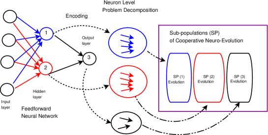
In Algorithm 1, the network is decomposed according to the selected decomposition method. Neuron level decomposition is shown in Figure 1. Once the decomposition is done, the subcomponents that are implemented as sub-populations are initialized and evolved in a round-robin fashion, typically for a fixed depth of search given by generations. The evaluation of the fitness of each individual for a particular sub-population is done cooperatively by concatenating the current individual with the fittest individuals from the rest of the sub-populations [33]. The concatenated individual is then encoded into the neural network where its fitness is evaluated and returned. Although it is a representative fitness, the fitness of the entire network is assigned to the particular individual of the sub-population. This is further illustrated in Figure 1.

Figure 1: Feedforward network with Neuron level decomposition. Note that 4 input neurons represent time series reconstruction with timespan of 4.

2.3 Dynamic programming and reinforcement learning

Dynamic programming (also known as dynamic optimisation) is a optimisation strategy that considers breaking a large problem into sub-problems and using their solution as a building block to solve the bigger problem [60]. By simply using previously computed solution taken from a sub-problem, the paradigm improves the computation time and also becomes efficient in memory or storage. Although dynamic programming has typically been an approach for optimisation and sequential problems [61], it has been well used in the areas of machine learning (such as spoken word recognition [62]), and computer vision (such as variational problems [63]).

Reinforcement learning on the other hand, considers agents that take actions in an environment to maximise the notion of cumulative reward [64]. Reinforcement learning has a wide range of multi-disciplinary applications such as game theory, control theory, and operations research [65]. In the operations research and control literature, reinforcement learning is called approximate dynamic programming [66], or neuro-dynamic programming [67]. They combine ideas from the fields of neural networks, cognitive science and approximation theory. In machine learning, the environment is typically formulated as a Markov decision process (MDP) where the outcomes are partly random and partly under the control of a decision maker. Opposed to classical dynamic programming, reinforcement learning does not assume knowledge of an exact mathematical model of the MDP. Recent application via deep learning considers learning of policies directly from high-dimensional sensory inputs in the challenging domain of classic Atari 2600 games [68].

Evolutionary algorithms have been proposed as a method for reinforcement learning [69]. Reinforcement learning via evolutionary algorithms have been implemented as neuroevolution [70] for neural networks with application for playing the game of ’Go’. Reinforcement learning more recently has been implemented with co-evolutionary algorithms in a classical control problem that considers balancing double inverted poles [52]. This further motivates the methodology presented in this paper that provides a synergy between, dynamic programming, reinforcement learning and neuroevolution for co-evolutionary multi-task learning.

2.4 Machine learning and optimisation

Essentially, machine learning algorithms have three components that include representation, evaluation and optimisation. Representation is done in the initial stage when the problem is defined and form formulated. Representation considers the type of problem (classification, regression or prediction) and the evaluation metrics such as squared error loss and classification performance. Representation also considers initialisation of the parameters, such as the weights of the neural networks and hyper parameters such as the learning rate. In the case of cooperative neuroevolution, the representation component would consider the encoding of the network weights into the subpopulations and initialising them for evolution. Evaluation and optimisation are components that iterate over time until a certain condition is met. Machine learning can also be seen as a data driven optimisation process. The learning procedure can be seen as solving a core optimisation problem that optimises the variables or parameters of the model with respect to the given loss function. Evolutionary algorithms are typically considered as optimisation methods and their synergy with neural networks into neuroevolution can be viewed as a learning procedure. In this paper, learning in neural networks is implemented using co-evolutionary algorithms that features elements from multi-task learning and dynamic programming. Moreover, learning is also referred to evolution in the context of neuroevolution. Bennett and Parrado-Hernández in an introductory note to a special issue of a journal mentioned that optimisation problems lie at the heart of most machine learning approaches [71]. They highlighted the need for dealing with uncertainty, convex models, hyper-parameters, and hybrid approaches of optimisation methods for learning. Furthermore, Guillory et al. showed that online active learning algorithms can be viewed as stochastic gradient descent on non-convex objective functions [72].

2.5 Problems in time series prediction

Although a number of methods have been used for one-step ahead prediction, neural networks have given promising results with different architectures [2, 7] and algorithms that include gradient-based learning [73, 1], evolutionary algorithms [6, 7, 8], and hybrid learning methods [3, 4, 2]. These methods can also be used for multi-step ahead and multivariate time series prediction. Multi-step-ahead (MSA) prediction refers to the forecasting or prediction of a sequence of future values from observed trend in a time series [74]. It is challenging to develop models that produce low prediction error as the prediction horizon increases [17, 18, 19]. MSA prediction has been approached mostly with the recursive and direct strategies. In the recursive strategy, the prediction from a one-step-ahead prediction model is used as input for future prediction horizon [75, 76]. Although relatively new, a third strategy is a combination of these approaches [75, 77].

Multi-variate time series prediction typically involves the prediction of single or multiple values from multi-variate input that are typically interconnected through some event [20, 21, 22]. Examples of single value prediction are the prediction of flour prices of time series obtained from different cities [20] and traffic time series [78]. The goal in this case is to enhance the prediction performance from the additional features in the input, although the problem can be solved in a univariate approach [78]. In the case of prediction of multiple values, the model needs to predict future values of the different features, for example, prediction of latitude and longitude that defines the movement of cyclones [79]. A recent study has shown that multivariate prediction would perform better than univariate for MSA as the prediction horizon becomes larger, multi-variate information becomes more important [80]. Another area of problems in time series prediction consist of applications that have missing data. Wu et al. approached the missing data problem in time series with non-linear filters and neural networks [81]. In their method, a sequence of independent Bernoulli random variables were used to model random interruptions which was later used to construct the state-space vector in pre-processing stage.

Furthermore, novel approaches that feature a synergy of different methodologies have recently been presented to address time series prediction. Extreme value analysis considers the extreme deviations from the median of probability distributions, which has been beneficial for time series prediction in the past [82]. D’Urso et al. explored the grouping of time series with similar seasonal patterns using extreme value analysis with fuzzy clustering with an application daily sea-level time series in Australia [83]. Chouikhi et al. presented echo state networks for time series prediction where particle swarm optimised was used to optimise the untrained weights that gave enhancement to learning [84]. Such approaches give motivations for developing a synergy of different methods in order to utilise their strengths and eliminate their weaknesses.

3 Co-evolutionary Multi-task Learning

3.1 Preliminaries: time series reconstruction

State-space reconstruction considers the use of Taken’s theorem which expresses that the state-space vector reproduces important characteristics of the original time series [9]. Given an observed time series $x(t)$, an embedded state space $Y(t)=[(x(t),x(t-T),...,x(t-(D-1)T)]$ can be generated, where, $T$ is the time delay, $D$ is the timespan (also known as embedding dimension), $t=(D-1)T,DT,...,N-1$, and $N$ is the length of the original time series. The optimal values for $D$ and $T$ must be chosen in order to efficiently apply Taken’s theorem [85]. Taken’s proved that if the original attractor is of dimension $d$, then $D=2d+1$ will be sufficient to reconstruct the attractor [9]. In the case of using feedforward neural networks, $D$ is the number of input neurons.

3.2 Dynamic time series prediction

Natural disasters such as torrential rainfall, cyclones, tornadoes, wave surges and droughts [86, 87, 15, 14] require dynamic and robust prediction models that can make a decision as soon as the event take place. Therefore, if the model is trained over specific months for rainy seasons, the system should be able to make a robust prediction from the beginning of the rainy season. We define the event length as the duration of an event which can be number of hours of a cyclone or number of days of drought or torrential rain.

As noted earlier, in a typical time series prediction problem, the original time series is reconstructed using Taken’s theorem [9, 85]. In the case of cyclones, it is important to measure the performance of the model when dynamic prediction is needed regarding track, wind or other characteristics of the cyclone [16]. Dynamic prediction can provide early warnings to the community at risk. For instance, data about tropical cyclone in the South Pacific is recorded at six hour intervals [88]. If the timespan $D=6$, the first prediction by the model at hand would come after 36 hours which could have devastating effects.

The problem arises when the gap between each data point in the times series is a day or number of hours. The problem with the existing models such as neural networks used for cyclones is the minimal timespan $D$ needed to make a prediction. It has been reported that recurrent neural networks trained with a given timespan (e.g. $D=5$), cannot make robust prediction for other timespan ( e.g. $D=7$ or $D=3$ ) [16]. Therefore, we introduce and define the problem of dynamic time series prediction that refers to the ability of a model to give a prediction given a set of timespan values rather than a single one. This enables the model to make decision with minimum value of the timespan in cases when rest of features of data-points are not available. A conventional one-step ahead time series prediction can be given by

$$\begin{split}\textbf{x}&=x[t],x[t-1],...,x[t-D]\\ xˆ[t+1]&=f(\textbf{x})\end{split}$$ (1)

where $f(.)$ is a model such as a feedforward neural network and $D$ is a fixed value for the timespan and x refers to the input features. In the case of dynamic time series, rather than a single value, we consider a set of values for the timespan

$$\Omega_{m}=[D_{1},D_{2},...D_{M}]$$ (2)

where $M$ is the number of subtasks, given $M\leq D$. Hence, the input features for each subtask in dynamic time series prediction can be given by $\Psi_{m}$, where $m=1,2,...,M$.

$$\begin{split}\Psi_{m}&=x[t],x[t-1],...,x[t-\Omega_{m}]\\ \end{split}$$ (3)

3.3 Method

In the proposed method, a co-evolutionary algorithm based on a dynamic programming strategy is proposed for multi-task learning. It features problem decomposition in a similar way as cooperative coevolution, however, the major difference lies in the way the solutions of the subcomponents are combined to build to the final solution. Hence, the proposed co-evolutionary multi-task learning algorithm is inspired from the strategies used in dynamic programming where a subset of the solution is used as the main building block for the optimisation problem. In this case, the problem is learning the weights of a cascaded neural network architecture where the base problem is the network module that is defined by lowest number of input features and hidden neurons.

The weights in the base network are part of larger cascaded network modules that consist of additional hidden neurons and input features. This can be viewed as modules of knowledge that are combined for larger subtasks that use knowledge from smaller subtasks as building blocks. The cascaded network architecture can also be viewed as an ensemble of neural networks that feature distinct topologies in terms of number input and hidden neurons as shown in Figure 2. Suppose that we refer to a module in the cascaded ensemble, there are $M$ modules with input $i$, hidden $h$ layers as shown.

$$\begin{split}I&=[i_{1},i_{2},...,i_{M}]\\ H&=[h_{1},h_{2},...,h_{M}]\\ O&=[1,1,...,1]\end{split}$$ (4)

where $I$, $H$, and $O$ contain the set of input, hidden and output layers. Note that the approach considers fixed number of output neurons. Since we consider one-step-ahead time series problem, one neuron in output layer is used for all the respective modules. The input for each of the modules is given by the dynamic nature of the problem that considers different lengths of timespan that constructs an input vector $\Psi_{m}$ for the given module as follows.

$$\Psi_{m}=x[t],x[t-1],...,x[t-I_{m}]$$ (5)

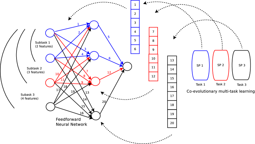
Note that the input-hidden layer $\omega_{m}$ weights and the hidden-output layer $\upsilon_{m}$ weights are combined for the respective module $m$. The base knowledge module is given as $\Phi_{1}=[\omega_{1},\upsilon_{1}]$. The subtask $\theta_{m}$ is defined as the problem of training the respective knowledge modules $\Phi_{m}$ with given input $\Psi_{m}$. Note that Figure 3 explicitly shows the knowledge modules of the network for $\omega_{2}$ and $\omega_{1}$, respectively. The knowledge module for each subtask is constructed in a cascaded network architecture as follows.

$$\Phi_{1} =[\omega_{1},\upsilon_{1}];\;\;\theta_{1}=(\Phi_{1})$$

$$\Phi_{2} =[\omega_{2},\upsilon_{2}];\;\;\theta_{2}=[\theta_{1},\Phi_{2}]$$

$$\vdots$$

$$\Phi_{M} =[\omega_{M},\upsilon_{M}];\;\;\theta_{M}=[\theta_{M-1},\Phi_{M}]$$

The vector of knowledge modules considered for training or optimisation is therefore $\mathbf{\Phi}=(\Phi_{1},\ldots,\Phi_{M})$.

$$\begin{split}y_{1}&=f(\theta_{1},\Psi_{1})\\ y_{2}&=f(\theta_{2},\Psi_{2})\\ &\vdots\\ y_{M}&=f(\theta_{M},\Psi_{M})\end{split}$$ (7)

Given $T$ samples of data, the loss $L$ for sample $t$ can be calculated by root mean squared error.

$$L_{t}=\sqrt{\frac{1}{M}\sum_{m=1}^{M}\left(\hat{y}-y_{m}\right)^{2}}$$ (8)

where $\hat{y}$ is the observed time series and $y_{m}$ is the prediction given by subtask $m$. The loss $E$ for the entire dataset (all subtasks) is given by

$$E=\frac{1}{T}\sum_{t=1}^{T}L_{t}$$ (9)

The training of the cascaded network architecture involves decomposition as subtasks through co-evolutionary multi-task learning (CMTL) algorithm. The knowledge modules in subtasks denoted by $\Phi_{m}$ are implemented as subcomponents $S_{1},S_{2},..S_{M}$, where $M$ is number of subtasks. The subcomponents are implemented as sub-populations consist of matrix of variables that feature the weights and biases $S_{m}=\Pi_{i,j}$, where $i$ refers to weights and biases and $j$ refers to the individuals. The individuals of the sub-populations are referred as genotype while the corresponding network module are referred as the phenotype. Unlike conventional transfer learning methods, the transfer of knowledge here is done implicitly through the sub-populations in CMTL. The additional subtasks are implemented through the cascades that utilise knowledge from the base subtask. The fitness of the cascade is evaluated by utilising the knowledge from the base subtask. This is done through CMTL where the best solution from the sub-population of the base subtask is concatenated with the current individual from the sub-population whose fitness needs to be evaluated. This is how transfer of knowledge is implicitly done through co-evolutionary multi-task learning.

Data: Requires input $\Psi_{m}$ taken from data $\Sigma$ for respective subtasks $\theta_{m}$.

Result: Prediction error $E$ for dynamic time series

for each module $m$ do

       1. Assign fixed depth of search $\beta$ that defines the number of generation of evolution for each subcomponent $S_{m}$; (eg. $\beta=5$ ) 2. Define the weight space (input - hidden and hidden - output layer) for the different subtasks $\theta_{m}$ defined by the respective network module $\Phi_{m}=[\omega_{m},\upsilon_{m}]$.  3. Create $X_{m}$ vector of subtask solutions from $\Theta_{m}$. Note that the size of $X_{m}$ depends on number of network module considered in the subtask. 4. Initialise genotype of the sub-populations $S_{m_{j}}$ given by $j$ individuals in a range $[-\alpha,\alpha]$ drawn from a uniform distribution where $\alpha$ defines the range.

end while each phase until termination do

       for each subtask $m$ do

             for each generation until $\beta$ do

                   for each Individual $j$ in subpopulation $\Pi_{i,j}$ do

                         ** Stage 1:
* Assign $B_{m}$ as best individual for subtask $m$ from subpopulation $\Pi_{i,j}$
if $m==1$ then

                               * Get the current individual from subpopulation; $V_{1}=\Pi_{i,j}$ where $i$ includes all the variables (weights). Assign the current individual as $X_{1}=V_{1}$

                        end else

                               * Get the current individual from subpopulation; $V_{m}=\Pi_{i,j}$. Append the current subtask solution with best solutions from previous subtasks, $X_{m}=[B_{1},...,B_{m-1},V_{m}]$ where $B$ is the best individual from previous subtask and $V$ is the current individual that needs to be evaluated.

                        end ** Stage 2:
* Execute Algorithm 3: This will encode the $X_{m}$ into knowledge modules $\Phi=(\Phi_{1},\ldots,\Phi_{M})$ for subtasks $f(\theta_{m},\Psi_{m})$ * Calculate subtask output $y_{m}=f(\theta_{m},\Psi_{m})$ and evaluate the given genotype though the loss function $E=\frac{1}{T}\sum_{t=1}^{T}L_{t}$, where $L_{t}$ is given in Equation 9.

                  end for each Individual $j$ in $S_{m}$ do

                         * Create new offspring via evolutionary operators such selection, crossover and mutation

                  end * Update $S_{m}$  

            end

      end

end * Test the obtained solution for each module $m$ do

       1. Load best solution $S_{best}$ from $S_{m}$.   2. Encode into the respective weight space for the subtask $\Phi_{m}=[\omega_{m},\upsilon_{m}]$.  3. Calculate loss $E$ based on the test dataset.

end

Algorithm 2 Co-evolutionary multi-task learning

Algorithm 2 gives details for CMTL which begins by initialising the the sub-populations defined by the subtasks which feature the knowledge modules $\Phi_{m}$ and respective subtask input features $\Psi_{m}$. The sub-populations are initialised with real values $[-\alpha,\alpha]$ drawn from uniform distribution where $\alpha$ defines the range. Once this has been done, the algorithm moves into the evolution phase where each subtask is evolved for a fixed number for generations defined by depth of search, $\beta$. The major concern here is the way the phenotype is mapped into genotype where a group of weight matrices given by $\Phi_{m}=[\omega_{m},\upsilon_{m}]$ that makes up subtask $\theta_{m}$ are converted into vector $X_{m}$. Stage 1 in Algorithm 2 implements the use of knowledge from previous subtasks through multi-task learning. In the case if the subtask is a base problem ($m==1$), then the subtask solution $X_{m}$ is utilised in a conventional matter where knowledge from other subtasks or modules are not required to reach a decision. Howsoever, given that the subtask is not a base problem, the current subtask individual $X_{m}$ is appended with best individuals from the previous subtasks, therefore, $X_{m}=[B_{1},...,B_{m-1},V_{m}]$, where $B$ is the best individual from previous subtask and $V$ is the current individual that needs to be evaluated. This will encode $X_{m}$ into knowledge modules $\mathbf{\Phi}=(\Phi_{1},\ldots,\Phi_{M})$ for the respective subtasks. The algorithm then calculates subtask network output or prediction $y_{m}=f(\theta_{m},\Psi_{m})$ and evaluate the individual though the loss function $E=\frac{1}{T}\sum_{t=1}^{T}L_{t}$, where $L_{t}$ is given in Equation 9. The subtask solution is passed to Algorithm 3 along with the network topology in order to decode the subtask solution into the respective weights of the network. This could be seen as the process of genotype to phenotype mapping. This procedure is executed for every individual in the sub-population. This procedure is repeated for every sub-population for different phases until the termination condition is satisfied. The termination condition can be either the maximum number of function evaluations or a minimum fitness value from the training or validation dataset. Figure 2 shows an exploded view of the neural network topologies associated with the respective subtasks, however, they are part of the cascaded network architecture later shown in Figure 3. The way the subtask solution is decomposed and mapped into the network is given in Figure 3 and discussed detail in the next section.

The major difference in the implementation of CMTL when compared to conventional cooperative neuroevolution (Algorithm 1) is by the way the problem is decomposed and the way the fitness for each individual is calculated. CMTL is motivated by dynamic programming approach where the best solution from previous sub-populations are used for cooperative fitness evaluation for individuals in the current sub-population. Howsoever, the current sub-population does not use the best solution from future subpopulations. This way, the concept of utilising knowledge from previous subtasks as building blocks is implemented . On the other hand, cooperative neuroevolution follows a divide and conquer approach where at any given subpopulation, in order to evaluate the individuals, the best individuals from the rest of the sub-populations are taken into account.

Figure 2: Problem decomposition as subtasks in co-evolutionary multi-task learning. Note that the colours associated with the synapses in the network are linked to their encoding that are given as different subtasks. Subtask 1 employs a network topology with 2 hidden neurons while the rest of the subtasks add extra input and hidden neurons. The exploded view shows that the different neural network topologies are assigned to the different subtasks, however, they are all part of the same network as shown in Figure 3

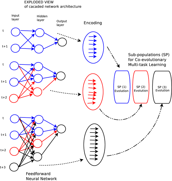
Finally, when the termination criteria has been met, the algorithm moves into the testing phase where the best solutions from all the different subtasks are saved and encoded into their respective network topologies. Once this is done, the respective subtask test data is loaded and the network makes prediction that is evaluated with loss $E$ given in Equation 9. Other measure of error can also be implemented. Hence, we have highlighted the association of every individual in the respective sub-populations with different subtasks in the multi-task learning environment. There is transfer of knowledge in terms of weights from smaller to bigger networks as defined by the subtask with its data which is covered in detail in next section. A Matlab implementation of this algorithm with respective datasets used for the experiments is given online .

3.4 Transfer of knowledge

One challenging aspect of the Algorithm 2 is the transfer of knowledge represented by the weights of the respective neural networks that is learnt by the different subtasks in CMTL. The cascading network architecture increase in terms of the input and hidden neurons with the subtasks. Algorithm 3 implements transfer of knowledge given the changes of the architecture by the different subtasks. The goal is to transfer weights that are mapped from different sub-populations defined by the subtasks. The algorithm is given input parameters which are

1. The reference to subtask $m$;

2. The current subtask solution; if $m$ is base task, $X_{m}=[V_{m}]$ else $X_{m}=[B_{1},...,B_{m-1},V_{m}]$, otherwise.

3. The topology of the respective cascaded neural module for the different subtasks in terms of number of input, hidden, and output neurons.

We describe the algorithm with reference to Figure 3 which shows a case, where the subtask $m=3$ goes through the transfer where $m=1$ and $m=2$ are used as building blocks of knowledge given in the weights. Therefore, we use examples for the network topology as highlighted below.

1. $I_{m}$ is vector of number of input neurons for the respective subtasks, eg. $I=[2,3,4]$ ;

2. $H_{m}$ is vector of number of input neurons for the respective subtasks, eg. $H_{=}[2,3,4]$;

3. $O_{m}$ is vector of output neurons for the respective subtasks, eg. $O=[1,1,1]$.

The algorithm begins by assigning base case, $b=1$ which is applied irrespective of the number of subtasks. In Step 1, the transfer of Input-Hidden layer weights is shown by weights (1-4) in Figure 3. Step 2 executes the transfer for Hidden-Output layer weights as shown by weights (5-6) in Figure 3. Note that Step 1 and 2 are applied for all the cases given by the number of subtasks. Once this is done, the algorithm terminates if $m=1$ or proceeds if $m>=2$. Moving on, in Step 3, the case is more complex as we consider $m>=2$. Step 1 and 2 are executed before moving to Step 3 where $X$ contains the appended solution sets from previous subtasks. In Step 3, $t$ in principle points to the beginning of the solution given by sub-population for $m=2$. Here, the transfer for Input-Hidden layer weights (7-9) is executed for $m=2$. Note that in this case, we begin with the weights with reference to the number of hidden neurons from previous subtask $j=H_{(m-1)}+1$, and move to the number of hidden neurons of the current subtask $j=H_{(m)}$ in order to transfer the weights to all the input neurons. This refers to weights (7-9) in Figure 3. Before reaching transfer for $m=3$, $m=1$ and $m=2$ transfer would have already taken place and hence the weights (13-16) would be transferred as shown in the same figure. Moving on to Step 4, we first consider the transfer for Input-Hidden layer weights for $m=2$ through the transfer of weights from beginning of previous subtask input, $i=I_{(m-1)}+1$ to current subtask input connected with all hidden neurons. This is given by weights (10-11) in Figure 3. For the case of $m=3$, this would refer to weights (17-19) in the same figure.

Finally, in Step 5, the algorithm executes the transfer for Hidden-Output layer weights based on the hidden neurons from previous subtask. In case of $m=2$, this results in transferring weight (12) and for $m=3$, the transfer is weight (20) in Figure 3, respectively. Note that the algorithm can transfer any number of input and hidden neurons as the number of subtasks increase.

Parameters: Subtask $m$, module subtask solution $X$ , Input $I$, Hidden $H$ and Output $O$

$b=1$; ( Base task)

Step 1

for each $j=1$ to $H_{b}$ do

       for each $i=1$ to $I_{b}$ do

             $W_{ij}=X_{t}$  
$t=t+1$  

      end

end Step 2 for each $k=1$ to $O_{b}$ do

       for each $j=1$ to $H_{b}$ do

             $W_{jk}=X_{t}$  
$t=t+1$  

      end

end if m $>=$ 2 then

       Step 3 for each $j=H_{m-1}+1$ to $H_{m}$ do

             for each $i=1$ to $I_{m}$ do

                   $W_{ij}=X_{t}$  
$t=t+1$  

            end

      end Step 4 for each $j=1$ to $H_{m}$ -1 do

             for each $i=I_{m-1}+1$ to $I_{m}$ do

                   $W_{ij}=X_{t}$  
$t=t+1$  

            end

      end Step 5 for each $k=1$ to $O_{m}$ do

             for each $j=H_{m-1}+1$ to $H_{m}$ do

                   $W_{j,k}=X_{t}$  
$t=t+1$  

            end

      end

end

Algorithm 3 Transfer of knowledge from previous subtasks

Figure 3: Transfer of knowledge from subtasks encoding as sub-populations in co-evolutionary multi-task learning algorithm. This diagram shows transfer of knowledge from Subtask 1 and Subtask 2. Once the knowledge is transferred into Subtask 3, the network loads Subtask 3 dataset (4 features in this example) for further evolution of the related sub-population

The time complexity of CMTL considers the time taken for transfer of solutions for different number of subtasks. We note that the best case is when the subtask is the base subtask $(m=1)$. Therefore, the worst case time complexity can be given by

$$\begin{split}T(m<=1)&=O(1)\\ T(m)&=T(m-1)+T(m-2),...,+O(1)\\ T(m)&=O(2^{m})\end{split}$$ (10)

where $m$ refers to the subtasks.

4 Simulation and Analysis

This section presents an experimental study that compares the performance of CMTL with conventional neuroevolution methods. The results are compared with neuroevolution via evolutionary algorithm (EA) and cooperative neuroevolution (CNE) for benchmark time series prediction problems. Furthermore, tropical cyclones from South Pacific and South Indian Ocean are considered to address the minimal timespan issue [16] using dynamic time series prediction.

4.1 Benchmark Chaotic Time Series Problems

In the benchmark chaotic time series problems, the Mackey-Glass, Lorenz, Henon and Rossler are the four synthetic time series problems. The experiments use the chaotic time series with length of 1000 generated by the respective chaotic attractor. The first 500 samples are used for training and the remaining for testing.

In all cases, the phase space of the original time series is reconstructed with the timespan for 3 datasets for the respective subtasks with the set of timespan $\Omega=[3,5,7]$ and time lag $T=2$. All the synthetic and real-world time series were scaled in the range [0,1]. Further details of each of the time series problem is given as follows.

The Mackey-Glass time series has been used in literature as a benchmark problem due to its chaotic nature [89]. The Lorenz time series was introduced by Edward Lorenz who has extensively contributed to the establishment of Chaos theory [90]. The Henon time series is generated with a Henon map which is a discrete-time dynamical system that exhibit chaotic behaviour [91] and the Rossler time series is generated using the attractor for the Rossler system, a system of three non-linear ordinary differential equations as given in [92]. The real-world problem are the Sunspot, ACI finance and Laser time series. The Sunspot time series is a good indication of the solar activities for solar cycles which impacts Earth’s climate, weather patterns, satellite and space missions [93]. The Sunspot time series from November 1834 to June 2001 is selected which consists of 2000 points. The ACI financial time series is obtained from the ACI Worldwide Inc. which is one of the companies listed on the NASDAQ stock exchange. The data set contains closing stock prices from December 2006 to February 2010, which is equivalent to approximately 800 data points. The closing stock prices were normalised between 0 and 1. The data set features the recession that hit the U.S. market in 2008 [94]. The Laser time series is measured in a physics laboratory experiment that were used in the Santa Fe Competition [95]. All the real world time series used the first 50 percent samples for training and remaining for testing.

4.2 Cyclone time series

The Southern Hemisphere tropical cyclone best-track data from Joint Typhoon Warning Centre recorded every 6-hours is used as the main source of data [88]. We consider only the austral summer tropical cyclone season (November to April) from 1985 to 2013 data in the current study as data prior to the satellite era is not reliable due to inconsistencies and missing values. The original data of tropical cyclone wind intensity in the South Pacific was divided into training and testing set as follows:

• Training Set: Cyclones from 1985 - 2005 (219 Cyclones with 6837 data points)

• Testing Set: Cyclones from 2006 - 2013 (71 Cyclones with 2600 data points)

In the case for South Indian Ocean, the details are as follows:

• Training Set: Cyclones from 1985 - 2001 ( 285 Cyclones with 9365 data points)

• Testing Set: Cyclones from 2002 - 2013 ( 190 Cyclones with 8295 data points )

Although the cyclones are separate events, we choose to combine all the cyclone data in a consecutive order as given by their date of occurrence. The time series is reconstructed with the set of timespan, $\Omega=[3,5,7]$, and time lag $T=2$.

4.3 Experimental Design

We note that multi-task learning approach used for dynamic time series can be formulated as a series of independent single task learning approaches. Hence, for comparison of CMTL, we provide experimentation and results with conventional neuroevolution methods that can be considered as single-task learning (CNE and EA). In the case of CNE, neuron level problem decomposition is applied for training feedforward networks [55]. We employ covariance matrix adaptation evolution strategies (CMAES) [96] as the evolutionary algorithm in sub-populations of CMTL, CNE and the population of EA. The training and generalisation performances are reported for each case given by the different subtasks in the respective time series problems.

The respective neural networks used both sigmoid units in the hidden and output layer for all the different problems. The loss function given in Equation 9 is used as the main performance measure. Each neural network architecture was tested with different numbers of hidden neurons.

We employ fixed $depth=5$ generation in the sub-populations of CMTL as the depth of search as it has given optimal performance in trial runs. CNE also employs the same value. Note that all the sub-populations evolve for the same depth of search. The population size of CMAES in the respective methods is given by $P=4+floor*(3*log(W))$, where $W$ is the total number of weights and biases for the entire neural network that includes all the subtasks (CMTL). In the case of EA and CNE, $W$ is total number of weights and biases for the given network architecture.

The termination condition is fixed at 30 000 function evaluations for each subtask, hence, CMTL employs 120 000 function evaluations while conventional methods use 30 000 for each of the respective subtasks for all the problems. Note that since there is a fixed training time, there was no validation set used to stop training. The choice of the parameters such as the appropriate population size, termination condition has been determined in trial experiments. The experiments are well aligned with experimental setting from previous work [7, 97].

4.4 Results for Benchmark Problems

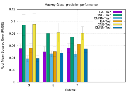
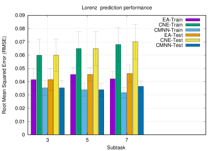
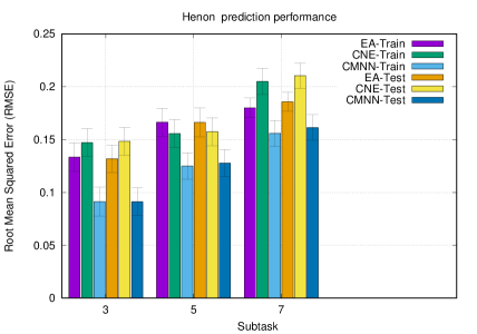
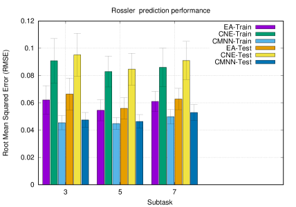
The results for the 7 benchmark chaotic time series problems are given in Figure 4 to 10 which highlight the training and generalisation performance. We limit our discussion to the generalisation performance, although the training performance is also shown. Figure 4 shows that CMTL generalisation performance is better than EA and CNE, while CMTL and EA outperform CNE in all the subtasks denoted by the timespan. The same trend is shown in general for Lorenz and Henon time series as shown in Figure 5 and Figure 6, respectively. There is one exception ($D=5$), for the Henon problem where CME gives better performance than EA, however, worse than CMTL. Figure 7 shows the results for the Rossler time series which follows a similar trend when compared to the previous problems. Hence, in general, CMTL generalisation performance is the best when compared to the conventional methods (CNE and EA) for the 4 synthetic time series problems which have little or no noise present.

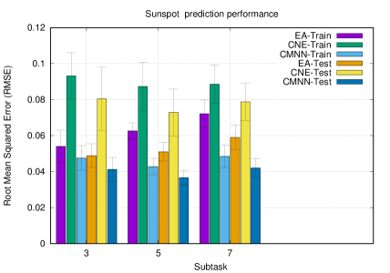
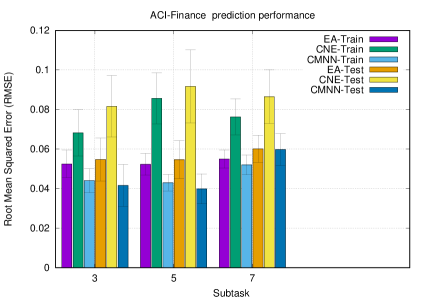
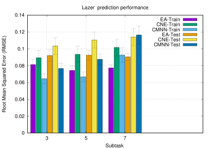
In the case of real-world problems, Figure 8 for the Sunspot problem shows that CMTL provides the best generalisation performance when compared to EA and CNE for all the cases. The same is given for first two timespan cases for ACI-finance problem as shown in Figure 9, except for one case ($D=7$), where EA and CMTL gives the same performance. In the case of the Laser time series in Figure 10, which is known as one of the most chaotic time series problems, CMTL outperforms CNE and EA, except for one case, $D=7$. Therefore, at this stage, we can conclude that CMTL gives the best performance for most of the cases in the real-world time series problems. Table 1 shows the mean of RMSE and confidence interval across the 3 timespan. We find that the CMTL performs better than EA and CNE for almost all the problems. The Laser problem is the only exception where the EA is slightly better than CMTL.

Figure 4: Performance given by EA, CNE, CMTL for Mackey-Glass time series

Figure 5: Performance given by EA, CNE, CMTL for Lorenz time series

Figure 6: Performance given by EA, CNE, CMTL for Henon time series

Figure 7: Performance given by EA, CNE, CMTL for Rossler time series

Figure 8: Performance given by EA, CNE, CMTL for Sunspot time series

Figure 9: Performance given by EA, CNE, CMTL for ACI-finance time series

Figure 10: Performance given by EA, CNE, CMTL for Laser time series

Table 1: Combined mean prediction performance for 3 subtasks

Problem	EA	CNE	CMTL
Mackey-Glass	0.0564 $\pm$0.0081	0.0859 $\pm$0.0147	0.0472 $\pm$0.0054
Lorenz	0.0444 $\pm$0.0067	0.0650 $\pm$ 0.0127	0.0353 $\pm$ 0.0049
Henon	0.1612 $\pm$ 0.0120	0.1721 $\pm$ 0.0128	0.1267 0.0127
Rossler	0.0617$\pm$ 0.0091	0.0903$\pm$ 0.0138	0.0489 $\pm$0.0054
Sunspot	0.0529 $\pm$ 0.0062	0.0773 $\pm$0.0137	0.0399 $\pm$ 0.0052
Lazer	0.0917 $\pm$0.0056	0.1093 $\pm$0.0099	0.0936 $\pm$0.0077
ACI-finance	0.0565 $\pm$0.0091	0.0866 $\pm$0.0159	0.0471 $\pm$0.0087

4.5 Results for Tropical Cyclones

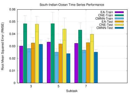
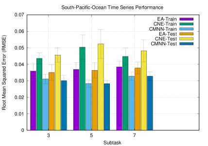
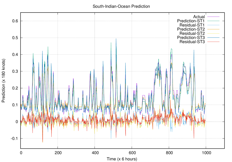
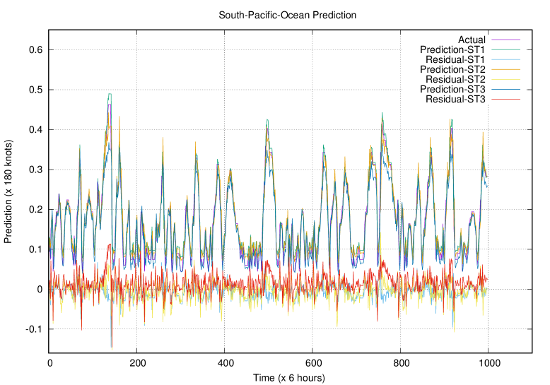
We present the results for the performance of the given methods on the two selected cyclone problems, which features South Pacific and South Indian ocean as shown in Figure 11 and Figure 12, respectively. Figures 14 and 13 show the prediction performance of a typical experimental run. In the case of the South Pacific ocean, the results show that CMTL provides the best generalisation performance when compared to CNE and EA. This is also observed for the South Indian ocean.

Figure 11: Performance given by EA, CNE, CMTL for South Indian ocean

Figure 12: Performance given by EA, CNE, CMTL for South Pacific ocean

Figure 13: Typical prediction performance given by different CMTL subtasks (ST1, ST2, and ST3) for the South Indian ocean

Figure 14: Typical prediction performance given by different CMTL subtasks (ST1, ST2, and ST3) for the South Pacific ocean

4.6 Discussion

The goal of the experiments was to evaluate if CMTL can maintain quality in prediction performance when compared to conventional methods, while at the same time address dynamic time series problems. The results have shown that CMTL not only addresses dynamic time series but is a way to improve the performance if each of the subtasks in multi-task learning was decomposed and approached as single-task learning. The incremental learning in CMTL not only improves the prediction performance but also ensures modularity in the organisation of knowledge. Modularity is an important attribute for addressing dynamic prediction problems since groups of knowledge can be combined to make a decision when the nature or complexity of the problem increases. Modularity is important for design of neural network in hardware [98] as disruptions in certain synapse(s) can result in problems with the whole network which can be eliminated by persevering knowledge as modules [28].

It is noteworthy that CMTL gives consistent performance even for the cases when the problem is harder as in the case of smaller or foundational subtasks that have minimal timespan. Learning smaller networks could be harder since they have limited information about the past behaviour of the time series. The way the algorithm handles this issue is with the refinement of the solutions (in a round-robin manner through coevolution) after it has been transferred to a larger network. When more information is presented as the subtask increases, CMTL tends to refine the knowledge in the smaller subtasks. In this way, the results show that the performance is consistent given the small subtasks and when they increase depending on the timespan.

CMTL can be seen as a flexible method for datasets that have different features of which some have properties so that they can be grouped together as subtasks. Through multi-task learning, the overlapping features can be used as building blocks to learn the nature of the problem through the model at hand. Although feedforward neural networks have been used in CMTL, other other neural network architectures and learning models can be used depending on the nature of the subtasks. In case of computer vision applications such as face recognition, the different subtasks can be different number of features; i.e. the algorithm can execute face recognition based on minimal features from a set of features.

CMTL could also be viewed as training cascaded networks using a dynamic programming approach where each cascade defines a subtask. Although the depth of the cascading does not have a limit, adding cascades could result in an exponential increase of training time. The depth of the cascaded architecture would be dependent on the application problem. It depends on the time series under consideration and the level of inter-dependencies of the current and the previous time steps. In principle, one should stop adding cascades when the prediction performance begins to deteriorate to a given threshold. Therefore, for a given problem, there needs to be systematic approach that selects the number of subtasks for the cascaded architecture.

We have experimentally tested robustness and scalability using the synthetic and real-world datasets that includes benchmark problems and an application that considers the prediction of wind-intensity in tropical cyclones. We provided comprehensive experimentation for the algorithm convergence given a range of initial conditions. These include different set of initialisation of the subpopulations in CMTL with multiple experimental runs along with further reporting of the mean and confidence interval. We evaluated the prediction capability given different instances of the timespan defined as subtasks in CMTL and compared the performance with standalone methods. The experimental design considered multiples experiment runs, different and distinct datasets, difference in size of the datasets, and different sets of initialisation in the subpopulations. In this way, we have addressed robustness and convergence of the proposed method, experimentally.

In the comparison of CMTL with CNE, we observed that CMTL creates a higher time complexity since it has an additional step of transfer of solutions from the different subtasks encoded in the subpopulations. The time taken would increase exponentially as the number of subtasks increases. This would add to cost of utilising solutions from other subtasks given a fixed convergence criteria defined by the number of function evaluations. In case if the convergence criteria is defined by a minimum error or loss, it is likely that the solutions from the previous subtasks will help in faster convergence. In terms of scalability, we note that neuroevolution methods have limitations due to slow convergence of evolutionary algorithms. With help of gradient-based local search methods, convergence of CMTL can be improved via memetic algorithms where local refinement occurs during the evolution [99]. There is scope in future work convergence proof used in standard evolutionary algorithms [100] that could further be extended for multiple sub-populations in CMTL.

5 Conclusions and Future Work

We presented a novel algorithm that provides a synergy between coevolutionary algorithms and multi-tasking for dynamic time series problems. CMTL can be used to train a model that can handle multiple timespan values that defines dynamic input features which provides dynamic prediction. CMTL has been very beneficial for tropical cyclones where timely prediction needs to be made as soon as the event takes place. The results show that CMTL addresses the problem of dynamic time series and provides a robust way to improve the performance when compared to related methods.

It is important to understand how CMTL achieved better results for when compared to related methods given the same neural network topology and data for respective subtasks. CMTL can be seen as an incremental evolutionary learning method that features subtasks as building blocks of knowledge. The larger subtasks take advantage of knowledge gained from learning the smaller subtasks. Hence, there is diversity in incremental knowledge development from the base subtask which seems to be beneficial for future subtasks. However, the reason why the base subtask produces better results when compared to conventional learning can be explored with further analysis during learning. The larger subtasks with overlapping features covers the base subtask in a cascaded manner. Therefore, larger subtasks can be seen as those that have additional features that guide larger network with more hidden neurons during training.

Finally, CMTL is a novel approach that provides synergy of a wide range of fundamental methods that include, dynamic programming, reinforcement learning, multi-task learning, co-evolutionary algorithms and neuro-evolution. This makes the CMTL useful for some of the applications where the mentioned fundamental methods have been successful. Since reinforcement learning has been utilised in deep learning, the notion of reuse of knowledge as building bocks by CMTL could be applicable in areas of deep learning. In future work, apart from feed-forward networks, the idea of dynamic time series prediction that employs transfer and multi-task learning could be extended to other other areas that have simpler model representation, such as autoregressive models. Furthermore, CMTL can be used for other problems that can be broken into multiple subtasks, such as multiple step ahead and multivariate time series prediction. Although the paper explored timespan for univariate time series, the approach could be extended to pattern classification problems that involves large scale features. It can be extended for heterogeneous pattern classification problems where the dataset contains samples that have missing values or features. CMTL can also be extended for transfer learning problems that can include both heterogeneous and homogeneous domain adaptation cases. In case of tropical cyclones, a multivariate approach can be taken where the different subtasks can be seen as features that include cyclone tracks, seas surface temperature, and humidity.

References

- [1] D. Mirikitani and N. Nikolaev, “Recursive bayesian recurrent neural networks for time-series modeling,” Neural Networks, IEEE Transactions on, vol. 21, no. 2, pp. 262 –274, Feb. 2010.
- [2] M. Ardalani-Farsa and S. Zolfaghari, “Chaotic time series prediction with residual analysis method using hybrid Elman-NARX neural networks,” Neurocomputing, vol. 73, no. 13-15, pp. 2540 – 2553, 2010.
- [3] K. K. Teo, L. Wang, and Z. Lin, “Wavelet packet multi-layer perceptron for chaotic time series prediction: Effects of weight initialization,” in Proceedings of the International Conference on Computational Science-Part II, ser. ICCS ’01, 2001, pp. 310–317.
- [4] A. Gholipour, B. N. Araabi, and C. Lucas, “Predicting chaotic time series using neural and neurofuzzy models: A comparative study,” Neural Process. Lett., vol. 24, pp. 217–239, 2006.
- [5] D. Ruta and B. Gabrys, “Neural network ensembles for time series prediction,” in 2007 International Joint Conference on Neural Networks, 2007, pp. 1204–1209.
- [6] C.-J. Lin, C.-H. Chen, and C.-T. Lin, “A hybrid of cooperative particle swarm optimization and cultural algorithm for neural fuzzy networks and its prediction applications,” Systems, Man, and Cybernetics, Part C: Applications and Reviews, IEEE Transactions on, vol. 39, no. 1, pp. 55–68, Jan. 2009.
- [7] R. Chandra and M. Zhang, “Cooperative coevolution of Elman recurrent neural networks for chaotic time series prediction,” Neurocomputing, vol. 186, pp. 116 – 123, 2012.
- [8] R. Chandra, “Competition and collaboration in cooperative coevolution of Elman recurrent neural networks for time-series prediction,” Neural Networks and Learning Systems, IEEE Transactions on, vol. 26, pp. 3123–3136, 2015.
- [9] F. Takens, “Detecting strange attractors in turbulence,” in Dynamical Systems and Turbulence, Warwick 1980, ser. Lecture Notes in Mathematics, 1981, pp. 366–381.
- [10] R. Nand and R. Chandra, “Coevolutionary feature selection and reconstruction in neuro-evolution for time series prediction,” in Artificial Life and Computational Intelligence - Second Australasian Conference, ACALCI 2016, Canberra, ACT, Australia, February 2-5, 2016, Proceedings, 2016, pp. 285–297.
- [11] S. Chand and R. Chandra, “Multi-objective cooperative coevolution of neural networks for time series prediction,” in International Joint Conference on Neural Networks (IJCNN), Beijing, China, July 2014, pp. 190–197.
- [12] A. Maus and J. Sprott, “Neural network method for determining embedding dimension of a time series,” Communications in Nonlinear Science and Numerical Simulation, vol. 16, no. 8, pp. 3294 – 3302, 2011.
- [13] M. M. Ali, P. S. V. Jagadeesh, I. I. Lin, and J. Y. Hsu, “A neural network approach to estimate tropical cyclone heat potential in the indian ocean,” IEEE Geoscience and Remote Sensing Letters, vol. 9, no. 6, pp. 1114–1117, Nov 2012.
- [14] L. Zjavka, “Numerical weather prediction revisions using the locally trained differential polynomial network,” Expert Systems with Applications, vol. 44, pp. 265 – 274, 2016.
- [15] B. W. Stiles, R. E. Danielson, W. L. Poulsen, M. J. Brennan, S. Hristova-Veleva, T. P. Shen, and A. G. Fore, “Optimized tropical cyclone winds from quikscat: A neural network approach,” IEEE Transactions on Geoscience and Remote Sensing, vol. 52, no. 11, pp. 7418–7434, Nov 2014.
- [16] R. Deo and R. Chandra, “Identification of minimal timespan problem for recurrent neural networks with application to cyclone wind-intensity prediction,” in International Joint Conference on Neural Networks (IJCNN), Vancouver, Canada, July 2016, p. In Press.
- [17] S. B. Taieb and A. F. Atiya, “A bias and variance analysis for multistep-ahead time series forecasting,” 2015.
- [18] L.-C. Chang, P.-A. Chen, and F.-J. Chang, “Reinforced two-step-ahead weight adjustment technique for online training of recurrent neural networks,” Neural Networks and Learning Systems, IEEE Transactions on, vol. 23, no. 8, pp. 1269–1278, 2012.
- [19] R. Boné and M. Crucianu, “Multi-step-ahead prediction with neural networks: a review,” 9emes rencontres internationales: Approches Connexionnistes en Sciences, vol. 2, pp. 97–106, 2002.
- [20] K. Chakraborty, K. Mehrotra, C. K. Mohan, and S. Ranka, “Forecasting the behavior of multivariate time series using neural networks,” Neural Networks, vol. 5, no. 6, pp. 961 – 970, 1992.
- [21] L. Wang, Z. Wang, and S. Liu, “An effective multivariate time series classification approach using echo state network and adaptive differential evolution algorithm,” Expert Systems with Applications, vol. 43, pp. 237 – 249, 2016.
- [22] S. Zhang, “Adaptive spectral estimation for nonstationary multivariate time series,” Computational Statistics and Data Analysis, vol. 103, pp. 330 – 349, 2016.
- [23] R. Caruana, “Multitask learning,” Machine Learning, vol. 28, no. 1, pp. 41–75, Jul. 1997.
- [24] T. Evgeniou, C. A. Micchelli, and M. Pontil, “Learning multiple tasks with kernel methods,” Journal of Machine Learning Research, vol. 6, no. Apr, pp. 615–637, 2005.
- [25] H. Zheng, X. Geng, D. Tao, and Z. Jin, “A multi-task model for simultaneous face identification and facial expression recognition,” Neurocomputing, vol. 171, pp. 515 – 523, 2016.
- [26] T. Zeng and S. Ji, “Deep convolutional neural networks for multi-instance multi-task learning,” in Data Mining (ICDM), 2015 IEEE International Conference on, Nov 2015, pp. 579–588.
- [27] B. L. Happel and J. M. Murre, “Design and evolution of modular neural network architectures,” Neural Networks, vol. 7, no. 6–7, pp. 985 – 1004, 1994, models of Neurodynamics and Behavior. [Online]. Available: http://www.sciencedirect.com/science/article/pii/S0893608005801558
- [28] J. Clune, J.-B. Mouret, and H. Lipson, “The evolutionary origins of modularity,” Proceedings of the Royal Society of London B: Biological Sciences, vol. 280, no. 1755, 2013.
- [29] K. O. Ellefsen, J.-B. Mouret, and J. Clune, “Neural modularity helps organisms evolve to learn new skills without forgetting old skills,” PLoS Comput Biol, vol. 11, no. 4, pp. 1–24, 04 2015.
- [30] J. N. Tsitsiklis and B. V. Roy, “Neuro-dynamic programming overview and a case study in optimal stopping,” in Decision and Control, 1997., Proceedings of the 36th IEEE Conference on, vol. 2, Dec 1997, pp. 1181–1186 vol.2.
- [31] X. Fang, D. Zheng, H. He, and Z. Ni, “Data-driven heuristic dynamic programming with virtual reality,” Neurocomputing, vol. 166, pp. 244 – 255, 2015.
- [32] M. Potter and K. De Jong, “A cooperative coevolutionary approach to function optimization,” in Parallel Problem Solving from Nature — PPSN III, ser. Lecture Notes in Computer Science, Y. Davidor, H.-P. Schwefel, and R. Männer, Eds. Springer Berlin Heidelberg, 1994, vol. 866, pp. 249–257.
- [33] M. A. Potter and K. A. De Jong, “Cooperative coevolution: An architecture for evolving coadapted subcomponents,” Evol. Comput., vol. 8, pp. 1–29, 2000.
- [34] A. Gupta, Y. S. Ong, and L. Feng, “Multifactorial evolution: Toward evolutionary multitasking,” IEEE Trans. Evolutionary Computation, vol. 20, no. 3, pp. 343–357, 2016.
- [35] Y. S. Ong and A. Gupta, “Evolutionary multitasking: A computer science view of cognitive multitasking,” Cognitive Computation, vol. 8, no. 2, pp. 125–142, 2016.
- [36] R. Chandra, A. Gupta, Y. S. Ong, and C. K. Goh, “Evolutionary multi-task learning for modular knowledge representation in neural networks,” Neural Processing Letters, 2018. [Online]. Available: https://doi.org/10.1007/s11063-017-9718-z
- [37] R. Chandra, “Dynamic cyclone wind-intensity prediction using co-evolutionary multi-task learning,” in Neural Information Processing, D. Liu, S. Xie, Y. Li, D. Zhao, and E.-S. M. El-Alfy, Eds., 2017, pp. 618–627.
- [38] R. K. Ando and T. Zhang, “A framework for learning predictive structures from multiple tasks and unlabeled data,” J. Mach. Learn. Res., vol. 6, pp. 1817–1853, Dec. 2005. [Online]. Available: http://dl.acm.org/citation.cfm?id=1046920.1194905
- [39] L. Jacob, J. philippe Vert, and F. R. Bach, “Clustered multi-task learning: A convex formulation,” in Advances in Neural Information Processing Systems 21, D. Koller, D. Schuurmans, Y. Bengio, and L. Bottou, Eds. Curran Associates, Inc., 2009, pp. 745–752. [Online]. Available: http://papers.nips.cc/paper/3499-clustered-multi-task-learning-a-convex-formulation.pdf
- [40] J. Chen, L. Tang, J. Liu, and J. Ye, “A convex formulation for learning shared structures from multiple tasks,” in Proceedings of the 26th Annual International Conference on Machine Learning, ser. ICML ’09. New York, NY, USA: ACM, 2009, pp. 137–144. [Online]. Available: http://doi.acm.org/10.1145/1553374.1553392
- [41] J. Zhou, J. Chen, and J. Ye, “Clustered multi-task learning via alternating structure optimization,” in Advances in Neural Information Processing Systems 24, J. Shawe-Taylor, R. S. Zemel, P. L. Bartlett, F. Pereira, and K. Q. Weinberger, Eds. Curran Associates, Inc., 2011, pp. 702–710. [Online]. Available: http://papers.nips.cc/paper/4292-clustered-multi-task-learning-via-alternating-structure-optimization.pdf
- [42] Y. Zhang and D.-Y. Yeung, “Transfer metric learning by learning task relationships,” in Proceedings of the 16th ACM SIGKDD International Conference on Knowledge Discovery and Data Mining, ser. KDD ’10. New York, NY, USA: ACM, 2010, pp. 1199–1208. [Online]. Available: http://doi.acm.org/10.1145/1835804.1835954
- [43] B. Bakker and T. Heskes, “Task clustering and gating for bayesian multitask learning,” J. Mach. Learn. Res., vol. 4, pp. 83–99, Dec. 2003. [Online]. Available: http://dx.doi.org/10.1162/153244304322765658
- [44] S. Zhong, J. Pu, Y.-G. Jiang, R. Feng, and X. Xue, “Flexible multi-task learning with latent task grouping,” Neurocomputing, vol. 189, pp. 179 – 188, 2016. [Online]. Available: http://www.sciencedirect.com/science/article/pii/S0925231216000035
- [45] X. Tang, Q. Miao, Y. Quan, J. Tang, and K. Deng, “Predicting individual retweet behavior by user similarity: A multi-task learning approach,” Knowledge-Based Systems, vol. 89, pp. 681 – 688, 2015. [Online]. Available: http://www.sciencedirect.com/science/article/pii/S0950705115003470
- [46] A. Liu, Y. Lu, W. Nie, Y. Su, and Z. Yang, “Hep-2 cells classification via clustered multi-task learning,” Neurocomputing, vol. 195, pp. 195 – 201, 2016, learning for Medical Imaging. [Online]. Available: http://www.sciencedirect.com/science/article/pii/S0925231216001235
- [47] X. Qin, X. Tan, and S. Chen, “Mixed bi-subject kinship verification via multi-view multi-task learning,” Neurocomputing, pp. –, 2016. [Online]. Available: http://www.sciencedirect.com/science/article/pii/S0925231216306658
- [48] S. Zhang, Y. Sui, S. Zhao, X. Yu, and L. Zhang, “Multi-local-task learning with global regularization for object tracking,” Pattern Recognition, vol. 48, no. 12, pp. 3881 – 3894, 2015. [Online]. Available: http://www.sciencedirect.com/science/article/pii/S0031320315002265
- [49] P. Angeline, G. Saunders, and J. Pollack, “An evolutionary algorithm that constructs recurrent neural networks,” Neural Networks, IEEE Transactions on, vol. 5, no. 1, pp. 54 –65, jan 1994.
- [50] D. E. Moriarty and R. Miikkulainen, “Forming neural networks through efficient and adaptive coevolution,” Evolutionary Computation, vol. 5, no. 4, pp. 373–399, 1997. [Online]. Available: http://www.mitpressjournals.org/doi/abs/10.1162/evco.1997.5.4.373
- [51] K. O. Stanley and R. Miikkulainen, “Evolving neural networks through augmenting topologies,” Evolutionary Computation, vol. 10, no. 2, pp. 99–127, 2002.
- [52] F. Gomez, J. Schmidhuber, and R. Miikkulainen, “Accelerated neural evolution through cooperatively coevolved synapses,” J. Mach. Learn. Res., vol. 9, pp. 937–965, 2008.
- [53] V. Heidrich-Meisner and C. Igel, “Neuroevolution strategies for episodic reinforcement learning,” Journal of Algorithms, vol. 64, no. 4, pp. 152 – 168, 2009, special Issue: Reinforcement Learning. [Online]. Available: http://www.sciencedirect.com/science/article/B6WH3-4W7RY8J-3/2/22f7075bc25dab10a8ff3714e2fee303
- [54] N. García-Pedrajas, C. Hervas-Martinez, and J. Munoz-Perez, “Multi-objective cooperative coevolution of artificial neural networks (multi-objective cooperative networks),” Neural Networks, vol. 15, pp. 1259–1278, 2002.
- [55] R. Chandra, M. Frean, and M. Zhang, “On the issue of separability for problem decomposition in cooperative neuro-evolution,” Neurocomputing, vol. 87, pp. 33–40, 2012.
- [56] ——, “An encoding scheme for cooperative coevolutionary neural networks,” in 23rd Australian Joint Conference on Artificial Intelligence, ser. Lecture Notes in Artificial Intelligence. Adelaide, Australia: Springer-Verlag, 2010, pp. 253–262.
- [57] R. Chandra, M. Frean, M. Zhang, and C. W. Omlin, “Encoding subcomponents in cooperative co-evolutionary recurrent neural networks,” Neurocomputing, vol. 74, no. 17, pp. 3223 – 3234, 2011.
- [58] F. Gomez and R. Mikkulainen, “Incremental evolution of complex general behavior,” Adapt. Behav., vol. 5, no. 3-4, pp. 317–342, 1997.
- [59] F. J. Gomez, “Robust non-linear control through neuroevolution,” PhD Thesis, Department of Computer Science, The University of Texas at Austin, Technical Report AI-TR-03-303, 2003.
- [60] R. A. Howard, “Dynamic programming,” Management Science, vol. 12, no. 5, pp. 317–348, 1966.
- [61] M. Held and R. M. Karp, “A dynamic programming approach to sequencing problems,” Journal of the Society for Industrial and Applied Mathematics, vol. 10, no. 1, pp. 196–210, 1962.
- [62] H. Sakoe and S. Chiba, “Dynamic programming algorithm optimization for spoken word recognition,” IEEE transactions on acoustics, speech, and signal processing, vol. 26, no. 1, pp. 43–49, 1978.
- [63] A. A. Amini, T. E. Weymouth, and R. C. Jain, “Using dynamic programming for solving variational problems in vision,” IEEE Transactions on pattern analysis and machine intelligence, vol. 12, no. 9, pp. 855–867, 1990.
- [64] R. S. Sutton, “Introduction: The challenge of reinforcement learning,” in Reinforcement Learning. Springer, 1992, pp. 1–3.
- [65] L. P. Kaelbling, M. L. Littman, and A. W. Moore, “Reinforcement learning: A survey,” Journal of artificial intelligence research, vol. 4, pp. 237–285, 1996.
- [66] D. P. Bertsekas, D. P. Bertsekas, D. P. Bertsekas, and D. P. Bertsekas, Dynamic programming and optimal control. Athena scientific Belmont, MA, 1995, vol. 1, no. 2.
- [67] D. P. Bertsekas and J. N. Tsitsiklis, “Neuro-dynamic programming: an overview,” in Decision and Control, 1995., Proceedings of the 34th IEEE Conference on, vol. 1. IEEE, 1995, pp. 560–564.
- [68] V. Mnih, K. Kavukcuoglu, D. Silver, A. A. Rusu, J. Veness, M. G. Bellemare, A. Graves, M. Riedmiller, A. K. Fidjeland, G. Ostrovski et al., “Human-level control through deep reinforcement learning,” Nature, vol. 518, no. 7540, p. 529, 2015.
- [69] D. E. Moriarty, A. C. Schultz, and J. J. Grefenstette, “Evolutionary algorithms for reinforcement learning,” Journal of Artifical Intelligence Research JAIR, vol. 11, pp. 241 – 276, 1999.
- [70] N. Richards, D. E. Moriarty, and R. Miikkulainen, “Evolving neural networks to play go,” Applied Intelligence, vol. 8, no. 1, pp. 85–96, 1998.
- [71] K. P. Bennett and E. Parrado-Hernández, “The interplay of optimization and machine learning research,” Journal of Machine Learning Research, vol. 7, no. Jul, pp. 1265–1281, 2006.
- [72] A. Guillory, E. Chastain, and J. Bilmes, “Active learning as non-convex optimization,” in Artificial Intelligence and Statistics, 2009, pp. 201–208.
- [73] T. Koskela, M. Lehtokangas, J. Saarinen, and K. Kaski, “Time series prediction with multilayer perceptron, FIR and Elman neural networks,” in In Proceedings of the World Congress on Neural Networks, San Diego, CA, USA, 1996, pp. 491–496.
- [74] H. Sandya, P. Hemanth Kumar, and S. B. Patil, “Feature extraction, classification and forecasting of time series signal using fuzzy and garch techniques,” in Research & Technology in the Coming Decades (CRT 2013), National Conference on Challenges in. IET, 2013, pp. 1–7.
- [75] L. Zhang, W.-D. Zhou, P.-C. Chang, J.-W. Yang, and F.-Z. Li, “Iterated time series prediction with multiple support vector regression models,” Neurocomputing, vol. 99, pp. 411–422, 2013.
- [76] S. Ben Taieb and R. Hyndman, “Recursive and direct multi-step forecasting: the best of both worlds,” Monash University, Department of Econometrics and Business Statistics, Tech. Rep., 2012.
- [77] A. Grigorievskiy, Y. Miche, A.-M. Ventelä, E. Séverin, and A. Lendasse, “Long-term time series prediction using op-elm,” Neural Networks, vol. 51, pp. 50 – 56, 2014.
- [78] Y. Yin and P. Shang, “Forecasting traffic time series with multivariate predicting method,” Applied Mathematics and Computation, vol. 291, pp. 266 – 278, 2016. [Online]. Available: http://www.sciencedirect.com/science/article/pii/S0096300316304477
- [79] R. Chandra, K. Dayal, and N. Rollings, “Application of cooperative neuro-evolution of Elman recurrent networks for a two-dimensional cyclone track prediction for the South Pacific region,” in International Joint Conference on Neural Networks (IJCNN), Killarney, Ireland, July 2015, pp. 721–728.
- [80] M. Chayama and Y. Hirata, “When univariate model-free time series prediction is better than multivariate,” Physics Letters A, vol. 380, no. 31–32, pp. 2359 – 2365, 2016. [Online]. Available: http://www.sciencedirect.com/science/article/pii/S0375960116302195
- [81] X. Wu, Y. Wang, J. Mao, Z. Du, and C. Li, “Multi-step prediction of time series with random missing data,” Applied Mathematical Modelling, vol. 38, no. 14, pp. 3512 – 3522, 2014. [Online]. Available: http://www.sciencedirect.com/science/article/pii/S0307904X13007658
- [82] R. L. Smith, “Extreme value analysis of environmental time series: an application to trend detection in ground-level ozone,” Statistical Science, pp. 367–377, 1989.
- [83] P. D’Urso, E. A. Maharaj, and A. M. Alonso, “Fuzzy clustering of time series using extremes,” Fuzzy Sets and Systems, vol. 318, pp. 56 – 79, 2017, theme: Clustering and Image Processing.
- [84] N. Chouikhi, B. Ammar, N. Rokbani, and A. M. Alimi, “Pso-based analysis of echo state network parameters for time series forecasting,” Applied Soft Computing, vol. 55, pp. 211 – 225, 2017. [Online]. Available: http://www.sciencedirect.com/science/article/pii/S1568494617300649
- [85] C. Frazier and K. Kockelman, “Chaos theory and transportation systems: Instructive example,” Transportation Research Record: Journal of the Transportation Research Board, vol. 20, pp. 9–17, 2004.
- [86] R. A. Calvo, H. D. Navone, and H. A. Ceccatto, Neural Network Analysis of Time Series: Applications to Climatic Data. Berlin, Heidelberg: Springer Berlin Heidelberg, 2000, pp. 7–16.
- [87] Y. Wang, W. Zhang, and W. Fu, “Back propogation(bp)-neural network for tropical cyclone track forecast,” in Geoinformatics, 2011 19th International Conference on, June 2011, pp. 1–4.
- [88] (2015) JTWC tropical cyclone best track data site.
- [89] M. Mackey and L. Glass, “Oscillation and chaos in physiological control systems,” Science, vol. 197, no. 4300, pp. 287–289, 1977.
- [90] E. Lorenz, “Deterministic non-periodic flows,” Journal of Atmospheric Science, vol. 20, pp. 267 – 285, 1963.
- [91] M. Hénon, “A two-dimensional mapping with a strange attractor,” Communications in Mathematical Physics, vol. 50, no. 1, pp. 69–77, 1976.
- [92] O. Rössler, “An equation for continuous chaos,” Physics Letters A, vol. 57, no. 5, pp. 397 – 398, 1976.
- [93] S. S., “Solar cycle forecasting: A nonlinear dynamics approach,” Astronomy and Astrophysics, vol. 377, pp. 312–320, 2001.
- [94] “NASDAQ Exchange Daily: 1970-2010 Open, Close, High, Low and Volume,” accessed: 02-02-2015. [Online]. Available: http://www.nasdaq.com/symbol/aciw/stock-chart
- [95] “Sante Fe Competition Data.” [Online]. Available: http://www-psych.stanford.edu/~andreas/Time-Series/SantaFe.html,note={Accessed:30-06-2016}
- [96] N. Hansen, S. D. Müller, and P. Koumoutsakos, “Reducing the time complexity of the derandomized evolution strategy with covariance matrix adaptation (CMA-ES),” Evolutionary Computation, vol. 11, no. 1, pp. 1–18, 2003. [Online]. Available: http://dx.doi.org/10.1162/106365603321828970
- [97] R. Chandra, “Competition and collaboration in cooperative coevolution of elman recurrent neural networks for time-series prediction,” IEEE Trans. Neural Netw. Learning Syst., vol. 26, no. 12, pp. 3123–3136, 2015. [Online]. Available: http://dx.doi.org/10.1109/TNNLS.2015.2404823
- [98] J. Misra and I. Saha, “Artificial neural networks in hardware: A survey of two decades of progress,” Neurocomputing, vol. 74, no. 1–3, pp. 239 – 255, 2010, artificial Brains.
- [99] X. Chen, Y. S. Ong, M. H. Lim, and K. C. Tan, “A multi-facet survey on memetic computation,” IEEE Transactions on Evolutionary Computation, vol. 15, no. 5, pp. 591–607, 2011.
- [100] A. E. Eiben, E. H. L. Aarts, and K. M. v. Hee, “Global convergence of genetic algorithms: A markov chain analysis,” in Proceedings of the 1st Workshop on Parallel Problem Solving from Nature, ser. PPSN, 1991, pp. 4–12.