Physical properties of the very young PN Hen3-1357 (Stingray Nebula) based on multiwavelength observations

Abstract

We have carried out a detailed analysis of the interesting and important very young planetary nebula (PN) Hen3-1357 (Stingray Nebula) based on a unique dataset of optical to far-IR spectra and photometric images. We calculated the abundances of nine elements using collisionally excited lines (CELs) and recombination lines (RLs). The RL C/O ratio indicates that this PN is O-rich, which is also supported by the detection of the broad 9/18 $\mu$m bands from amorphous silicate grain. The observed elemental abundances can be explained by asymptotic giant branch (AGB) nucleosynthesis models for initially 1-1.5 $M_{\odot}$ stars with $Z$ = 0.008. The Ne overabundance might be due to the enhancement of ²²Ne isotope in the He-rich intershell. By using the spectrum of the central star synthesized by Tlusty as the ionization/heating source of the PN, we constructed the self-consistent photoionization model with Cloudy to the observed quantities, and we derived the gas and dust masses, dust-to-gas mass ratio, and core-mass of the central star. About 80 % of the total dust mass is from warm-cold dust component beyond ionization front. Comparison with other Galactic PNe indicates that Hen3-1357 is an ordinary amorphous silicate rich and O-rich gas PN. Among other studied PNe, IC4846 shows many similarities in properties of the PN to Hen3-1357, although their post-AGB evolution is quite different from each other. Further monitoring observations and comparisons with other PNe such as IC4846 are necessary to understand the evolution of Hen3-1357.

1 Introduction

Planetary nebula (PN) is the next evolutionary stage of asymptotic branch (AGB) stars. PNe consist of a dusty nebula and a hot central star evolving toward a white dwarf. So far, over 1000 PNe in the Galaxy have been identified (e.g., Frew, 2008). Among PNe, Hen3-1357 (SAO244567, V839 Ara, PN G331.3-12.1, Stingray Nebula, Bobrowsky et al., 1998) recently attracts lot of attention and has been studied actively since the first classification as a post-AGB star done by Parthasarathy & Pottasch (1989).

Parthasarathy et al. (1993, 1995) discovered that Hen3-1357 has a young nebula and is going on post-AGB evolution; the UV spectrum in 1988 shows the P-Cygni profiles of the N v 1239/43 Å and C iv 1548/50 Å lines detected in the spectra taken by the International Ultraviolet Explore (IUE) and the optical spectra in 1990 and 1992 show many nebular emission lines. Hen3-1357 is the first object evolving from a B1 type post-AGB supergiant into a PN within the extremely short time scale.

Using a distance of 5.6 kpc based on an extinction estimate from $UBV$ photometry by Kozok (1985), Parthasarathy et al. (1993) estimated the luminosity of the central star to be 3000 $L_{\sun}$. Parthasarathy et al. (1995) found that the effective temperature ($T_{\rm eff}$) of the central star has increased from 37 500 K to 47 500 K during the same period. Later, Parthasarathy et al. (1997) estimated $T_{\rm eff}$ = 50 000 K in 1995. A core-mass versus luminosity relation suggests the core-mass of 0.55 $M_{\sun}$. While, the luminosity had faded by a factor of three in the UV wavelength from 1988 to 1996 (Parthasarathy, 2006). Increasing $T_{\rm eff}$ as fading UV flux indicates dropping luminosity, turning out that Hen3-1357 is rapidly evolving toward a white dwarf.

However, it is difficult to explain its evolution and evolutionary time scale. Parthasarathy et al. (1993) estimated a kinematical age to be $\sim$2700 years by adopting the distance of 5.6 kpc, the (bright rim) radius of 0.8″ measured using the Hubble Space Telescope (HST) image (Bobrowsky, 1994), and an expansion velocity of 8 km s^-1 (Parthasarathy et al., 1993). According to the H-burning post-AGB evolution for initially 1.5 $M_{\sun}$ stars with metallicity $Z$ = 0.016 by Vassiliadis & Wood (1994), such stars would take over 10⁴ years to evolve into the white dwarf cooling track. The discrepancy between the observationally estimated and the model predicted time scale suggests that Hen3-1357 might have experienced an extraordinary post-AGB evolution.

Reindl et al. (2014) demonstrated that Hen3-1357 has steadily increased its $T_{\rm eff}$ from 38 000 K in 1988 to a peak value of 60 000 K in 2002 and cooled again to 55 000 K in 2006 based on the stellar UV spectra. They proposed late He-flash evolution to explain this rapid $T_{\rm eff}$ increment. Reindl et al. (2017) found that $T_{\rm eff}$ further cooled down, 50 000 K in 2015 using the newly obtained the HST UV spectra of the central star. Such a $T_{\rm eff}$ variation is found by Arkhipova et al. (2013), who estimated $T_{\rm eff}$ = 57 000 K in 1990, 55 000 K in 1992, and 41 000 K in 2011 using the [O iii] 5007 Å line intensities relative to the H$\beta$. Through a comparison with a theoretically calculated late thermal pulse (LTP) evolutionary path, Reindl et al. (2017) concluded that Hen3-1357 might have experienced a LTP. As Reindl et al. (2017) mentioned, however, we should retain that any theoretical LTP models cannot yet fully reproduce the observed parameters of the central star of Hen3-1357.

Despite many efforts, the puzzling evolution of Hen3-1357 remains a fatal and challenging problem. For understanding Hen3-1357, properties of the nebula are crucial because the evolutionary history of the progenitor star has been imprinted in the nebula, too. Utilizing nebular emission lines, one can easily derive elemental abundances such as C/N/O/Ne, which are essential key elements to prove AGB nucleosynthesis. The C/O ratio and the dust features seen in mid-IR spectra would suggest how much mass of the progenitor has gone into the formation of the nebula. It is of interest to investigate conditions of gas and dust and derive their masses in terms of material recycling in the Galaxy. Thus, nebula analysis is complementary for stellar analysis, and properties of the nebula can be the basis for understanding both the PN and its central star.

From these reasons, we investigated properties of the nebula based on a unique dataset from UV to far-IR wavelengths (0.35-140 µm). We organize this paper as follows. In §2, we describe our optical high-dispersion spectroscopy using the Fiber-fed Extended Range Optical Spectrograph (FEROS; Kaufer et al., 1999) attached to the MPG ESO 2.2-m telescope and the archival mid-IR and far-IR data taken by the AKARI and Spitzer infrared space telescopes. In §3, we describe nebular abundance analysis. We first report the C/O and N/O ratios using the recombination lines of these elements in this PN. We compare the observed abundances with the AGB nucleosynthesis models to investigate the initial mass of the progenitor star. In §4, we construct the spectral energy distribution (SED) model using photoionization code Cloudy (Ferland et al., 2013, version C13.03) to investigate physical conditions of the nebula and the central star of PN (CSPN). We measure broadband magnitudes of the CSPN from the FEROS spectrum. We have a brief discussion on the CSPN’s SED. In §5, we compare the observed elemental abundances and dust features with those of other PNe in order to verify Hen3-1357 as a PN. In §6, we summarize our work.

2 Observations and Data reduction

Table 1: Observation log for Hen3-1357.

Telescope/Instrument	Obs-Date
	(YYYY-MM-DD)
Spitzer/IRS	2005-03-20
MPG ESO 2.2-m/FEROS	2006-04-16
AKARI/IRC and FIS	2006-12-31
Spitzer/IRAC	2009-04-22

We describe the photometric and spectroscopic dataset taken by Spitzer, AKARI, and our FEROS observations. The observation log is summarized in Table 1. The AKARI data were obtained in 2006 May 6 - 2007 Aug 28, the middle date is around 2006 Dec 31.

2.1 Spitzer and AKARI photometry

Table 2: Near- to far-IR band flux densities of Hen3-1357.

$\lambda_{\rm c}$	Tele/Instr/Band	$F_{\nu}$	$F_{\lambda}$
(µm)		(mJy)	(erg s-1 cm-2 µm-1)
3.6	Spitzer/IRAC/Band1	$1.09(+1)~{}\pm~{}5.22(-1)$	$2.58(-12)~{}\pm~{}1.24(-13)$
4.5	Spitzer/IRAC/Band2	$1.61(+1)~{}\pm~{}5.02(-2)$	$2.38(-12)~{}\pm~{}7.42(-15)$
5.8	Spitzer/IRAC/Band3	$1.08(+1)~{}\pm~{}1.68(-1)$	$9.87(-13)~{}\pm~{}1.53(-14)$
8.0	Spitzer/IRAC/Band4	$3.97(+1)~{}\pm~{}8.20(-1)$	$1.89(-12)~{}\pm~{}3.91(-14)$
9.0	AKARI/IRC/S9W	$8.87(+1)~{}\pm~{}8.62(0)$	$3.13(-12)~{}\pm~{}3.04(-13)$
65.0	AKARI/FIS/N60	$2.25(+3)~{}\pm~{}3.52(+2)$	$1.60(-12)~{}\pm~{}2.50(-13)$
90.0	AKARI/FIS/WIDE-S	$1.88(+3)~{}\pm~{}5.06(+1)$	$6.98(-13)~{}\pm~{}1.87(-14)$
140.0	AKARI/FIS/WIDE-L	$3.77(+2)~{}\pm~{}2.75(+2)$	$5.77(-14)~{}\pm~{}4.21(-14)$

We measured the mid-IR flux densities for Bands 1-4 of the Spitzer/Infrared Array Camera (IRAC; Fazio et al., 2004), where the central wavelength ($\lambda_{\rm c}$) is 3.6, 4.5, 5.8, and 8.0 µm, respectively. We reduced the basic calibrated data (BCD, program-ID: 50116, obs AORKEY: 25445376, PI: G. Fazio) using mosaicking and point-source extraction software (MOPEX) provided by Spitzer Science Center (SSC) to create a mosaic image for each band. We subtracted artificial features seen in the images as possible as we can. After we had subtracted out surrounding stars by point-spread function fittings using the Digiphot photometry package in IRAF v.2.16, we performed aperture photometry. The results are summarized in Table 2.

To trace amorphous silicate feature seen in the Spitzer/IRS spectrum, we used the AKARI Infrared Camera (IRC; Onaka et al., 2007) S9W ($\lambda_{c}$ = 9 µm) and L18W ($\lambda_{c}$ = 18 µm). We used the AKARI Far-Infrared Surveyor (FIS; Kawada et al., 2007) data as vital constraints to the warm-cold dust continuum in the SED modeling. For this end, we utilized the photometry measurements by Yamamura et al. (2010) for the IRC two bands and FIS Bright Source Catalogue Ver.2 for the FIS N60, WIDE-S, and WIDE-L bands at $\lambda_{c}$ = 65, 90, and 140 µm, respectively. These data were taken by the AKARI all-sky survey. We list these flux densities in Table 2, where $A$($-B$) means $A\times 10^{-B}$ and hereafter.

2.2 MPG ESO 2.2-m FEROS spectroscopy

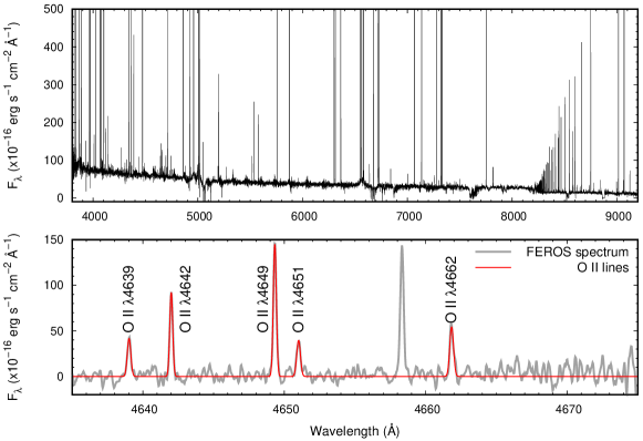
Figure 1: (upper panel) The FEROS spectrum of Hen3-1357 in the range between 3800 Å and 9200 Å. (lower panel) The FEROS spectrum in 4635-4675 Å (grey line) and the Gaussian fitting results for the O ii lines in this wavelength range (red line). The local continuum was subtracted out.

We secured the optical high-dispersion spectrum (3500-9200 Å) using the FEROS attached to the MPG ESO 2.2-m Telescope, La Silla, Chile (Prop.ID: 77.D-0478A, PI: M. Parthasarathy).

The weather condition was stable and clear throughout the night, and the seeing was 0.8-1.17″ (average: 0.97″) measured from the differential image motion monitor. FEROS’s fibers use 2.0″ apertures and provide simultaneously the object and sky spectra. The detector is the EEV CCD chip with 2048$\times$4096 pixels of 15$\times$15 µm square. We selected a 1$\times$1 on-chip binning and low gain mode. The atmospheric dispersion corrector (ADC) was not used during the observation. The exposure time was a single 2100 sec at airmass of 1.297-1.380. For the flux calibration and blaze function correction, we observed the standard star HR 3454 (Hamuy et al., 1992, 1994) at airmass $\sim$1.2. Since we did not use the ADC, a color-dependent displacement of the source from differential atmospheric refraction (DAR) might be present. However, we took Stingray nebula and HR 3454 at similar airmass. Therefore, we believe that DAR effect on the inferred extinction coefficients, the derived electron temperatures, and therefore on the derived ionic and elemental abundances would be largely reduced. We reduced the data with the echelle spectra reduction package Echelle in IRAF by a standard reduction manner including bias subtraction, removing scattered light, detector sensitivity correction, removing cosmic-ray hits, airmass extinction correction, flux density calibration, and all echelle order connection. Using the sky spectrum, we subtracted the sky-lines from the Hen3-1357 spectrum. The average resolving power ($\lambda$/$\Delta\lambda$) is 44 950, which was measured from the average full width at half maximum (FWHM) of over 300 Th-Ar comparison lines obtained for the wavelength calibrations. The signal-to-noise ratios per pixel were $\sim$2-12 for the continuum.

The resultant FEROS spectrum is presented in Fig. 1; the detected recombination lines (RLs) of O ii are shown in the lower panel. As far as we know, the N and O RLs such as N ii and O ii are detected in this PN for the first time.

2.3 Spitzer/IRS spectrum

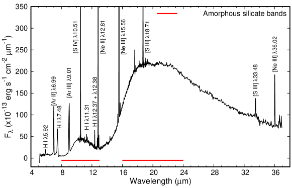
Figure 2: The Spitzer/IRS spectrum of Hen3-1357. The identified atomic lines and amorphous silicate features are denoted.

To investigate dust features and perform plasma diagnostics using fine-structure lines, we analyzed the mid-IR spectra taken by the Spitzer/Infrared Spectrograph (IRS; Houck et al., 2004) with the Short-Low (SL, 5.2-14.5 µm, the slit dimension: $\sim$3.6″ $\times$ 57″), Short-High (SH, 9.9-19.6 µm, 4.7″ $\times$ 11.3″), and Long-High modules (LH, 18.7-37.2 µm, 11.1″ $\times$ 22.3″).

We processed the BCD (program-ID: 3633, obs AORKEY: 11312640, PI: B. Matthew) using the data reduction packages SMART v.8.2.9 (Higdon et al., 2004) and IRSCLEAN v.2.1.1 provided by the SSC. We scaled the flux density of the reduced LH-spectrum to match with that of the reduced SH-spectrum in the overlapping wavelength, and we obtained the single 9.9-37.2 µm spectrum. Then, by the similar way, we combined this high-dispersion spectrum and the SL 5.2-14.5 µm spectrum into the single 5.2-37.2 µm spectrum.

We present the resultant spectrum in Fig. 2. The intensity peak positions of the identified atomic lines are marked by the vertical lines. We detected Ne, S, and Ar fine-structure lines. The spectrum clearly shows two broad features (indicated by the horizontal red lines) attributed to amorphous silicate grains; the features centered at 9 µm and 18 µm are due to the Si-O stretching mode and the O-Si-O bending mode, respectively. Perea-Calderón et al. (2009) reported that this PN is an O-rich dust object. We did not identify any carbon-based dust grains and molecules in the Spitzer/IRS spectrum. Thus, we can conclude that Hen3-1357 has an O-rich dust nebula.

3 Results

3.1 Scaling the flux density of the Spitzer/IRS spectrum

We performed a correction to recover the loss of light from Hen3-1357 by the slit.

First, using the AKARI/IRC 9.0 µm band photometry listed in Table 2, we scaled the flux density of the spectrum by considering the AKARI/IRC 9.0 µm filter transmission curve by a constant scaling factor of 0.951. Next, using this scaled spectrum and the Spitzer/IRAC 8.0 µm filter transmission curve, we measured the Spitzer/IRAC 8.0 µm band flux density. The measured value 1.90(–12) erg s^-1 cm^-2 µm^-1 is consistent with that the IRAC 8.0 µm photometry result.

AKARI/IRC 9.0 µm and Spitzer/IRAC 8.0 µm bands include atomic lines of H, Ne, S, and Ar certainly contributing to these two bands. As noted in §3.4, we did not find a significant difference between optical nebular line intensities relative to the H$\beta$ measured in 2006 and in 2011. This means that the ionization and elemental abundances of the nebula might not be changed in 2006-2011.

Our adopted scaling factor (0.951) indicates that the IR-band flux decreased by $\sim$5 % between 2005 and 2009. Therefore, we assume that mid-IR wavelength evolution had not dramatically changed in 2005-2009.

Taking into account these analyses, we scaled the flux density of the spectrum to match with the AKARI/IRC 9.0 µm band flux density.

3.2 The H$\beta$ flux of the entire nebula

The H$\beta$ flux of the entire nebula is necessary for setting the nebula’s hydrogen density structure in our SED modeling as well as for calculating the Ne^+,2+, S^2+,3+, and Ar^+,2+ to H⁺ number density ratios, and electron density $n_{\rm e}$ and temperature $T_{\rm e}$ using mid-IR fine-structure lines of these ions.

Since the H i 7.46 µm line is in the longer wavelength edge of the SL2 spectrum (5.13-7.60 µm) and also in the shorter edge of the SL1 spectrum (7.46-14.29 µm), we did not employ this line for estimating the H$\beta$ line flux of the entire nebula. Therefore, we obtained the H$\beta$ line flux by utilizing the theoretical H i $I$($n$ = 7-6 and 11-8)/$I$($n$ = 4-2) intensity ratio calculated by Storey & Hummer (1995), where $n$ is the principal quantum number. Note that a detected line at 12.37 µm (see Fig. 2) indeed composes of the H i $n$ = 7-6 at 12.37 µm and $n$ = 11-8 at 12.38 µm. From the $I$(12.37 µm + 12.38 µm)/$I$(H$\beta$) = 1.04(–2) in the case of an $n_{\rm e}$ = 10⁴ cm^-3 and a $T_{\rm e}$ = 10⁴ K (Storey & Hummer, 1995), we estimated the H$\beta$ flux of the entire nebula to be 9.83(–12) $\pm$ 7.33(–13) erg s^-1 cm^-2.

3.3 Flux measurements

Table 3: The derived $c$(H$\beta$) ratios. For the interstellar reddening correction to the FEROS spectrum, we adopted the average $c$(H$\beta$) = 8.27(–2) $\pm$ 3.47(–2)

$\lambda_{\rm lab.}$ (Å)	Line	$c$(H$\beta$)
3797.9	B10	8.25(–2) $\pm$ 6.43(–3)
3835.4	B9	3.25(–2) $\pm$ 5.17(–3)
3970.1	B7	7.39(–2) $\pm$ 2.95(–3)
4101.7	B6	4.38(–1) $\pm$ 3.56(–3)
4340.5	B5	1.34(–1) $\pm$ 5.16(–3)
8545.4	P15	2.03(–2) $\pm$ 1.04(–2)
8598.4	P14	3.84(–2) $\pm$ 2.54(–3)
8665.0	P13	7.49(–2) $\pm$ 2.48(–3)
8750.5	P12	6.64(–2) $\pm$ 1.98(–3)
9014.9	P10	1.18(–2) $\pm$ 2.25(–3)

We measured the fluxes of the emission lines by Gaussian fittings. Then, we corrected these fluxes using the following formula;

$$I(\lambda)=F(\lambda)~{}\cdot~{}10^{c({\rm H\beta})(1+f(\lambda))},$$ (1)

where $I$($\lambda$) is the de-reddened line flux, $F$($\lambda$) is the observed line flux, $f$($\lambda$) is the interstellar extinction function at $\lambda$ computed by the reddening law of Cardelli et al. (1989) with $R_{V}$ = 3.1, $c$(H$\beta$) is the reddening coefficient at H$\beta$.

We measured $c$(H$\beta$) values by comparing the observed ten Balmer and Paschen line ratios to H$\beta$ with the theoretical ratios of Storey & Hummer (1995) for a $T_{\rm e}$ = 10⁴ K and an $n_{\rm e}$ = 10⁴ cm^-3 under the Case B assumption. To reduce $c$(H$\beta$) estimation errors originated from the H i absorptions in the flux standard star HR 3454, we estimated $c$(H$\beta$) using different line ratios. The derived $c$(H$\beta$) values are listed in Table 3. Since the H$\alpha$ line was saturated, we did not calculate a $c$(H$\beta$) using the $F$(H$\alpha$)/$F$(H$\beta$) ratio. Finally, we adopted the average $c$(H$\beta$) = 8.27(–2) $\pm$ 3.47(–2). The scatter between the estimated $c$(H$\beta$) could be due to the H i absorptions’ depth of HR 3454 measured by Hamuy et al. (1992, 1994). We did not correct interstellar extinction for the Spitzer/IRS spectrum because the extinction is negligibly small in mid-IR wavelength.

For the year 2006, Reindl et al. (2014) reported $E(B-V)$ = 0.11, corresponding to $c$(H$\beta$) = 0.16. Although they did not give the uncertainty of $E(B-V)$, we assume $\delta\,E(B-V)$ = 0.02 from the fact that they measured $E(B-V)$ = 0.14 $\pm$ 0.02 in the year 1997. Thus, their $c$(H$\beta$) for the year 2006 is estimated to be 0.16 $\pm$ 0.03, which is consistent with ours.

In appendix Table Physical properties of the very young PN Hen3-1357 (Stingray Nebula) based on multiwavelength observations, we list 180 nebular lines detected in the FEROS spectrum. Since the [O iii] 5007 Å and H$\alpha$ lines were saturated, we do not list their fluxes. We calculated the average heliocentric radial velocity 12.30 km s^-1 and local standard of rest (LSR) radial velocity 12.29 km s^-1 using all the identified lines in the FEROS spectrum (1-$\sigma$ uncertainty is 0.25 km s^-1). Our heliocentric radial velocity is in good agreement with Arkhipova et al. (2013, 12.6 $\pm$ 1.7 km s^-1).

In appendix Table A2, we listed the fluxes of the identified 14 atomic gas emission-lines detected in the flux density scaled Spitzer/IRS spectrum, where the fluxes are normalized with respect to the H$\beta$ flux of the entire nebula.

3.4 Comparison of line fluxes between 2006 and 2011

We investigated the possibility of temporal variations of the emission line intensities by comparing our measurements with those of Arkhipova et al. (2013), who obtained the 3500-7200 Å low-resolution spectrum (FWHM = 4.5 Å) on 2011 June at the South African Astronomical Observatory (SAAO). In appendix Table A3. We list their measured line-intensities overlapped with ours. In 2006-2011, the nebular line fluxes did not significantly change. Indeed, the $I$($\lambda$)s in 2006 are very similar to those in 2011 ($I$(2011)/$I$(2006) = 1.11 $\pm$ 0.02, correlation factor is 0.995). Thus, the ionization and elemental abundances of the nebula might not be largely changed in 2006-2011. Variation in the $T_{\rm eff}$ of the central star by 5000 K to 10 000 K in 5 to 10 years interval might not immediately change the nebular morphology, parameters and abundances in the same time period.

3.5 Plasma-diagnostics

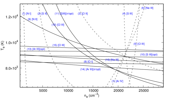
Figure 3: $n_{\rm e}$-$T_{\rm e}$ diagram based on CEL diagnostic line ratios. The dashed and thick lines with “(ID)“ indicate the $n_{\rm e}$ and $T_{\rm e}$-diagnostic curves generated by the line ratios listed in Table 4, respectively.

Table 4: Summary of plasma-diagnostics. As a comparison, the results by Arkhipova et al. (2013, for the year 2011) are listed in the last column.

$n_{\rm e}$-derivations (this work for the year 2006)					Arkhipova et al. (2013)
ID	Ion	Diagnostic line ratio	Ratio	Result (cm-3)	(cm-3)
(1)	[N i]	$I$(5197 Å)/$I$(5200 Å)	$1.59(0)~{}\pm~{}3.16(-2)$	$1390~{}\pm~{}90$	$~{}\cdots{}$
(2)	[S ii]	$I$(6716 Å)/$I$(6731 Å)	$3.23(-1)~{}\pm~{}7.30(-2)$	$5710~{}\pm~{}1790$	$8740~{}\pm~{}7701$
(3)	[O ii]	$I$(3726/29Å)/$I$(7320/30 Å)	$4.37(0)~{}\pm~{}1.17(-1)$	$17\,520~{}\pm~{}530$	$~{}\cdots{}$
(4)	[S iii]	$I$(18.7 µm)/$I$(33.5 µm)	$3.94(0)~{}\pm~{}3.32(-1)$	$21\,990~{}\pm~{}4840$	$~{}\cdots{}$
(5)	[Cl iii]	$I$(5517 Å)/$I$(5537 Å)	$4.86(-1)~{}\pm~{}1.69(-2)$	$23\,970~{}\pm~{}3120$	$~{}\cdots{}$
(6)	[Ne iii]	$I$(15.6 µm)/$I$(36.0 µm)	$1.56(+1)~{}\pm~{}9.67(-1)$	$22\,750~{}\pm~{}5850$	$~{}\cdots{}$
(7)	[Ar iv]	$I$(4711 Å)/$I$(4740 Å)	$4.88(-1)~{}\pm~{}4.55(-2)$	$22\,720~{}\pm~{}4360$	$~{}\cdots{}$
	H i	Paschen decrement		10 000 – 20 000	$~{}\cdots{}$
$T_{\rm e}$-derivations (this work for the year 2006)					Arkhipova et al. (2013)
ID	Ion	Diagnostic line ratio	Ratio	Result (K)	(K)
(8)	[O i]	$I$(6300/63 Å)/$I$(5577 Å)	$9.69(+1)~{}\pm~{}2.57(0)$	$8470~{}\pm~{}70$	$~{}\cdots{}$
(9)	[N ii]	$I$(6548/83 Å)/$I$(5755 Å)	$6.38(+1)~{}\pm~{}1.55(0)$	$9280~{}\pm~{}100$	$11\,066~{}\pm~{}1752$
(10)	[S iii]	$I$(9069 Å)/$I$(6312 Å)	$1.22(+1)~{}\pm~{}6.34(-1)$	$8880~{}\pm~{}180$	$11\,831~{}\pm~{}2286$
(11)	[S iii]	$I$(18.7/33.5 µm)/$I$(9069 Å)	$1.38(0)~{}\pm~{}7.82(-2)$	$7430~{}\pm~{}280$	$~{}\cdots{}$
(12)	[Cl iii]	$I$(5517/37 Å)/$I$(8434/8501 Å)	$2.03(+1)~{}\pm~{}4.54(0)$	$7490~{}\pm~{}850$	$~{}\cdots{}$
(13)	[Ar iii]	$I$(7135/7751 Å)/$I$(5191 Å)	$2.09(+2)~{}\pm~{}1.14(+1)$	$8670~{}\pm~{}150$	$~{}\cdots{}$
(14)	[Ar iii]	$I$(9.01 µm)/$I$(7135/7751 Å)	$9.70(-1)~{}\pm~{}4.27(-2)$	$8400~{}\pm~{}310$	$~{}\cdots{}$
(15)	[O iii]	$I$(4959 Å)/$I$(4363 Å)	$5.91(+1)~{}\pm~{}7.27(-1)$	$9420~{}\pm~{}40$	$11\,553~{}\pm~{}1579$
(16)	[Ne iii]	$I$(15.6 µm)/$I$(3869/3968 Å)	$1.92(0)~{}\pm~{}7.34(-2)$	$8560~{}\pm~{}70$	$~{}\cdots{}$
$T_{\rm e}$(PJ)		($I_{\lambda}$(8194 Å)-$I_{\lambda}$(8169 Å))/$I$(P11)	$2.16(-2)~{}\pm~{}2.53(-3)$	$8090~{}\pm~{}1680$	$~{}\cdots{}$
$T_{\rm e}$(He i)	He i	$I$(7281 Å)/$I$(6678 Å)	$1.83(-1)~{}\pm~{}7.38(-3)$	$8340~{}\pm~{}330$	$~{}\cdots{}$
$T_{\rm e}$(He i)	He i	$I$(7281 Å)/$I$(5876 Å)	$4.95(-2)~{}\pm~{}1.80(-3)$	$7980~{}\pm~{}360$	$~{}\cdots{}$

In forbidden line analysis, we employed the NEBULAR package by Shaw & Dufour (1995). In recombination line analysis, we used private softwares. In both of emission line analyses, we adopted effective recombination coefficients, transition probabilities, and effective collision strengths listed in Otsuka et al. (2010, their Table 7).

We performed plasma diagnostics using collisionally excited lines (CELs) and RLs. We greatly increase the results, comparing to Parthasarathy et al. (1993) who obtained one $n_{\rm e}$ and two $T_{\rm e}$ using the optical spectrum taken in 1992 and Arkhipova et al. (2013) who deduced one $n_{\rm e}$ and four $T_{\rm e}$ based on the 3500-7200 Å spectrum taken in 2011. In Table 4, we list the diagnostic line ratios to derive $n_{\rm e}$ and $T_{\rm e}$ and the resultant values. In Fig. 3, we present the $n_{\rm e}$-$T_{\rm e}$ diagram using the diagnostic CEL ratios. “opt” indicates the result by the optical forbidden line ratio; e.g., [S iii] $I$(9069 Å)/$I$(6312 Å) ratio. “ir/opt” means the result using the mid-IR fine-structure lines and optical forbidden line; e.g., [S iii] $I$(18.7/33.5 µm)/$I$(9067 Å) ratio. We bear in mind that CEL emissivities are in general sensitive to $n_{\rm e}$ and $T_{\rm e}$, accordingly CEL ionic abundances depend on a selection of $n_{\rm e}$ and $T_{\rm e}$.

First, we calculated $n_{\rm e}$ using CELs. The $n_{\rm e}$-$T_{\rm e}$ diagram indicates that the average $n_{\rm e}$ is in a range from $\sim$2000 cm^-3 in neutral gas regions (by the $n_{\rm e}$([N i]) curve, ID(1)) and $\sim$20 000 cm^-3 in highly ionized gas regions (by the $n_{\rm e}$([Ar iv]) curve, ID(7)) and the average $T_{\rm e}$ is $\sim$8000-10 000 K. We derived all $n_{\rm e}$ by adopting a constant $T_{\rm e}$ = 9 000 K.

Next, we calculated $T_{\rm e}$([O i]) by adopting $n_{\rm e}$([N i]), $T_{\rm e}$([Ar iii]) by the average $n_{\rm e}$ = 22 980 cm^-3 between $n_{\rm e}$([S iii]) and $n_{\rm e}$([Cl iii]), $T_{\rm e}$([S iii]) by $n_{\rm e}$([S iii]), $T_{\rm e}$([Cl iii]) by $n_{\rm e}$([Cl iii]), and both $T_{\rm e}$([O iii]) and $T_{\rm e}$([Ne iii]) by adopting $n_{\rm e}$([Ne iii]), respectively.

To obtain $T_{\rm e}$([O ii]), $n_{\rm e}$([O ii], and $T_{\rm e}$([N ii]) which are representative $n_{\rm e}$ and $T_{\rm e}$ in lower ionization regions, we subtracted respective contributions from O²⁺ and N²⁺ recombination to the [O ii] 7320/30 Å lines and the [N ii] 5755 Å line. We calculated the contributions to these lines, $I_{\rm R}$([O ii] 7320/30 Å) and $I_{\rm R}$([N ii] 5755 Å) by using the following equations by Liu et al. (2000).

$$\frac{I_{\rm R}({\rm[O\,{\sc II}]\,7320/30\,{\AA}})}{I({\rm H\beta})}=9.36\left(\frac{T_{\rm e}}{10^{4}}\right)^{0.44}\frac{n({\rm O^{2+}})}{n({\rm H^{+}})},$$ (2)

$$\frac{I_{\rm R}({\rm[N\,{\sc II}]\,5755\,{\AA}})}{I({\rm H\beta})}=3.19\left(\frac{T_{\rm e}}{10^{4}}\right)^{0.33}\frac{n({\rm N^{2+}})}{n({\rm H^{+}})}.$$ (3)

Here $n$(O²⁺)/$n$(H⁺) and $n$(N²⁺)/$n$(H⁺) are the number density ratios of the O² and N⁺ with respect to the H⁺, respectively.

We adopted the CEL O²⁺ = 1.87(–4) $\pm$ 1.39(–6) (see §3.6) in order to obtain the $I_{\rm R}$([O ii] 7320/30 Å) = 0.16 $\pm$ 0.01, where $I$(H$\beta$) = 100. Based on the result that the CEL O²⁺ is consistent with the RL O²⁺, we assumed that the CEL N²⁺ could be very close to the RL N²⁺. Here, we adopted the RL N²⁺ = 6.97(–5) $\pm$ 3.17(–5) (see §3.6) to calculate the $I_{\rm R}$([N ii] 5755 Å) of 0.33 $\pm$ 0.05.

The [O ii] $I$(3726 Å)/$I$(3729 Å) ratio is a $n_{\rm e}$ indicator and $I$(3726/29 Å)/$I$(7320/30 Å) ratio is sensitive to both $T_{\rm e}$ and $n_{\rm e}$. In Hen3-1357, $n_{\rm e}$ exceeds the critical density of the [O ii] 3726/29 Å lines, so that the $I$(3726 Å)/$I$(3729 Å) ratio could not give reliable $n_{\rm e}$. Therefore, we used the $I$(3726/29 Å)/$I$(7320/30 Å) ratio to derive an $n_{\rm e}$ required for the N⁺, O⁺, Cl⁺, Ar⁺, and Fe²⁺ calculations. We obtained $n_{\rm e}$([O ii]) by adopting a constant $T_{\rm e}$ = 9000 K, and then $T_{\rm e}$([N ii]) using this $n_{\rm e}$([O ii]) = 17 520 cm^-3.

We found the discrepancy between two $T_{\rm e}$([S iii]) values (IDs 10 and 11). This might be due to the underestimated [S iii] 9069 Å, which is appeared in the red wavelength edge of the FEROS spectrum. Because the ionic S²⁺ abundance from this line is $\sim$14 $\%$ smaller than that from the fine-structure [S iii] lines, which is insensitive to $T_{\rm e}$ (see Table 5). As we explained in §,2.2, the differential atmospheric refraction (DAR) effect might have affected [S iii] 9069 Å, although we cannot exactly estimate how much light of [S iii] 9069 Å line we lost. DAR effect might affect widely separated diagnostic line intensity ratios. However, for the S²⁺ abundance estimate, we adopted the average $T_{\rm e}$ between two $T_{\rm e}$([S iii]). Thus, we reduced the effects by inconsistency between these two $T_{\rm e}$([S iii]).

Similarly, if we underestimate the [O ii] 7320/30 Å intensity by $\sim$14%, which is an expected value from the above analysis for the S²⁺ abundance, we obtain $n_{\rm e}$([O ii]) = 20 300 cm^-3. Then using this $n_{\rm e}$([O ii]), we obtain $T_{\rm e}$([N ii]) = 9010 K. Under these $n_{\rm e}$([O ii]) and $T_{\rm e}$([N ii]), the N⁺, O⁺, Cl⁺, and Fe²⁺ abundances would increase by $\sim$12 %. Even if DAR effect is present in our FEROS spectrum, the potential error of $c$(H$\beta$), $T_{\rm e}$ and $n_{\rm e}$, and ionic/elemental abundances caused by DAR effect would be $\sim$15 % or less. Hence, our conclusion on these physical parameters derived from the CELs and the RLs does not change.

Finally, we calculated $T_{\rm e}$ and $n_{\rm e}$ using He i lines and H i Paschen series. We calculated $T_{\rm e}$(He i) using He i $I$(7281 Å)/$I$(6678 Å) and $I$(7281 Å)/$I$(5876 Å) ratios using the recombination coefficients in a constant $n_{\rm e}$ = 10⁴ cm^-3 provided by Benjamin et al. (1999). We calculated the Paschen jump $T_{\rm e}$(PJ) by using equation (7) of Fang & Liu (2011). The H i P11 line is in an echelle order gap. Therefore, we obtained the expected $I$(P11) using the observed H i P12 line and the theoretical $I$(P11)/$I$(P12) ratio of 1.30 in $n_{\rm e}$ $\sim$10²-10⁵ cm^-3 and $T_{\rm e}$ $\sim$5000-15 000 K (Storey & Hummer, 1995). Thus, we obtained $n_{\rm e}$ $\sim$10 000-20 000 cm^-3 by comparing the observed $I$(P$n$)/$I$(P10) ratios ($n$ is from 12 to 42) and the theoretical calculations under the Case B assumption and $T_{\rm e}$(PJ) = 8090 K by Storey & Hummer (1995).

As a comparison, the results by Arkhipova et al. (2013, for the year 2011) are listed in the last column. Arkhipova et al. (2013) reported $T_{\rm e}$([O iii]) = 11 553 $\pm$ 1579 K, $T_{\rm e}$([O ii]) = 11 983 $\pm$ 770 K, $T_{\rm e}$([N ii]) = 11 066 $\pm$ 1752 K, $T_{\rm e}$([S iii]) = 11 831 $\pm$ 2286 K, and $n_{\rm e}$([S ii]) = 8740 $\pm$ 7701 cm^-3, respectively. The difference between their $T_{\rm e}$([O iii]) and ours is due to the [O iii] 4363 Å intensity (see appendix Table A3). Under a constant $n_{\rm e}$, the $T_{\rm e}$([O iii]) becomes higher as the [O iii] $I$(4959/5007 Å)/$I$(4363 Å) ratio becomes lower. The [N ii] $n_{\rm e}$-$T_{\rm e}$ curve in Fig. 3 suggests that the discrepancy in $T_{\rm e}$([N ii]) could be due to the difference in adopted $n_{\rm e}$.

3.6 Ionic abundance derivations

Table 5: The ionic abundances derived using CELs.

Elem.	Ion	$\lambda_{\rm lab.}$	$I$($\lambda$)	$n$(Xm+)/$n$(H+)	Elem.	Ion	$\lambda_{\rm lab.}$	$I$($\lambda$)	$n$(Xm+)/$n$(H+)
(X)	(Xm+)		($I$(H$\beta$) = 100)		(X)	(Xm+)		($I$(H$\beta$) = 100)
(1)	(2)	(3)	(4)	(5)	(6)	(7)	(8)	(9)	(10)
N(CEL)	N0	5197.90 Å	$3.63(-1)~{}\pm~{}4.38(-3)$	$1.11(-6)~{}\pm~{}3.46(-8)$	S	S+	4068.60 Å	$4.47(0)~{}\pm~{}8.61(-2)$	$1.13(-6)~{}\pm~{}1.37(-7)$
		5200.26 Å	$2.28(-1)~{}\pm~{}3.59(-3)$	$1.07(-6)~{}\pm~{}1.82(-8)$			4076.35 Å	$1.51(0)~{}\pm~{}2.90(-2)$	$1.17(-6)~{}\pm~{}1.43(-7)$
			Average	${\bf 1.09(-6)}~{}\pm~{}{\bf 2.83(-8)}$			6716.44 Å	$6.07(0)~{}\pm~{}1.54(-1)$	$9.55(-7)~{}\pm~{}1.57(-7)$
	N+	5754.64 Å	$2.55(0)~{}\pm~{}3.87(-2)$	$3.61(-5)~{}\pm~{}2.41(-6)$			6730.81 Å	$1.25(+1)~{}\pm~{}3.19(-1)$	$1.07(-6)~{}\pm~{}1.13(-7)$
		6548.04 Å	$4.10(+1)~{}\pm~{}9.67(-1)$	$3.60(-5)~{}\pm~{}1.24(-6)$				Average	${\bf 1.06(-6)}~{}\pm~{}{\bf 1.30(-7)}$
		6583.46 Å	$1.21(+2)~{}\pm~{}2.91(0)$	$3.60(-5)~{}\pm~{}1.25(-6)$		S2+	6312.10 Å	$~{}1.03(0)~{}\pm~{}2.19(-2)$	$6.19(-6)~{}\pm~{}9.21(-7)$
			Average	${\bf 3.60(-5)}~{}\pm~{}{\bf 1.27(-6)}$			9068.60 Å	$1.26(+1)~{}\pm~{}5.96(-1)$	$4.90(-6)~{}\pm~{}3.88(-7)$
			ICF(N(CEL))	$3.09~{}\pm~{}0.17$			18.71 µm	$1.39(+1)~{}\pm~{}4.65(-1)$	$5.60(-6)~{}\pm~{}8.07(-7)$
				${\bf 1.11(-4)}~{}\pm~{}{\bf 7.39(-6)}$			33.48 µm	$3.52(0)~{}\pm~{}2.72(-1)$	$5.63(-6)~{}\pm~{}1.31(-6)$
O(CEL)	O0	5577.34 Å	$2.19(-1)~{}\pm~{}4.49(-3)$	$6.06(-5)~{}\pm~{}3.96(-6)$				Average	${\bf 5.34(-6)}~{}\pm~{}{\bf 6.98(-7)}$
		6300.30 Å	$1.61(+1)~{}\pm~{}3.39(-1)$	$6.06(-5)~{}\pm~{}2.48(-6)$		S3+	10.51 µm	$7.76(0)~{}\pm~{}2.66(-1)$	$4.18(-7)~{}\pm~{}6.52(-8)$
		6363.78 Å	$5.10(0)~{}\pm~{}1.11(-1)$	$6.00(-5)~{}\pm~{}2.46(-6)$				ICF(S)	1.00
			Average	${\bf 6.05(-5)}~{}\pm~{}{\bf 2.49(-6)}$					${\bf 6.82(-6)}~{}\pm~{}{\bf 7.13(-7)}$
	O+	3726.03 Å	$1.01(+2)~{}\pm~{}2.62(0)$	$2.67(-4)~{}\pm~{}1.08(-5)$	Ar	Ar+	6.99 µm	$7.43(0)~{}\pm~{}2.53(-1)$	$7.15(-7)~{}\pm~{}2.48(-8)$
		3728.81 Å	$3.76(+1)~{}\pm~{}9.79(-1)$	$2.56(-4)~{}\pm~{}9.88(-6)$		Ar2+	5191.82 Å	$6.41(-2)~{}\pm~{}3.11(-3)$	$1.94(-6)~{}\pm~{}3.27(-7)$
		7320/7330 Å	$3.18(+1)~{}\pm~{}5.56(-1)$	$2.98(-4)~{}\pm~{}2.32(-5)$			7135.80 Å	$1.08(+1)~{}\pm~{}3.22(-1)$	$1.47(-6)~{}\pm~{}1.16(-7)$
			Average	${\bf 2.70(-4)}~{}\pm~{}{\bf 1.29(-5)}$			7751.10 Å	$2.63(0)~{}\pm~{}9.57(-2)$	$1.50(-6)~{}\pm~{}1.23(-7)$
	O2+	4363.21 Å	$2.46(0)~{}\pm~{}2.96(-2)$	$1.88(-4)~{}\pm~{}9.02(-6)$			9.01 µm	$1.30(+1)~{}\pm~{}4.71(-1)$	$1.70(-6)~{}\pm~{}6.56(-8)$
		4931.23 Å	$~{}5.46(-2)~{}\pm~{}2.92(-3)$	$1.80(-4)~{}\pm~{}9.67(-6)$				Average	${\bf 1.59(-6)}~{}\pm~{}{\bf 9.25(-8)}$
		4958.91 Å	$1.46(+2)~{}\pm~{}3.80(-1)$	$1.87(-4)~{}\pm~{}1.26(-6)$		Ar3+	4711.37 Å	$3.39(-2)~{}\pm~{}3.05(-3)$	$2.12(-8)~{}\pm~{}2.29(-9)$
			Average	${\bf 1.87(-4)}~{}\pm~{}{\bf 1.39(-6)}$			4740.16 Å	$6.95(-2)~{}\pm~{}1.72(-3)$	$2.09(-8)~{}\pm~{}8.27(-10)$
			ICF(O(CEL))	1.00				Average	${\bf 2.10(-8)}~{}\pm~{}{\bf 1.31(-9)}$
				${\bf 4.57(-4)}~{}\pm~{}{\bf 1.30(-5)}$				ICF(Ar)	1.00
Ne	Ne+	12.81 µm	$4.67(+1)~{}\pm~{}1.55(0)$	$7.23(-5)~{}\pm~{}2.45(-6)$					${\bf 2.32(-6)}~{}\pm~{}{\bf 9.57(-8)}$
	Ne2+	3869.06 Å	$4.03(+1)~{}\pm~{}9.46(-1)$	$8.77(-5)~{}\pm~{}4.07(-6)$	Fe	Fe2+	4658.05 Å	$1.11(-1)~{}\pm~{}2.50(-3)$	$6.71(-8)~{}\pm~{}2.80(-9)$
		3967.79 Å	$1.00(+1)~{}\pm~{}2.16(-1)$	$7.22(-5)~{}\pm~{}3.29(-6)$			4701.53 Å	$4.65(-2)~{}\pm~{}3.17(-3)$	$7.17(-8)~{}\pm~{}5.65(-9)$
		15.56 µm	$9.67(+1)~{}\pm~{}3.19(0)$	$8.38(-5)~{}\pm~{}4.54(-6)$			4733.91 Å	$2.58(-2)~{}\pm~{}2.74(-3)$	$8.82(-8)~{}\pm~{}1.01(-8)$
		36.02 µm	$6.18(0)~{}\pm~{}3.23(-1)$	$8.57(-5)~{}\pm~{}1.01(-5)$			4754.69 Å	$2.86(-2)~{}\pm~{}3.64(-3)$	$9.18(-8)~{}\pm~{}1.21(-8)$
			Average	${\bf 8.41(-5)}~{}\pm~{}{\bf 4.56(-6)}$			5270.40 Å	$5.89(-2)~{}\pm~{}2.40(-3)$	$6.76(-8)~{}\pm~{}3.48(-9)$
			ICF(Ne)	1.00				Average	${\bf 7.26(-8)}~{}\pm~{}{\bf 5.11(-9)}$
				${\bf 1.56(-4)}~{}\pm~{}{\bf 4.77(-6)}$				ICF(Fe)	$2.30~{}\pm~{}0.14$
Cl	Cl+	8578.69 Å	$3.04(-1)~{}\pm~{}1.35(-2)$	$1.64(-8)~{}\pm~{}8.17(-10)$					${\bf 1.67(-7)}~{}\pm~{}{\bf 1.57(-8)}$
		9123.60 Å	$1.03(-1)~{}\pm~{}5.46(-3)$	$2.12(-8)~{}\pm~{}1.23(-9)$
			Average	${\bf 1.76(-8)}~{}\pm~{}{\bf 9.22(-10)}$
	Cl2+	5517.72 Å	$1.17(-1)~{}\pm~{}3.39(-3)$	$1.02(-7)~{}\pm~{}3.71(-8)$
		5537.89 Å	$2.40(-1)~{}\pm~{}4.59(-3)$	$1.02(-7)~{}\pm~{}3.93(-8)$
		8434.00 Å	$7.76(-3)~{}\pm~{}1.23(-3)$	$1.18(-7)~{}\pm~{}7.51(-8)$
		8500.20 Å	$9.76(-3)~{}\pm~{}3.70(-3)$	$1.18(-7)~{}\pm~{}8.55(-8)$
			Average	${\bf 1.03(-7)}~{}\pm~{}{\bf 4.06(-8)}$
			ICF(Cl)	$1.01~{}\pm~{}0.06$
				${\bf 1.21(-7)}~{}\pm~{}{\bf 4.16(-8)}$

Table 6: The ionic abundances derived using RLs.

Elem.	Ion	$\lambda_{\rm lab.}$	$I$($\lambda$)	$n$(Xm+)/$n$(H+)
(X)	(Xm+)	(Å)	($I$(H$\beta$) = 100)
He	He+	4120.81	$1.77(-1)~{}\pm~{}4.80(-3)$	$9.95(-2)~{}\pm~{}5.32(-3)$
		4387.93	$4.39(-1)~{}\pm~{}6.42(-3)$	$7.18(-2)~{}\pm~{}4.73(-3)$
		4437.55	$6.64(-2)~{}\pm~{}4.31(-3)$	$8.53(-2)~{}\pm~{}6.61(-3)$
		4471.47	$4.63(0)~{}\pm~{}4.85(-2)$	$9.34(-2)~{}\pm~{}5.22(-3)$
		4713.22	$6.68(-1)~{}\pm~{}6.70(-3)$	$1.14(-1)~{}\pm~{}9.20(-3)$
		4921.93	$1.21(0)~{}\pm~{}4.45(-3)$	$9.05(-2)~{}\pm~{}4.65(-3)$
		5015.68	$2.16(0)~{}\pm~{}1.19(-2)$	$7.69(-2)~{}\pm~{}3.63(-3)$
		5047.74	$1.68(-1)~{}\pm~{}3.09(-3)$	$8.24(-2)~{}\pm~{}4.52(-3)$
		5875.60	$1.47(+1)~{}\pm~{}2.62(-1)$	$1.02(-1)~{}\pm~{}6.54(-3)$
		6678.15	$3.97(0)~{}\pm~{}9.94(-2)$	$9.79(-2)~{}\pm~{}5.74(-3)$
		7281.35	$7.26(-1)~{}\pm~{}2.30(-2)$	$8.37(-2)~{}\pm~{}4.43(-3)$
			Average	${\bf 9.69(-2)}~{}\pm~{}{\bf 5.88(-3)}$
			ICF(He)	$1.00$
				${\bf 9.69(-2)}~{}\pm~{}{\bf 5.88(-3)}$
C(RL)	C2+	4267.18	$1.03(-1)~{}\pm~{}4.54(-3)$	$9.66(-5)~{}\pm~{}3.06(-5)$
		6578.05	$5.05(-2)~{}\pm~{}3.71(-3)$	$9.84(-5)~{}\pm~{}3.88(-5)$
			Average	${\bf 9.72(-5)}~{}\pm~{}{\bf 3.33(-5)}$
			ICF(C(RL))	$1.48~{}\pm~{}0.22$
				${\bf 1.44(-4)}~{}\pm~{}{\bf 5.38(-5)}$
N(RL)	N2+	4630.54	$2.02(-2)~{}\pm~{}2.59(-3)$	$9.27(-5)~{}\pm~{}4.21(-5)$
		5679.56	$1.69(-2)~{}\pm~{}2.30(-3)$	$4.23(-5)~{}\pm~{}1.93(-5)$
			Average	${\bf 6.97(-5)}~{}\pm~{}{\bf 3.17(-5)}$
			ICF(N(RL))	$1.48~{}\pm~{}0.22$
				${\bf 1.03(-4)}~{}\pm~{}{\bf 4.94(-5)}$
O(RL)	O2+	4069.62	$2.65(-2)~{}\pm~{}3.24(-3)$	$2.78(-4)~{}\pm~{}7.04(-5)$
		4069.88	$3.84(-2)~{}\pm~{}4.55(-3)$	$2.52(-4)~{}\pm~{}6.61(-5)$
		4072.15	$5.68(-2)~{}\pm~{}2.51(-3)$	$2.34(-4)~{}\pm~{}5.45(-5)$
		4075.86	$7.55(-2)~{}\pm~{}5.04(-3)$	$2.26(-4)~{}\pm~{}5.34(-5)$
		4104.99	$4.05(-2)~{}\pm~{}4.28(-3)$	$3.64(-4)~{}\pm~{}9.07(-5)$
		4153.30	$3.10(-2)~{}\pm~{}1.60(-3)$	$4.04(-4)~{}\pm~{}9.69(-5)$
		4349.43	$3.34(-2)~{}\pm~{}2.39(-3)$	$1.70(-4)~{}\pm~{}3.92(-5)$
		4366.90	$3.41(-2)~{}\pm~{}2.60(-3)$	$4.48(-4)~{}\pm~{}1.07(-4)$
		4638.86	$3.44(-2)~{}\pm~{}3.53(-3)$	$3.06(-4)~{}\pm~{}7.73(-5)$
		4641.81	$6.37(-2)~{}\pm~{}2.21(-3)$	$2.38(-4)~{}\pm~{}5.35(-5)$
		4649.13	$1.03(-1)~{}\pm~{}2.72(-3)$	$2.13(-4)~{}\pm~{}4.79(-5)$
		4650.84	$3.42(-2)~{}\pm~{}1.93(-3)$	$3.28(-4)~{}\pm~{}7.57(-5)$
		4661.63	$4.79(-2)~{}\pm~{}2.17(-3)$	$3.83(-4)~{}\pm~{}8.68(-5)$
		4676.23	$3.19(-2)~{}\pm~{}5.12(-3)$	$3.34(-4)~{}\pm~{}9.09(-5)$
			Average	${\bf 2.82(-4)}~{}\pm~{}{\bf 6.73(-5)}$
			ICF(O(RL))	$2.45~{}\pm~{}0.07$
				${\bf 6.89(-4)}~{}\pm~{}{\bf 1.66(-4)}$

Table 7: Comparison of the ionic abundances in 2006 by us and 2011 by Arkhipova et al. (2013).

Ion (Xm+)	$n$(Xm+)/$n$(H+) in 2006	$n$(Xm+)/$n$(H+) in 2011
He+	9.69(–2) $\pm$ 5.88(–3)	9.70(–2) $\pm$ 8.00(–3)
N+	3.60(–5) $\pm$ 1.27(–6)	5.81(–5) $\pm$ 2.31(–5)
O+	2.70(–4) $\pm$ 1.29(–5)	9.10(–5) $\pm$ 7.16(–5)
O2+(CEL)	1.87(–4) $\pm$ 1.39(–6)	1.01(–4) $\pm$ 4.26(–5)
Ne2+	8.41(–5) $\pm$ 4.56(–6)	3.46(–5) $\pm$ 1.76(–5)
S+	1.06(–6) $\pm$ 1.30(–7)	9.34(–7) $\pm$ 5.70(–7)
S2+	5.34(–6) $\pm$ 6.98(–7)	1.43(–6) $\pm$ 1.13(–6)
Ar2+	1.59(–6) $\pm$ 9.25(–8)	1.00(–6) $\pm$ 4.26(–7)

In appendix Table A4, we list $n_{\rm e}$ and $T_{\rm e}$ adopted for calculating each ionic abundance. We determined these values by referring to the $n_{\rm e}$-$T_{\rm e}$ diagram and taking the ionization potential (IP) of the targeting ion into account. We calculated the CEL ionic abundances by solving an equation of population at multiple energy levels (from two energy levels for Ne⁺ and Ar⁺ and 33 levels for Fe²⁺) under the listed $n_{\rm e}$ and $T_{\rm e}$. We adopted a constant $n_{\rm e}$ = 10⁴ cm^-3 and the average $T_{\rm e}$(He i) 8160 K to calculate the He⁺. For the RL C²⁺, N²⁺, and O²⁺, we adopted $n_{\rm e}$ = 10⁴ cm^-3 and $T_{\rm e}$(PJ).

We summarize the resultant CEL and RL ionic abundances in Tables 5 and 6, respectively. When we detected two or more lines of a target ion, we derived each ionic abundance using each line intensity. Then, we adopted the weight-average value as the representative ionic abundance as listed in the last line of each ion by boldface. We give the 1-$\sigma$ uncertainty of each ionic abundance, which accounts for the uncertainties of line fluxes (including $c$(H$\beta$) uncertainty), $T_{\rm e}$, and $n_{\rm e}$.

The CEL abundances calculated using the optical lines are well consistent with ones using mid-IR fine-structure lines, indicating that the calculated CEL ionic abundances are the results based on proper selections of $T_{\rm e}$ in particular and accurate scaling flux of the Spitzer/IRS spectrum.

We obtained the RL N²⁺ and O²⁺ in this PN for the first time. The higher multiplet lines are in general insensitive to Case A or Case B assumptions and reliable because these lines are less affected by both resonance fluorescence by starlight and recombination from higher terms. The consistency between the RL C²⁺ abundance by the multiple V6 4267.18 Å line and by the V2 6578.05 Å line indicates that the RL C²⁺ from both lines can be reliable. We can have the similar conclusion for the RL O²⁺ and N²⁺ abundances. The RL O²⁺ abundances are well consistent among the O ii V1 4638/42/49/51/62/76 Å, V2 4349/67 Å, V10 4069.6/69.9/72/76 Å, V19 4153 Å, and V20 4105 Å lines. The RL N²⁺ abundances are derived using the V3 5679 Å and 4631 Å lines.

As compared in Table 7, our ionic abundances agree with Arkhipova et al. (2013). However, we found the obvious discrepancies in the Ne²⁺ and S²⁺. Their S²⁺ seems to be derived using the auroral line [S iii] 6312 Å. Although they did not report the detection of any [Ne iii] lines in their spectrum taken in 2011, we assume that they derived the Ne²⁺ using nebular [Ne iii] lines. The Ne²⁺ and S²⁺ differences between Arkhipova et al. (2013) and us are due to the adopted $T_{\rm e}$. We stress that our adopted $T_{\rm e}$ for the Ne²⁺ and S²⁺ is determined using the [Ne iii] and [S iii] fine-structure, nebular, and auroral lines. For instance, if we adopt their $T_{\rm e}$([O iii]) = 11 553 K to calculate the Ne²⁺ using the nebular [Ne iii] lines, the volume emissivities of these [Ne iii] lines become 2.66 times higher than those in our adopted $T_{\rm e}$ = 8560 K. Accordingly, the Ne²⁺ is down to 3.18(–5), which is consistent with Arkhipova et al. (2013). However, since the emissivities of the fine-structure [Ne iii] lines do not largely change even in both 8560 K by ours and 11 553 K by Arkhipova et al. (2013), the Ne²⁺ abundances using the fine-structure [Ne iii] lines keep 8.38(–5) (from the [Ne iii] 15.56 µm line) and 8.57(–5) (from the [Ne iii] 36.02 µm line). That is, we find out the spurious Ne²⁺ derivation discrepancy between the nebular and the fine-structure lines. We confirmed that the similar conclusion can apply for the S²⁺. Thus, if the nebula condition is in a steady state and had not dramatically changed in 2006-2011, we can conclude that our Ne²⁺ and S²⁺ are more reliable.

3.7 Elemental abundance derivations using the ICFs

Table 8: Elemental abundances. The C(CEL) is an expected value estimated by adopting the RL C/O ratio.

Elem. (X)	$n$(X)/$n$(H)	$\epsilon$(X)	[X/H]
He	$9.69(-2)~{}\pm~{}5.88(-3)$	$10.99~{}\pm~{}0.03$	$+0.06~{}\pm~{}0.03$
C(RL)	$1.44(-4)~{}\pm~{}5.38(-5)$	$8.16~{}\pm~{}0.16$	$-0.23~{}\pm~{}0.17$
C(CEL)	$9.54(-5)~{}\pm~{}4.26(-5)$	$7.98~{}\pm~{}0.19$	$-0.40~{}\pm~{}0.20$
N(RL)	$1.03(-4)~{}\pm~{}7.39(-6)$	$8.01~{}\pm~{}0.03$	$+0.15~{}\pm~{}0.12$
N(CEL)	$1.11(-4)~{}\pm~{}7.39(-6)$	$8.05~{}\pm~{}0.03$	$+0.19~{}\pm~{}0.12$
O(RL)	$6.89(-4)~{}\pm~{}1.66(-4)$	$8.84~{}\pm~{}0.10$	$+0.11~{}\pm~{}0.13$
O(CEL)	$4.57(-4)~{}\pm~{}1.30(-5)$	$8.66~{}\pm~{}0.01$	$-0.07~{}\pm~{}0.07$
Ne	$1.56(-4)~{}\pm~{}4.77(-6)$	$8.19~{}\pm~{}0.01$	$+0.14~{}\pm~{}0.10$
S	$6.82(-6)~{}\pm~{}7.13(-7)$	$6.83~{}\pm~{}0.05$	$-0.33~{}\pm~{}0.05$
Cl	$1.21(-7)~{}\pm~{}4.16(-8)$	$5.08~{}\pm~{}0.15$	$-0.17~{}\pm~{}0.16$
Ar	$2.32(-6)~{}\pm~{}9.57(-8)$	$6.37~{}\pm~{}0.02$	$-0.13~{}\pm~{}0.10$
Fe	$1.67(-7)~{}\pm~{}1.57(-8)$	$5.22~{}\pm~{}0.04$	$-2.24~{}\pm~{}0.09$

By introducing the ionization correction factor (ICF), we inferred the nebular abundances from their ionic abundances. We calculated these ICF(X)s derived based on the fraction of the observed ionic abundances with similar ionization potentials to the target element. The ICF(X) of element X is listed in the last line of each element of Tables 5 and 6. The abundance of the element X $n$(X)/$n$(H) corresponds to the value derived from the ICF(X) $\cdot$ $\Sigma_{\rm m=1}$$n$(X^m+)/$n$(H⁺). We will compare these ICFs(X) based on IPs with those calculated by Cloudy photoionization model later.

As shown in §3.6, we obtained the O(CEL), Ne, S, and Ar ionic abundances in various ionization stages. Thus, for these elements, we can adopt the ICF(X) = 1.0. We adopted the ICF(He) = 1.0 because we did not detect the nebular He ii lines. Assuming that N corresponds to the sum of the N⁺ and N²⁺, we recovered the unobserved N²⁺(CEL) using the ICF(N) proposed by Delgado-Inglada et al. (2014). Then, using the ICF(N) for the N(CEL), we determined the ICF(N(RL)). Since the IPs in both C and N ions are similar, we assumed that ICF(C(RL)) is as same as the ICF(N(RL)). The ICF(O(RL)) corresponds to the O(CEL)/O²⁺(CEL). The ICF(Cl) corresponds to the Ar/(Ar⁺ + Ar²⁺) ratio. For the ICF(Fe), we adopted equation (3) of Delgado-Inglada & Rodríguez (2014).

In Table 8, we summarize the resultant elemental abundances derived by introducing the ICFs. The value $\epsilon$(X) in the third column is 12 + $\log_{10}$$n$(X)/$n$(H). The value in the last column is the relative abundance to the Sun. We referred the solar abundance by Asplund et al. (2009). Our work improved nebular elemental abundances calculated by the pioneering work of Parthasarathy et al. (1993) and a recent comprehensive study of Arkhipova et al. (2013).

Using the RL C, N, and O, we derived the C/O and the N/O ratios using the same type of emission lines, i.e., RLs. These ratios are important proofs of the initial mass of the central star. In Table 8, we list an expected C(CEL) based on the assumption that the RL C/O ratio (0.21 $\pm$ 0.09) is consistent with the CEL C/O ratio.

The RL C/O ratio indicates that Hen3-1357 is an O-rich PN, which is also supported by the detection of the amorphous silicate features. The average of the logarithmic difference between the nebular and solar abundances of S, Cl, and Ar $\langle$[S,Cl,Ar/H]$\rangle$ = –0.21 $\pm$ 0.10 indicates that this PN is about a half of solar metallicity (0.6 $Z_{\sun}$). In the Milky Way chemical evolution in such metallicity, the [Fe/H] should be comparable to the [$\alpha$/H]. The expected [Fe/H] is –0.23 from the average [S,Ar/H] $\sim$–0.23 if all the Fe-atoms are in gas phase and are not captured by any dust grains. However, the observed [Fe/H] is much smaller than the expected [Fe/H] value. Thus, the largely depleted [Fe/H] suggests that over 99 $\%$ of the Fe-atoms in the nebula would be locked within silicate grains.

3.8 Abundance discrepancy of the C²⁺, N²⁺, and O²⁺

One of the long-standing problems in PN abundances is that the RL C, N, O, and Ne ionic abundances are in general larger than those CEL ones. Several explanations for the abundance discrepancy have been proposed, e.g., temperature fluctuation, high density clumps, and cold hydrogen-deficient components (see, e.g., a review by Liu, 2006). There might be a possible link between the binary central star and the abundance discrepancy, as recently proposed by Jones et al. (2016). In Hen3-1357, the abundance discrepancy factor (ADF) defined as the ratio of the RL to the CEL ionic abundance is 1.51 $\pm$ 0.36 in the O²⁺, which is lower than a typical value $\sim$2.0 (Liu, 2006). Such degree of the O²⁺ discrepancy can be explained by introducing temperature fluctuation model proposed by Peimbert (1967).

Parthasarathy et al. (1993) and Feibelman (1995) showed the IUE UV-spectrum taken on 1992 April 23 (IUE Program ID: NA108, PI: S.R. Pottasch, Data-ID: 44459). There, we can see the CEL C iii$]$ 1906/09 Å and N iii$]$ 1744-54 Å lines. Although Parthasarathy et al. (1995) gave these line fluxes, the CEL C²⁺ and N²⁺ have never been calculated so far. It would be of interest to estimate the ADF(C²⁺) because the RL C²⁺ of 6.91(–5) $\pm$ 1.48(–6) using the C ii 4267 Å line detected in the spectrum taken in 1992 was calculated by Arkhipova et al. (2013). We download the processed SWP44459 dataset from Multimission Archive at STScI (MAST), we measured the fluxes of the C iii$]$ 1906/09 Å and N iii$]$ 1744-54 Å lines, and calculated the CEL C²⁺ = 9.53(–5) $\pm$ 1.19(–6) and the CEL N²⁺ = 5.49(–5) $\pm$ 5.32(–6) using the $F$(H$\beta$), $E$($B$-$V$), $T_{\rm e}$, and $n_{\rm e}$ reported by Parthasarathy et al. (1993). The ADF(C²⁺) of 1.24 $\pm$ 0.27 in 1992 is similar to our ADF(O) measured in 2006. This might be applied even for ADF(N); the ratio of the RL N²⁺ in 2006 to the CEL N² in 1992 is 1.27 $\pm$ 0.59.

Based on our analysis, we conclude that the ADF(C/N/O) would be $<$ 2.

3.9 Comparison with AGB nucleosynthesis models

The He/C/N/O/Ne/S abundances are close to the AGB star nucleosynthesis model predictions by Karakas (2010) for an initially 1.0, 1.25, and 1.5 M_☉ stars with $Z$ = 0.008 (0.4 $Z_{\sun}$). The 1.0 $M_{\sun}$ model predicts $\epsilon$(He):10.99, $\epsilon$(C):8.09, $\epsilon$(N):7.81, $\epsilon$(O):8.53, $\epsilon$(Ne):7.69, and $\epsilon$(S):7.00. The differences among these models are $\epsilon$(C) and $\epsilon$(N); $\epsilon$(C):8.04 and $\epsilon$(N):7.90 in the 1.25 $M_{\sun}$ model, and $\epsilon$(C):8.12 and $\epsilon$(N):7.95 in the 1.5 $M_{\sun}$ model. The predicted final core-mass is 0.58 $M_{\sun}$ in an initially 1.0 $M_{\sun}$ star to 0.63 $M_{\sun}$ in a 1.5 $M_{\sun}$ star.

According to current stellar models for low-mass AGB stars, partial mixing of the bottom of the H-rich convective envelope into the outermost region of the ¹²C-rich intershell layer leads to the synthesis of extra ¹³C and ¹⁴N at the end of each third dredge-up (TDU). During He-burning, ¹⁴N captures two $\alpha$ particles, and ²²Ne are produced. ²⁰Ne is the most abundant, and it is not altered significantly by H- or He-burning. The $\epsilon$(Ne) discrepancy between the observation (8.19) and the model prediction (7.69) might be due to an increase of ²²Ne. The models for the 1.0, 1.25, and 1.5 $M_{\sun}$ stars with $Z$ = 0.008 by Karakas (2010) do not predict TDUs and do not include such partial mixing zone (PMZ). Note that PMZ is not well justified yet. The Ne abundance in Hen3-1357 suggests that the progenitor might have formed PMZ and extra ²²Ne and Ne might be conveyed to the stellar surface by unexpected mechanisms, e.g., very few TDUs or LTPs. Otherwise, we might interpret that the $\epsilon$(Ne) discrepancy between the observation and the model prediction is due to the errors in the atomic data of Ne^+,2+.

From chemical abundance analysis, we can conclude that the progenitor mass could be 1.0-1.5 $M_{\sun}$ if Hen3-1357 has evolved from a star with the initial $Z$$\sim$0.008.

4 Photoionization model with Cloudy

We construct the self-consistent photoionization model using Cloudy to reproduce all the observed quantities.

The characteristics of the CSPN are critical in the photoionization models because the X-ray to UV wavelength radiation from CSPN determines the ionization structure of the nebula and surrounding ISM and is the ionizing and heating source of gas and dust grains. The distance is necessary for the comparison between the model and the observed fluxes/flux densities/nebula size. In §4.1 and 4.2, therefore, we try to determine parameters of the CSPN and the distance.

The empirically derived quantities of the nebula and the mid-IR SED provide the input parameters of the nebula and dust grain: $\epsilon$(X), geometry, the H$\beta$ flux of the entire nebula, hydrogen density radial profile ($n_{\rm H}$) of the nebula, filling factor ($f$), and type of dust grain. The band flux densities/fluxes, gas emission-line fluxes, and the SED from the UV to far-IR provide constraints in the iterative fitting of the model parameters. In §4.3, we explain the input parameters. Finally, we show the modeling result in §4.4.

4.1 Flux density of the CSPN’s SED

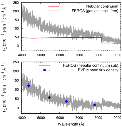
Figure 4: (upper panel) The gas-emission line free FEROS spectrum of Hen3-1357 (de-reddened, grey line) and the synthesized nebular continuum by Nebcont (red line) in the range from 4000 to 9200 Å. (lower panel) The nebular continuum subtracted FEROS spectrum (grey line) and the de-reddened $BVRIc$ band flux densities (blue circles) based on this residual FEROS spectrum.

Table 9: $BVRIc$ band de-reddened flux densities of the CSPN’s SED derived from the residual FEROS spectrum. The extinction free $V$-band magnitude ($m_{V}$) is 14.51 $\pm$ 0.17, where $F_{\lambda}$($m_{V}$ = 0) is 3.631(–9) erg s^-1 cm^-2 Å^-1.

$\lambda_{c}$ (Å)	Band	$F_{\lambda}$ (erg s-1 cm-2 Å-1)
4378.1	Johnson-$B$	1.21(–14) $\pm$ 1.14(–15)
5466.1	Johnson-$V$	5.69(–15) $\pm$ 8.76(–16)
6358.0	Cousins-$R$	3.58(–15) $\pm$ 8.66(–16)
7829.2	Cousins-$I$	1.63(–15) $\pm$ 7.08(–16)

First, we investigated the SED of the CSPN using the FEROS spectrum, which is the sum of the nebular emission lines and continuum and the CSPN spectrum. For this end, we need to subtract the nebular continuum from the FEROS spectrum. We used the Nebcont code in the Dispo package of STARLINK v.2015A to generate the nebular continuum. For the calculation, we adopted the H$\beta$ flux of the entire nebula 9.83(–12) erg s^-1 cm^-2, $n$(He⁺/H⁺) = 9.69(–2), $T_{\rm e}$ = 8090 K, and $n_{\rm e}$ = 22 860 cm^-3, which is the average among $n_{\rm e}$([S iii]), $n_{\rm e}$([Cl iii]), $n_{\rm e}$([Ne iii]), and $n_{\rm e}$([Ar iv]).

In Fig. 4 upper panel, we show the synthesized nebular continuum. The discontinuity around 8200 Å indicates the Paschen jump. After we had scaled the de-reddened FEROS spectrum up to match with the H$\beta$ line flux of the entire nebula, we manually removed gas emission lines to the extent possible. This gas emission line free FEROS spectrum is presented in the same panel. In the lower panel, we show the resultant spectrum generated by subtracting the synthesis nebular continuum spectrum from the gas emission line free and flux density scaled FEROS spectrum. Note that the residual spectrum coincides with the spectrum of the CSPN. A spike feature around 8200 Å is from the residuals of Paschen and Bracket continuum between the observed and the model. If we can subtract this continuum around Paschen jump from the observed spectrum, the spike feature will be gone. This spike feature does not affect $Ic$-band magnitude measurement. Using this residual spectrum, we measured flux densities for $BVRIc$ bands by taking filter transmission curves of each band, as summarized in Table 9.

4.2 Synthesis of the CSPN’s SED / Core-Mass / Distance

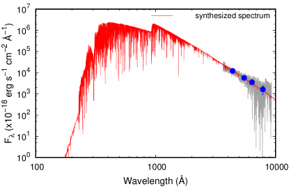
Figure 5: The spectrum of the CSPN synthesized using Tlusty (red line) in $T_{\rm eff}$ = 45 000 K and $\log\,g$ = 5.25 cm s^-2. The flux density is scaled down to the $F_{\lambda}$ = 5.69(–15) erg s^-1 cm^-2 Å^-1at 5466.1 Å. The grey line and blue circles are the same as indicated in Fig 4.

Reindl et al. (2014) performed spectral synthesis fitting of the spectrum of the CSPN taken using Far Ultraviolet Spectroscopic Explorer (FUSE) in 2006, and they obtained $T_{\rm eff}$ = 55 000 K and $\log$ $g$ = 6.0 $\pm$ 0.5 cm s^-2. However, in our Cloudy model with this $T_{\rm eff}$ and the measured de-reddened $m_{V}$ of the CSPN (14.51, see §4.1) determining the luminosity, we overproduced the fluxes of higher IP ions such as [Ne iii] and [O iii] lines.

It might be because the nebula ionization structure is not yet fully changed by the recent very fast post-AGB evolution of the CSPN. Although we firmly believe the results of Reindl et al. (2014), we needed to adopt a SED of the CSPN with a lower $T_{\rm eff}$ to reproduce the overall observed nebular line fluxes. For instance, we estimated $T_{\rm eff}$ to be 50 560 $\pm$ 2710 K using the [O iii]/H$\beta$ line ratio and the formula established among PNe in the Large Magellanic Cloud by Dopita & Meatheringham (1991).

Therefore, we utilized the non-local thermodynamic equilibrium (non-LTE) stellar atmospheres modeling code Tlusty (Hubeny, 1988) to obtain SED of the CSPN for our Cloudy model. Using Tlusty, we constructed line-blanketed, plane-parallel, and hydrostatic stellar atmosphere, where we considered the He/C/N/O/Ne/Si/P/S/Fe abundances. We run a grid model to cover $T_{\rm eff}$ from 43 000 to 53 000 K in a constant 1000 K steps. Here, we adopted the observed nebular $\epsilon$(He), $\epsilon$(N(CEL)), $\epsilon$(O(CEL)), $\epsilon$(Ne), and $\epsilon$(S). We adopted the expected $\epsilon$(C(CEL)) = 7.98 (see Table 8). As Reindl et al. (2014) reported, there is no significant difference between the nebular and stellar He/C/N/O/S abundances. We adopted stellar $\epsilon$(Si) = 7.52 and $\epsilon$(P) = 4.42 derived by Reindl et al. (2014). From the nebular $\langle$[S,Ar/H]$\rangle$ = –0.23, we adopted $\epsilon$(Fe) = 7.23. We interpret that 99 $\%$ of the Fe-atoms in the stellar atmosphere is eventually locked as dust grains in the nebula. We set the microturbulent velocity to 10 km s^-1 and the rotational velocity to 20 km s^-1.

Based on Reindl et al. (2014, 2017), Parthasarathy et al. (1993), and Karakas (2010), the core-mass of the CSPN ($m_{\ast}$) is $\sim$0.53-0.6 $M_{\sun}$. Referring to the theoretical post-AGB evolution tracks presented in Fig. 4 of Reindl et al. (2017), we adopted $\log\,g$ = 5.25 cm s^-2, and we adopted the distance $D$ = 2.5 kpc to obtain $m_{\ast}$ $\sim$0.53-0.6 $M_{\sun}$. $D$ has been determined in the range between 826 pc (see Reindl et al., 2017, reference therein) and 5.85 kpc (Frew et al., 2016), so far. When we adopt $D$ = 826 pc, we have to set a very small inner radius of the nebula to reproduce the observed H$\beta$ flux by setting a very small inner radius, we overproduced fluxes of higher IP lines and obtained hotter dust temperatures, accordingly causing lower dust continuum fluxes. If $D$ is 5.0 kpc, the situation would become better than the case of $D$ = 826 pc, and then we can reproduce the observed line fluxes. However, we have to set $\log\,g$ $\sim$4.5 cm s^-2 in order to obtain the above $m_{\ast}$ range. And Hen3-1357 would be classified as a halo PN not a thin disk PN.

We verified our adopted $D$ of 2.5 kpc. Following Quireza et al. (2007), we can classify Hen3-1357 into a Type II or III PN based on the observed $\epsilon$(He) and N/O ratio. Hen3-1357 would be a thin disk population. Quireza et al. (2007) reported that the average peculiar velocity relative to the Galaxy rotation ($\Delta$$V$) is $\sim$23 km s^-1 for Type IIb and $\sim$70 km s^-1 for Type III and the average height from the Galactic plane ($|z|$) is $\sim$0.225 kpc for Type IIa and $\sim$0.686 kpc for Type III, respectively. From the constraint on $|z|$, we obtained a range of $D$ toward Hen3-1357 between 1.07 and 3.27 kpc. Maciel & Lago (2005) calculated the rotation velocities at the nebula Galactocentric positions calculated for a Galaxy disk rotation curve based on four distance scales. Using their established Galaxy rotation velocity based on the distance scale of Cahn et al. (1992), van de Steene & Zijlstra (1995), and Zhang (1995), equation (3) of Quireza et al. (2007), and our measured LSR radial velocity 12.29 km s^-1 (see §3.3), we obtained a $D$ versus $\Delta$$V$ plot. Using this plot and the constraint on $\Delta$$V$, we got another range of $D$ between 1.63 and 4.92 kpc. Thus, we obtained $D$ = 1.63-3.27 kpc, finally. 2.5 kpc is the middle value of this distance range. From the above discussion, we adopted $D$ = 2.5 kpc and the absolute $V$-band magnitude of the CSPN $M_{V}$ = 2.555.

Finally, we obtained the synthesized spectra using SYNSPEC as displayed in Fig. 5.

4.3 Parameters of the nebular gas and dust grain

4.3.1 Nebular elemental abundances

We adopted elemental abundances listed in Table 8 as a first guess. We refined these abundances to reproduce the observed emission line intensities. For the other elements unseen in the FEROS and Spitzer/IRS spectra, we referred to the predicted values in the AGB nucleosynthesis model for initially 1.5 $M_{\sun}$ stars with $Z$ = 0.008 by Karakas (2010). For the sake of consistency, we substituted the transition probabilities and effective collision strengths of CELs by the same values applied in our nebular abundance analysis.

In spite of non-detection in the Spitzer/IRS spectrum, our Cloudy model with the AGB nucleosynthesis predicted $\epsilon$(Si) overestimated the $[$Si iii$]$ 34.82 µm line. This indicates that most of the Si-atoms exist as amorphous silicate dust grains. Therefore, we took care of the Si and Mg abundances as silicate grain components. Assuming that the nebular [Mg,Si/H] is comparable to the [Mg/H] = –1.69 measured in the PN IC4846 (Hyung et al., 2001), we kept $\epsilon$(Mg) = 5.86 and $\epsilon$(Si) = 5.84, respectively. As we discussed later, IC4846 displays amorphous silicate features (e.g., Stanghellini et al., 2012) and very similar elemental abundances to Hen3-1357.

4.3.2 Nebula geometry/boundary condition/gas filling factor

We adopted spherical shell with a uniform hydrogen density. We assumed the ionization boundary radius ($r_{\rm ib}$) of $\sim$1.3″ using a plot of count versus size of the circular aperture generated by the archival HST/Wide Field Planetary Camera 2 (WFPC2) F487N (H$\beta$) image taken on 1996 March 3 (Prop-ID: GO6039, PI: M. Bobrowsky). 85 % of the total count is measured within 1.28″. Although the exact size of the nebula in 2006 is unknown, slow nebula shell expansion velocity suggests that the size of the nebula is not largely different since 1996. Here, we measured twice expansion velocities (2$V_{\rm exp}$) using equation (3) of Otsuka et al. (e.g., 2003, 2009, 2015) and 144 emission lines as summarized in appendix Table A5. To calculate line broadening by gas thermal motion, we adopted suitable $T_{\rm e}$ for each ion by referring to Table 4. In Hen3-1357, 2$V_{\rm exp}$ did not correlate with IP. We measured the average 2$V_{\rm exp}$ = 14.8 $\pm$ 0.5 km s^-1 among the 39 H i lines, which is consistent with the mean expansion velocity ($V_{\rm exp}$) of 8.4 $\pm$ 1.5 km s^-1 measured from the 17 lines by Arkhipova et al. (2013).

Filling factor $f$ can be defined as the ratio of an RMS density derived from a hydrogen line flux, $T_{\rm e}$, and nebula radius to the $n_{\rm e}$(CELs) (see, e.g., Mallik & Peimbert, 1988; Peimbert et al., 2000). We calculated an RMS density of 10 750 cm^-3 from the H$\beta$ flux of the entire nebula, $T_{\rm e}$ = 8 060 K, $r_{\rm ib}$ = 1.28″, and a constant $n_{\rm e}$/$n({\rm H^{+}})$ = 1.15. We estimated $f$ to be 0.47-0.62 using this RMS density and the observed $n_{\rm e}$(CELs). Here, we set $f$ = 0.55 as a first guess and varied.

4.3.3 Dust grains and size distribution

We assumed spherical shaped silicate grain and adopted a standard interstellar size distribution ($n(a)\propto a^{-3.5}$, Mathis et al., 1977) with radius $a$ = 0.01-0.50 µm. We selected the dielectric function table of astronomical silicate currently recommended by the webpage of B. Draine .

4.4 Model result

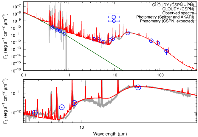
Figure 6: (upper panel) Comparison between the Cloudy model and observational data of Hen3-1357. The blue diamonds indicate the observed $BVRIc$ band flux densities of the CSPN, which are the same values in listed in Table 9. (lower panel) Closed-up plots in 5-40 µm. In both panels, we set the spectral resolution of the synthesized Cloudy spectrum to be a constant 600, corresponding to that of Spitzer/IRS SH and LH spectra.

Table 10: The best-fit Cloudy model parameters of Hen3-1357.

Parameters of the CSPN	Value
$L_{\ast}$ / $T_{\rm eff}$ / $\log\,g$ / $D$	330 $L_{\sun}$ / 45 550 K / 5.25 cm s-2 / 2.5 kpc
$M_{V}$	2.555
$R_{\ast}$	0.291 $R_{\sun}$
$m_{\ast}$	0.550 $M_{\sun}$
Parameters of the Nebula	Value
$\epsilon$(X)	He:10.97, C:8.18, N:7.89, O:8.58, Ne:8.20
	Mg:5.86, Si:5.84, S:6.74, Cl:4.73, Ar:6.25
	Fe:5.23, Others: Karakas (2010)
Geometry	Spherical symmetry
Shell size	$r_{\rm in}$:0.44″ (0.005 pc), $r_{\rm out}$:2.77″ (0.034 pc)
Ionization boundary	1.48″ (0.018 pc)
radius ($r_{\rm ib}$)
Filling factor ($f$)	0.58
$n_{\rm H}$	11 610 cm-3
$F$(H$\beta$)	9.84(–12) erg s-1 cm-2 (de-reddened)
$m_{g}$	3.81(–2) $M_{\sun}$
Parameters of the Dust	Value
Grain size	0.01-0.50 µm
$T_{d}$	40-150 K
$m_{d}$	1.98(–4) $M_{\sun}$
$m_{d}$/$m_{g}$ (DGR)	5.20(–3)

Table 11: Comparison of the ICFs between the observation and the Cloudy model.

Elem.	ICF(obs)	ICF(model)
He	1.00	1.03
C(RL)	1.48 $\pm$ 0.22	1.30
N(RL)	1.48 $\pm$ 0.22	1.62
N(CEL)	3.09 $\pm$ 0.17	2.69
O(RL)	2.45 $\pm$ 0.07	2.23
O(CEL)	1.00	1.04
Ne	1.00	1.01
S	1.00	1.00
Cl	1.01 $\pm$ 0.06	1.01
Ar	1.00	1.01
Fe	2.30 $\pm$ 0.14	2.07

To find the best-fit model, we varied $T_{\rm eff}$, the inner radius of the nebula $r_{\rm in}$, $n_{\rm H}$, $\epsilon$(He/C/N/O/Ne/S/Cl/Ar/Fe), dust mass fraction, and $f$ within a given range by using the optimize command available in Cloudy.

García-Hernández et al. (2002) found that the distribution of molecular hydrogen H₂ $v$=1-0 S(1) at 2.122 µm and $v$=2-1S (1) at 2.248 µm is quite homogeneous and extends well beyond the distribution of the H i Br$\gamma$ line. This suggests that Hen3-1357 has large neutral regions.

Thus, we went to deep neutral gas regions in our model; we continued calculation until any of the model’s predicted flux densities at AKARI/FIS 65/90/140 µm bands reached or exceeded the relevant observed values. Cloudy model predicted $r_{\rm ib}$ = 1.48″ where $T_{\rm e}$ drops below 4000 K. We stopped model calculation at the outer radius ($r_{\rm out}$) of 3.4(–2) pc (2.77″). The goodness of fit was determined by the reduced $\chi^{2}$ value calculated from the following observational constraints: 17 broadband fluxes, 5 broadband flux densities, 104 gas emission fluxes, $r_{\rm ib}$, de-redden $F$(H$\beta$) of the entire nebula. Table 10 summarizes the parameters of the best-fit model, where the reduced $\chi^{2}$ is 33.5.

The SED of the best-fit model, in comparison with the observational data is presented in Fig. 6. From the model result, we confirmed that gas emission contribution to Spitzer/IRAC 8.0 µm and AKARI/IRC 9.0/18 µm bands is 51.8 %, 19.1 %, and 3.9 %, respectively. Thus, the disagreement at Spitzer/IRAC 8.0 µm band between the observed photometry and the predicted SED can be explained by considering the gas emission contribution to the relevant band.

The observed and model predicted line fluxes, band fluxes, and band flux densities are summarized in appendix Table A6. The intensity of the O ii 4075 Å and 4651 Å is the sum of the multiplet V10 and V1 O ii lines, respectively. It is noteworthy that we simultaneously reproduced both the observed RL/CEL N and O line fluxes.

The predicted ICF(X) by Cloudy listed in Table 11 is in excellent agreement with the ICF(X) derived in §3.7, indicating that our Cloudy model succeeded to explain ionization nebula structure and the ICF(X) based on IP is proper value.

As described in §4.2, under the constraints to the CSPN at $D$ = 2.5 kpc, we need $T_{\rm eff}$ = 45 550 K and $L_{\ast}$ = 330 $L_{\odot}$ in order to explain the observed quantities. With $D$, $L_{\ast}$, and $\log\,g$, we derived $m_{\ast}$ = 0.55 $M_{\odot}$.

The gas mass ($m_{g}$) = 3.81(–2) $M_{\sun}$ is the sum of the ionized and neutral gas masses. The ionized gas mass is 5.38(–3) $M_{\sun}$ and the remaining is the neutral gas mass. Our derived $m_{g}$ is close to the ejected mass = 8.9(–2) $M_{\odot}$ in initially 1.5 $M_{\odot}$ stars with $Z$ = 0.008 during the last thermal pulse AGB, predicted by Karakas & Lattanzio (2007). We obtained the dust mass ($m_{d}$) of 1.98(–4) $M_{\sun}$.

It is of interest to know how far-IR data impact gas and dust mass estimates in our model. When we stopped model calculation at $r_{\rm ib}$, we obtained $m_{g}$ = 4.61(–3) $M_{\sun}$ and $m_{d}$ = 3.79(–5) $M_{\sun}$, respectively. This model did not well fit any AKARI far-IR fluxes. To fit the observed far-IR data, we need a larger $r_{\rm out}$. With the AKARI far-IR data, we obviously obtained much greater $m_{g}$ and $m_{d}$. About 80 $\%$ of the total dust mass is from warm-cold dust components beyond ionization front. From the model result, we confirmed that the gas emission contribution to AKARI 65/90/140 µm bands is 1.4 %, 1.08 %, and 2.58 %, respectively. AKARI far-IR data would be thermal emission from warm-cold dust.

Cox et al. (2011) derived an upper limit of the sum of $m_{d}$ and $m_{g}$ = 0.16 $M_{\sun}$ within a 3 pc radius using the AKARI/90 µm and a constant dust-to-gas mass ratio (DGR) = 6.25(–3) for O-rich dust, although the measured dust temperature ($T_{d}$) is unknown. Using their results, we calculated an upper limit $m_{g}$ = 0.159 $M_{\sun}$ and $m_{d}$ = 9.94(–4) $M_{\sun}$, respectively.

Umana et al. (2008) derived the total ionized mass of $\sim$5.7(–2) $M_{\sun}$ using the radio data in 2002, assuming $D$ = 5.6 kpc, inner/outer radii = 0.65″/1.3″ shallow shell geometry, and $f$ = 1.0. Using the IRAS data, they derived $T_{d}$ = 137 $\pm$ 2 K, and $m_{d}$ = 2(–4) $M_{\sun}$ using the 60 µm flux density in the case of silicate. Based on the results and assumptions of Umana et al. (2008), ionized gas and co-existing dust would be $\sim$6.6(–3) $M_{\sun}$ and $\sim$4.0(–5) $M_{\sun}$, respectively if we adopt $D$ = 2.5 kpc and $f$ = 0.58. These estimated values are consistent with our derived $m_{g}$ and $m_{d}$ when we stopped the model at $r_{\rm ib}$. On the dust, Cox et al. (2011) found that the AKARI far-IR flux densities are by a factor two lower than predicted from the IRAS data. They interpreted that the far-IR variability in its infrared flux might occur due to recent mass-loss event(s) or evolution of the CSPN. Following the report of Cox et al. (2011) and the dust mass $\sim$4.0(–5) $M_{\sun}$ co-existing with the ionized gas by the IRAS data in 1980s, we estimate the dust mass to be $\lesssim$ 2(–5) $M_{\sun}$ in 2006-2007, which is comparable to our derived dust mass of 3.79(–5) $M_{\sun}$ within the ionized gas.

5 Discussion

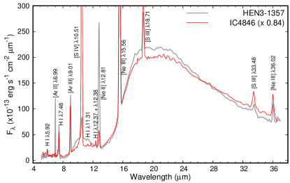
Figure 7: The Spitzer/IRS spectra of IC4846 and Hen3-1357. The spectral resolution of Hen3-1357 is down to match with that of IC4846. For IC4846, we scaled the flux density up to match with AKARI/IRC 9.0/18 µm bands (0.1311 and 2.038 Jy, respectively, Yamamura et al., 2010). For demonstration, the flux density of this scaled spectrum is further scaled to match with the IRS spectrum of Hen3-1357 by a constant factor of 0.84. See text for details.

Table 12: Comparisons with the $\epsilon$(X) of IC4846 and the average $\epsilon$(X) value among Galactic amorphous silicate rich PNe. The $\epsilon$(X) of Hen3-1357 is the result by using the ICFs, except for the CEL C, which is an expected value.

Elem.	OD PN	IC4846						Hen
(X)	Ave.	(a)	(b)	(c)	(d)	(e)	Ave.	3-1357
He	11.02	10.98	10.96	10.90	11.01	$\cdots$	10.96	10.99
C(RL)	$\cdots$	7.74	8.37	8.43	$\cdots$	$\cdots$	8.27	8.16
C(CEL)	$\cdots$	7.68	8.45	8.16	$\cdots$	7.95	8.15	7.98
N(RL)	$\cdots$	$\cdots$	$\cdots$	8.10	$\cdots$	$\cdots$	8.10	8.01
N(CEL)	7.78	7.89	7.81	8.09	7.69	$\cdots$	7.90	8.05
O(RL)	$\cdots$	$\cdots$	8.97	8.78		$\cdots$	8.89	8.84
O(CEL)	8.42	8.60	8.51	8.59	8.60	8.50	8.56	8.66
Ne	7.78	7.90	7.83	7.77	7.99	$\cdots$	7.88	8.19
Mg	$\cdots$	5.86	$\cdots$	$\cdots$	$\cdots$	$\cdots$	5.86	$\cdots$
S	6.50	6.95	6.63	7.01	6.73	$\cdots$	6.86	6.83
Cl	6.15	5.11	$\cdots$	5.34	6.14	$\cdots$	5.76	5.08
Ar	6.03	6.18	5.96	6.02	6.13	$\cdots$	6.08	6.37
Fe	$\cdots$	$\cdots$	$\cdots$	$\cdots$	$\cdots$	5.21	5.21	5.22

It is necessary to verify whether the gas and dust chemistry in Hen3-1357 is consistent with other O-rich gas and dust Galactic PNe. To compare with such PNe is an important step to understand the evolution of Hen3-1357.

García-Hernández & Górny (2014) investigated relations among dust features, elemental abundances, and evolution of the progenitors. In the second column of Table 12, we list the average $\epsilon$(X) among their amorphous silicate PNe. They found that $\epsilon$(He) and N/O ratio in these amorphous silicate containing PNe are in agreement with the AGB nucleosynthesis model predictions for initially $\sim$1.0 $M_{\sun}$ stars with $Z$ = 0.008. García-Hernández & Górny (2014) suggested that the higher Ne/O ratios in O-rich dust PNe relative to the AGB models may reflect the effect of PMZ. The observed $\epsilon$(He) and the CEL N/O ratio of 0.24 $\pm$ 0.02 in Hen3-1357 coincide with the average values in their amorphous silicate PN sample. As discussed in §3.9, our predicted progenitor mass, initial metallicity, and interpretation for the Ne overabundance in Hen3-1357 follow their results.

We can now understand relations among dust features, nebular abundances, and the progenitor stars’ evolution. Moreover, we know that the nebula morphology is connected to the central star’s evolution. Using the HST/WFPC images as a guide, we tried to find objects showing similar nebula shape, dust features, and elemental abundance pattern to Hen3-1357. As far as our best knowledge, a point-symmetric PN IC4846 (e.g., Miranda et al., 2001) is very similar to Hen3-1357.

IC4846 clearly shows amorphous silicate features as reported by Stanghellini et al. (2012). We reduced the BCD of IC4846 (obs AORKEY: 25839616, PI: L. Stanghellini) by the same process applied for Hen3-1357. In Fig. 7, we display the Spitzer/IRS spectra of IC4846 and Hen3-1357. The dust features seen in both PNe are very similar except for the different strengths of the 9 and 18 $\mu$m emission bumps, which might reflect the difference in the grain composition. For IC4846, Stasińska & Szczerba (1999) derived a single $T_{d}$ = 107 K and DGR = 1.2(–3) based on the IRAS four band fluxes using a modified blackbody function. Tajitsu & Tamura (1998) and derived a single $T_{d}$ = 168 K using the IRAS data. Zhang & Kwok (1991) derived a single $T_{d}$ = 152 K and $T_{\rm eff}$ = 47 600 K by fitting SED from IUE to IRAS data.

In the third to seventh columns of Table 12, we compile nebular abundances of IC4846 measured by prior works. The eighth column gives the average value. Obviously, the abundances in both IC4846 and Hen3-1357 are in excellent agreement even in the RL $\epsilon$(C,N,O) and the Fe-depletion. So far, the $\epsilon$(Mg) and $\epsilon$(Fe) measurements have been performed only by Hyung et al. (2001) using the IUE UV-spectrum and only by Delgado-Inglada & Rodríguez (2014) using the optical spectra, respectively. The largely depleted [Mg/H] = –1.69 in IC4846 might indicate that most of the Mg-atoms are captured by silicate grains. We assumed the similar situation to Hen3-1357 in our Cloudy model.

Hyung et al. (2001) succeeded to reproduce UV-optical gas emission line fluxes in photoionization model of IC4846 by setting the CSPN’s radius 0.425 $R_{\sun}$, $T_{\rm eff}$ = 70 000 K, $\log\,g$ = 4.6 cm s^-2, and $D$ = 7 kpc, which give $L_{\ast}$ = 3900 $L_{\sun}$. With comparison with post-AGB evolutionary tracks, they estimated $m_{\ast}$ $\sim$0.57 $M_{\sun}$.

From above comparisons, we can conclude that Hen3-1357 is an ordinary amorphous silicate rich and O-rich gas PN. Among amorphous silicate rich PNe in the Milky Way, IC4846 is very similar to Hen3-1357. Both PNe have evolved from similar progenitor mass stars with $Z$ = 0.008. However, the rapid evolution of the central star of Hen3-357 still remains a puzzle.

6 Summary

We performed a detailed chemical abundance analysis and constructed the photoionization model of Hen3-1357 to characterize the PN and obtain a coherent picture of the dusty nebula and CSPN in 2006 based on optical to far-IR data.

We calculated the abundances of the nine elements. The RL C/O ratio indicates that Hen3-1357 is an O-rich PN, supported by the detection of the broad 9/18 $\mu$m amorphous silicate bands in the Spitzer/IRS spectrum. The ADF(O²⁺) is less than a typical value measured in PNe. The observed elemental abundances can be explained by AGB nucleosynthesis models of Karakas (2010) for initially 1-1.5 $M_{\odot}$ stars with $Z$ = 0.008. The Ne overabundance might be due to the enhancement of ²²Ne isotope in the He-rich intershell.

We did not find significant variation of nebular line intensities between 2006 and 2011, suggesting that nebular ionization state and elemental abundances are most likely in a steady state during the same period, while the central star is rapidly evolving.

By incorporating the spectrum of the CSPN synthesized by Tlusty as the ionization/heating source of the PN with Cloudy modeling, we succeeded to explain the observed SED and derive the gas and dust masses, dust-to-gas mass ratio, and core-mass of the CSPN. About 80 % of the total dust mass is from the warm-cold dust components beyond ionization front.

Through comparison with other Galactic PNe, we found that Hen3-1357 is an ordinary amorphous silicate rich and O-rich gas PN. IC4846 shows many similarities in properties of the PN to Hen3-1357.

Although we derived physical properties of the nebula and also provided the range of the progenitor mass, the rapid evolution from post-AGB B1 supergiant in 1971 to a young PN in a matter of 21 years is not yet understood. If the central star has experienced LTP then it should be H-poor, He and C-rich in its present hot post-AGB stage soon after the LTP. However, the nebular and stellar chemical compositions calculated by us and Reindl et al. (2014, 2017) are nearly solar, not at all similar to those of LTP PNe. If the central star has now started returning towards the AGB phase, then very soon it will go through A, F, and G spectral types before it appears as a born-again AGB star. If so, it may show abundances similar to that of LTP PN in future. We need to monitor the central star’s $T_{\rm eff}$, $\log\,g$, and chemical composition in order to confirm whether it is evolving back towards the AGB stage. If Hen3-1357 is a binary, rapid evolution might be explained. For that end, monitoring of radial velocity using stellar absorption profiles in UV wavelength would be necessary. Moreover, comparisons with other Galactic amorphous silicate rich and O-rich gas PNe such as IC4846 can help us to understand the evolution of Hen3-1357. Thus, further observations of both the nebula and the central star are required for further understanding this PN.

Table 1: The identified atomic emission lines in the FEROS spectrum. The first column is the wavelength at the observation. The third column is the wavelength at rest in laboratory.

$\lambda_{\rm obs.}$	Line	$\lambda_{\rm lab.}$	$f$($\lambda$)	$I$($\lambda$)	$\delta$$I$($\lambda$)
(Å)		(Å)		($I$(H$\beta$) = 100)
3697.33	H i (B17)	3697.15	0.328	1.923	0.107
3704.01	H i (B16)	3703.85	0.327	2.028	0.122
3705.16	He i	3704.98	0.327	0.965	0.087
3712.12	H i (B15)	3711.97	0.325	2.384	0.119
3722.02	H i (B14)	3721.94	0.323	4.156	0.155
3723.81	Fe ii]	3723.92	0.323	0.474	0.058
3726.20	[O ii]	3726.03	0.322	101.210	2.625
3728.96	[O ii]	3728.81	0.322	37.647	0.979
3734.52	H i (B13)	3734.37	0.321	3.026	0.097
3750.31	H i (B12)	3750.15	0.317	4.220	0.124
3770.79	H i (B11)	3770.63	0.313	4.353	0.115
3798.05	H i (B10)	3797.90	0.307	5.330	0.133
3819.79	He i	3819.60	0.302	1.142	0.033
3833.75	He i	3833.55	0.299	0.072	0.010
3835.54	H i (B9)	3835.38	0.299	7.597	0.183
3867.69	He i	3867.47	0.291	0.147	0.008
3868.92	[Ne iii]	3869.06	0.291	40.325	0.946
3871.95	He i	3871.79	0.290	0.078	0.006
3889.06	H i (B8)	3889.05	0.286	15.997	0.472
3926.71	He i	3926.54	0.277	0.124	0.005
3964.90	He i	3964.73	0.267	0.540	0.012
3967.63	[Ne iii]	3967.79	0.267	10.000	0.216
3970.23	H i (B7)	3970.07	0.266	16.026	0.341
4009.42	He i	4009.26	0.256	0.152	0.006
4026.37	He i	4026.20	0.251	1.532	0.031
4068.77	[S ii]	4068.60	0.239	4.471	0.086
4069.74	O ii	4069.62	0.239	0.027	0.003
4070.04	O ii	4069.88	0.239	0.038	0.005
4072.32	O ii	4072.15	0.238	0.057	0.003
4076.02	O ii	4075.86	0.237	0.076	0.005
4076.52	[S ii]	4076.35	0.237	1.508	0.029
4097.45	N iii	4097.35	0.231	0.023	0.003
4101.90	H i (B6, H$\delta$)	4101.73	0.230	21.516	0.395
4103.19	O ii	4103.00	0.229	0.030	0.004
4103.81	N iii	4103.39	0.229	0.028	0.004
4105.13	O ii	4104.99	0.229	0.040	0.004
4119.45	O ii	4119.22	0.224	0.019	0.004
4121.00	He i	4120.81	0.224	0.177	0.005
4143.93	He i	4143.76	0.217	0.229	0.005
4153.44	O ii	4153.30	0.214	0.031	0.002
4267.35	C ii	4267.18	0.180	0.103	0.005
4276.00	O ii	4275.99	0.177	0.032	0.005
4340.64	H i (B5, H$\gamma$)	4340.46	0.157	46.052	0.579
4349.64	O ii	4349.43	0.154	0.033	0.002
4363.38	[O iii]	4363.21	0.149	2.461	0.030
4367.08	O ii	4366.90	0.148	0.034	0.003
4368.41	O i	4368.24	0.148	0.036	0.002
4388.11	He i	4387.93	0.142	0.439	0.006
4437.76	He i	4437.55	0.126	0.066	0.004
4471.68	He i	4471.47	0.115	4.628	0.048
4591.14	N ii	4590.85	0.078	0.036	0.005
4630.71	N ii	4630.54	0.066	0.020	0.003
4639.02	O ii	4638.86	0.064	0.034	0.004
4642.01	O ii	4641.81	0.063	0.064	0.002
4649.33	O ii	4649.13	0.061	0.103	0.003
4651.01	O ii	4650.84	0.060	0.034	0.002
4658.33	[Fe iii]	4658.05	0.058	0.111	0.002
4661.83	O ii	4661.63	0.057	0.048	0.002
4676.48	O ii	4676.23	0.053	0.032	0.005
4701.86	[Fe iii]	4701.53	0.045	0.046	0.003
4711.59	[Ar iv]	4711.37	0.042	0.034	0.003
4713.38	He i	4713.22	0.042	0.668	0.007
4725.73	[Ne iv]?	4725.64	0.038	0.011	0.002
4734.06	[Fe iii]	4733.91	0.036	0.026	0.003
4740.41	[Ar iv]	4740.16	0.034	0.070	0.002
4754.94	[Fe iii]	4754.69	0.030	0.029	0.004
4861.52	H i (B4, H$\beta$)	4861.33	0.000	100.000	0.112
4881.20	[Fe iii]	4881.00	-0.005	0.045	0.004
4891.21	O ii?	4890.86	-0.008	0.032	0.008
4922.13	He i	4921.93	-0.016	1.214	0.004
4924.78	[Fe iii]	4924.54	-0.017	0.027	0.002
4931.45	[O iii]	4931.23	-0.019	0.055	0.003
4959.13	[O iii]	4958.91	-0.026	145.519	0.380
4987.58	[Fe iii]	4987.21	-0.033	0.016	0.003
4996.95	O ii	4996.98	-0.035	0.045	0.004
5015.88	He i	5015.68	-0.040	2.161	0.012
5047.95	He i	5047.74	-0.048	0.168	0.003
5146.79	[Fe iii]	5146.45	-0.071	0.027	0.004
5159.01	[Fe ii]	5158.78	-0.074	0.017	0.002
5191.94	[Ar iii]	5191.82	-0.081	0.064	0.003
5198.13	[N i]	5197.90	-0.082	0.363	0.004
5200.49	[N i]	5200.26	-0.083	0.228	0.004
5270.74	[Fe iii]	5270.40	-0.098	0.059	0.002
5517.91	[Cl iii]	5517.72	-0.145	0.117	0.003
5538.06	[Cl iii]	5537.89	-0.149	0.240	0.005
5577.64	[O i]	5577.34	-0.156	0.219	0.004
5679.81	N ii	5679.56	-0.173	0.017	0.002
5754.83	[N ii]	5754.64	-0.185	2.578	0.038
5791.58	C ii	5791.69	-0.190	0.021	0.002
5875.88	He i	5875.60	-0.203	14.666	0.262
5958.74	O i	5958.54	-0.215	0.026	0.004
6300.55	[O i]	6300.30	-0.263	16.129	0.339
6312.32	[S iii]	6312.10	-0.264	1.031	0.022
6364.04	[O i]	6363.78	-0.271	5.095	0.111
6527.42	[N ii]	6527.24	-0.293	0.019	0.003
6548.32	[N ii]	6548.04	-0.296	40.956	0.967
6578.31	C ii	6578.05	-0.300	0.050	0.004
6583.70	[N ii]	6583.46	-0.300	121.454	2.915
6678.42	He i	6678.15	-0.313	3.972	0.099
6716.73	[S ii]	6716.44	-0.318	6.066	0.154
6721.76	O ii	6721.39	-0.319	0.009	0.002
6731.10	[S ii]	6730.81	-0.320	12.471	0.319
7002.42	O  i	7002.12	-0.356	0.051	0.004
7062.57	He i	7062.28	-0.364	0.019	0.003
7065.50	He i	7065.18	-0.364	7.846	0.247
7136.06	[Ar iii]	7135.80	-0.374	10.767	0.322
7155.53	[Fe ii]	7155.16	-0.376	0.034	0.003
7160.85	He i	7160.61	-0.377	0.027	0.003
7254.70	O  i	7254.45	-0.390	0.064	0.004
7281.64	He i	7281.35	-0.393	0.726	0.023
7298.33	He i	7298.04	-0.395	0.035	0.003
7319.33	[O ii]	7318.92	-0.398	3.998	0.130
7320.40	[O ii]	7319.99	-0.398	13.487	0.430
7329.96	[O ii]	7329.66	-0.400	7.476	0.239
7331.04	[O ii]	7330.73	-0.400	6.987	0.224
7378.30	[Ni ii]	7377.83	-0.406	0.030	0.003
7500.18	He i	7499.85	-0.422	0.036	0.004
7751.42	[Ar iii]	7751.10	-0.455	2.630	0.096
7816.45	He i	7816.14	-0.464	0.077	0.003
8245.95	H i (P42)	8245.64	-0.516	0.033	0.004
8248.09	H i (P41)	8247.73	-0.516	0.027	0.003
8250.17	H i (P40)	8249.97	-0.517	0.028	0.001
8252.65	H i (P39)	8252.40	-0.517	0.033	0.002
8255.36	H i (P38)	8255.02	-0.517	0.027	0.002
8258.21	H i (P37)	8257.85	-0.517	0.041	0.002
8261.20	H i (P36)	8260.93	-0.518	0.042	0.002
8264.69	He i	8264.62	-0.518	0.059	0.003
8268.31	H i (P34)	8267.94	-0.519	0.055	0.003
8272.22	H i (P33)	8271.93	-0.519	0.057	0.003
8276.60	H i (P32)	8276.31	-0.520	0.070	0.004
8281.49	H i (P31)	8281.12	-0.520	0.072	0.004
8286.71	H i (P30)	8286.43	-0.521	0.111	0.005
8292.67	H i (P29)	8292.31	-0.521	0.096	0.005
8299.20	H i (P28)	8298.83	-0.522	0.118	0.005
8306.48	H i (P27)	8306.11	-0.523	0.119	0.005
8314.61	H i (P26)	8314.26	-0.524	0.128	0.006
8323.76	H i (P25)	8323.42	-0.525	0.143	0.006
8334.11	H i (P24)	8333.78	-0.526	0.152	0.007
8342.74	C iii	8342.20	-0.527	0.020	0.002
8345.85	H i (P23)	8345.55	-0.527	0.188	0.008
8359.31	H i (P22)	8359.00	-0.529	0.220	0.009
8362.07	He i	8361.73	-0.529	0.082	0.004
8374.81	H i (P21)	8374.48	-0.531	0.219	0.009
8392.73	H i (P20)	8392.40	-0.533	0.252	0.011
8397.80	He i	8397.42	-0.533	0.010	0.001
8413.65	H i (P19)	8413.32	-0.535	0.288	0.012
8434.02	[Cl iii]	8434.00	-0.537	0.008	0.001
8438.29	H i (P18)	8437.95	-0.537	0.326	0.014
8444.79	He i	8444.55	-0.538	0.025	0.003
8446.82	O  i	8446.48	-0.538	0.468	0.020
8451.52	He i	8451.17	-0.539	0.013	0.003
8467.58	H i (P17)	8467.25	-0.541	0.378	0.016
8486.63	He i	8480.79	-0.543	0.017	0.002
8500.45	[Cl iii]	8500.20	-0.544	0.010	0.004
8502.82	H i (P16)	8502.48	-0.544	0.450	0.020
8545.71	H i (P15)	8545.38	-0.549	0.508	0.023
8579.06	[Cl ii]	8578.69	-0.552	0.304	0.014
8582.21	He i	8581.88	-0.552	0.024	0.003
8598.73	H i (P14)	8598.39	-0.554	0.636	0.028
8617.23	[Fe ii]	8616.95	-0.556	0.042	0.002
8648.62	He i	8648.26	-0.559	0.030	0.002
8665.37	H i (P13)	8665.02	-0.560	0.829	0.037
8680.62	N i	8680.28	-0.562	0.017	0.001
8683.85	N i	8683.40	-0.562	0.017	0.001
8703.64	N i	8703.25	-0.564	0.012	0.001
8727.55	[C i]	8727.12	-0.566	0.014	0.002
8733.82	He i	8733.44	-0.567	0.037	0.003
8736.36	He i	8736.04	-0.567	0.012	0.002
8750.82	H i (P12)	8750.47	-0.568	1.042	0.047
8777.05	He i	8776.83	-0.571	0.053	0.003
8845.72	He i	8845.39	-0.576	0.055	0.004
8892.21	[Fe ii]	8891.91	-0.580	0.016	0.002
8997.34	He i	8997.00	-0.588	0.055	0.004
9000.05	He i	8999.75	-0.589	0.022	0.002
9015.29	H i (P10)	9014.91	-0.590	1.624	0.077
9052.33	[Fe ii]	9051.95	-0.592	0.011	0.002
9063.71	He i	9063.32	-0.593	0.060	0.004
9069.29	[S iii]	9068.60	-0.594	12.577	0.596
9123.99	[Cl ii]	9123.60	-0.598	0.103	0.005
9210.69	He i	9210.34	-0.604	0.099	0.006

References. — The average abundance of Galactic amorphous silicate rich PNe in the Galaxy (OD PN Ave) in the second column is taken from García-Hernández & Górny (2014). On elemental abundances of the PN IC4846 in the third - seventh columns - (a) Hyung et al. (2001), (b) Wesson et al. (2005), (c) Wang & Liu (2007), (d) García-Hernández & Górny (2014), and (e) Delgado-Inglada & Rodríguez (2014). The eighth column is the average among the measurements by (a)-(e).

Table A2: The identified lines in the Spitzer/IRS spectrum. The flux density is scaled-up to match with the AKARI/IRC 9.0 µm band flux density. Then, the fluxes of these identified atomic lines are normalized with respect to the H$\beta$ flux of the entire nebula 9.83(–12) $\pm$ 7.33(–13) erg s^-1 cm^-2. See text in details.

$\lambda_{\rm lab.}$	Line	$I$($\lambda$)
($\micron$)		($I$(H$\beta$) = 100)
$5.92$	H i	$0.740~{}\pm~{}0.042$
$6.99$	$[$Ar ii$]$	$7.435~{}\pm~{}0.253$
$7.48$	H i	$6.186~{}\pm~{}0.223$
$9.01$	$[$Ar iii$]$	$12.993~{}\pm~{}0.471$
$10.51$	$[$S iv$]$	$7.758~{}\pm~{}0.266$
$11.31$	H i	$0.277~{}\pm~{}0.068$
$12.37$	H i	$1.043~{}\pm~{}0.034$
$12.81$	$[$Ne ii$]$	$46.711~{}\pm~{}1.553$
$14.37$	$[$Cl ii$]$?	$0.323~{}\pm~{}0.040$
$15.56$	$[$Ne iii$]$	$96.699~{}\pm~{}3.188$
$17.62$	He i?	$1.274~{}\pm~{}0.094$
$18.71$	$[$S iii$]$	$13.864~{}\pm~{}0.465$
$33.48$	$[$S iii$]$	$3.517~{}\pm~{}0.272$
$36.02$	$[$Ne iii$]$	$6.180~{}\pm~{}0.323$

Table A3: Comparison of the overlapped line fluxes between our 2006 and Arkhipova et al. (2013)’s 2011 observations. $F$($\lambda$) and $I$($\lambda$) are normalized to the $F$(H$\beta$) and $I$(H$\beta$), where are 100, respectively.

$\lambda_{\rm lab.}$ (Å)	Line	$F$($\lambda$) in 2006	$F$($\lambda$) in 2011	$I$($\lambda$) in 2006	$I$($\lambda$) in 2011
3726/29	[O ii]	$130.595~{}\pm~{}0.345$	$126.8~{}\pm~{}7.2$	$138.857~{}\pm~{}2.801$	$163.0~{}\pm~{}9.5$
4101.73	B6	$20.596~{}\pm~{}0.031$	$18.4~{}\pm~{}2.5$	$21.516~{}\pm~{}0.395$	$21.6~{}\pm~{}2.9$
4340.46	B5	$44.700~{}\pm~{}0.067$	$45.8~{}\pm~{}2.2$	$46.052~{}\pm~{}0.579$	$50.9~{}\pm~{}2.5$
4363.21	[O iii]	$2.392~{}\pm~{}0.004$	$4.1~{}\pm~{}1.6$	$2.461~{}\pm~{}0.030$	$4.6~{}\pm~{}1.8$
4958.91	[O iii]	$146.232~{}\pm~{}0.237$	$150.8~{}\pm~{}3.8$	$145.519~{}\pm~{}0.380$	$148.0~{}\pm~{}3.8$
5754.64	[N ii]	$2.671~{}\pm~{}0.006$	$3.9~{}\pm~{}1.1$	$2.578~{}\pm~{}0.038$	$3.3~{}\pm~{}0.9$
5875.60	He i	$15.244~{}\pm~{}0.115$	$18.1~{}\pm~{}0.9$	$14.666~{}\pm~{}0.262$	$15.2~{}\pm~{}0.7$
6300.30	[O i]	$16.956~{}\pm~{}0.021$	$22.5~{}\pm~{}0.9$	$16.129~{}\pm~{}0.339$	$17.7~{}\pm~{}0.7$
6312.10	[S iii]	$1.084~{}\pm~{}0.003$	$1.6~{}\pm~{}0.5$	$1.031~{}\pm~{}0.022$	$1.2~{}\pm~{}0.4$
6363.78	[O i]	$5.365~{}\pm~{}0.09$	$8.3~{}\pm~{}0.7$	$5.095~{}\pm~{}0.111$	$6.5~{}\pm~{}0.6$
6548.04	[N ii]	$43.327~{}\pm~{}0.054$	$60.9~{}\pm~{}1.6$	$40.956~{}\pm~{}0.967$	$46.5~{}\pm~{}1.3$
6583.46	[N ii]	$128.601~{}\pm~{}0.168$	$190.2~{}\pm~{}5.1$	$121.454~{}\pm~{}2.915$	$144.6~{}\pm~{}4.2$
6678.15	He i	$4.215~{}\pm~{}0.007$	$5.6~{}\pm~{}0.8$	$3.972~{}\pm~{}0.099$	$4.2~{}\pm~{}0.6$
6716.44	[S ii]	$6.444~{}\pm~{}0.010$	$11.3~{}\pm~{}0.9$	$6.066~{}\pm~{}0.154$	$8.5~{}\pm~{}0.6$
6730.81	[S ii]	$13.255~{}\pm~{}0.021$	$21.6~{}\pm~{}1.0$	$12.471~{}\pm~{}0.319$	$16.1~{}\pm~{}0.8$
7065.18	He i	$8.410~{}\pm~{}0.101$	$10.3~{}\pm~{}1.1$	$7.846~{}\pm~{}0.247$	$7.4~{}\pm~{}0.8$
7135.80	[Ar iii]	$11.562~{}\pm~{}0.018$	$17.3~{}\pm~{}0.8$	$10.767~{}\pm~{}0.322$	$12.3~{}\pm~{}0.6$

Table A4: Adopting $n_{\rm e}$ and $T_{\rm e}$ for the ionic abundance derivations.

Ion	$n_{\rm e}$ (cm-3)	$T_{\rm e}$ (K)
N0, O0	1390	8470
S+	5710	9280
C2+(RL), O2+(RL), N2+(RL)	10 000	8090
He+	10 000	8160
N+, O+, Cl+, Fe2+, Ar+	17 520	9280
S2+	21 990	8160
Ar2+	21 990	8540
Ne2+	22 720	8560
O2+(CEL), S3+, Ar3+	22 750	9420
Ne+	22 980	8540
Cl2+	23 970	7490

Table A5: Twice expansion velocities of Hen3-1357.

Ion	No. of	Emiss.	IP	2$V_{\rm exp}$
	sample	type	(eV)	(km s-1)
H i	39	RL	$13.60$	14.78 $\pm$ 0.45
O i	5	RL	$13.62$	21.42 $\pm$ 1.13
N i	3	RL	$14.53$	18.44 $\pm$ 1.42
C ii	2	RL	$24.38$	14.41 $\pm$ 1.51
He i	27	RL	$24.59$	16.28 $\pm$ 0.28
N ii	3	RL	$29.60$	14.19 $\pm$ 1.78
O ii	16	RL	$35.12$	16.43 $\pm$ 1.32
[C i]	1	CEL	$0.00$	18.06 $\pm$ 1.84
[N i]	2	CEL	$0.00$	17.52 $\pm$ 0.20
[O i]	3	CEL	$0.00$	14.86 $\pm$ 0.08
$[$Fe ii$]$	3	CEL	$7.87$	15.25 $\pm$ 1.48
[S ii]	4	CEL	$10.36$	14.21 $\pm$ 0.03
[Cl ii]	2	CEL	$12.97$	16.94 $\pm$ 0.23
[O ii]	6	CEL	$13.62$	13.73 $\pm$ 0.05
[N ii]	4	CEL	$14.53$	14.37 $\pm$ 0.64
[Fe ii]	8	CEL	$16.18$	17.97 $\pm$ 1.49
[S iii]	3	CEL	$23.33$	13.53 $\pm$ 0.03
[Cl iii]	3	CEL	$23.81$	14.17 $\pm$ 0.92
[Ar iii]	3	CEL	$27.63$	13.09 $\pm$ 0.23
[O iii]	3	CEL	$35.12$	14.19 $\pm$ 0.26
[Ar iv]	2	CEL	$40.74$	16.72 $\pm$ 0.91
[Ne iii]	2	CEL	$40.96$	14.76 $\pm$ 0.04

Table A6: The comparison between the observed and model predicted line fluxes, band fluxes, and band flux densities. $\Delta$ $\lambda$ indicates the bandwidth of each band. The predicted $F_{\nu}$ at IRAC-1/2/3/4 bands is 8.56, 1.01(+1), 8.62, and 3.70(+1) mJy, respectively. The $F_{\nu}$ at IRC-S9W/L18W bands is 1.03(+2) and 2.66(+3) mJy, respectively. The $F_{\nu}$ at FIS-N90/WS/WL is 2.25(+3), 1.46(+3), 3.03(+2) mJy, respectively.

$\lambda_{\rm lab.}$	Ion	$I$(obs)	$I$(model)
		($I$(H$\beta$)=100)	($I$(H$\beta$)=100)
3697.2 Å	H i (B17)	1.923	1.146
3703.9 Å	H i (B16)	2.028	1.347
3712.0 Å	H i (B15)	2.384	1.606
3721.9 Å	H i (B14)	4.156	1.949
3726.0 Å	[O ii]	101.210	133.154
3728.8 Å	[O ii]	37.647	54.376
3734.4 Å	H i (B13)	3.026	3.039
3750.2 Å	H i (B12)	4.220	2.408
3770.6 Å	H i (B11)	4.353	3.930
3797.9 Å	H i (B10)	5.330	5.228
3819.6 Å	He i	1.142	1.228
3835.4 Å	H i (B9)	7.597	7.192
3867.5 Å	He i	0.147	0.107
3869.1 Å	[Ne iii]	40.325	35.532
3889.1 Å	H i (B8)	15.997	10.316
3964.7 Å	He i	0.540	1.055
3967.8 Å	[Ne iii]	10.000	10.709
3970.1 Å	H i (B7)	16.026	15.611
4026.2 Å	He i	1.532	2.229
4068.6 Å	[S ii]	4.471	4.474
4075.0 Å	O ii	0.197	0.134
4076.4 Å	[S ii]	1.508	1.450
4101.7 Å	H i (B6, H$\delta$)	21.516	25.961
4120.8 Å	He i	0.177	0.209
4143.8 Å	He i	0.229	0.350
4267.2 Å	C ii	0.103	0.126
4340.5 Å	H i (B5, H$\gamma$)	46.052	46.863
4363.2 Å	[O iii]	2.461	2.190
4387.9 Å	He i	0.439	0.596
4437.6 Å	He i	0.066	0.084
4471.5 Å	He i	4.628	4.853
4651.0 Å	O ii	0.315	0.138
4658.1 Å	[Fe iii]	0.111	0.222
4701.5 Å	[Fe iii]	0.046	0.054
4711.4 Å	[Ar iv]	0.034	0.021
4713.2 Å	He i	0.668	0.662
4733.9 Å	[Fe iii]	0.026	0.022
4740.2 Å	[Ar iv]	0.070	0.034
4754.7 Å	[Fe iii]	0.029	0.025
4881.0 Å	[Fe iii]	0.045	0.065
4921.9 Å	He i	1.214	1.293
4931.2 Å	[O iii]	0.055	0.054
4958.9 Å	[O iii]	145.519	131.766
4987.2 Å	[Fe iii]	0.016	0.011
5015.7 Å	He i	2.161	2.655
5047.7 Å	He i	0.168	0.210
5191.8 Å	[Ar iii]	0.064	0.137
5197.9 Å	[N i]	0.363	0.248
5200.3 Å	[N i]	0.228	0.152
5270.4 Å	[Fe iii]	0.059	0.081
5517.7 Å	[Cl iii]	0.117	0.191
5537.9 Å	[Cl iii]	0.240	0.325
5577.3 Å	[O i]	0.219	0.142
5679.6 Å	N ii	0.017	0.018
5754.6 Å	[N ii]	2.578	2.946
5875.6 Å	He i	14.666	15.010
6300.3 Å	[O i]	16.129	7.661
6312.1 Å	[S iii]	1.031	1.850
6363.8 Å	[O i]	5.095	2.443
6548.0 Å	[N ii]	40.956	44.231
6583.5 Å	[N ii]	121.454	130.527
6678.2 Å	He i	3.972	3.982

Table A6: (Continued)

$\lambda_{\rm lab.}$	Ion	$I$(obs)	$I$(model)
		($I$(H$\beta$)=100)	($I$(H$\beta$)=100)
6716.4 Å	[S ii]	6.066	3.861
6730.8 Å	[S ii]	12.471	7.635
7065.2 Å	He i	7.846	7.238
7135.8 Å	[Ar iii]	10.767	19.209
7281.4 Å	He i	0.726	0.880
7319/20 Å	[O ii]	17.485	17.826
7329/30 Å	[O ii]	14.463	14.279
7751.1 Å	[Ar iii]	2.630	4.635
8333.8 Å	H i (P24)	0.152	0.158
8345.6 Å	H i (P23)	0.188	0.175
8359.0 Å	H i (P22)	0.220	0.195
8361.7 Å	He i	0.082	0.098
8374.5 Å	H i (P21)	0.219	0.219
8392.4 Å	H i (P20)	0.252	0.248
8413.3 Å	H i (P19)	0.288	0.284
8434.0 Å	[Cl iii]	0.008	0.013
8438.0 Å	H i (P18)	0.326	0.328
8467.3 Å	H i (P17)	0.378	0.383
8500.2 Å	[Cl iii]	0.010	0.015
8502.5 Å	H i (P16)	0.450	0.454
8545.4 Å	H i (P15)	0.508	0.545
8578.7 Å	[Cl ii]	0.304	0.200
8598.4 Å	H i (P14)	0.636	0.665
8617.0 Å	[Fe ii]	0.042	0.031
8665.0 Å	H i (P13)	0.829	0.827
8727.1 Å	[C i]	0.014	0.019
8750.5 Å	H i (P12)	1.042	1.049
8891.9 Å	[Fe ii]	0.016	0.010
9014.9 Å	H i (P10)	1.624	1.815
9052.0 Å	[Fe ii]	0.011	0.007
9068.6 Å	[S iii]	12.577	27.975
9123.6 Å	[Cl ii]	0.103	0.052
5.92 µm	H i	0.740	0.464
6.99 µm	[Ar ii]	7.435	1.015
9.01 µm	[Ar iii]	12.993	17.582
10.51 µm	[S iv]	7.758	3.728
11.31 µm	H i	0.277	0.308
12.37 µm	H i	1.043	0.971
12.81 µm	[Ne ii]	46.711	85.274
15.56 µm	[Ne iii]	96.699	54.536
18.71 µm	[S iii]	13.864	20.088
33.48 µm	[S iii]	3.517	4.012
36.02 µm	[Ne iii]	6.180	3.746
$\lambda_{c}$($\Delta$ $\lambda$)	Band	$I$(obs)	$I$(model)
		($I$(H$\beta$)=100)	($I$(H$\beta$)=100)
3.56(0.68) µm	IRAC-1	17.926	14.099
4.51(0.86) µm	IRAC-2	20.919	13.128
5.74(1.26) µm	IRAC-3	12.618	10.021
7.93(2.53) µm	IRAC-4	48.754	45.385
9.22(4.10) µm	IRC-S9W	130.819	152.073
19.81(9.97) µm	IRC-L18W	1990.469	2062.191
65.0(20.17) µm	FIS-N60	327.889	327.959
90.0(39.90) µm	FIS-WS	283.292	219.030
140.0(54.74) µm	FIS-WL	32.158	25.831
$\lambda_{c}$($\Delta$ $\lambda$)	Band	$I$(obs)	$I$(model)
		($I$(H$\beta$)=100)	($I$(H$\beta$)=100)
8.20(0.30) µm	IRS-1	1.613	2.279
9.55(0.10) µm	IRS-2	3.008	4.012
10.95(0.50) µm	IRS-3	21.065	29.324
14.95(0.50) µm	IRS-4	29.190	41.669
16.70(0.60) µm	IRS-5	98.078	95.574
18.10(0.60) µm	IRS-6	128.928	132.281
22.50(1.00) µm	IRS-7	215.444	217.328
29.50(1.00) µm	IRS-8	127.541	150.879
$\lambda_{c}$		$F_{\nu}$(obs)	$F_{\nu}$(model)
		(Jy)	(Jy)
9.60 µm		0.097	0.110
17.60 µm		2.209	1.898
25.00 µm		3.718	3.746
27.00 µm		3.695	3.943
29.00 µm		3.790	4.060

References

- Arkhipova et al. (2013) Arkhipova, V. P., Ikonnikova, N. P., Kniazev, A. Y., & Rajoelimanana, A. 2013, Astronomy Letters, 39, 201
- Asplund et al. (2009) Asplund, M., Grevesse, N., Sauval, A. J., & Scott, P. 2009, ARA&A, 47, 481
- Benjamin et al. (1999) Benjamin, R. A., Skillman, E. D., & Smits, D. P. 1999, ApJ, 514, 307
- Bobrowsky (1994) Bobrowsky, M. 1994, ApJ, 426, L47
- Bobrowsky et al. (1998) Bobrowsky, M., Sahu, K. C., Parthasarathy, M., & García-Lario, P. 1998, Nature, 392, 469
- Cahn et al. (1992) Cahn, J. H., Kaler, J. B., & Stanghellini, L. 1992, A&AS, 94, 399
- Cardelli et al. (1989) Cardelli, J. A., Clayton, G. C., & Mathis, J. S. 1989, ApJ, 345, 245
- Cox et al. (2011) Cox, N. L. J., García-Hernández, D. A., García-Lario, P., & Manchado, A. 2011, AJ, 141, 111
- Delgado-Inglada et al. (2014) Delgado-Inglada, G., Morisset, C., & Stasińska, G. 2014, MNRAS, 440, 536
- Delgado-Inglada & Rodríguez (2014) Delgado-Inglada, G., & Rodríguez, M. 2014, ApJ, 784, 173
- Dopita & Meatheringham (1991) Dopita, M. A., & Meatheringham, S. J. 1991, ApJ, 377, 480
- Fang & Liu (2011) Fang, X., & Liu, X.-W. 2011, MNRAS, 415, 181
- Fazio et al. (2004) Fazio, G. G., Hora, J. L., Allen, L. E., et al. 2004, ApJS, 154, 10
- Feibelman (1995) Feibelman, W. A. 1995, ApJ, 443, 245
- Ferland et al. (2013) Ferland, G. J., Porter, R. L., van Hoof, P. A. M., et al. 2013, Rev. Mexicana Astron. Astrofis., 49, 137
- Frew (2008) Frew, D. J. 2008, PhD thesis, Department of Physics, Macquarie University, NSW 2109, Australia
- Frew et al. (2016) Frew, D. J., Parker, Q. A., & Bojičić, I. S. 2016, MNRAS, 455, 1459