Abstract

We consider the generalized Milne problem in non-conservative plane-parallel optically thick atmosphere consisting of two components - the free electrons and small dust particles. Recall, that the traditional Milne problem describes the propagation of radiation through the conservative (without absorption) optically thick atmosphere when the source of thermal radiation located far below the surface. In such case, the flux of propagating light is the same at every distance in an atmosphere. In the generalized Milne problem, the flux changes inside the atmosphere. The solutions of the both Milne problems give the angular distribution and polarization degree of emerging radiation. The considered problem depends on two dimensionless parameters W and (a+b), which depend on three parameters: $\eta$ - the ratio of optical depth due to free electrons to optical depth due to small dust grains; the absorption factor $\varepsilon$ of dust grains and two coefficients - $\overline{b}_{1}$ and $\overline{b}_{2}$, describing the averaged anisotropic dust grains. These coefficients obey the relation $\overline{b}_{1}+3\overline{b}_{2}=1$. The goal of the paper is to study the dependence of the radiation angular distribution and degree of polarization of emerging light on these parameters. Here we consider only continuum radiation.

Key words: Radiative transfer, scattering, polarization

1 Introduction

One of important problems in radiative transfer theory is the Milne problem. This problem is related with the solution of the transfer equation when the sources of non-polarized radiation are located far from the boundary of optically thick atmosphere. The most known example is the usual Milne problem for free electron non-absorbed atmosphere. This problem was solved by Chandrasekhar (1960). His results for the angular distribution $J(\mu)=I(\mu)/I(0)$ and polarization degree $p(\mu)$ of the emerging radiation are used in many applications. Recall, that $\mu=\cos\vartheta$, where $\vartheta$ is the angle between line of sight ${\bf n}$ and the outer normal ${\bf N}$ to the plane-parallel optically thick atmosphere. The angular distribution $J(\mu)$ increases with the increase of $\mu$ up to value $J(1)=3.06$. The polarization degree is $p(1)=0$ and inreases up to $11.71\%$ at $\mu=0$.

The small dust grains with the spherical form and the molecules with isotropic polarizability $\beta$ scatter the radiation by the same law as the electrons. If the absorption factor of the dust substance $\varepsilon$ increases, the angular distribution and polarization degree also increase. For example, in the case $\varepsilon=0.1$ one takes place $J(1)=4.39$ and $p(0)=20.35\%$ (see Silant’ev 1980).

The dust grains and molecules are characterized by the anisotropic polarizability tensor $\beta_{ij}(\omega)$, where $\omega$ is the cyclic frequency of light. These scattering particles due to chaotic thermal motions are freely oriented in an atmosphere.

The radiative transfer equation for this case firstly was derived by Chandrasekhar (1960). This equation depends on two parameters - $\overline{b}_{1}$ , describing the Rayleigh scattering, and the additional term $\overline{b}_{2}$, which describes the effect of anisotropy of scattering particles. This term (depolarization factor) describes the additional isotropic non-polarized part of scattered radiation. The depolarizing effect of anisotropy of particles mostly reveals by consideration of axially symmetric problems. One of such problems is the Milne problem.

In axially symmetric problems the radiation is described by two intensities - $I_{l}(\tau,\mu)$ and $I_{r}(\tau,\mu)$. Here $\tau$ is the optical depth below the surface of semi-infinite plane-parallel atmosphere. The intensity $I_{l}$ describes the light linearly polarized in the plane (${\bf nN}$), and $I_{r}$ is the light intensity with polarization perpendicular to this plane. The total intensity $I=I_{l}+I_{r}$, and the Stokes parameter $Q=I_{l}-I_{r}$. The Stokes parameter $U\equiv 0$. The degree of linear polarization is characterized by $p=Q/I$. Note that case $Q<0$ corresponds to the wave electric field oscillations perpendicular to the plane $({\bf nN})$. This case holds in the Milne problem. Frequently one uses the radiative transfer equation for parameters $I(\tau,\mu)$ and $Q(\tau,\mu)$ .

The factorization of the matrix phase function $\hat{P}(\mu,\mu^{\prime})$, i.e. the presentation this matrix as a product of two matrices $\hat{P}(\mu,\mu^{\prime})=\hat{A}(\mu)\hat{A}^{T}(\mu^{\prime})$, plays very important role in radiative transfer theory. Factorization is not unique (see Hulst 1980). Factorization used in the papers Lenoble (1970), Abhyankar & Fymat (1971) and Schnatz & Siewert (1971) describes the matrix phase function for the Rayleigh scattering. In Frisch (2017) the new factorizations for linear combination of Rayleigh and isotropic scatterings are given. Note that in this private communication the factorizations are given both for $(I,Q)$ and $(I_{l},I_{r})$ cases. Below we consider only the $(I,Q)$ case.

2 Radiative transfer equation

First let us recall the radiative transfer equation for the (column) vector with the components ($I,Q$) in an atmosphere consisting of averaged small anisotropic particles and free electrons. The equation for $I(\tau,\mu)$ and $Q(\tau,\mu)$ can be readily transformed from the equation for the column ($I_{l}(\tau,\mu)$ , $I_{r}(\tau,\mu)$) presented in Chandrasekhar 1960; Dolginov et al. 1995; Silant’ev et al. 2015 :

$$\mu\frac{d}{d\tau}\left(\begin{array}[]{c}I(\tau,\mu)\\ Q(\tau,\mu)\end{array}\right)=\left(\begin{array}[]{c}I(\tau,\mu)\\ Q(\tau,\mu)\end{array}\right)-\frac{1}{2}(a+b)\int^{1}_{-1}d\mu^{\prime}\times$$

$$\left(\begin{array}[]{rr}1+C(1-3\mu^{2})(1-3\mu^{\prime 2})\,,\,3C(1-3\mu^{2})(1-\mu^{\prime 2})\\ \,3C(1-\mu^{2})(1-3\mu^{\prime 2})\,,9C(1-\mu^{2})(1-\mu^{\prime 2})\end{array}\right)$$

$$\times\left(\begin{array}[]{c}I(\tau,\mu)\\ Q(\tau,\mu)\end{array}\right)-s(\tau)\left(\begin{array}[]{c}1\\ 0\end{array}\right),$$ (1)

where $d\tau=\kappa dz$ determines the dimensionless optical depth. Extinction factor $\kappa=N_{g}(\sigma^{(s)}_{g}+\sigma^{(a)}_{g})+N_{e}\sigma_{T}$. $\sigma^{(s)}_{g}$ and $\sigma^{(a)}_{g}$ are the cross-sections of scattering and absorption by dust grains, $\sigma^{(t)}_{g}$ is cross-section of total extinction, $\sigma_{T}$ is the Thomson cross-section. $N_{g}$ and $N_{e}$ are the number densities of grains and free electrons, respectively. The degree of light absorption $\varepsilon=\sigma^{(a)}_{g}/\sigma^{(t)}_{g}$, $\mu={\bf nN}$ is cosine of the angle between the directions of light propagation ${\bf n}$ and the outer normal ${\bf N}$ to plane-parallel semi-infinite atmosphere. The parameter C=W/8. The parameters $a$ , $b$, $\eta$ and $W$ are:

$$a=\frac{\eta+(1-\varepsilon)\overline{b}_{1}}{1+\eta},$$

$$b=\frac{3(1-\varepsilon)\overline{b}_{2}}{1+\eta},$$ (2)

$$\eta=\frac{N_{e}\sigma_{T}}{N_{g}\sigma^{(t)}_{g}},$$ (3)

$$W=\frac{a}{a+b}=\frac{\eta+(1-\varepsilon)\overline{b}_{1}}{\eta+(1-\varepsilon)},$$

$$a+b=\frac{\eta+(1-\varepsilon)}{1+\eta}.$$ (4)

The parameters $\overline{b}_{1}$ and $\overline{b}_{2}$ obey the relation (8). This relation was used in expressions (4) for $W$ and $(a+b)$. So, Eq.(1) depends on two parameters - $W$ and $(a+b)$.

The value $s(\tau)$ is the source of non-polarized radiation. Usual source of radiation is the thermal radiation:

$$s(\tau)=B_{\omega}(T(\tau)),$$ (5)

where $B_{\omega}(T)$ is the Planck function with the temperature, depending on the optical depth $\tau$. This dependence appears in various models of atmospheres.

For reader’s convenience, we shortly explaine the physical sense of parameters $\overline{b}_{1}$ and $\overline{b}_{2}$. The scattering cross-section of small particles (dust grains, molecules) is (Dolginov et al. 1995):

$$\sigma_{s}=\frac{8\pi}{3}k^{4}(b_{1}+3b_{2}),$$ (6)

where $\omega=2\pi\nu$ is cyclic frequency of light, $k=\omega/c$, $c$ is the speed of light. The values $b_{1}$ and $b_{2}$ are related to polarizability tensor $\beta_{ij}(\omega)$ of a particle as a whole. Induced dipole moment of a particle, as a whole, is equal to $p_{i}(\omega)=\beta_{ij}(\omega)E_{j}(\omega)$. Anisotropic particle with axial symmetry is characterized by two polarizabilities - along the symmetry axis $\beta_{\parallel}(\omega)$, and in transverse direction $\beta_{\perp}(\omega)$. For such particles:

$$b_{1}=\frac{1}{9}|2\beta_{\perp}+\beta_{\parallel}|^{2}+\frac{1}{45}|\beta_{\parallel}-\beta_{\perp}|^{2},$$

$$b_{2}=\frac{1}{15}|\beta_{\parallel}-\beta_{\perp}|^{2}.$$ (7)

In transfer equation we use the dimensionless parameters

$$\overline{b}_{1}=\frac{b_{1}}{b_{1}+3b_{2}},\,\,\,\overline{b}_{2}=\frac{b_{2}}{b_{1}+3b_{2}},$$

$$\overline{b}_{1}+3\overline{b}_{2}=1.$$ (8)

For needle like particles ($|\beta_{\parallel}|\gg|\beta_{\perp}|)$ parameters $\overline{b}_{1}=0.4,\,\overline{b}_{2}=0.2$, and for plate like particles ($|\beta_{\perp}|\gg|\beta_{\parallel}|$) we have $\overline{b}_{1}=0.7,\,\overline{b}_{2}=0.1$. Parameter $\overline{b}_{2}$ describes the depolarization of radiation, scattered by freely oriented anisotropic particles. So, the needle like particles depolarize radiation greater than the plate like ones.

The absorption of light is described by imaginary part of the polarizability of freely oriented grain: $\sigma^{(a)}_{grain}=4\pi\,k\,Im\langle\beta(\omega)\rangle$ (see Frölich 1958, Dolginov et al. 1995). The estimate of polarizability $\beta$ may be taken from the formula $\beta=a^{3}(m^{2}-1)/(m^{2}+2)$ , where $a$ is radius of the dust grain and $m$ is refraction index of the dust subject ($m=m^{\prime}+im^{\prime\prime}$). If $m$ is large, the polarizability $\beta\simeq a^{3}$. For the graphite grains Greenberg (1968) gives $m^{\prime}=2.45$ and $m^{\prime\prime}\simeq 1.45$ ( for wavelength $\lambda\simeq 0.5$ mk.)

The matrix phase function in Eq.(1) can be written as the product $\hat{A}(\mu)\hat{A}^{T}(\mu^{\prime})$ (Frisch 2017). The matrix $\hat{A}(\mu)$ is equal to:

$$\hat{A}(\mu)=\sqrt{(a+b)}\left(\begin{array}[]{rr}1,\,\,\,\sqrt{C}(1-3\mu^{2})\\ 0,\,\,\,3\sqrt{C}(1-\mu^{2})\end{array}\right).$$ (9)

The superscript $T$ stands for the matrix transpose. We emphasize that the new factorization (9) describes the linear combination of Rayleigh and isotropic light scattering.

It is useful introduce the vector ${\bf K}(\tau)$:

$${\bf K}(\tau)=\frac{1}{2}\int_{-1}^{1}\,d\mu\hat{A}^{T}(\mu){\bf I}(\tau,\mu).$$ (10)

Using this notion, Eq.(1) can be written in the form:

$$\mu\frac{d{\bf I}(\tau,\mu)}{d\tau}={\bf I}(\tau,\mu)-\hat{A}(\mu){\bf K}(\tau)-s(\tau)\left(\begin{array}[]{c}1\\ 0\end{array}\right),$$ (11)

where the matrix $\hat{A}(\mu)$ is given in Eq.(9).

It is easy verify that Eq.(1) gives rise to the conservation law of radiative flux. Taking $\varepsilon=0$ and $s(\tau)=0$, we obtain:

$$\frac{dF(\tau)}{d\tau}=0,\,\,\,F(\tau)=\int_{-1}^{1}d\mu\,\mu\,I(\mu,\tau).$$ (12)

2.1 The solution by resolvent technique

The general theory to calculate the vector ${\bf K(\tau)}$ is presented in Silant’ev et al. (2015). Recall, that according to this theory the vector ${\bf K}(\tau)$ obeys the integral equation, which has solution through the resolvent matrix $\hat{R}(\tau,\tau^{\prime})$. This matrix can be known if we know the matrices $\hat{R}(\tau,0)$ and $\hat{R}(0,\tau)$. The kernel $\hat{L}(|\tau-\tau^{\prime}|)$ of equation for $\hat{R}(\tau,\tau^{\prime})$ is symmetric: $\hat{L}=\hat{L}^{T}$ . This gives rise to the relation $\hat{R}(\tau,\tau^{\prime})=\hat{R}^{T}(\tau^{\prime},\tau)$. The Laplace transform of $R(\tau,0)$ over parameter $1/\mu$ is known as $H(\mu)$- matrix. This matrix obeys the following nonlinear equation:

$$\hat{H}(\mu)=\hat{E}+\mu\int_{0}^{1}d\mu^{\prime}\frac{\hat{H}(\mu)\hat{H}^{T}(\mu^{\prime})\hat{\Psi}(\mu^{\prime})}{\mu+\mu^{\prime}}.$$ (13)

The martrix $\hat{\Psi}(\mu)$ is related with $\hat{A}(\mu)$:

$$\hat{\Psi}(\mu)=\frac{1}{2}\hat{A}^{T}(\mu)\hat{A}(\mu).$$ (14)

The linear equation for matrix $\hat{H}(\mu)$ is the following:

$$\left(\hat{E}-2\int_{0}^{1}d\mu\frac{\hat{\Psi}(\mu)}{1-k^{2}\mu^{2}}\right)\hat{H}\left(\frac{1}{k}\right)=$$

$$\left(\hat{E}-\int_{0}^{1}d\mu\frac{\hat{\Psi}(\mu)\hat{H}(\mu)}{1-k\mu}\right),$$ (15)

where $k$ is an arbitrary number.

3 Formulas for the Milne problem

The specific feature of the Milne problem is that we are to solve integral equation for ${\bf K}(\tau)$ without the free term (see Sobolev 1969). The vector ${\bf I}(0,\mu)$, describing the emerging radiation, has the form:

$${\bf I}(0,\mu)=\hat{A}(\mu)\int_{0}^{\infty}\frac{d\tau}{\mu}\exp{\left(-\frac{\tau}{\mu}\right)}{\bf K}(\tau)\equiv$$

$$\frac{1}{\mu}\hat{A}(\mu)\tilde{{\bf K}}\left(\frac{1}{\mu}\right),$$ (16)

i.e. this expression is proportional to the Laplace transform of ${\bf K}(\tau)$ over variable $\tau$. The homogeneous equation for ${\bf K}(\tau)$ without the source term has the form:

$${\bf K}(\tau)|_{hom}=\int_{0}^{\infty}d\tau^{\prime}\hat{L}(|\tau-\tau^{\prime}|)\,{\bf K}(\tau^{\prime})|_{hom},$$ (17)

where the kernel $\hat{L}(|\tau-\tau^{\prime}|)$ is the following:

$$\hat{L}(|\tau-\tau^{\prime}|)=\int^{1}_{0}\frac{d\mu}{\mu}\exp{\left(-\frac{|\tau-\tau^{\prime}|}{\mu}\right)}\hat{\Psi}(\mu).$$ (18)

Further we follow to simple approach by Sobolev (1969), generalizing his method for the vector case. For simplicity we omit the subscript $|hom$. According to Eqs.(17) and (18), we derive the value ${\bf K}(0)$:

$${\bf K}(0)=\int_{0}^{\infty}d\tau\hat{L}(\tau)\,{\bf K}(\tau^{\prime})\equiv$$

$$\int_{0}^{1}\frac{d\mu}{\mu}\hat{\Psi}(\mu)\tilde{\bf K}\left(\frac{1}{\mu}\right).$$ (19)

Let us get the equation for derivative $d{\bf K}(\tau)/d\tau$, taking into account that the kernel $\hat{L}(|\tau-\tau^{\prime}|)$ depends on the difference $\tau-\tau^{\prime}$:

$$\frac{d{\bf K}(\tau)}{d\tau}=\hat{L}(\tau){\bf K}(0)+$$

$$\int_{0}^{\infty}d\tau^{\prime}\hat{L}(|\tau-\tau^{\prime}|)\,\frac{{\bf K}(\tau^{\prime})}{d\tau^{\prime}}.$$ (20)

The general solution of Eq.(20) consists of the sum of two terms - the nonzero solution of homogeneous Eq.(17) with some constant $k$ , i.e. $k{\bf K}(\tau)$ , and the solution of non-homogeneous equation (20). The latter is proportional to ${\bf K}(0)$ with some factor. This factor obeys the equation for $\hat{R}(\tau,0)$, i.e. the general solution of Eq.(20) has the form:

$$\frac{d{\bf K}(\tau)}{d\tau}=k{\bf K}(\tau)+\hat{R}(\tau,0){\bf K}(0).$$ (21)

Now let us derive the Laplace transform of this equation. The Laplace transform of the left part of this equation is equal to:

$$\int_{0}^{\infty}d\tau\exp{\left(-\frac{\tau}{\mu}\right)}\frac{d{\bf K}(\tau)}{d\tau}=$$

$$-{\bf K}(0)+\frac{1}{\mu}\tilde{\bf K}\left(\frac{1}{\mu}\right).$$ (22)

The Laplace transform of the right part of Eq.(21) has the form:

$$k\tilde{{\bf K}}\left(\frac{1}{\mu}\right)+\tilde{\hat{R}}\left(\frac{1}{\mu},0\right){\bf K}(0).$$ (23)

The equality of Eq.(22) with Eq.(23) gives rise to the relation:

$$\frac{1}{\mu}\tilde{\bf K}\left(\frac{1}{\mu}\right)=\frac{\hat{H}(\mu){\bf K}(0)}{1-k\mu}.$$ (24)

Here we used the relation $\tilde{\hat{R}}(1/\mu,0)=(\hat{H}(\mu)-\hat{E})$ ( see Silant’ev et al.(2015)). $\hat{E}$ is unit matrix. Substituting this formula into Eq.(16), we obtain the expression for ${\bf I}(0,\mu)$:

$${\bf I}(0,\mu)=\frac{A(\mu)\hat{H}(\mu){\bf K}(0)}{1-k\mu}\equiv\frac{\hat{D}(\mu){\bf K}(0)}{1-k\mu}.$$ (25)

Here we introduced the new matrix:

$$\hat{D}(\mu)=\hat{A}(\mu)\hat{H}(\mu).$$ (26)

Using Eq.(13), we obtain the following equation for matrix $\hat{D}(\mu)$:

$$\hat{D}(\mu)\equiv\left(\begin{array}[]{rr}h(\mu),\,\,g(\mu)\\ e(\mu),\,\,\,f(\mu)\end{array}\right)=\hat{A}(\mu)+$$

$$\frac{\mu}{2}\int_{0}^{1}\frac{d\mu^{\prime}}{\mu+\mu^{\prime}}\hat{D}(\mu)\hat{D}^{T}(\mu^{\prime})\hat{A}(\mu^{\prime}).$$ (27)

The kernel in Eq.(27) does not depend on $\mu^{4}$, i.e. this equation is simpler than Eq. (13).

The value ${\bf I}(0,\mu)$ is proportional to ${\bf K}(0)$. According to Eq.(19) the value ${\bf K}(0)$ related with expression (24). As a result, we obtain the homogeneous equation for ${\bf K}(0)$:

$$\left(\hat{E}-\int_{0}^{1}\,d\mu\frac{\hat{\Psi}(\mu)\hat{H}(\mu)}{1-k\mu}\right){\bf K}(0)=0,$$ (28)

or in new matrix $\hat{D}(\mu)$

$$\left(\hat{E}-\frac{1}{2}\int_{0}^{1}\,d\mu\frac{\hat{A}^{T}(\mu)\hat{D}(\mu)}{1-k\mu}\right){\bf K}(0)=0.$$ (29)

This homogeneous equation allows us to obtain only the ratio $K_{1}(0)/K_{2}(0)$. So, the expression ${\bf I}(0,\mu)$ contains an arbitrary Const. This Const can be expressed through the observed flux of outgoung radiation. Note that the angular distribution $J(\mu)=I(0,\mu)/I(0,0)$ and the degree of polarization $p(\mu)=Q(0,\mu)/(I(0,\mu)$ are independent of Const. The negative $p(\mu)$ denotes that the wave electric field oscillations are perpendicular to the plane ${\bf(nN)}$.

The necessary condition to obtain ${\bf K}(0)$ is the zero of the determinant of expression (28), which is the right part of Eq.(15). Thus, from Eq.(15) we obtain the separate equation for the characteristic number $k$:

$$\left|\left(\hat{E}-2\int_{0}^{1}d\mu\frac{\hat{\Psi}(\mu)}{1-k^{2}\mu^{2}}\right)\right|=0.$$ (30)

This equation is not related with the calculation of the matrix $\hat{H}(\mu)$. It is easy verify that the solution of Eq.(30) for $\varepsilon=0$ gives $k=0$.

For $\varepsilon<<1$ we obtain the approximation formula:

$$k_{appr}=\sqrt{\frac{3\varepsilon}{1+\eta}}.$$ (31)

The values $k_{appr}$ are given in Tables 1 and 2. It is of interest that Eq.(31) is independent of parameters $\overline{b}_{1}$ and $\overline{b}_{2}$, which characterize the form of grains.

Let us shortly discuss the calculation of angular distribution $J(\mu)$ and degree of polarization $p(\mu)$. For the cases $\varepsilon\neq 0$, we have used the direct iterations of matrix equation (27). But for $\varepsilon=0$ this technique gives the relative error $\sim 5\%$. This is well-known problem beginning from the Chandrasekhar’s works. It is related with very slow convergence of iterations at $\varepsilon=0$.

To solve this problem Chandrasekhar presented the equation for $H$-function in the form of continuous fraction. In the case of matrix equation Silant’ev (2007) used the same method but for one component of the matrix, hoping that the fast convergence of this equation results in fast convergence of other components.

The equation (27) for $\varepsilon=0$ ($a+b=1$) gives the following equation for $h(\mu)$:

$$h(\mu)=1+\frac{1}{2}\mu\int_{0}^{1}\frac{d\mu^{\prime}}{\mu+\mu^{\prime}}[h(\mu)h(\mu^{\prime})+g(\mu)g(\mu^{\prime})].$$ (32)

The zero’s moments $h_{0}$ and $g_{0}$ (recall, that they are simple $\mu$-integrals) are equal to $h_{0}=2$ and $g_{0}=0$. Using the equality $\mu/(\mu+\mu^{\prime})=1-\mu^{\prime}/(\mu+\mu^{\prime})$ and the values $h_{0}$ and $g_{0}$, we derive the following equation for $h(\mu)$:

$$h(\mu)=\frac{2-g(\mu)\int_{0}^{1}\frac{d\mu^{\prime}\mu^{\prime}}{\mu+\mu^{\prime}}g(\mu^{\prime})}{\int_{0}^{1}\frac{d\mu^{\prime}\mu^{\prime}}{\mu+\mu^{\prime}}h(\mu^{\prime})}.$$ (33)

Iteration of this equation is fast convergented continuous fraction. Other equations for $g(\mu)$, $e(\mu)$ and $f(\mu)$ are iterated without modifications. For every iteration we use the semi-sum of two precedingly iterated functions. Results in Table 3, corresponding to $\varepsilon=0$, were obtained in such a manner.

For pure absorbing dust grains ($\sigma^{(s)}_{grain}=0,\varepsilon=1$) the parameters $W=1$ , $a+b=\eta/(1+\eta)$. In this case the term, describing the light scattering by dust grains, disappears. The parameter $\eta/(1+\eta)$ in the electron scattering term has the sense of $(1-\varepsilon_{eff})$ with the effective absorption $\varepsilon_{eff}=1/(1+\eta)$. So, the pure absorbing dust grains play the role of effective absorption in the electron scattering. Note that $\varepsilon_{eff}\to 0$, if the parameter $\eta\to\infty$.

The intensities $I(\mu)$ and $Q(\mu)$ depend on two parameters - $(a+b)$ and $W=a/(a+b)$, which depend on $\eta$, $\varepsilon$ and $\overline{b}_{1}$. The different relations between them give rise to various forms of angular distribution $J(\mu)$ and degree of polarization $p(\mu)$. In particular, for the spherical dust grains ($\overline{b}_{1}=1$, $\overline{b}_{2}=0$ , i.e. $W=\eta/(\eta+1-\varepsilon)$) there exists the interesting feature. If the parameters $\eta$ and $\varepsilon$ obey the relation $\varepsilon_{1}/(1+\eta_{1})=\varepsilon_{2}/(1+\eta_{2})$, then the intensities $I(\mu;\varepsilon_{1},\eta_{1})=I(\mu;\varepsilon_{2},\eta_{2})$ and $Q(\mu;\varepsilon_{1},\eta_{1})=Q(\mu;\varepsilon_{2},\eta_{2})$.

4 Results of calculations

The characteristic number $k$ increases with the increasing of the absorption degree $\varepsilon$. We see from Eq.(25) (see the term $(1-k\mu$) in the denominator) that the increase of $k$ gives rise to greater sharpness of the angular distribution of emerging radiation $J(\mu)\gg J(\mu=0)\equiv 1.$ So, the presence of large absorption results in the peak like emerging intensity along the normal ${\bf N}$.

The polarization of emerging radiation at $\mu\sim 1$ is small. This holds due to symmetry of the problem. Recall, that the scattering of the light beam perpendicular to incident direction gives rise to $100\%$ polarized radiation. This is why for $\mu\sim 0$ the small part of the emerging radiation has large degree of polarization.

It should be mentioned that for sources of type $s(\tau)=Const$ and $s(\tau)\sim\exp(-h\tau)$ the peak like intensity does not hold (see Silant’ev 1980). For these sources the increase of absorption $\varepsilon$ decreases the sharpness of angular dependence $J(\mu)$. As a result, the polarization of emerging radiation is small compared with the generalized Milne problem.

In Table 1 we present the dependence of characteristic number $k$ on the degree of absorption $\varepsilon$, when the free electrons are absent ($\eta=0$). It is seen that the value $k$ practically does not depend on the form of freely oriented dust particles. The approximation value (31) also confirms this. Nevertheless, the small inequalities $k_{sphere}<k_{plate}<k_{needle}$ exist. More profound inequality occurs for needle like particles. The relative difference ($\simeq 1\%)$ corresponds to absorption factor $\varepsilon\simeq 0.5$. For large absorption factor ($\varepsilon\to 1$) the $k$ - difference between all grain forms disappears. Our Table shows that the increase of parameter $\overline{b}_{2}$ is accompanied by small increasing of parameter $k$.

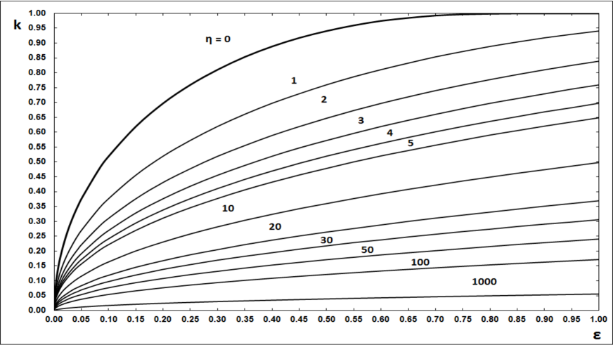
Figure 1: Dependence of characteristic number $k$ on degree of absorption $\varepsilon$ at $\overline{b}_{1}=1$. The numbers denote the value of parameter $\eta$.

In Table 2 we demonstrate how the presence of the second component, i.e. the free non-absorbing electrons, affects the value of characteristic number. Physically clear that for $\eta>1$ the mean effective absorption diminishes, i.e. the value $k$ also diminishes. Tables 1, 2 and Fig.1 demonstrate this feature for all range of parameter $\eta$ . The large values $\eta$ corresponds to small $k$ (see Fig.1). Recall, that Fig.1 corresponds to $\overline{b}_{1}=1$. Clearly, the small characteristic number does not give very sharp angular dependence of the radiation intensity $J(\mu)$. The case $\eta\to\infty$ corresponds to the free electron atmosphere.

The value $J(\mu=1)=3.06$ for $k=0$ and spherical polarizability ($\overline{b}_{1}=1$) for non - absorbing particles is Chandrasekhar’s (1960) case. This case gives the polarization $p(\mu=0)=11.71\%$. In Table 3 we present also the Milne problem solutions for needle like particles ($\overline{b}_{1}=0.4$) and plate like ones ($\overline{b}_{1}=0.7$) . The needle like particles give $J(\mu=1)=2.96$ and corresponding maximum polarization $p(\mu=0)=3.80\%$ . For plate like grains we have $J(\mu=1)=3.00$ and $p(\mu=0)=7.26\%$.

For $\varepsilon=0.1$ and $\eta=0$ the corresponding results are given in Table 4. It is seen that the nonzero absorption increases the polarization values for all forms of dust grains. The case $\eta\neq 0$ diminishes the polarization degree, as it is seen from Table 5.

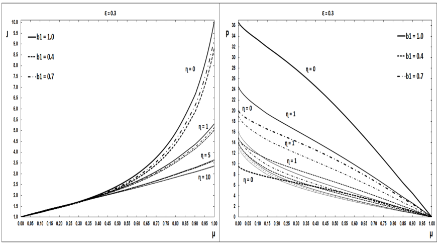
Figure 5: The angular distribution $J(\mu)$ and polarization degree $p(\mu)$ in % for different forms of dust grains ($\overline{b}_{1}=1,0.70.4$ , describing by continuous, chain-dotted and short-dotted lines, respectively ) and the values $\eta=0,1,5,10$. The thicknesses of curves diminish corresponding to values $\eta=0,1,5,10$. The degree of absorption $\varepsilon=0.3$.

We see that the presence of absorption ($\varepsilon=0.1$) considerably increases the polarization values $p(\mu=0)=20.35\%,5.48\%,11.18\%$, for $\overline{b}_{1}=1,04,0.7$, respectively. The angular dependence also increase, $J(\mu=1)=4.39,4.02,$ $4.15$, respectively. For $\varepsilon=0.1$ and $\eta=1$ (see Fig. 5) the results are: $p(\mu=0)=16.07\%$,

$8.45\%,12.35\%$ and $J(\mu=1)=3.66,3.46,3.58$, respectively.

It is seen that anisotropy of particles considerably changes the polarization of emerging radiation. The angular distribution $J(\mu)$ for all cases is near for $\overline{b}_{1}=1$ case. Note that the polarization from needle like particles is smaller than that from plate like ones.

The limit case of $\varepsilon=1$ (pure absorbing dust grains) for $\eta=1,5$ and 10 is presented in Table 6. Note that for $\eta\to\infty$ the angular distribution and degree of polarization tend to values in Table 3 (two first columns).

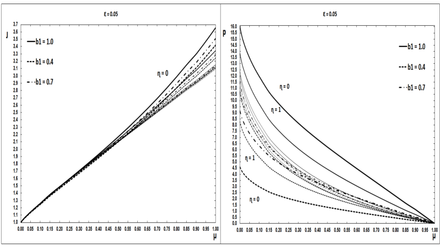
Figure 2: The angular distribution $J(\mu)$ and polarization degree $p(\mu)$ in % for different forms of dust grains ($\overline{b}_{1}=1,0.7,0.4$ , describing by continuous, chain-dotted and short-dotted lines, respectively ) and the values $\eta=0,1,5,10$. The thicknesses of curves diminish corresponding to values $\eta=0,1,5,10$ .The degree of absorption $\varepsilon=0.05$.

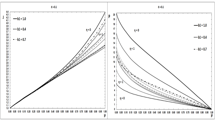
Figure 3: The angular distribution $J(\mu)$ and polarization degree $p(\mu)$ in % for different forms of dust grains ($\overline{b}_{1}=1,0.7,0.4$, describing by continuous, chain-dotted and short-dotted lines, respectively ) and the values $\eta=0,1,5,10$. The thicknesses of curves diminish corresponding to values $\eta=0,1,5,10$. The degree of absorption $\varepsilon=0.1$.

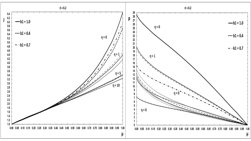
Figure 4: The angular distribution $J(\mu)$ and polarization degree $p(\mu)$ in % for different forms of dust grains ($\overline{b}_{1}=1,0.7,0.4$, describing by continuous, chain-dotted and short-dotted lines, respectively ) and the values $\eta=0,1,5,10$. The thicknesses of curves diminish corresponding to values $\eta=0,1,5,10$. The degree of absorption $\varepsilon=0.2$.

Figs. 2-5 present the values of angular distribution of radiation $J(\mu)$ and polarization degrees $p(\mu)$ in % for parameters $\eta=0,1,5,10$, $\varepsilon=0.05,0.1,0.2,0.3$ and $\overline{b}_{1}=1,0.4,0.7$. It is seen that cases $\eta=5$ and $10$ are close to free electron scattering.

Finally, we give short description of results in Figs. 2-5. First, the cases of spherical grains ($\overline{b}_{1}=1$ presented by the continuous curves) have the greater $J(\mu)$ and $p(\mu)$ than those for the anisotropic grains ($\overline{b}=0.7,0.4$, the chain-dotted line and short-dotted lines, respectively). The increase of the parameter $\eta$ diminishes the polarization curves for $\overline{b}_{1}=1$ case. In contrast, polarization curves for $\overline{b}_{1}=0.4$ increase with the increasing of $\eta$. In the limit of great $\eta$ all curves tends to the electron scattering case with effective absorption $\varepsilon_{eff}=1/(1+\eta)$.

Table 1: The characteristic number $k$ for $\eta=0$ and $\overline{b}_{1}=1,0.4,0.7$ corresponding to spherical, needle like and plate like particles, respectively

$\varepsilon$	$\overline{b}_{1}=1$	$\overline{b}_{1}=0.4$	$\overline{b}_{1}=0.7$	$k_{appr}$
0	0	0	0	0
0.001	0.054743	0.054749	0.054747	0.05477
0.01	0.172285	0.172473	0.172417	0.17350
0.05	0.377166	0.379075	0.378489	0.38730
0.1	0.519583	0.524331	0.522813	0.54772
0.2	0.697604	0.707702	0.704204	0.77460
0.3	0.811199	0.824504	0.819545	-
0.4	0.888707	0.902445	0.896992	-
0.5	0.941298	0.952885	0.948054	-
0.6	0.974750	0.982379	0.979104	-
0.7	0.992822	0.996093	0.994698	-
0.8	0.999292	0.999774	0.999588	-
0.9	0.999999	0.999999	0.999999	-
1	1	0.999999	0.999999	-

Table 2: The characteristic number $k$ for $\eta=5$ and $\overline{b}_{1}=1,0.4,0.7$ corresponding to spherical, needle like and plate like particles, respectively

$\varepsilon$	$\overline{b}_{1}=1.$	$\overline{b}_{1}=0.4$	$\overline{b}_{1}=0.7$	$k_{appr}$
0	0	0	0	0
0.001	0.022359	0.022359	0.022359	0.02236
0.01	0.070648	0.070652	0.070650	0.07071
0.05	0.157413	0.157458	0.157438	0.15811
0.1	0.221632	0.221750	0.221697	0.22361
0.2	0.310678	0.310969	0.310836	0.31623
0.3	0.377166	0.377625	0.377412	0.38730
0.4	0.431710	0.432302	0.432024	-
0.5	0.478465	0.479138	0.478818	-
0.6	0.519582	0.520273	0.519941	-
0.7	0.549302	0.556990	0.556682	-
0.8	0.589629	0.590134	0.589887	-
0.9	0.620005	0.620297	0.620152	-
1	0.647915	0.647915	0.647915	-

Table 3: The angular distribution $J(\mu)$ and degree of polarization $p(\mu)=-Q(\mu)/I(\mu)$ in % for $\varepsilon=0$ and $\eta=0$ for different forms of particles ($\overline{b}_{1}=1,0.4,0.7$). Here all the characteristic numbers $k$ are equal to zero.

$\mu$	$J_{1}$	$p_{1}$	$J_{0.4}$	$p_{0.4}$	$J_{0.7}$	$p_{0.7}$
0	1	11.713	1	3.80	1	7.26
0.01	1.036	10.878	1.035	3.44	1.036	6.66
0.02	1.066	10.295	1.064	3.20	1.065	6.25
0.03	1.094	9.805	1.091	3.02	1.093	5.91
0.04	1.120	9.374	1.116	2.85	1.118	5.61
0.05	1.146	8.986	1.140	2.71	1.143	5.35
0.06	1.170	8.631	1.164	2.57	1.167	5.11
0.07	1.194	8.304	1.187	2.46	1.191	4.89
0.08	1.218	8.000	1.210	2.35	1.214	4.69
0.09	1.241	7.716	1.232	2.25	1.237	4.51
0.10	1.264	7.449	1.254	2.16	1.259	4.34
0.15	1.375	6.312	1.371	1.74	1.378	4.55
0.20	1.483	5.410	1.472	1.46	1.482	3.01
0.25	1.587	4.667	1.571	1.24	1.584	2.57
0.30	1.690	4.041	1.669	1.06	1.683	2.20
0.35	1.791	3.502	1.765	0.90	1.782	1.89
0.40	1.892	3.033	1.860	0.77	1.879	1.63
0.45	1.991	2.619	1.954	0.66	1.975	1.40
0.50	2.091	2.252	2.048	0.56	2.071	1.19
0.55	2.189	1.923	2.141	0.48	2.167	1.01
0.60	2.287	1.627	2.234	0.40	2.262	0.85
0.65	2.385	1.358	2.326	0.33	2.356	0.71
0.70	2.483	1.113	2.418	0.27	2.450	0.57
0.75	2.580	0.888	2.510	0.21	2.544	0.46
0.80	2.677	0.682	2.601	0.16	2.638	0.35
0.85	2.774	0.492	2.692	0.11	2.731	0.25
0.90	2.870	0.316	2.774	0.08	2.815	0.16
0.91	2.890	0.282	2.793	0.07	2.834	0.15
0.92	2.909	0.249	2.811	0.06	2.853	0.13
0.93	2.928	0.216	2.829	0.05	2.871	0.11
0.94	2.947	0.184	2.847	0.04	2.890	0.10
0.95	2.967	0.152	2.865	0.04	2.909	0.08
0.96	2.986	0.121	2.883	0.03	2.927	0.06
0.97	3.005	0.090	2.902	0.02	2.946	0.05
0.98	3.015	0.060	2.920	0.01	2.964	0.03
0.99	3.044	0.030	2.938	0.01	2.983	0.02
1	3.063	0	2.956	0	3.002	0

Table 4: The angular distribution $J(\mu)$ and degree of polarization $p(\mu)=-Q(\mu)/I(\mu)$ in % for $\varepsilon=0.1$ and $\eta=0$ for different forms of particles ($\overline{b}_{1}=1(k=0.519582),0.4(k=0.524331),0.7(k=0.522813)$)

. $\mu$ $J_{1}$ $p_{1}$ $J_{0.4}$ $p_{0.4}$ $J_{0.7}$ $p_{0.7}$ 0 1 20.348 1 5.48 1 11.19 0.01 1.033 19.606 1.033 5.14 1.033 10.62 0.02 1.061 19.081 1.060 4.91 1.061 10.23 0.03 1.087 18.636 1.085 4.73 1.086 9.91 0.04 1.111 18.239 1.109 4.57 1.111 9.62 0.05 1.135 17.879 1.133 4.42 1.135 9.37 0.06 1.159 17.545 1.155 4.29 1.158 9.14 0.07 1.182 17.233 1.178 4.18 1.181 8.92 0.08 1.205 16.939 1.200 4.07 1.203 8.73 0.09 1.227 16.660 1.222 3.97 1.225 8.54 0.10 1.249 16.395 1.243 3.87 1.247 8.36 0.15 1.371 15.099 1.360 3.44 1.366 7.54 0.20 1.481 14.080 1.465 3.12 1.474 6.93 0.25 1.594 13.146 1.571 2.86 1.583 6.39 0.30 1.710 12.264 1.680 2.62 1.694 5.91 0.35 1.831 11.413 1.792 2.41 1.809 5.46 0.40 1.957 10.576 1.908 2.21 1.929 5.02 0.45 2.090 9.746 2.029 2.02 2.055 4.61 0.50 2.231 8.914 2.156 1.83 2.187 4.20 0.55 2.381 8.075 2.290 1.65 2.326 3.79 0.60 2.541 7.226 2.431 1.47 2.475 3.39 0.65 2.712 6.365 2.582 1.29 2.633 2.98 0.70 2.897 5.489 2.744 1.11 2.802 2.57 0.75 3.098 4.598 2.917 0.93 2.985 2.15 0.80 3.316 3.691 3.105 0.74 3.183 1.73 0.85 3.554 2.767 3.308 0.56 3.398 1.30 0.90 3.789 1.923 3.507 0.39 3.609 0.90 0.91 3.843 1.733 3.553 0.35 3.659 0.81 0.92 3.899 1.543 3.601 0.31 3.709 0.72 0.93 3.957 1.352 3.649 0.27 3.760 0.64 0.94 4.015 1.161 3.698 0.24 3.812 0.55 0.95 4.075 0.969 3.748 0.20 3.865 0.46 0.96 4.135 0.776 3.799 0.16 3.920 0.36 0.97 4.197 0.583 3.852 0.12 3.975 0.27 0.98 4.261 0.389 3.905 0.08 4.032 0.18 0.99 4.326 0.195 3.959 0.04 4.090 0.09 1 4.392 0 4.015 0 4.149 0

Table 5: The angular distribution $J(\mu)$ and degree of polarization $p(\mu)=-Q(\mu)/I(\mu)$ in % for $\varepsilon=0.1$ and $\eta=1$ for different forms of particles ($\overline{b}_{1}=1(k=0.377166),0.4(k=0.378446),0.7(k=0.377953)$)

. $\mu$ $J_{1}$ $p_{1}$ $J_{0.4}$ $p_{0.4}$ $J_{0.7}$ $p_{0.7}$ 0 1 16.073 1 8.45 1 12.35 0.01 1.035 15.283 1.035 7.86 1.035 11.65 0.02 1.064 14.729 1.063 7.46 1.064 11.17 0.03 1.904 14.261 1.089 7.14 1.090 10.76 0.04 1.116 13.846 1.115 6.85 1.116 10.40 0.05 1.141 13.472 1.139 6.60 1.140 10.08 0.06 1.165 13.127 1.162 6.37 1.164 9.79 0.07 1.188 12.807 1.185 6.16 1.187 9.52 0.08 1.211 12.508 1.208 5.96 1.210 9.27 0.09 1.234 12.227 1.230 5.78 1.233 9.03 0.10 1.257 11.960 1.253 5.62 1.255 8.81 0.15 1.379 10.694 1.371 4.84 1.376 7.78 0.20 1.487 9.744 1.476 4.30 1.483 7.02 0.25 1.596 8.914 1.580 3.84 1.590 6.37 0.30 1.706 8.168 1.685 3.45 1.698 5.80 0.35 1.817 7.479 1.791 3.11 1.807 5.28 0.40 1.931 6.833 1.898 2.80 1.918 4.80 0.45 2.048 6.216 2.007 2.52 2.032 4.35 0.50 2.168 5.622 2.119 2.25 2.148 3.92 0.55 2.291 5.042 2.234 2.00 2.268 3.50 0.60 2.420 4.472 2.352 1.76 2.392 3.10 0.65 2.553 3.908 2.473 1.53 2.521 2.70 0.70 2.691 3.347 2.599 1.30 2.654 2.31 0.75 2.836 2.784 2.730 1.08 2.793 1.92 0.80 2.988 2.226 2.866 0.86 2.938 1.53 0.85 3.146 1.662 3.008 0.64 3.090 1.14 0.90 3.297 1.151 3.141 0.44 3.233 0.79 0.91 3.331 1.037 3.171 0.40 3.265 0.71 0.92 3.366 0.922 3.202 0.35 3.298 0.63 0.93 3.401 0.808 3.233 0.31 3.331 0.55 0.94 3.436 0.693 3.264 0.26 3.365 0.48 0.95 3.472 0.578 3.295 0.22 3.399 0.40 0.96 3.508 0.463 3.327 0.18 3.434 0.32 0.97 3.545 0.348 3.359 0.13 3.468 0.24 0.98 3.582 0.232 3.392 0.09 3.503 0.16 0.99 3.619 0.116 3.425 0.04 3.539 0.08 1 3.657 0 3.458 0 3.575 0

Table 6: The angular distribution $J(\mu)$ and degree of polarization $p(\mu)=-Q(\mu)/I(\mu)$ in % for limit case of pure absorbing grains $\varepsilon=1$. The columns correspond to $\eta=1(k=0.94129807),5(k=0.64791542),10(k=0.49776253)$

. $\mu$ $J_{1}$ $p_{1}$ $J_{5}$ $p_{5}$ $J_{10}$ $p_{10}$ 0 1 52.55 1 25.91 1 19.58 0.01 1.022 52.19 1.031 25.23 1.034 18.83 0.02 1.042 51.91 1.058 24.75 1.062 18.30 0.03 1.060 51.65 1.082 24.33 1.087 17.85 0.04 1.079 51.40 1.106 23.96 1.112 17.45 0.05 1.097 51.16 1.129 23.62 1.136 17.09 0.06 1.116 50.91 1.151 23.30 1.160 16.75 0.07 1.134 50.65 1.174 23.00 1.183 16.43 0.08 1.153 50.40 1.196 22.72 1.206 16.14 0.09 1.172 50.14 1.218 22.44 1.228 15.86 0.10 1.191 49.87 1.239 22.18 1.251 15.59 0.15 1.302 48.25 1.360 20.84 1.372 14.30 0.20 1.414 46.54 1.472 19.72 1.482 13.30 0.25 1.541 44.61 1.589 18.65 1.594 12.38 0.30 1.687 42.45 1.713 17.58 1.710 11.53 0.35 1.855 40.08 1.845 16.50 1.829 10.70 0.40 2.051 37.51 1.987 15.40 1.953 9.90 0.45 2.283 34.78 2.141 14.28 2.083 9.11 0.50 2.561 31.89 2.309 13.12 2.220 8.32 0.55 2.898 28.88 2.494 11.93 2.365 7.53 0.60 3.315 25.77 2.698 10.71 2.319 6.73 0.65 3.840 22.57 2.925 9.46 2.683 5.93 0.70 4.520 19.32 3.180 8.17 2.859 5.11 0.75 5.430 16.04 3.468 6.85 3.049 4.28 0.80 6.706 12.74 3.797 5.50 3.254 3.43 0.85 8.610 9.44 4.174 4.12 3.477 2.57 0.90 11.342 6.48 4.565 2.86 3.694 1.79 0.91 12.171 5.82 4.660 2.58 3.744 1.61 0.92 13.116 5.17 4.757 2.30 3.796 1.43 0.93 14.206 4.52 4.858 2.01 3.849 1.26 0.94 15.475 3.87 4.963 1.73 3.902 1.08 0.95 16.970 3.22 5.071 1.44 3.957 0.90 0.96 18.759 2.57 5.183 1.15 4.012 0.72 0.97 20.937 1.93 5.299 0.87 4.069 0.54 0.98 23.645 1.28 5.419 0.58 4.127 0.36 0.99 27.103 0.64 5.543 0.29 4.186 0.18 1 3.657 0 3.458 0 3.575 0

5 Conclusion

We consider the generalized Milne problem in two components non-conservative atmosphere - free electrons and small absorbing anisotropic grains. The radiative transfer equation in such atmosphere depends on two parameters $W$ and $(a+b)$, which depend on three physical parameters. Parameter $\eta$ is the ratio of the Thomson optical length to that due to small grains. The value $\overline{b}_{1}$ characterizes radiation scattered in accordance with Rayleigh phase matrix and the parameter $\overline{b}_{2}$ (depolarization parameter) describes the isotropic scattering. These values obey the relation $\overline{b}_{1}+3\overline{b}_{2}=1$. The third parameter $\varepsilon=\sigma^{(a)}_{grain}/\sigma^{(t)}_{grain}$ is the degree of radiation absorption by dust grains. We use the matrix resolvent function $\hat{R}(\tau,\tau^{\prime})$ approach (see Silant’ev et al. 2015). This matrix is connected with two auxiliary matrices, depending on one variable - $R(\tau,0)$ and $R(0,\tau^{\prime})$. The Laplace transform of the matrix $R(\tau,0)$ with the parameter $1/\mu$ is the matrix $\hat{H}(\mu)$ function, which obeys the nonlinear matrix equation similar to known system of equations for Chandrasekhar’s scalar $H$- functions. This matrix obeys also the linear integral equation with singular kernel. This linear equation was derived in algebraic manner from the of nonlinear equation for matrix $\hat{H}(\mu)$ . Our calculations demonstrate that even small number of dust grains in an atmosphere changes significantly the polarization of outgoing radiation as compared with known Chandrasekhar’s value of polarization for free electron atmosphere.

Acknowledgements. This research was supported by the Program of Prezidium of Russian Academy of Sciences N 17, by the Program of the Department of Physical Sciences of Russian Academy of Sciences N 2 and the president program ” the leading scientific schools” N 7241.

The authors are very grateful to Dr. H. Frisch for a number of useful remarks, especially for new factorization (9).

References

- [1] Abhyankar, K. D., Fymat, A. L. Astrophys. J. Suppl. Ser. 23, 35 (1971)
- [2] Chandrasekhar, S.: Radiative transfer. Dover, New York (1960)
- [3] Dolginov, A. Z., Gnedin, Yu. N., Silant’ev, N. A. : Propagation and Polarization of Radiation in Cosmic Media. Gordon & Breach Publ., Amsterdam (1995)
- [4] Frisch, H. private communication (2017)
- [5] Frölich, H.: Theory of dielectrics. Clarendon Press, Oxford (1958)
- [6] Greenberg, J. M.: Interstellar grains. In Stars and Stellar systems. Vol.VII, Ch.6, The University of Chicago Press, Chicago (1968)
- [7] Hulst, H. G. van de: Multiple Light Scattering. Academic Press, New York (1980)
- [8] Lenoble J. J. Quant. Spectrosc. Radiat. Transf. 10, 533 (1970)
- [9] Schnatz, T. W., Siewert, C. E. , MNRAS 152, 491 (1971)
- [10] Silant’ev, N. A., SvA, 24, 341 (1980)
- [11] Silant’ev, N. A., Astron. report, 51, 67 (2007)
- [12] Silant’ev, N. A., Alekseeva, G. A., Novikov, V. V., Astrophys. Space Sci. 357, 53 (2015)
- [13] Sobolev, V. V. : Course in theoretical astrophysics. NASA Technical Translation F-531, Washington (1969)