Bayesian Estimation of Kendall’s $\tau$ Using a Latent Normal Approach

Abstract

The rank-based association between two variables can be modeled by introducing a latent normal level to ordinal data. We demonstrate how this approach yields Bayesian inference for Kendall’s $\tau$, improving on a recent Bayesian solution based on its asymptotic properties.

1 A Bayesian Framework for Kendall’s $\tau$

Kendall’s $\tau$ is a popular rank-based correlation coefficient. Compared to Pearson’s $\rho$, Kendall’s $\tau$ is robust to outliers, invariant under monotonic transformations, and has an intuitive interpretation (Kendall and Gibbons, 1990). Let $X=(x_{1},...,x_{n})$ and $Y=(y_{1},...,y_{n})$ be two data vectors each containing ranked measurements of the same $n$ units. For instance, $x$ could be the rank ordered scores on a math exam and $y$ the rank ordered scores on a geography exam, for $n$ test-takers. A concordant pair is then defined as a pair of subjects $(i,j)$ where subject $i$ has a higher score on $x$ and $y$ compared to subject $j$, whereas a discordant pair is defined as one where $i$ scores higher on $y$, but $j$ scores higher on $x$, or the other way around. Kendall’s $\tau$ is defined as the difference between the number of concordant and discordant pairs, expressed as proportion of the total number of pairs:

$$\tau=\frac{\sum_{1\leq i<j\leq n}^{n}Q((x_{i},y_{i}),(x_{j},y_{j}))}{n(n-1)/2},$$ (1)

where the denominator is the total number of pairs and $Q$ is the concordance indicator function, which is defined by:

$$Q((x_{i},y_{i})(x_{j},y_{j}))=\begin{cases}-1&\text{if }(x_{i}-x_{j})(y_{i}-y_{j})<0\\ +1&\text{if }(x_{i}-x_{j})(y_{i}-y_{j})>0\\ \end{cases}.$$ (2)

The function returns $-1$ if a pair is discordant, and returns +1 if a pair is concordant. However, due to the nonparametric nature of Kendall’s $\tau$ and the lack of a likelihood function for the data, Bayesian inference is not trivial.

An innovative method for overcoming this problem was proposed by Johnson (2005), and involves the modeling of the test statistic itself, rather than the data. This method has been applied to Kendall’s $\tau$ by Yuan and Johnson (2008), and was recently developed by van Doorn, Ly, Marsman, and Wagenmakers (2018). The inferential framework that follows from this work uses the limiting normal distribution of the test statistic $T^{*}$ (Hotelling and Pabst, 1936; Noether, 1955), where

$$T^{*}=\tau\sqrt{\frac{9n(n-1)}{4n+10}}.$$ (3)

Under $\mathcal{H}_{0}$, this limiting normal distribution is the standard normal, whereas under $\mathcal{H}_{1}$, this distribution is specified with a non-centrality parameter $\Delta$ for the mean, and a sampling variance of 1.

However, the method —henceforth the original asymptotic method— might fall short on two counts. Firstly, the asymptotic assumptions only hold for sufficiently large $n$ (i.e., $n$ $\geq$ 20, see van Doorn et al., 2018). Secondly, the variance of the sampling distribution of the test statistic depends on the population value of Kendall’s $\tau$. For $\tau=0$, the sampling variance equals 1, but as $\mid\tau\mid\rightarrow 1$, the variance decreases to $0$ (Kendall and Gibbons, 1990; Hotelling and Pabst, 1936).

In the current article, we will explore two corrections that aim to improve Bayesian inference for Kendall’s $\tau$:

1. Within the asymptotic framework, the observed value of Kendall’s $\tau$ can be used to set its sampling variance. We label this the enhanced asymptotic method.

2. Within a Bayesian latent normal framework, a latent level correlation is obtained and transformed to Kendall’s $\tau$. We label this the latent normal method.

2 Correction Using The Sample $\tau$

A first correction to consider is to use the sample value of Kendall’s $\tau$, denoted $\tau_{obs}$, to estimate the sampling variance of $T^{*}$, denoted $\sigma^{2}_{T^{*}}$. A convenient expression for the upper bound of $\sigma^{2}_{T^{*}}$ in terms of $\tau$ is given in Kendall and Gibbons (1990):

$$\sigma^{2}_{T^{*}}\leq\frac{2.5n(1-\tau^{2})}{2n+5}.$$ (4)

Using $\tau_{obs}$ as an estimate of $\tau$ provides a somewhat crude approximation to the sampling distribution of $T^{*}$. However, compared to using $\sigma^{2}_{T^{*}}=1$ as in the original asymptotic method, working with the upper bound will result in a more narrow posterior for cases where $\tau\neq 0$. However, the enhanced asymptotic method still suffers from the use of asymptotic assumptions about the sampling distribution and variance of the test statistic.

3 Correction Using The Latent Normal Approach

3.1 Latent Normal Models

Several latent variable models quantify the association between two ordinal variables. These methods often introduce a latent bivariate normal distribution to the ordinal variables, where the association between variables is modeled through a latent correlation (Pearson, 1900; Olssen, 1979; Pettitt, 1982; Albert, 1992; Alvo and Yu, 2014). The observed rank data $(x,y)$ can then be seen as the ordinal manifestations of the continuous latent variables $(z^{x},z^{y})$, which have a bivariate normal distribution. Figure 1 offers a graphical representation of such a model. Using this methodology, the nonparametric problem of ordinal analysis is transformed to a parametric data augmentation problem.

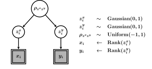
Figure 1: A graphical model of the latent normal method. Here, $x$ and $y$ are observed rank data. The latent level is denoted with $z^{x}$ and $z^{y}$, and $\rho_{z^{x}z^{y}}$ represents the latent correlation.

3.2 Posterior Distribution for the Latent Correlation

The joint posterior can be decomposed as follows:

$$P(z^{x},z^{y},\rho_{z^{x},z^{y}}\mid x,y)\propto P(x,y\mid z^{x},z^{y})\times P(z^{x},z^{y}\mid\rho_{z^{x},z^{y}})\times P(\rho_{z^{x},z^{y}}).$$ (5)

The second factor on the right-hand side is the bivariate normal distribution of the latent scores given the latent correlation:

$$\begin{pmatrix}z^{x}\\ z^{y}\end{pmatrix}\sim\mathcal{N}\begin{bmatrix}\begin{pmatrix}0\\ 0\end{pmatrix}\!\!,&\begin{pmatrix}1&\rho_{z^{x},z^{y}}\\ \rho_{z^{x},z^{y}}&1\\ \end{pmatrix}\end{bmatrix}.\\ \leavevmode\nobreak\ \newline$$ (6)

The factor $P(x,y\mid z^{x},z^{y})$ consists of a set of indicator functions that map the observed ranks to latent scores, such that the ordinal information is preserved. For the value $z^{x}_{i}$, this means that its range is truncated by the lower and upper thresholds that are respectively defined as:

$$a^{x}_{i}=\max\limits_{j:x_{j}<x_{i}}\left({z^{x}_{j}}\right)$$ (7)

$$b^{x}_{i}=\min\limits_{j:x_{j}>x_{i}}\left({z^{x}_{j}}\right).$$ (8)

The third factor is the prior distribution on the latent correlation. In the remainder of this article, the prior is specified by a uniform distribution on $(-1,1)$ (but see Berger and Sun 2008; Ly, Verhagen, and Wagenmakers 2016).

The general Bayesian framework for estimating the latent correlation involves data augmentation through a Gibbs sampling algorithm (Geman and Geman, 1984), combined with a random walk Metropolis-Hastings sampling algorithm. At sampling time point $s$:

1. For each value of $z^{x}_{i}$, sample from a truncated normal distribution, where the lower threshold is $a^{x}_{i}$ given in (7) and the upper threshold is $b^{x}_{i}$ given in (8):

   $$(z_{i}^{x}\mid z_{i^{\prime}}^{x},z_{i}^{y},\rho_{z^{x},z^{y}})\sim N\left(z_{i}^{y}\rho_{z^{x},z^{y}},\sqrt{1-\rho^{2}_{z^{x},z^{y}}}\right)\delta_{a^{x}_{i},b^{x}_{i}}$$

2. For each value of $z^{y}_{i}$, the sampling procedure is analogous to step 1.

3. Sample a new proposal for $\rho_{z^{x},z^{y}}$, denoted $\rho^{*}_{z^{x},z^{y}}$, from the asymptotic normal approximation to the sampling distribution of Fisher’s z-transform of $\rho$ (Fisher, 1915):

   $$\tanh^{-1}(\rho^{*}_{z^{x},z^{y}})\sim N\left(\tanh^{-1}\left(\rho^{s-1}_{z^{x},z^{y}}\right),\frac{1}{\sqrt{(n-3)}}\right).$$

   The acceptance rate $\alpha$ is determined by the likelihood ratio of $(z^{x},z^{y}\mid\rho^{*}_{z^{x},z^{y}})$ and $(z^{x},z^{y}\mid\rho^{s-1}_{z^{x},z^{y}})$, where each likelihood is determined by the bivariate normal distribution in (6):

   $$\alpha=\min\left(1,\frac{P(z^{x},z^{y}\mid\rho^{*}_{z^{x},z^{y}})}{P(z^{x},z^{y}\mid\rho^{s-1}_{z^{x},z^{y}})}\right).$$

Repeating the algorithm a sufficient number of times yields samples from the posterior distributions of $z^{x},z^{y},$ and $\rho_{z^{x},z^{y}}$.

3.3 Relation to Kendall’s $\tau$

With the posterior distribution for the latent $\rho_{z^{x},z^{y}}$ in hand, the transition to the posterior distribution for Kendall’s $\tau$ can be made using Greiner’s relation (Greiner, 1909; Kruskal, 1958). This relation, defined as

$$\tau=G(\rho)=\frac{2}{\pi}\sin^{-1}(\rho)$$ (9)

enables the transformation of Pearson’s $\rho$ to Kendall’s $\tau$ when the data follow a bivariate normal distribution.

Using Greiner’s relation, the posterior distribution of Kendall’s $\tau$ can be rewritten as follows:

$$P(\tau\mid x,y)\approx P(G(\rho)\mid x,y)=\int\int P(G(\rho)\mid z^{x},z^{y})P(z^{x},z^{y}\mid x,y)dz^{x}dz^{y}.$$

Introducing the latent normal level to the observed variables enables the link between Pearson’s $\rho$ and Kendall’s $\tau$, and turns posterior inference for Kendall’s $\tau$ into a parametric data augmentation problem that can be solved with the above MCMC-methods. Thus, Greiner’s relation can be applied to the posterior samples of $\rho_{z^{x},z^{y}}$ to yield posterior samples of $\tau$.

Furthermore, the application of Greiner’s relation in this manner implicitly alters the prior from a uniform distribution on the latent correlation to the following distribution on Kendall’s $\tau$:

$$p(\tau)=\frac{\pi}{4}\cos\left(\frac{\pi\tau}{2}\right)\text{, for }\tau\in(-1\text{, }1).$$ (10)

4 Results: Simulation Study

The performance of the original asymptotic method, the enhanced asymptotic method, and the latent normal method was assessed with a simulation study. For four values of $\tau$ (0, 0.2, 0.4, 0.7) and three values of $n$ (10, 20, 50), $10{,}000$ data sets were generated under four copula models: Clayton, Gumbel, Frank, and Gaussian (Sklar, 1959; Nelsen, 2006; Genest and Favre, 2007; Colonius, 2016). Using Sklar’s theorem, copula models decompose a joint distribution into univariate marginal distributions and a dependence structure (i.e., the copula). The aforementioned copulas are governed by Kendall’s $\tau$, so the performance of each method can be assessed through a parameter recovery simulation study. Furthermore, the univariate marginal distributions can be transformed to any other distribution using the cumulative distribution function and its inverse. Because these functions are monotonic, this does not affect the copula or ordinal information in the synthetic data and therefore vastly increases the scope of the simulation study.

For each data set, a posterior distribution was obtained using the three methods and the population value of $\tau$ was estimated using the posterior median. Per combination of $n$ and $\tau$, this resulted in $10,000$ posterior distributions. For an overall view of each method’s performance, Figure 2 shows the quantile averaged posterior distributions, along with a vertical line indicating the population value of $\tau$. The data in Figure 2 were generated using the Clayton copula; other copula models yielded highly similar results. The quantile averaged posteriors indicate no difference between the inferential methods under $\mathcal{H}_{0}$, which corroborates the assumption of $\sigma^{2}_{T^{*}}=1$ when $\tau=0$. However, the difference in methods becomes pronounced in the scenario where $n=10$ and $\tau=0.7$. Both asymptotic approaches show a degree of underestimation, and yield a relatively broad posterior distribution. In the panels where $\tau\neq 0$, the misspecification of the sampling variance also becomes clear, as it is overestimated and results in a wider posterior distribution compared to the latent normal method. Although the assumption of latent normality is the price to pay for the Bayesian latent normal methodology, the simulation results indicate robustness of the method to various violations of this assumption.

5 Discussion

This article has outlined two methods of improving the Bayesian inferential framework in cases where $n$ is low and/or $\tau$ is high. Although an extension of the asymptotic framework performs somewhat better than the original asymptotic framework in van Doorn et al. (2018), both are outperformed by the latent normal approach. Under $\mathcal{H}_{0}$, the methods do not differ from each other, underscoring the validity of the general framework.

The outlined methods are useful for both estimation and hypothesis testing. In the former case, the posterior distribution enables point estimation through the posterior median, or interval estimation through the credible interval. For hypothesis testing, the Savage-Dickey density ratio (Dickey and Lientz, 1970; Wagenmakers et al., 2010) can be used to obtain Bayes factors (Kass and Raftery, 1995). A concrete example is presented in the online appendix. Because the method uses only the ordinal information in the data, it retains the robust properties of Kendall’s $\tau$, such as invariance to monotone transformations, robustness to outliers or violations of normality, and ability to detect nonlinear monotone relations.

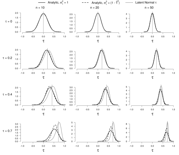
Figure 2: To illustrate the performance of the three methods, quantile averaged posterior distributions for several values of $\tau$ and $n$ are shown. Each column corresponds to a value of $n$, and each row corresponds to a value of $\tau$. The quantile averaged posterior distributions were obtained with 10,000 synthetic datasets per combination of $n$ and $\tau$. The vertical gray line indicates the population value of $\tau$.

6 Literature

References

- Albert (1992) Albert, J. H., 1992. Bayesian estimation of the polychoric correlation coefficient. Journal of statistical computation and simulation 44, 47–61.
- Alvo and Yu (2014) Alvo, M., Yu, P., 2014. Statistical Methods for Ranking Data. Frontiers in Probability and the Statistical Sciences. Springer New York, New York.
- Berger and Sun (2008) Berger, J. O., Sun, D., 2008. Objective priors for the bivariate normal model. The Annals of Statistics 36, 963–982.
- Colonius (2016) Colonius, H., 2016. An invitation to coupling and copulas: With applications to multisensory modeling. Journal of Mathematical Psychology 74, 2–10.
- Dickey and Lientz (1970) Dickey, J. M., Lientz, B. P., 1970. The weighted likelihood ratio, sharp hypotheses about chances, the order of a Markov chain. The Annals of Mathematical Statistics 41, 214–226.
- Fisher (1915) Fisher, R. A., 1915. Frequency distribution of the values of the correlation coefficient in samples from an indefinitely large population. Biometrika, 507–521.
- Geman and Geman (1984) Geman, S., Geman, D., 1984. Stochastic relaxation, Gibbs distributions and the Bayesian restoration of images. IEEE Transactions on Pattern Analysis and Machine Intelligence 6, 721–741.
- Genest and Favre (2007) Genest, C., Favre, A.-C., 2007. Everything you always wanted to know about copula modeling but were afraid to ask. Journal of Hydrologic Engineering 12, 347–368.
- Greiner (1909) Greiner, R., 1909. Über das Fehlersystem der Kollektivmasslehre. Zeitschift für Mathematik und Physik 57, 121–158.
- Hotelling and Pabst (1936) Hotelling, H., Pabst, M., 1936. Rank correlation and tests of significance involving no assumption of normality. Annals of Mathematical Statistics 7, 29–43.
- Johnson (2005) Johnson, V. E., 2005. Bayes factors based on test statistics. Journal of the Royal Statistical Society 67, 689–701.
- Kass and Raftery (1995) Kass, R. E., Raftery, A. E., 1995. Bayes factors. Journal of the American Statistical Association 90, 773–795.
- Kendall and Gibbons (1990) Kendall, M., Gibbons, J. D., 1990. Rank Correlation Methods. Oxford University Press, New York.
- Kruskal (1958) Kruskal, W., 1958. Ordinal measures of association. Journal of the American Statistical Association 53, 814–861.
- Ly et al. (2016) Ly, A., Verhagen, A. J., Wagenmakers, E.-J., 2016. Harold Jeffreys’s default Bayes factor hypothesis tests: Explanation, extension, and application in psychology. Journal of Mathematical Psychology 72, 19–32.
- Nelsen (2006) Nelsen, R., 2006. An Introduction to Copulas, 2nd Edition. Springer-Verlag New York.
- Noether (1955) Noether, G. E., 1955. On a theorem of Pitman. Annals of Mathematical Statistics 26, 64–68.
- Olssen (1979) Olssen, U., 1979. Maximum likelihood estimation of the polychoric correlation coefficient. Psychometrika 44, 443–460.
- Pearson (1900) Pearson, K., 1900. Mathematical contributions to the theory of evolution. vii. on the correlation of characters not quantitatively measurable. Philosophical Transactions of the Royal Society of London A: Mathematical, Physical and Engineering Sciences 195, 1–405.
- Pettitt (1982) Pettitt, A., 1982. Inference for the linear model using a likelihood based on ranks. Journal of the Royal Statistical Society. Series B 44, 234–243.
- Sklar (1959) Sklar, A., 1959. Fonctions de répartition à n dimensions et leurs marges. Publications de l’Institut de Statistique de L’Université de Paris 8, 229–231.
- van Doorn et al. (2018) van Doorn, J., Ly, A., Marsman, M., Wagenmakers, E.-J., 2018. Bayesian inference for Kendall’s rank correlation coefficient. The American Statistician, 1–6.
- Wagenmakers et al. (2010) Wagenmakers, E.-J., Lodewyckx, T., Kuriyal, H., Grasman, R., 2010. Bayesian hypothesis testing for psychologists: A tutorial on the Savage–Dickey method. Cognitive Psychology 60, 158–189.
- Yuan and Johnson (2008) Yuan, Y., Johnson, V. E., 2008. Bayesian hypothesis tests using nonparametric statistics. Statistica Sinica 18, 1185–1200.