Position-based coding and convex splitting for private communication over quantum channels

Abstract

The classical-input quantum-output (cq) wiretap channel is a communication model involving a classical sender $X$, a legitimate quantum receiver $B$, and a quantum eavesdropper $E$. The goal of a private communication protocol that uses such a channel is for the sender $X$ to transmit a message in such a way that the legitimate receiver $B$ can decode it reliably, while the eavesdropper $E$ learns essentially nothing about which message was transmitted. The $\varepsilon$-one-shot private capacity of a cq wiretap channel is equal to the maximum number of bits that can be transmitted over the channel, such that the privacy error is no larger than $\varepsilon\in(0,1)$. The present paper provides a lower bound on the $\varepsilon$-one-shot private classical capacity, by exploiting the recently developed techniques of Anshu, Devabathini, Jain, and Warsi, called position-based coding and convex splitting. The lower bound is equal to a difference of the hypothesis testing mutual information between $X$ and $B$ and the “alternate” smooth max-information between $X$ and $E$. The one-shot lower bound then leads to a non-trivial lower bound on the second-order coding rate for private classical communication over a memoryless cq wiretap channel.

1 Introduction

Among the many results of information theory, the ability to use the noise in a wiretap channel for the purpose of private communication stands out as one of the great conceptual insights [Wyn75]. A classical wiretap channel is modeled as a conditional probability distribution $p_{Y,Z|X}$, in which the sender Alice has access to the input $X$ of the channel, the legitimate receiver Bob has access to the output $Y$, and the eavesdropper Eve has access to the output $Z$. The goal of private communication is for Alice and Bob to use the wiretap channel in such a way that Alice communicates a message reliably to Bob, while at the same time, Eve should not be able to determine which message was transmitted. The author of [Wyn75] proved that the mutual information difference

$$\max_{p_{X}}\left[I(X;Y)-I(X;Z)\right]$$ (1.1)

is an achievable rate for private communication over the wiretap channel, when Alice and Bob are allowed to use it many independent times. Since then, the interest in the wiretap channel has not waned, and there have been many increasingly refined statements about achievable rates for private communication over wiretap channels [CK78, Hay06, Tan12, Hay13, YAG13, YSP16, TB16].

Many years after the contribution of [Wyn75], the protocol of quantum key distribution was developed as a proposal for private communication over a quantum channel [BB84]. Quantum information theory started becoming a field in its own right, during which many researchers revisited several of the known results of Shannon’s information theory under a quantum lens. This was not merely an academic exercise: doing so revealed that remarkable improvements in communication rates could be attained for physical channels of practical interest if quantum-mechanical strategies are exploited [GGL⁺04].

One important setting which was revisited is the wiretap channel, and in the quantum case, the simplest extension of the classical model is given by the classical-input quantum-output wiretap channel (abbreviated as cq wiretap channel) [Dev05, CWY04]. It is described as the following map:

$$x\rightarrow\rho_{BE}^{x},$$ (1.2)

where $x$ is a classical symbol that Alice can input to the channel and $\rho_{BE}^{x}$ is the joint output quantum state of Bob and Eve’s system, represented as a density operator acting on the tensor-product Hilbert space of Bob and Eve’s quantum systems. The goal of private communication over the cq wiretap channel is similar to that for the classical wiretap channel. However, in this case, Bob is allowed to perform a collective quantum measurement over all of his output quantum systems in order to determine Alice’s message, while at the same time, we would like for it be difficult for Eve to figure out anything about the transmitted message, even if she has access to a quantum computer memory that can store all of the quantum systems that she receives from the channel output. The authors of [Dev05, CWY04] independently proved that a quantum generalization of the formula in (1.1) is an achievable rate for private communication over a cq quantum wiretap channel, if Alice and Bob are allowed to use it many independent times. Namely, they proved that the following Holevo information difference is an achievable rate:

$$\max_{p_{X}}\left[I(X;B)-I(X;E)\right],$$ (1.3)

where the information quantities in the above formula are the Holevo information to Bob and Eve, respectively, and will be formally defined later in the present paper.

Since the developments of [Dev05, CWY04], there has been an increasing interest in the quantum information community to determine refined characterizations of communication tasks [TH13, Li14, TT15, DTW16, DHO16, DL15, BDL16, TBR16, WTB17], strongly motivated by the fact that it is experimentally difficult to control a large number of quantum systems, and in practice, one has access only to a finite number of quantum systems anyway. One such scenario of interest, as discussed above, is the quantum wiretap channel. Hitherto, the only work offering achievable one-shot rates for private communication over cq wiretap channels is [RR11]. However, that work did not consider bounding the second-order coding rate for private communication over the cq wiretap channel.

The main contribution of the present paper is a lower bound on the one-shot private capacity of a cq wiretap channel. Namely, I prove that

$$\log_{2}M_{\operatorname{priv}}^{\ast}(\varepsilon_{1}+\sqrt{\varepsilon_{2}})\geq I_{H}^{\varepsilon_{1}-\eta_{1}}(X;B)-\widetilde{I}_{\max}^{\sqrt{\varepsilon_{2}}-\eta_{2}}(E;X)-\log_{2}(4\varepsilon_{1}/\eta_{1}^{2})-2\log_{2}(1/\eta_{2}).$$ (1.4)

In the above, $\log_{2}M_{\operatorname{priv}}^{\ast}(\varepsilon_{1}+\sqrt{\varepsilon_{2}})$ represents the maximum number of bits that can be sent from Alice to Bob, using a cq wiretap channel once, such that the privacy error (to be defined formally later) does not exceed $\varepsilon_{1}+\sqrt{\varepsilon_{2}}\in(0,1)$, with $\varepsilon_{1},\varepsilon_{2}\in(0,1)$. The quantities on the right-hand side of the above inequality are particular one-shot generalizations of the Holevo information to Bob and Eve, which will be defined later. It is worthwhile to note that the one-shot information quantities in (1.4) can be computed using semi-definite programming, and the computational runtime is polynomial in the dimension of the channel. Thus, for channels of reasonable dimension, the quantities can be efficiently estimated numerically. The constants $\eta_{1}$ and $\eta_{2}$ are chosen so that $\eta_{1}\in(0,\varepsilon_{1})$ and $\eta_{2}\in(0,\sqrt{\varepsilon_{2}})$. By substituting an independent and identically distributed (i.i.d.) cq wiretap channel into the right-hand side of the above inequality, using second-order expansions for the one-shot Holevo informations [TH13, Li14], and picking $\eta_{1},\eta_{2}=1/\sqrt{n}$, we find the following lower bound on the second-order coding rate for private classical communication:

$$\log_{2}M_{\operatorname{priv}}^{\ast}(n,\varepsilon_{1}+\sqrt{\varepsilon_{2}})\geq n\left[I(X;B)-I(X;E)\right]\\ +\sqrt{nV(X;B)}\Phi^{-1}(\varepsilon_{1})+\sqrt{nV(X;E)}\Phi^{-1}(\varepsilon_{2})+O(\log n).$$ (1.5)

In the above, $\log_{2}M_{\operatorname{priv}}^{\ast}(n,\varepsilon_{1}+\sqrt{\varepsilon_{2}})$ represents the maximum number of bits that can be sent from Alice to Bob, using a cq wiretap channel $n$ times, such that the privacy error does not exceed $\varepsilon_{1}+\sqrt{\varepsilon_{2}}\in(0,1)$. The Holevo informations from (1.3) make an appearance in the first-order term (proportional to the number $n$ of channel uses) on the right-hand side above, while the second order term (proportional to $\sqrt{n}$) consists of the quantum channel dispersion quantities $V(X;B)$ and $V(X;E)$ [TT15], which will be defined later. They additionally feature the inverse $\Phi^{-1}$ of the cumulative Gaussian distribution function $\Phi$. Thus, the one-shot bound in (1.4) leads to a lower bound on the second-order coding rate, which is comparable to bounds that have appeared in the classical information theory literature [Tan12, YAG13, YSP16, TB16].

To prove the one-shot bound in (1.4), I use two recent and remarkable techniques: position-based coding [AJW17] and convex splitting [ADJ17]. The main idea of position-based coding [AJW17] is conceptually simple. To communicate a classical message from Alice to Bob, we allow them to share a quantum state $\rho_{RA}^{\otimes M}$ before communication begins, where $M$ is the number of messages, Bob possesses the $R$ systems, and Alice the $A$ systems. If Alice wishes to communicate message $m$, then she sends the $m$th $A$ system through the channel. The reduced state of Bob’s systems is then

$$\rho_{R_{1}}\otimes\cdots\otimes\rho_{R_{m-1}}\otimes\rho_{R_{m}B}\otimes\rho_{R_{m+1}}\otimes\cdots\otimes\rho_{R_{M}},$$ (1.6)

where $\rho_{R_{m}B}=\mathcal{N}_{A_{m}\rightarrow B}(\rho_{R_{m}A_{m}})$ and $\mathcal{N}_{A_{m}\rightarrow B}$ is the quantum channel. For all $m^{\prime}\neq m$, the reduced state for systems $R_{m^{\prime}}$ and $B$ is the product state $\rho_{R_{m^{\prime}}}\otimes\rho_{B}$. However, the reduced state of systems $R_{m}B$ is the (generally) correlated state $\rho_{R_{m}B}$. So if Bob has a binary measurement which can distinguish the joint state $\rho_{RB}$ from the product state $\rho_{R}\otimes\rho_{B}$ sufficiently well, he can base a decoding strategy off of this, and the scheme will be reliable as long as the number of bits $\log_{2}M$ to be communicated is chosen to be roughly equal to a one-shot mutual information known as hypothesis testing mutual information (cf., [WR12]). This is exactly what is used in position-based coding, and the authors of [AJW17] thus forged a transparent and intuitive link between quantum hypothesis testing and communication for the case of entanglement-assisted communication.

Convex splitting [ADJ17] is rather intuitive as well and can be thought of as dual to the coding scenario mentioned above. Suppose instead that Alice and Bob have a means of generating the state in (1.6), perhaps by the strategy mentioned above. But now suppose that Alice chooses the variable $m$ uniformly at random, so that the state, from the perspective of someone ignorant of the choice of $m$, is the following mixture:

$$\frac{1}{M}\sum_{m=1}^{M}\rho_{R_{1}}\otimes\cdots\otimes\rho_{R_{m-1}}\otimes\rho_{R_{m}B}\otimes\rho_{R_{m+1}}\otimes\cdots\otimes\rho_{R_{M}}.$$ (1.7)

The convex-split lemma guarantees that as long as $\log_{2}M$ is roughly equal to a one-shot mutual information known as the alternate smooth max-mutual information, then the state above is nearly indistinguishable from the product state $\rho_{R}^{\otimes M}\otimes\rho_{B}$.

Both position-based coding and convex splitting have been used recently and effectively to establish a variety of results in one-shot quantum information theory [AJW17, ADJ17]. In the present paper, I use the approaches in conjunction to construct codes for the cq wiretap channel. The main underlying idea follows the original approach of [Wyn75], by allowing for a message variable $m\in\{1,\ldots,M\}$ and a local key variable $k\in\{1,\ldots,K\}$ (local randomness), the latter of which is selected uniformly at random and used to confuse the eavesdropper Eve. Before communication begins, Alice, Bob, and Eve are allowed share to $MK$ copies of the common randomness state $\theta_{X_{A}X_{B}X_{E}}\equiv\sum_{x}p_{X}(x)|xxx\rangle\langle xxx|_{X_{A}X_{B}X_{E}}$. We can think of the $MK$ copies of $\theta_{X_{A}X_{B}X_{E}}$ as being partitioned into $M$ blocks, each of which contain $K$ copies of the state $\theta_{X_{A}X_{B}X_{E}}$. If Alice wishes to send message $m$, then she picks $k$ uniformly at random and sends the $(m,k)$ $X_{A}$ system through the cq wiretap channel in (1.2). As long as $\log_{2}MK$ is roughly equal to the hypothesis testing mutual information $I_{H}^{\varepsilon}(X;B)$, then Bob can use a position-based decoder to figure out both $m$ and $k$. As long as $\log_{2}K$ is roughly equal to the alternate smooth max-mutual information $\widetilde{I}_{\max}^{\varepsilon}(E;X)$, then the convex-split lemma guarantees that the overall state of Eve’s systems, regardless of which message $m$ was chosen, is nearly indistinguishable from the product state $\rho_{X_{E}}^{\otimes MK}\otimes\rho_{E}$. Thus, in such a scheme, Bob can figure out $m$ while Eve cannot figure out anything about $m$. This is the intuition behind the coding scheme and gives a sense of why $\log_{2}M=\log_{2}MK-\log_{2}K\approx I_{H}^{\varepsilon}(X;B)-\widetilde{I}_{\max}^{\varepsilon}(E;X)$ is an achievable number of bits that can be sent privately from Alice to Bob. The main purpose of the present paper is to develop the details of this argument and furthermore show how the scheme can be derandomized, so that the $MK$ copies of the common randomness state $\theta_{X_{A}X_{B}X_{E}}$ are in fact not necessary.

The rest of the paper proceeds as follows. In Section 2, I review some preliminary material, which includes several metrics for quantum states and pertinent information measures. Section 3 develops the position-based coding approach for classical-input quantum-output communication channels. Position-based coding was developed in [AJW17] to highlight a different approach to entanglement-assisted communication, but I show in Section 3 how the approach can be used for shared randomness-assisted communication; I also show therein how to derandomize codes in this case (i.e., the shared randomness is not actually necessary for classical communication over cq channels). Section 4 represents the main contribution of the present paper, which is a lower bound on the $\varepsilon$-one-shot private classical capacity of a cq wiretap channel. The last development in Section 4 is to show how the one-shot lower bound leads to a lower bound on the second-order coding rate for private classical communication over a memoryless cq wiretap channel. Therein, I also show how these lower bounds simplify for pure-state cq wiretap channels and when using binary phase-shift keying as a coding strategy for private communication over a pure-loss bosonic channel. Section 5 concludes with a summary and some open questions for future work.

2 Preliminaries

I use notation and concepts that are standard in quantum information theory and point the reader to [Wil16] for background. In the rest of this section, I review concepts that are less standard and set some notation that will be used later in the paper.

Trace distance, fidelity, and purified distance. Let $\mathcal{D}(\mathcal{H})$ denote the set of density operators acting on a Hilbert space $\mathcal{H}$, let $\mathcal{D}_{\leq}(\mathcal{H})$ denote the set of subnormalized density operators (with trace not exceeding one) acting on $\mathcal{H}$, and let $\mathcal{L}_{+}(\mathcal{H})$ denote the set of positive semi-definite operators acting on $\mathcal{H}$. The trace distance between two quantum states $\rho,\sigma\in\mathcal{D}(\mathcal{H})$ is equal to $\left\|\rho-\sigma\right\|_{1}$, where $\left\|C\right\|_{1}\equiv\operatorname{Tr}\{\sqrt{C^{{\dagger}}C}\}$ for any operator $C$. It has a direct operational interpretation in terms of the distinguishability of these states. That is, if $\rho$ or $\sigma$ are prepared with equal probability and the task is to distinguish them via some quantum measurement, then the optimal success probability in doing so is equal to $\left(1+\left\|\rho-\sigma\right\|_{1}/2\right)/2$. The fidelity is defined as $F(\rho,\sigma)\equiv\left\|\sqrt{\rho}\sqrt{\sigma}\right\|_{1}^{2}$ [Uhl76], and more generally we can use the same formula to define $F(P,Q)$ if $P,Q\in\mathcal{L}_{+}(\mathcal{H})$. Uhlmann’s theorem states that [Uhl76]

$$F(\rho_{A},\sigma_{A})=\max_{U}\left|\langle\phi^{\sigma}|_{RA}U_{R}\otimes I_{A}|\phi^{\rho}\rangle_{RA}\right|^{2},$$ (2.1)

where $|\phi^{\rho}\rangle_{RA}$ and $|\phi^{\sigma}\rangle_{RA}$ are fixed purifications of $\rho_{A}$ and $\sigma_{A}$, respectively, and the optimization is with respect to all unitaries $U_{R}$. The same statement holds more generally for $P,Q\in\mathcal{L}_{+}(\mathcal{H})$. The fidelity is invariant with respect to isometries and monotone non-decreasing with respect to channels. The sine distance or $C$-distance between two quantum states $\rho,\sigma\in\mathcal{D}(\mathcal{H})$ was defined as

$$C(\rho,\sigma)\equiv\sqrt{1-F(\rho,\sigma)}$$ (2.2)

and proven to be a metric in [Ras02, Ras03, GLN05, Ras06]. It was later [TCR09] (under the name “purified distance”) shown to be a metric on subnormalized states $\rho,\sigma\in\mathcal{D}_{\leq}(\mathcal{H})$ via the embedding

$$P(\rho,\sigma)\equiv C(\rho\oplus\left[1-\operatorname{Tr}\{\rho\}\right],\sigma\oplus\left[1-\operatorname{Tr}\{\sigma\}\right])\,.$$ (2.3)

The following inequality relates trace distance and purified distance:

$$\frac{1}{2}\left\|\rho-\sigma\right\|_{1}\leq P(\rho,\sigma).$$ (2.4)

Relative entropies and variances. The quantum relative entropy of two states $\omega$ and $\tau$ is defined as [Ume62]

$$D(\omega\|\tau)\equiv\operatorname{Tr}\{\omega[\log_{2}\omega-\log_{2}\tau]\}$$ (2.5)

whenever $\operatorname{supp}(\omega)\subseteq\operatorname{supp}(\tau)$ and it is equal to $+\infty$ otherwise. The quantum relative entropy variance is defined as [TH13, Li14]

$$V(\omega\|\tau)\equiv\operatorname{Tr}\{\omega[\log_{2}\omega-\log_{2}\tau-D(\omega\|\tau)]^{2}\},$$ (2.6)

whenever $\operatorname{supp}(\omega)\subseteq\operatorname{supp}(\tau)$. The hypothesis testing relative entropy [BD10, WR12] of states $\omega$ and $\tau$ is defined as

$$D_{H}^{\varepsilon}(\omega\|\tau)\equiv-\log_{2}\inf_{\Lambda}\left\{\operatorname{Tr}\{\Lambda\tau\}:0\leq\Lambda\leq I\wedge\operatorname{Tr}\{\Lambda\omega\}\geq 1-\varepsilon\right\}.$$ (2.7)

The max-relative entropy for states $\omega$ and $\tau$ is defined as [Dat09]

$$D_{\max}(\omega\|\tau)\equiv\inf\left\{\lambda\in\mathbb{R}:\omega\leq 2^{\lambda}\tau\right\}.$$ (2.8)

The smooth max-relative entropy for states $\omega$ and $\tau$ and a parameter $\varepsilon\in(0,1)$ is defined as [Dat09]

$$D_{\max}^{\varepsilon}(\omega\|\tau)\equiv\inf\left\{\lambda\in\mathbb{R}:\widetilde{\omega}\leq 2^{\lambda}\tau\wedge P(\omega,\widetilde{\omega})\leq\varepsilon\right\}.$$ (2.9)

The following second-order expansions hold for $D_{H}^{\varepsilon}$ and $D_{\max}^{\varepsilon}$ when evaluated for tensor-power states [TH13, Li14]:

$$D_{H}^{\varepsilon}(\omega^{\otimes n}\|\tau^{\otimes n}) =nD(\omega\|\tau)+\sqrt{nV(\omega\|\tau)}\Phi^{-1}(\varepsilon)+O(\log n),$$ (2.10)

$$D_{\max}^{\sqrt{\varepsilon}}(\omega^{\otimes n}\|\tau^{\otimes n}) =nD(\omega\|\tau)-\sqrt{nV(\omega\|\tau)}\Phi^{-1}(\varepsilon)+O(\log n).$$ (2.11)

The above expansion features the cumulative distribution function for a standard normal random variable:

$$\Phi(a)\equiv\frac{1}{\sqrt{2\pi}}\int_{-\infty}^{a}dx\,\exp\left(-x^{2}/2\right),$$ (2.12)

and its inverse, defined as $\Phi^{-1}(\varepsilon)\equiv\sup\left\{a\in\mathbb{R}\,|\,\Phi(a)\leq\varepsilon\right\}$.

Mutual informations and variances. The quantum mutual information $I(X;B)_{\rho}$ and information variance $V(X;B)_{\rho}$ of a bipartite state $\rho_{XB}$ are defined as

$$I(X;B)_{\rho} \equiv D(\rho_{XB}\|\rho_{X}\otimes\rho_{B}),$$ (2.13)

$$V(X;B)_{\rho} \equiv V(\rho_{XB}\|\rho_{X}\otimes\rho_{B}).$$ (2.14)

In this paper, we are exclusively interested in the case in which system $X$ of $\rho_{XB}$ is classical, so that $\rho_{XB}$ can be written as

$$\rho_{XB}=\sum_{x}p_{X}(x)|x\rangle\langle x|_{X}\otimes\rho_{B}^{x},$$ (2.15)

where $p_{X}$ is a probability distribution, $\{|x\rangle_{X}\}_{x}$ is an orthonormal basis, and $\{\rho_{B}^{x}\}_{x}$ is a set of quantum states. The hypothesis testing mutual information is defined as follows for a bipartite state $\rho_{XB}$ and a parameter $\varepsilon\in(0,1)$:

$$I_{H}^{\varepsilon}(X;B)_{\rho}\equiv D_{H}^{\varepsilon}(\rho_{XB}\|\rho_{X}\otimes\rho_{B}).$$ (2.16)

From the smooth max-relative entropy, one can define a mutual information-like quantity for a state $\theta_{AB}$ as follows:

$$D_{\max}^{\varepsilon}(\theta_{AB}\|\theta_{A}\otimes\theta_{B}).$$ (2.17)

Note that we have the following expansions, as a direct consequence of (2.10)–(2.11) and definitions:

$$I_{H}^{\varepsilon}(X^{n};B^{n})_{\rho^{\otimes n}} =nI(X;B)_{\rho}+\sqrt{nV(X;B)_{\rho}}\Phi^{-1}(\varepsilon)+O(\log n),$$ (2.18)

$$D_{\max}^{\sqrt{\varepsilon}}(\rho_{XB}^{\otimes n}\|\rho_{X}^{\otimes n}\otimes\rho_{B}^{\otimes n}) =nI(X;B)_{\rho}-\sqrt{nV(X;B)_{\rho}}\Phi^{-1}(\varepsilon)+O(\log n).$$ (2.19)

Another quantity, related to that in (2.17), is as follows [AJW17]:

$$\widetilde{I}_{\max}^{\varepsilon}(B;A)_{\theta}\equiv\inf_{\theta_{AB}^{\prime}\ :\ P(\theta_{AB}^{\prime},\theta_{AB})\leq\varepsilon}D_{\max}(\theta_{AB}^{\prime}\|\theta_{A}\otimes\theta_{B}^{\prime}).$$ (2.20)

We recall a relation [AJW17, Lemma 1] between the quantities in (2.17) and (2.20), giving a very slight modification of it which will be useful for our purposes here:

Lemma 1

For a state $\theta_{AB}$, $\varepsilon\in(0,1)$, and $\gamma\in(0,\varepsilon)$, the following inequality holds

$$\widetilde{I}_{\max}^{\varepsilon}(B;A)_{\theta}\leq D_{\max}^{\varepsilon-\gamma}(\theta_{AB}\|\theta_{A}\otimes\theta_{B})+\log_{2}\!\left(\frac{3}{\gamma^{2}}\right).$$ (2.21)

Proof. To see this, recall [AJW17, Claim 2]: For states $\omega_{AB}$, $\xi_{A}$, $\kappa_{B}$, there exists a state $\overline{\omega}_{AB}$ such that $P(\omega_{AB},\overline{\omega}_{AB})\leq\delta$ and

$$D_{\max}(\overline{\omega}_{AB}\|\xi_{A}\otimes\overline{\omega}_{B})\leq D_{\max}(\omega_{AB}\|\xi_{A}\otimes\kappa_{B})+\log_{2}\!\left(\frac{3}{\delta^{2}}\right).$$ (2.22)

Let $\theta_{AB}^{\ast}$ denote the optimizer for $D_{\max}^{\varepsilon-\gamma}(\theta_{AB}\|\theta_{A}\otimes\theta_{B})$. Then, in (2.22), taking $\omega_{AB}=\theta_{AB}^{\ast}$, $\xi_{A}=\theta_{A}$, $\kappa_{B}=\theta_{B}$, we find that there exists a state $\overline{\theta}_{AB}$ such that $P(\theta_{AB}^{\ast},\overline{\theta}_{AB})\leq\gamma$ and

$$D_{\max}(\overline{\theta}_{AB}\|\theta_{A}\otimes\overline{\theta}_{B})\leq D_{\max}^{\varepsilon-\gamma}(\theta_{AB}\|\theta_{A}\otimes\theta_{B})+\log_{2}\!\left(\frac{3}{\gamma^{2}}\right).$$ (2.23)

By the triangle inequality for the purified distance, we conclude that $P(\theta_{AB},\overline{\theta}_{AB})\leq P(\theta_{AB},\theta_{AB}^{\ast})+P(\theta_{AB}^{\ast},\overline{\theta}_{AB})\leq\left(\varepsilon-\gamma\right)+\gamma=\varepsilon$. Since the quantity on the left-hand side includes an optimization over all states $\theta_{AB}^{\prime}$ satisfying $P(\theta_{AB}^{\prime},\theta_{AB})\leq\varepsilon$, we conclude the inequality in (2.21).   

Hayashi–Nagaoka operator inequality. A key tool in analyzing error probabilities in communication protocols is the Hayashi–Nagaoka operator inequality [HN03]: given operators $S$ and $T$ such that $0\leq S\leq I$ and $T\geq 0$, the following inequality holds for all $c>0$

$$I-(S+T)^{-1/2}S(S+T)^{-1/2}\leq(1+c)(I-S)+(2+c+c^{-1})T.$$ (2.24)

Convex-split lemma. The convex-split lemma from [ADJ17] has been a key tool used in recent developments in quantum information theory [AJW17, ADJ17]. We now state a variant of the convex-split lemma, which is helpful for obtaining one-shot bounds for privacy and an ensuing lower bound on the second-order coding rate. Its proof closely follows proofs available in [AJW17, ADJ17] but has some slight differences. For completeness, Appendix A contains a proof of Lemma 2.

Lemma 2 (Convex split)

Let $\rho_{AB}$ be a state, and let $\tau_{A_{1}\cdots A_{K}B}$ be the following state:

$$\tau_{A_{1}\cdots A_{K}B}\equiv\frac{1}{K}\sum_{k=1}^{K}\rho_{A_{1}}\otimes\cdots\otimes\rho_{A_{k-1}}\otimes\rho_{A_{k}B}\otimes\rho_{A_{k+1}}\otimes\cdots\otimes\rho_{A_{K}}.$$ (2.25)

Let $\varepsilon\in(0,1)$ and $\eta\in(0,\sqrt{\varepsilon})$. If

$$\log_{2}K=\widetilde{I}_{\max}^{\sqrt{\varepsilon}-\eta}(B;A)_{\rho}+2\log_{2}\!\left(\frac{1}{\eta}\right),$$ (2.26)

then

$$P(\tau_{A_{1}\cdots A_{K}B},\rho_{A_{1}}\otimes\cdots\otimes\rho_{A_{K}}\otimes\widetilde{\rho}_{B})\leq\sqrt{\varepsilon},$$ (2.27)

for some state $\widetilde{\rho}_{B}$ such that $P(\rho_{B},\widetilde{\rho}_{B})\leq\sqrt{\varepsilon}-\eta$.

3 Public classical communication

3.1 Definition of the one-shot classical capacity

We begin by defining the $\varepsilon$-one-shot classical capacity of a cq channel

$$x\rightarrow\rho_{B}^{x}.$$ (3.1)

We can write the classical–quantum channel in fully quantum form as the following quantum channel:

$$\mathcal{N}_{X^{\prime}\rightarrow B}(\sigma_{X^{\prime}})=\sum_{x}\langle x|_{X^{\prime}}\sigma_{X^{\prime}}|x\rangle_{X^{\prime}}\rho_{B}^{x},$$ (3.2)

where $\{|x\rangle_{X^{\prime}}\}_{x}$ is some orthonormal basis. Let $M\in\mathbb{N}$ and $\varepsilon\in(0,1)$. An $(M,\varepsilon)$ classical communication code consists of a collection of probability distributions $\{p_{X|M}(x|m)\}_{m=1}^{M}$ (one for each message $m$) and a decoding positive operator-valued measure (POVM) $\{\Lambda_{B}^{m}\}_{m=1}^{M}$, such that

$$\frac{1}{M}\sum_{m=1}^{M}\operatorname{Tr}\{(I_{B}-\Lambda_{B}^{m})\rho_{B}^{m}\}=\frac{1}{M}\sum_{m=1}^{M}\frac{1}{2}\left\|\mathcal{M}_{B\rightarrow\hat{M}}(\rho_{B}^{m})-|m\rangle\langle m|_{\hat{M}}\right\|_{1}\leq\varepsilon.$$ (3.3)

We refer to the left-hand side of the above inequality as the decoding error. In the above, $\{|m\rangle_{\hat{M}}\}_{m=1}^{M}$ is an orthonormal basis, we define the state $\rho_{B}^{m}$ as

$$\rho_{B}^{m}=\sum_{x}p_{X|M}(x|m)\rho_{B}^{x},$$ (3.4)

and the measurement channel $\mathcal{M}_{B\rightarrow\hat{M}}$ as

$$\mathcal{M}_{B\rightarrow\hat{M}}(\omega_{B})\equiv\sum_{m}\operatorname{Tr}\{\Lambda_{B}^{m}\omega_{B}\}|m\rangle\langle m|_{\hat{M}}.$$ (3.5)

The equality in (3.3) follows by direct calculation:

$$\left\|\mathcal{M}_{B\rightarrow\hat{M}}(\rho_{B}^{m})-|m\rangle\langle m|_{\hat{M}}\right\|_{1}$$

$$=\left\|\sum_{m^{\prime}}\operatorname{Tr}\{\Lambda_{B}^{m^{\prime}}\rho_{B}^{m}\}|m^{\prime}\rangle\langle m^{\prime}|_{\hat{M}}-|m\rangle\langle m|_{\hat{M}}\right\|_{1}$$ (3.6)

$$=\left\|\sum_{m^{\prime}\neq m}\operatorname{Tr}\{\Lambda_{B}^{m^{\prime}}\rho_{B}^{m}\}|m^{\prime}\rangle\langle m^{\prime}|_{\hat{M}}-(1-\operatorname{Tr}\{\Lambda_{B}^{m}\rho_{B}^{m}\})|m\rangle\langle m|_{\hat{M}}\right\|_{1}$$ (3.7)

$$=\sum_{m^{\prime}\neq m}\operatorname{Tr}\{\Lambda_{B}^{m^{\prime}}\rho_{B}^{m}\}+(1-\operatorname{Tr}\{\Lambda_{B}^{m}\rho_{B}^{m}\})$$ (3.8)

$$=2\operatorname{Tr}\{(I_{B}-\Lambda_{B}^{m})\rho_{B}^{m}\}.$$ (3.9)

For a given channel $\mathcal{N}_{X^{\prime}\rightarrow B}$ and $\varepsilon$, the one-shot classical capacity is equal to $\log_{2}M_{\operatorname{pub}}^{\ast}(\varepsilon)$, where $M_{\operatorname{pub}}^{\ast}(\varepsilon)$ is the largest $M$ such that (3.3) can be satisfied for a fixed $\varepsilon$.

One can allow for shared randomness between Alice and Bob before communication begins, in which case one obtains the one-shot shared randomness assisted capacity of a cq channel.

3.2 Lower bound on the one-shot, randomness-assisted classical capacity

We first consider a one-shot protocol for randomness assisted, public classical communication in which the goal is for Alice to use the classical-input quantum-output (cq) channel in (3.1) once to send one of $M$ messages with error probability no larger than $\varepsilon\in(0,1)$. The next section shows how to derandomize such that the shared randomness is not needed.

The main result of this section is that

$$\mathit{\ }I_{H}^{\varepsilon-\eta}(X;B)_{\rho}-\log_{2}(4\varepsilon/\eta^{2})\mathit{,\ }$$ (3.10)

for all $\eta\in(0,\varepsilon)$, is a lower bound on the $\varepsilon$-one-shot randomness-assisted, classical capacity of the cq channel in (3.1). Although this result is already known from [WR12], the development in this section is an important building block for the wiretap channel result in Section 4.2, and so we go through it in full detail for the sake of completeness. Also, the approach given here uses position-based decoding for the cq channel.

Fix a probability distribution $p_{X}$ over the channel input alphabet. Consider the following classical–classical state:

$$\rho_{XX^{\prime}}\equiv\sum_{x}p_{X}(x)|x\rangle\langle x|_{X}\otimes|x\rangle\langle x|_{X^{\prime}},$$ (3.11)

which we can think of as representing shared randomness. Let $\rho_{XB}$ denote the following state, which results from sending the $X^{\prime}$ system of $\rho_{XX^{\prime}}$ through the channel $\mathcal{N}_{X^{\prime}\rightarrow B}$:

$$\rho_{XB}\equiv\mathcal{N}_{X^{\prime}\rightarrow B}(\rho_{XX^{\prime}})=\sum_{x}p_{X}(x)|x\rangle\langle x|_{X}\otimes\rho_{B}^{x}.$$ (3.12)

The coding scheme works as follows. Let Alice and Bob share $M$ copies of the state $\rho_{XX^{\prime}}$, so that their shared state is

$$\rho_{X^{M}X^{\prime M}}\equiv\rho_{X_{1}X_{1}^{\prime}}\otimes\cdots\otimes\rho_{X_{M}X_{M}^{\prime}}=\rho_{XX^{\prime}}^{\otimes M}.$$ (3.13)

Alice has the systems labeled by $X^{\prime}$, and Bob has the systems labeled by $X$. If Alice would like to communicate message $m$ to Bob, then she simply sends system $X_{m}^{\prime}$ over the classical–quantum channel. In such a case, the reduced state for Bob is as follows:

$$\rho_{X^{M}B}^{m}\equiv\rho_{X_{1}}\otimes\cdots\otimes\rho_{X_{m-1}}\otimes\rho_{X_{m+1}}\otimes\cdots\otimes\rho_{X_{M}}\otimes\rho_{X_{m}B}.$$ (3.14)

Observe that each state $\rho_{X^{M}B}^{m}$ is related to the first one $\rho_{X^{M}B}^{1}$ by a permutation $\pi(m)$ of the $X^{M}$ systems:

$$W_{X^{M}}^{\pi(m)}\rho_{X^{M}B}^{1}W_{X^{M}}^{\pi(m){\dagger}}=\rho_{X^{M}B}^{m},$$ (3.15)

where $W_{X^{M}}^{\pi(m)}$ is a unitary representation of the permutation $\pi(m)$.

If Bob has a way of distinguishing the joint state $\rho_{XB}$ from the product state $\rho_{X}\otimes\rho_{B}$, then with high probability, he will be able to figure out which message $m$ was communicated. Let $T_{XB}$ denote a test (measurement operator) satisfying $0\leq T_{XB}\leq I_{XB}$, which we think of as identifying $\rho_{XB}$ with high probability ($\geq 1-\varepsilon$) and for which the complementary operator $I_{XB}-T_{XB}$ identifies $\rho_{X}\otimes\rho_{B}$ with the highest probability subject to the constraint $\operatorname{Tr}\{T_{XB}\rho_{XB}\}\geq 1-\varepsilon$. From such a test, we form the following measurement operator:

$$\Gamma_{X^{M}B}^{m}\equiv T_{X_{m}B}\otimes I_{X_{1}}\otimes\cdots\otimes I_{X_{m-1}}\otimes I_{X_{m+1}}\otimes\cdots\otimes I_{X_{M}},$$ (3.16)

which we think of as a test to figure out whether the reduced state on systems $X_{m}B$ is $\rho_{XB}$ or $\rho_{X}\otimes\rho_{B}$. Observe that each message operator $\Gamma_{X^{M}B}^{m}$ is related to the first one $\Gamma_{X^{M}B}^{1}$ by a permutation $\pi(m)$ of the $X^{M}$ systems:

$$W_{X^{M}}^{\pi(m)}\Gamma_{X^{M}B}^{1}W_{X^{M}}^{\pi(m){\dagger}}=\Gamma_{X^{M}B}^{m}.$$ (3.17)

If message $m$ is transmitted and the measurement operator $\Gamma_{X^{M}B}^{m}$ acts, then the probability of it accepting is

$$\operatorname{Tr}\{\Gamma_{X^{M}B}^{m}\rho_{X^{M}B}^{m}\}=\operatorname{Tr}\{T_{XB}\rho_{XB}\}.$$ (3.18)

If however the measurement operator $\Gamma_{X^{M}B}^{m^{\prime}}$ acts, where $m^{\prime}\neq m$, then the probability of it accepting is

$$\operatorname{Tr}\{\Gamma_{X^{M}B}^{m^{\prime}}\rho_{X^{M}B}^{m}\}=\operatorname{Tr}\{T_{XB}[\rho_{X}\otimes\rho_{B}]\}.$$ (3.19)

From these measurement operators, we then form a square-root measurement as follows:

$$\Lambda_{X^{M}B}^{m}\equiv\left(\sum_{m^{\prime}=1}^{M}\Gamma_{X^{M}B}^{m^{\prime}}\right)^{-1/2}\Gamma_{X^{M}B}^{m}\left(\sum_{m^{\prime}=1}^{M}\Gamma_{X^{M}B}^{m^{\prime}}\right)^{-1/2}.$$ (3.20)

Again, each message operator $\Lambda_{X^{M}B}^{m}$ is related to the first one $\Lambda_{X^{M}B}^{1}$ by a permutation of the $X^{M}$ systems:

$$W_{X^{M}}^{\pi(m)}\Lambda_{X^{M}B}^{1}W_{X^{M}}^{\pi(m){\dagger}}$$

$$=W_{X^{M}}^{\pi(m)}\left(\sum_{m^{\prime}=1}^{M}\Gamma_{X^{M}B}^{m^{\prime}}\right)^{-1/2}\Gamma_{X^{M}B}^{1}\left(\sum_{m^{\prime}=1}^{M}\Gamma_{X^{M}B}^{m^{\prime}}\right)^{-1/2}W_{X^{M}}^{\pi(m){\dagger}}$$ (3.21)

$$=W_{X^{M}}^{\pi(m)}\left(\sum_{m^{\prime}=1}^{M}\Gamma_{X^{M}B}^{m^{\prime}}\right)^{-1/2}W_{X^{M}}^{\pi(m){\dagger}}W_{X^{M}}^{\pi(m)}\Gamma_{X^{M}B}^{1}W_{X^{M}}^{\pi(m){\dagger}}W_{X^{M}}^{\pi(m)}\left(\sum_{m^{\prime}=1}^{M}\Gamma_{X^{M}B}^{m^{\prime}}\right)^{-1/2}W_{X^{M}}^{\pi(m){\dagger}}$$ (3.22)

$$=\left(\sum_{m^{\prime}=1}^{M}W_{X^{M}}^{\pi(m)}\Gamma_{X^{M}B}^{m^{\prime}}W_{X^{M}}^{\pi(m){\dagger}}\right)^{-1/2}\Gamma_{X^{M}B}^{m}\left(\sum_{m^{\prime}=1}^{M}W_{X^{M}}^{\pi(m)}\Gamma_{X^{M}B}^{m^{\prime}}W_{X^{M}}^{\pi(m){\dagger}}\right)^{-1/2}$$ (3.23)

$$=\left(\sum_{m^{\prime}=1}^{M}\Gamma_{X^{M}B}^{m^{\prime}}\right)^{-1/2}\Gamma_{X^{M}B}^{m}\left(\sum_{m^{\prime}=1}^{M}\Gamma_{X^{M}B}^{m^{\prime}}\right)^{-1/2}.$$ (3.24)

This is called the position-based decoder and was analyzed in [AJW17] for the case of entanglement-assisted communication. The error probability under this coding scheme is as follows for each message $m$:

$$\operatorname{Tr}\{(I_{R^{M}B}-\Lambda_{R^{M}B}^{m})\rho_{R^{M}B}^{m}\}.$$ (3.25)

The error probability is in fact the same for each message, due to the observations in (3.15) and (3.21)–(3.24):

$$\operatorname{Tr}\{(I_{R^{M}B}-\Lambda_{R^{M}B}^{1})\rho_{R^{M}B}^{1}\} =\operatorname{Tr}\{(I_{R^{M}B}-\Lambda_{R^{M}B}^{1})W_{X^{M}}^{\pi(m){\dagger}}W_{X^{M}}^{\pi(m)}\rho_{R^{M}B}^{1}W_{X^{M}}^{\pi(m){\dagger}}W_{X^{M}}^{\pi(m)}\}$$ (3.26)

$$=\operatorname{Tr}\{(I_{R^{M}B}-W_{X^{M}}^{\pi(m)}\Lambda_{R^{M}B}^{1}W_{X^{M}}^{\pi(m){\dagger}})W_{X^{M}}^{\pi(m)}\rho_{R^{M}B}^{1}W_{X^{M}}^{\pi(m){\dagger}}\}$$ (3.27)

$$=\operatorname{Tr}\{(I_{R^{M}B}-\Lambda_{R^{M}B}^{m})\rho_{R^{M}B}^{m}\}.$$ (3.28)

So let us analyze the error probability for the first message $m=1$. Applying the Hayashi-Nagaoka operator inequality in (2.24), with $S=\Gamma_{X^{M}B}^{1}$, $T=\sum_{m^{\prime}\neq 1}\Gamma_{X^{M}B}^{m^{\prime}}$, $c_{\operatorname{I}}\equiv 1+c$, and $c_{\operatorname{II}}=2+c+c^{-1}$ for $c>0$, we find that this error probability can be bounded from above as

$$\operatorname{Tr}\{(I_{R^{M}B}-\Lambda_{R^{M}B}^{1})\rho_{R^{M}B}^{1}\}$$

$$\leq c_{\operatorname{I}}\operatorname{Tr}\{(I_{X^{M}B}-\Gamma_{X^{M}B}^{1})\rho_{X^{M}B}^{1}\}+c_{\operatorname{II}}\sum_{m^{\prime}\neq 1}\operatorname{Tr}\{\Gamma_{X^{M}B}^{m^{\prime}}\rho_{X^{M}B}^{1}\}$$ (3.29)

$$=c_{\operatorname{I}}\operatorname{Tr}\{(I_{XB}-T_{XB})\rho_{XB}\}+c_{\operatorname{II}}\sum_{m^{\prime}\neq 1}\operatorname{Tr}\{T_{RB}\left[\rho_{X}\otimes\rho_{B}\right]\}$$ (3.30)

$$=c_{\operatorname{I}}\operatorname{Tr}\{(I_{XB}-T_{XB})\rho_{XB}\}+c_{\operatorname{II}}(M-1)\operatorname{Tr}\{T_{XB}\left[\rho_{X}\otimes\rho_{B}\right]\}.$$ (3.31)

Consider the hypothesis testing mutual information:

$$I_{H}^{\varepsilon}(X;B)_{\rho}\equiv D_{H}^{\varepsilon}(\rho_{XB}\|\rho_{X}\otimes\rho_{B}),$$ (3.32)

where

$$D_{H}^{\varepsilon}(\rho\|\sigma)\equiv-\log_{2}\inf_{\Lambda}\left\{\operatorname{Tr}\{\Lambda\sigma\}:0\leq\Lambda\leq I\wedge\operatorname{Tr}\{\Lambda\rho\}\geq 1-\varepsilon\right\}.$$ (3.33)

Take the test $T_{XB}$ in Bob’s decoder to be $\Upsilon_{XB}^{\ast}$, where $\Upsilon_{XB}^{\ast}$ is the optimal measurement operator for $I_{H}^{\varepsilon-\eta}(X;B)_{\rho}$ for $\eta\in(0,\varepsilon)$. Then the error probability is bounded as

$$\operatorname{Tr}\{(I_{X^{M}B}-\Lambda_{X^{M}B}^{1})\rho_{X^{M}B}^{1}\}$$

$$\leq c_{\operatorname{I}}\operatorname{Tr}\{(I_{XB}-\Upsilon_{XB}^{\ast})\rho_{XB}\}+c_{\operatorname{II}}M\operatorname{Tr}\{\Upsilon_{XB}^{\ast}\left[\rho_{X}\otimes\rho_{B}\right]\}$$ (3.34)

$$\leq c_{\operatorname{I}}\left(\varepsilon-\eta\right)+c_{\operatorname{II}}M2^{-I_{H}^{\varepsilon-\eta}(X;B)_{\rho}}.$$ (3.35)

Now pick $c=\eta/(2\varepsilon-\eta)$ and we get that the last line above $=\varepsilon$, for

$$\log_{2}M=I_{H}^{\varepsilon-\eta}(X;B)_{\rho}-\log_{2}(4\varepsilon/\eta^{2}).$$ (3.36)

Indeed, consider that we would like to have $c$ such that

$$\varepsilon=c_{\operatorname{I}}\left(\varepsilon-\eta\right)+c_{\operatorname{II}}M2^{-I_{H}^{\varepsilon-\eta}(X;B)_{\rho}}.$$ (3.37)

Rewriting this, we find that $M$ should satisfy

$$\log_{2}M=I_{H}^{\varepsilon-\eta}(X;B)_{\rho}+\log_{2}\!\left(\frac{\varepsilon-c_{\operatorname{I}}\left(\varepsilon-\eta\right)}{c_{\operatorname{II}}}\right).$$ (3.38)

Picking $c=\eta/(2\varepsilon-\eta)$ then implies (after some algebra) that

$$\frac{\varepsilon-c_{\operatorname{I}}\left(\varepsilon-\eta\right)}{c_{\operatorname{II}}}=\frac{\eta^{2}}{4\varepsilon}.$$ (3.39)

So the quantity $I_{H}^{\varepsilon-\eta}(X;B)_{\rho}-\log_{2}(4\varepsilon/\eta^{2})$ represents a lower bound on the $\varepsilon$-one-shot randomness-assisted, classical capacity of the cq channel in (3.1). The bound holds for both average error probability and maximal error probability, and this coincidence is due to the protocol having the assistance of shared randomness.

3.3 Lower bound on the one-shot classical capacity

Now I show how to derandomize the above randomness-assisted code. The main result of this section is the following lower bound on the $\varepsilon$-one shot classical capacity of the cq channel in (3.1), holding for all $\eta\in(0,\varepsilon)$:

$$\log_{2}M_{\operatorname{pub}}^{\ast}(\varepsilon)\geq I_{H}^{\varepsilon-\eta}(X;B)_{\rho}-\log_{2}(4\varepsilon/\eta^{2}).$$ (3.40)

Again, note that although this result is already known from [WR12], the development in this section is an important building block for the wiretap channel result in Section 4.2. As stated previously, the approach given here uses position-based decoding for the cq channel.

By the reasoning from the previous section, we have the following bound on the average error probability for a randomness-assisted code:

$$\frac{1}{M}\sum_{m=1}^{M}\operatorname{Tr}\{(I_{X^{M}B}-\Lambda_{X^{M}B}^{m})\rho_{X^{M}B}^{m}\}\leq\varepsilon,$$ (3.41)

if

$$\log_{2}M=I_{H}^{\varepsilon-\eta}(X;B)_{\rho}-\log_{2}(4\varepsilon/\eta^{2}).$$ (3.42)

So let us analyze the expression $\operatorname{Tr}\{(I_{X^{M}B}-\Lambda_{X^{M}B}^{m})\rho_{X^{M}B}^{m}\}$. By definition, it follows that

$$\rho_{X^{M}B}^{m}=\sum_{x_{1},\ldots,x_{M}}p_{X}(x_{1})\cdots p_{X}(x_{M})|x_{1},\ldots,x_{M}\rangle\langle x_{1},\ldots,x_{M}|_{X_{1}\cdots X_{M}}\otimes\rho_{B}^{x_{m}}.$$ (3.43)

Also, recall that $\Upsilon_{XB}^{\ast}$ is optimal for $I_{H}^{\varepsilon-\eta}(X;B)_{\rho}$, which implies that

$$\operatorname{Tr}\{\Upsilon_{XB}^{\ast}\rho_{XB}\} \geq 1-\left(\varepsilon-\eta\right),$$ (3.44)

$$\operatorname{Tr}\{\Upsilon_{XB}^{\ast}\left[\rho_{X}\otimes\rho_{B}\right]\} =2^{-I_{H}^{\varepsilon-\eta}(X;B)_{\rho}}.$$ (3.45)

But consider that

$$\operatorname{Tr}\{\Upsilon_{XB}^{\ast}\rho_{XB}\} =\operatorname{Tr}\left\{\Upsilon_{XB}^{\ast}\sum_{x}p_{X}(x)|x\rangle\langle x|_{X}\otimes\rho_{B}^{x}\right\}$$ (3.46)

$$=\sum_{x}p_{X}(x)\operatorname{Tr}\left\{\langle x|_{X}\Upsilon_{XB}^{\ast}|x\rangle_{X}\rho_{B}^{x}\right\}$$ (3.47)

$$=\sum_{x}p_{X}(x)\operatorname{Tr}\left\{Q_{B}^{x}\rho_{B}^{x}\right\},$$ (3.48)

where we define

$$Q_{B}^{x}\equiv\langle x|_{X}\Upsilon_{XB}^{\ast}|x\rangle_{X}.$$ (3.49)

Similarly, we have that

$$\operatorname{Tr}\{\Upsilon_{XB}^{\ast}\left[\rho_{X}\otimes\rho_{B}\right]\} =\operatorname{Tr}\left\{\Upsilon_{XB}^{\ast}\sum_{x}p_{X}(x)|x\rangle\langle x|_{X}\otimes\rho_{B}\right\}$$ (3.50)

$$=\sum_{x}p_{X}(x)\operatorname{Tr}\left\{\langle x|_{X}\Upsilon_{XB}^{\ast}|x\rangle_{X}\rho_{B}\right\}$$ (3.51)

$$=\sum_{x}p_{X}(x)\operatorname{Tr}\left\{Q_{B}^{x}\rho_{B}\right\}.$$ (3.52)

This demonstrates that it suffices to take the optimal measurement operator $\Upsilon_{XB}^{\ast}$ to be $\sum_{x}|x\rangle\langle x|_{X}\otimes Q_{B}^{x}$, with $Q_{B}^{x}$ defined as in (3.49), and this will achieve the same optimal value as $\Upsilon_{XB}^{\ast}$ does.

Taking $\Upsilon_{XB}^{\ast}$ as such, now consider that

$$\Gamma_{X^{M}B}^{m} =\Upsilon_{X_{m}B}^{\ast}\otimes I_{X_{1}}\otimes\cdots\otimes I_{X_{m-1}}\otimes I_{X_{m+1}}\otimes\cdots\otimes I_{X_{M}}$$ (3.53)

$$=\sum_{x_{m}}|x_{m}\rangle\langle x_{m}|_{X_{m}}\otimes Q_{B}^{x_{m}}\otimes I_{X_{1}}\otimes\cdots\otimes I_{X_{m-1}}\otimes I_{X_{m+1}}\otimes\cdots\otimes I_{X_{M}}$$ (3.54)

$$=\sum_{x_{1},\ldots,x_{M}}|x_{1},\ldots,x_{M}\rangle\langle x_{1},\ldots,x_{M}|_{X^{M}}\otimes Q_{B}^{x_{m}}.$$ (3.55)

Then this implies that

$$\left(\sum_{m^{\prime}=1}^{M}\Gamma_{X^{M}B}^{m^{\prime}}\right)^{-1/2} =\left(\sum_{m^{\prime}=1}^{M}\sum_{x_{1},\ldots,x_{M}}|x_{1},\ldots,x_{M}\rangle\langle x_{1},\ldots,x_{M}|_{X^{M}}\otimes Q_{B}^{x_{m^{\prime}}}\right)^{-1/2}$$ (3.56)

$$=\left(\sum_{x_{1},\ldots,x_{M}}|x_{1},\ldots,x_{M}\rangle\langle x_{1},\ldots,x_{M}|_{X^{M}}\otimes\sum_{m^{\prime}=1}^{M}Q_{B}^{x_{m^{\prime}}}\right)^{-1/2}$$ (3.57)

$$=\sum_{x_{1},\ldots,x_{M}}|x_{1},\ldots,x_{M}\rangle\langle x_{1},\ldots,x_{M}|_{X^{M}}\otimes\left(\sum_{m^{\prime}=1}^{M}Q_{B}^{x_{m^{\prime}}}\right)^{-1/2},$$ (3.58)

so that

$$\Lambda_{X^{M}B}^{m} =\left(\sum_{m^{\prime}=1}^{M}\Gamma_{X^{M}B}^{m^{\prime}}\right)^{-1/2}\Gamma_{X^{M}B}^{m}\left(\sum_{m^{\prime}=1}^{M}\Gamma_{X^{M}B}^{m^{\prime}}\right)^{-1/2}$$ (3.59)

$$=\sum_{x_{1},\ldots,x_{M}}|x_{1},\ldots,x_{M}\rangle\langle x_{1},\ldots,x_{M}|_{X^{M}}\otimes\Omega_{B}^{x_{m}},$$ (3.60)

where

$$\Omega_{B}^{x_{m}}\equiv\left(\sum_{m^{\prime}=1}^{M}Q_{B}^{x_{m^{\prime}}}\right)^{-1/2}Q_{B}^{x_{m}}\left(\sum_{m^{\prime}=1}^{M}Q_{B}^{x_{m^{\prime}}}\right)^{-1/2}.$$ (3.61)

Observe that $\{\Omega_{B}^{x_{m}}\}_{m=1}^{M}$ is a POVM on the support of $\sum_{m^{\prime}=1}^{M}Q_{B}^{x_{m^{\prime}}}$ and can be completed to a POVM on the full space by adding $\Omega_{B}^{x_{0}}\equiv I_{B}-\sum_{m^{\prime}=1}^{M}Q_{B}^{x_{m^{\prime}}}$. By employing (3.43) and (3.60), we find that

$$\operatorname{Tr}\{(I_{X^{M}B}-\Lambda_{X^{M}B}^{m})\rho_{X^{M}B}^{m}\}=\sum_{x_{1},\ldots,x_{M}}p_{X}(x_{1})\cdots p_{X}(x_{M})\operatorname{Tr}\{(I_{B}-\Omega_{B}^{x_{m}})\rho_{B}^{x_{m}}\},$$ (3.62)

so that the average error probability is as follows:

$$\frac{1}{M}\sum_{m=1}^{M}\operatorname{Tr}\{(I_{X^{M}B}-\Lambda_{X^{M}B}^{m})\rho_{X^{M}B}^{m}\}$$

$$=\frac{1}{M}\sum_{m=1}^{M}\sum_{x_{1},\ldots,x_{M}}p_{X}(x_{1})\cdots p_{X}(x_{M})\operatorname{Tr}\{(I_{B}-\Omega_{B}^{x_{m}})\rho_{B}^{x_{m}}\}$$ (3.63)

$$=\sum_{x_{1},\ldots,x_{M}}p_{X}(x_{1})\cdots p_{X}(x_{M})\left[\frac{1}{M}\sum_{m=1}^{M}\operatorname{Tr}\{(I_{B}-\Omega_{B}^{x_{m}})\rho_{B}^{x_{m}}\}\right].$$ (3.64)

The last line above is the same as the usual “Shannon trick” of exchanging the average over the messages with the expectation over a random choice of code. By employing the bound in (3.41), we find that

$$\sum_{x_{1},\ldots,x_{M}}p_{X}(x_{1})\cdots p_{X}(x_{M})\left[\frac{1}{M}\sum_{m=1}^{M}\operatorname{Tr}\{(I_{B}-\Omega_{B}^{x_{m}})\rho_{B}^{x_{m}}\}\right]\leq\varepsilon.$$ (3.65)

Then there exists a particular set of values of $x_{1}$, …, $x_{M}$ such that

$$\frac{1}{M}\sum_{m=1}^{M}\operatorname{Tr}\{(I_{B}-\Omega_{B}^{x_{m}})\rho_{B}^{x_{m}}\}\leq\varepsilon.$$ (3.66)

This sequence $x_{1}$, …, $x_{M}$ constitutes the codewords and $\{\Omega_{B}^{x_{m}}\}_{m=1}^{M}$ is a corresponding POVM that can be used as a decoder. The number of bits that the code can transmit is equal to $\log_{2}M=I_{H}^{\varepsilon-\eta}(X;B)_{\rho}-\log_{2}(4\varepsilon/\eta^{2})$. No shared randomness is required for this code (it is now derandomized).

Remark 3

To achieve maximal error probability $2\varepsilon$, one can remove the worst half of the codewords, and then a lower bound on the achievable number of bits is

$$I_{H}^{\varepsilon-\eta}(X;B)_{\rho}-\log_{2}2-\log_{2}(4\varepsilon/\eta^{2})=I_{H}^{\varepsilon-\eta}(X;B)_{\rho}-\log_{2}(8\varepsilon/\eta^{2}).$$ (3.67)

4 Private classical communication

4.1 Definition of the one-shot private classical capacity

Now suppose that Alice, Bob, and Eve are connected by a classical-input quantum-quantum-output (cqq) channel of the following form:

$$x\rightarrow\rho_{BE}^{x},$$ (4.1)

where Bob has system $B$ and Eve system $E$. The fully quantum version of this channel is as follows:

$$\mathcal{N}_{X^{\prime}\rightarrow BE}(\sigma_{X^{\prime}})=\sum_{x}\langle x|_{X^{\prime}}\sigma_{X^{\prime}}|x\rangle_{X^{\prime}}\rho_{BE}^{x},$$ (4.2)

where $\{|x\rangle_{X^{\prime}}\}_{x}$ is some orthonormal basis.

We define the one-shot private classical capacity in the following way. Let $M\in\mathbb{N}$ and $\varepsilon\in(0,1)$. An $(M,\varepsilon)$ private communication code consists of a collection of probability distributions $\{p_{X|M}(x|m)\}_{m=1}^{M}$ (one for each message $m$) and a decoding POVM $\{\Lambda_{B}^{m}\}_{m=1}^{M}$, such that

$$\frac{1}{M}\sum_{m=1}^{M}\frac{1}{2}\left\|\mathcal{M}_{B\rightarrow\hat{M}}(\rho_{BE}^{m})-|m\rangle\langle m|_{\hat{M}}\otimes\sigma_{E}\right\|_{1}\leq\varepsilon.$$ (4.3)

We refer to the left-hand side of the above inequality as the privacy error. In the above, $\{|m\rangle_{\hat{M}}\}_{m=1}^{M}$ is an orthonormal basis, the state $\sigma_{E}$ can be any state, we define the state $\rho_{BE}^{m}$ as

$$\rho_{BE}^{m}=\sum_{x}p_{X|M}(x|m)\rho_{BE}^{x},$$ (4.4)

and the measurement channel $\mathcal{M}_{B\rightarrow\hat{M}}$ as

$$\mathcal{M}_{B\rightarrow\hat{M}}(\omega_{B})\equiv\sum_{m}\operatorname{Tr}\{\Lambda_{B}^{m}\omega_{B}\}|m\rangle\langle m|_{\hat{M}}.$$ (4.5)

For a given channel $\mathcal{N}_{X^{\prime}\rightarrow BE}$ and $\varepsilon$, the one-shot private classical capacity is equal to $\log_{2}M_{\operatorname{priv}}^{\ast}(\varepsilon)$, where $M_{\operatorname{priv}}^{\ast}(\varepsilon)$ is the largest $M$ such that (4.3) can be satisfied for a fixed $\varepsilon$.

The condition in (4.3) combines the reliable decoding and security conditions into a single average error criterion. We can see how it represents a generalization of the error criterion in (3.3), which was for public classical communication over a cq channel. One could have a different definition of one-shot private capacity, in which there are two separate criteria, but the approach above will be beneficial for our purposes. In any case, a code satisfying (4.3) satisfies the two separate criteria as well, as is easily seen by invoking the monotonicity of trace distance. Having a single error criterion for private capacity is the same as the approach taken in [HHHO09] and [WTB17], and in the latter paper, it was shown that notions of asymptotic private capacity are equivalent when using either a single error criterion or two separate error criteria.

4.2 Lower bound on the one-shot private classical capacity

The main result of this section is the following lower bound on the $\varepsilon$-one shot private capacity of a cq wiretap channel, holding for all $\varepsilon_{1},\varepsilon_{2}\in(0,1)$, such that $\varepsilon_{1}+\sqrt{\varepsilon_{2}}\in(0,1)$, and $\eta_{1}\in(0,\varepsilon_{1})$ and $\eta_{2}\in(0,\sqrt{\varepsilon_{2}})$:

$$\log_{2}M_{\operatorname{priv}}^{\ast}(\varepsilon_{1}+\sqrt{\varepsilon_{2}})\geq I_{H}^{\varepsilon_{1}-\eta_{1}}(X;B)_{\rho}-\widetilde{I}_{\max}^{\sqrt{\varepsilon_{2}}-\eta_{2}}(E;X)_{\rho}-\log_{2}(4\varepsilon_{1}/\eta_{1}^{2})-2\log_{2}\!\left(1/\eta_{2}\right).$$ (4.6)

To begin with, we allow Alice, Bob, and Eve shared randomness of the following form:

$$\rho_{XX^{\prime}X^{\prime\prime}}\equiv\sum_{x}p_{X}(x)|x\rangle\langle x|_{X}\otimes|x\rangle\langle x|_{X^{\prime}}\otimes|x\rangle\langle x|_{X^{\prime\prime}},$$ (4.7)

where Bob has the $X$ system, Alice the $X^{\prime}$ system, and Eve the $X^{\prime\prime}$ system. It is natural here to let Eve share the randomness as well, and this amounts to giving her knowledge of the code to be used. Let $\rho_{XX^{\prime\prime}BE}$ denote the state resulting from sending the $X^{\prime}$ system through the channel $\mathcal{N}_{X^{\prime}\rightarrow BE}$ in (4.2):

$$\rho_{XX^{\prime\prime}BE}\equiv\sum_{x}p_{X}(x)|x\rangle\langle x|_{X}\otimes\rho_{BE}^{x}\otimes|x\rangle\langle x|_{X^{\prime\prime}}.$$ (4.8)

The coding scheme that Alice and Bob use is as follows. There is the message $m\in\{1,\ldots,M\}$ and a local key $k\in\{1,\ldots,K\}$. The local key $k$ represents local, uniform randomness that Alice has, but which is not accessible to Bob or Eve. We assume that Alice, Bob, and Eve share $MK$ copies of the state in (4.7) before communication begins, and we denote this state as

$$\rho_{X^{MK}X^{\prime MK}X^{\prime\prime MK}}=\rho_{X_{1,1}X_{1,1}^{\prime}X_{1,1}^{\prime\prime}}\otimes\cdots\otimes\rho_{X_{M,K}X_{M,K}^{\prime}X_{M,K}^{\prime\prime}}=\rho_{XX^{\prime}X^{\prime\prime}}^{\otimes MK}.$$ (4.9)

To send the message $m$, Alice picks $k$ uniformly at random from the set $\{1,\ldots,K\}$. She then sends the $(m,k)$th $X^{\prime}$ system through the channel $\mathcal{N}_{X^{\prime}\rightarrow BE}$. Thus, when $m$ and $k$ are chosen, the reduced state on Bob and Eve’s systems is

$$\rho_{X^{MK}X^{\prime\prime MK}BE}^{m,k}=\rho_{X_{1,1}X_{1,1}^{\prime\prime}}\otimes\cdots\otimes\rho_{X_{m,k-1}X_{m,k-1}^{\prime\prime}}\otimes\rho_{X_{m,k}X_{m,k}^{\prime\prime}BE}\otimes\rho_{X_{m,k+1}X_{m,k+1}^{\prime\prime}}\otimes\cdots\otimes\rho_{X_{M,K}X_{M,K}^{\prime\prime}},$$ (4.10)

and the state of Bob’s systems is

$$\rho_{X^{MK}B}^{m,k}=\rho_{X_{1,1}}\otimes\cdots\otimes\rho_{X_{m,k-1}}\otimes\rho_{X_{m,k}B}\otimes\rho_{X_{m,k+1}}\otimes\cdots\otimes\rho_{X_{M,K}}.$$ (4.11)

For Bob to decode, he uses the position-based decoder to decode both the message $m$ and the local key $k$. Let $\{\Lambda_{X^{M,K}B}^{m,k}\}_{m,k}$ denote his decoding POVM. By the reasoning from Section 3.2, as long as

$$\log_{2}MK=I_{H}^{\varepsilon_{1}-\eta_{1}}(X;B)_{\rho}-\log_{2}(4\varepsilon_{1}/\eta_{1}^{2}),$$ (4.12)

where $\varepsilon_{1}\in(0,1)$ and $\eta_{1}\in(0,\varepsilon_{1})$, then we have the following bound holding for all $m,k$:

$$\operatorname{Tr}\{(I_{X^{M,K}B}-\Lambda_{X^{MK}B}^{m,k})\rho_{X^{MK}B}^{m,k}\}\leq\varepsilon_{1},$$ (4.13)

where $\Lambda_{X^{MK}B}^{m,k}$ is defined as in Sections 3.2 and 3.3. By the reasoning from Section 3.3, we can also write (4.13) as

$$\sum_{x_{1,1},\ldots,x_{M,K}}p_{X}(x_{1,1})\cdots p_{X}(x_{M,K})\left[\frac{1}{MK}\sum_{m=1}^{M}\sum_{k=1}^{K}\operatorname{Tr}\{(I_{B}-\Omega_{B}^{x_{m,k}})\rho_{B}^{x_{m,k}}\}\right]\leq\varepsilon_{1},$$ (4.14)

with $\Omega_{B}^{x_{m,k}}$ defined as in Section 3.3. Define the following measurement channels:

$$\mathcal{M}_{B\rightarrow\hat{M}}(\omega_{B}) \equiv\sum_{m,k}\operatorname{Tr}\{\Omega_{B}^{x_{m,k}}\omega_{B}\}|m\rangle\langle m|_{\hat{M}},$$ (4.15)

$$\mathcal{M}_{B\rightarrow\hat{M}\hat{K}}^{\prime}(\omega_{B}) \equiv\sum_{m,k}\operatorname{Tr}\{\Omega_{B}^{x_{m,k}}\omega_{B}\}|m\rangle\langle m|_{\hat{M}}\otimes|k\rangle\langle k|_{\hat{K}},$$ (4.16)

with it being clear that $\operatorname{Tr}_{\hat{K}}\circ\mathcal{M}_{B\rightarrow\hat{M}\hat{K}}^{\prime}=\mathcal{M}_{B\rightarrow\hat{M}}$. Consider that

$$\frac{1}{2}\left\|\mathcal{M}_{B\rightarrow\hat{M}\hat{K}}^{\prime}\left(\rho_{B}^{x_{m,k}}\right)-|m\rangle\langle m|_{\hat{M}}\otimes|k\rangle\langle k|_{\hat{K}}\right\|_{1}$$

$$=\frac{1}{2}\left\|\sum_{m^{\prime},k^{\prime}}\operatorname{Tr}\{\Omega_{B}^{x_{m^{\prime},k^{\prime}}}\rho_{B}^{x_{m,k}}\}|m^{\prime}\rangle\langle m^{\prime}|_{\hat{M}}\otimes|k^{\prime}\rangle\langle k^{\prime}|_{\hat{K}}-|m\rangle\langle m|_{\hat{M}}\otimes|k\rangle\langle k|_{\hat{K}}\right\|_{1}$$ (4.17)

$$=\frac{1}{2}\left\|\sum_{(m^{\prime},k^{\prime})\neq(m,k)}\operatorname{Tr}\{\Omega_{B}^{x_{m^{\prime},k^{\prime}}}\rho_{B}^{x_{m,k}}\}|m^{\prime}\rangle\langle m^{\prime}|_{\hat{M}}\otimes|k^{\prime}\rangle\langle k^{\prime}|_{\hat{K}}-(1-\operatorname{Tr}\{\Omega_{B}^{x_{m,k}}\rho_{B}^{x_{m,k}}\})|m\rangle\langle m|_{\hat{M}}\otimes|k\rangle\langle k|_{\hat{K}}\right\|_{1}$$ (4.18)

$$=1-\operatorname{Tr}\{\Omega_{B}^{x_{m,k}}\rho_{B}^{x_{m,k}}\}$$ (4.19)

$$=\operatorname{Tr}\{(I_{B}-\Omega_{B}^{x_{m,k}})\rho_{B}^{x_{m,k}}\}.$$ (4.20)

Now averaging the above quantity over $m$, $k$, and $x_{1,1}$, …, $x_{M,K}$, and applying the condition in (4.14), we get that

$$\sum_{x_{1,1},\ldots,x_{M,K}}p_{X}(x_{1,1})\cdots p_{X}(x_{M,K})\left[\frac{1}{MK}\sum_{m,k}\frac{1}{2}\left\|\mathcal{M}_{B\rightarrow\hat{M}\hat{K}}^{\prime}\left(\rho_{B}^{x_{m,k}}\right)-|m\rangle\langle m|_{\hat{M}}\otimes|k\rangle\langle k|_{\hat{K}}\right\|_{1}\right]\leq\varepsilon_{1}.$$ (4.21)

Applying convexity of the trace distance to bring the average over $k$ inside and monotonicity with respect to partial trace over system $\hat{K}$ to the left-hand side of (4.21), we find that

$$\sum_{x_{1,1},\ldots,x_{M,K}}p_{X}(x_{1,1})\cdots p_{X}(x_{M,K})\left[\frac{1}{M}\sum_{m=1}^{M}\frac{1}{2}\left\|(\operatorname{Tr}_{\hat{K}}\circ\mathcal{M}_{B\rightarrow\hat{M}\hat{K}}^{\prime})\left(\frac{1}{K}\sum_{k=1}^{K}\rho_{B}^{x_{m,k}}\right)-|m\rangle\langle m|_{\hat{M}}\right\|_{1}\right]\\ =\sum_{x_{1,1},\ldots,x_{M,K}}p_{X}(x_{1,1})\cdots p_{X}(x_{M,K})\left[\frac{1}{M}\sum_{m=1}^{M}\frac{1}{2}\left\|\mathcal{M}_{B\rightarrow\hat{M}}\left(\frac{1}{K}\sum_{k=1}^{K}\rho_{B}^{x_{m,k}}\right)-|m\rangle\langle m|_{\hat{M}}\right\|_{1}\right]\leq\varepsilon_{1}.$$ (4.22)

Let us define the state

$$\omega_{E}^{x_{m^{\prime}},x_{m}} \equiv\frac{\frac{1}{K}\sum_{k,k^{\prime}=1}^{K}\operatorname{Tr}_{B}\{\Omega_{B}^{x_{m^{\prime},k^{\prime}}}\rho_{BE}^{x_{m,k}}\}}{q(x_{m^{\prime}}|x_{m})},$$ (4.23)

$$q(x_{m^{\prime}}|x_{m}) \equiv\frac{1}{K}\sum_{k,k^{\prime}=1}^{K}\operatorname{Tr}\{\Omega_{B}^{x_{m^{\prime},k^{\prime}}}\rho_{BE}^{x_{m,k}}\}.$$ (4.24)

Consider that

$$\sum_{m^{\prime}}q(x_{m^{\prime}}|x_{m})\omega_{E}^{x_{m^{\prime}},x_{m}}=\frac{1}{K}\sum_{k=1}^{K}\rho_{E}^{x_{m,k}}.$$ (4.25)

Then we can write

$$\mathcal{M}_{B\rightarrow\hat{M}}\left(\frac{1}{K}\sum_{k=1}^{K}\rho_{BE}^{x_{m,k}}\right)=\sum_{m^{\prime}}q(x_{m^{\prime}}|x_{m})|m^{\prime}\rangle\langle m^{\prime}|_{\hat{M}}\otimes\omega_{E}^{x_{m^{\prime}},x_{m}},$$ (4.26)

so that

$$\mathcal{M}_{B\rightarrow\hat{M}}\left(\frac{1}{K}\sum_{k=1}^{K}\rho_{B}^{x_{m,k}}\right)=\sum_{m^{\prime}}q(x_{m^{\prime}}|x_{m})|m^{\prime}\rangle\langle m^{\prime}|_{\hat{M}}.$$ (4.27)

Using these observations, we can finally write

$$\frac{1}{M}\sum_{m=1}^{M}\frac{1}{2}\left\|\mathcal{M}_{B\rightarrow\hat{M}}\left(\frac{1}{K}\sum_{k=1}^{K}\rho_{BE}^{x_{m,k}}\right)-|m\rangle\langle m|_{\hat{M}}\otimes\frac{1}{K}\sum_{k=1}^{K}\rho_{E}^{x_{m,k}}\right\|_{1}$$

$$=\frac{1}{M}\sum_{m=1}^{M}\frac{1}{2}\left\|\sum_{m^{\prime}}q(x_{m^{\prime}}|x_{m})|m^{\prime}\rangle\langle m^{\prime}|_{\hat{M}}\otimes\omega_{E}^{x_{m^{\prime}},x_{m}}-|m\rangle\langle m|_{\hat{M}}\otimes\sum_{m^{\prime}}q(x_{m^{\prime}}|x_{m})\omega_{E}^{x_{m^{\prime}},x_{m}}\right\|_{1}$$ (4.28)

$$\leq\frac{1}{M}\sum_{m=1}^{M}\sum_{m^{\prime}}q(x_{m^{\prime}}|x_{m})\left[\frac{1}{2}\left\||m^{\prime}\rangle\langle m^{\prime}|_{\hat{M}}\otimes\omega_{E}^{x_{m^{\prime}},x_{m}}-|m\rangle\langle m|_{\hat{M}}\otimes\omega_{E}^{x_{m^{\prime}},x_{m}}\right\|_{1}\right]$$ (4.29)

$$=\frac{1}{M}\sum_{m=1}^{M}\sum_{m^{\prime}}q(x_{m^{\prime}}|x_{m})\left[\frac{1}{2}\left\||m^{\prime}\rangle\langle m^{\prime}|_{\hat{M}}-|m\rangle\langle m|_{\hat{M}}\right\|_{1}\right]$$ (4.30)

$$=\frac{1}{M}\sum_{m=1}^{M}\sum_{m^{\prime}\neq m}q(x_{m^{\prime}}|x_{m})$$ (4.31)

$$=\frac{1}{M}\sum_{m=1}^{M}\frac{1}{2}\left\|\mathcal{M}_{B\rightarrow\hat{M}}\left(\frac{1}{K}\sum_{k=1}^{K}\rho_{B}^{x_{m,k}}\right)-|m\rangle\langle m|_{\hat{M}}\right\|_{1}.$$ (4.32)

Combining with (4.22), the above development implies that

$$\sum_{x_{1,1},\ldots,x_{M,K}}p_{X}(x_{1,1})\cdots p_{X}(x_{M,K})\\ \times\left[\frac{1}{M}\sum_{m=1}^{M}\frac{1}{2}\left\|\mathcal{M}_{B\rightarrow\hat{M}}\left(\frac{1}{K}\sum_{k=1}^{K}\rho_{BE}^{x_{m,k}}\right)-|m\rangle\langle m|_{\hat{M}}\otimes\frac{1}{K}\sum_{k=1}^{K}\rho_{E}^{x_{m,k}}\right\|_{1}\right]\leq\varepsilon_{1}.$$ (4.33)

Now we consider the state on Eve’s systems and the analysis of privacy. If $m$ and $k$ are fixed, then her state is

$$\rho_{X^{MK}E}^{m,k}=\rho_{X_{1,1}}\otimes\cdots\otimes\rho_{X_{m,k-1}}\otimes\rho_{X_{m,k}E}\otimes\rho_{X_{m,k+1}}\otimes\cdots\otimes\rho_{X_{M,K}}.$$ (4.34)

(For simplicity of notation, in the above and what follows we are labeling her systems $X^{\prime\prime}$ as $X$.) However, $k$ is chosen uniformly at random, and so conditioned on the message $m$ being fixed, the state of Eve’s systems is as follows:

$$\rho_{X^{MK}E}^{m} \equiv\frac{1}{K}\sum_{k=1}^{K}\rho_{X^{MK}E}^{m,k}$$ (4.35)

$$=\rho_{X_{1,1}}\otimes\cdots\otimes\rho_{X_{m-1,K}}$$

$$\qquad\otimes\left[\frac{1}{K}\sum_{k=1}^{K}\rho_{X_{m,1}}\otimes\cdots\otimes\rho_{X_{m,k-1}}\otimes\rho_{X_{m,k}E}\otimes\rho_{X_{m,k+1}}\otimes\cdots\otimes\rho_{X_{m,K}}\right]$$

$$\qquad\otimes\rho_{X_{m+1,1}}\otimes\cdots\otimes\rho_{X_{M,K}}.$$ (4.36)

We would like to show for $\varepsilon_{2}\in(0,1)$ that

$$\frac{1}{2}\left\|\rho_{X^{MK}E}^{m}-\rho_{X^{MK}}\otimes\widetilde{\rho}_{E}\right\|_{1}\leq\varepsilon_{2},$$ (4.37)

for some state $\widetilde{\rho}_{E}$. By the invariance of the trace distance with respect to tensor-product states, i.e.,

$$\left\|\sigma\otimes\tau-\omega\otimes\tau\right\|_{1}=\left\|\sigma-\omega\right\|_{1},$$ (4.38)

we find that

$$\frac{1}{2}\left\|\rho_{X^{MK}E}^{m}-\rho_{X^{MK}}\otimes\widetilde{\rho}_{E}\right\|_{1}$$ (4.39)

$$=\frac{1}{2}\left\|\rho_{X_{m,1}\cdots X_{m,K}E}^{m}-\rho_{X_{m,1}\cdots X_{m,K}}\otimes\widetilde{\rho}_{E}\right\|_{1}$$ (4.40)

$$=\frac{1}{2}\left\|\frac{1}{K}\sum_{k=1}^{K}\rho_{X_{m,1}}\otimes\cdots\otimes\rho_{X_{m,k-1}}\otimes\left(\rho_{X_{m,k}E}-\rho_{X_{m,k}}\otimes\widetilde{\rho}_{E}\right)\otimes\rho_{X_{m,k+1}}\otimes\cdots\otimes\rho_{X_{m,K}}\right\|_{1}.$$ (4.41)

From Lemma 2 and the relation in (2.4) between trace distance and purified distance, we find that if we pick $K$ such that

$$\log_{2}K=\widetilde{I}_{\max}^{\sqrt{\varepsilon_{2}}-\eta_{2}}(E;X)_{\rho}+2\log_{2}(1/\eta_{2}),$$ (4.42)

then we are guaranteed that

$$\frac{1}{2}\left\|\rho_{X^{MK}E}^{m}-\rho_{X^{MK}}\otimes\widetilde{\rho}_{E}\right\|_{1}\leq\sqrt{\varepsilon_{2}},$$ (4.43)

where $\widetilde{\rho}_{E}$ is some state such that $P(\widetilde{\rho}_{E},\rho_{E})\leq\sqrt{\varepsilon_{2}}-\eta_{2}$.

Consider that we can rewrite

$$\frac{1}{2}\left\|\rho_{X^{MK}E}^{m}-\rho_{X^{MK}}\otimes\widetilde{\rho}_{E}\right\|_{1}$$ (4.44)

$$=\frac{1}{2}\left\|\frac{1}{K}\sum_{k=1}^{K}\sum_{x_{1,1}\cdots x_{M,K}}p_{X}(x_{1,1})\cdots p_{X}(x_{M,K})|x_{1,1}\cdots x_{M,K}\rangle\langle x_{1,1}\cdots x_{M,K}|_{X^{M,K}}\otimes\left(\rho_{E}^{x_{m,k}}-\widetilde{\rho}_{E}\right)\right\|_{1}$$ (4.45)

$$=\frac{1}{2}\left\|\sum_{x_{1,1}\cdots x_{M,K}}p_{X}(x_{1,1})\cdots p_{X}(x_{M,K})|x_{1,1}\cdots x_{M,K}\rangle\langle x_{1,1}\cdots x_{M,K}|_{X^{M,K}}\otimes\left(\frac{1}{K}\sum_{k=1}^{K}\rho_{E}^{x_{m,k}}-\widetilde{\rho}_{E}\right)\right\|_{1}$$ (4.46)

$$=\sum_{x_{1,1}\cdots x_{M,K}}p_{X}(x_{1,1})\cdots p_{X}(x_{M,K})\left[\frac{1}{2}\left\|\frac{1}{K}\sum_{k=1}^{K}\rho_{E}^{x_{m,k}}-\widetilde{\rho}_{E}\right\|_{1}\right]\leq\sqrt{\varepsilon_{2}}.$$ (4.47)

Applying (4.38) to (4.47), we find that

$$\sum_{x_{1,1}\cdots x_{M,K}}p_{X}(x_{1,1})\cdots p_{X}(x_{M,K})\left[\frac{1}{2}\left\||m\rangle\langle m|_{\hat{M}}\otimes\frac{1}{K}\sum_{k=1}^{K}\rho_{E}^{x_{m,k}}-|m\rangle\langle m|_{\hat{M}}\otimes\widetilde{\rho}_{E}\right\|_{1}\right]\leq\sqrt{\varepsilon_{2}}.$$ (4.48)

Putting together (4.12), (4.42), (4.33), and (4.48), we find that if

$$\log_{2}M =I_{H}^{\varepsilon_{1}-\eta_{1}}(X;B)_{\rho}-\log_{2}(4\varepsilon_{1}/\eta_{1}^{2})-\left[\widetilde{I}_{\max}^{\sqrt{\varepsilon_{2}}-\eta_{2}}(E;X)_{\rho}+2\log_{2}(1/\eta_{2})\right]$$ (4.49)

$$=I_{H}^{\varepsilon_{1}-\eta_{1}}(X;B)_{\rho}-\widetilde{I}_{\max}^{\sqrt{\varepsilon_{2}}-\eta_{2}}(E;X)_{\rho}-\log_{2}(4\varepsilon_{1}/\eta_{1}^{2})-2\log_{2}(1/\eta_{2}),$$ (4.50)

then we have by the triangle inequality that

$$\sum_{x_{1,1},\ldots,x_{M,K}}p_{X}(x_{1,1})\cdots p_{X}(x_{M,K})\left[\frac{1}{2}\left\|\mathcal{M}_{B\rightarrow\hat{M}}\left(\frac{1}{K}\sum_{k=1}^{K}\rho_{BE}^{x_{m,k}}\right)-|m\rangle\langle m|_{\hat{M}}\otimes\widetilde{\rho}_{E}\right\|_{1}\right]\leq\varepsilon_{1}+\sqrt{\varepsilon_{2}}.$$ (4.51)

So this gives what is achievable with shared randomness (again, no difference between average and maximal error if shared randomness is allowed).

We now show how to derandomize the code. We take the above and average over all messages $m$. We find that

$$\varepsilon_{1}+\sqrt{\varepsilon_{2}}$$

$$\geq\frac{1}{M}\sum_{m=1}^{M}\sum_{x_{1,1},\ldots,x_{M,K}}p_{X}(x_{1,1})\cdots p_{X}(x_{M,K})\left[\frac{1}{2}\left\|\mathcal{M}_{B\rightarrow\hat{M}}\left(\frac{1}{K}\sum_{k=1}^{K}\rho_{BE}^{x_{m,k}}\right)-|m\rangle\langle m|_{\hat{M}}\otimes\widetilde{\rho}_{E}\right\|_{1}\right]$$ (4.52)

$$=\sum_{x_{1,1},\ldots,x_{M,K}}p_{X}(x_{1,1})\cdots p_{X}(x_{M,K})\left(\frac{1}{M}\sum_{m=1}^{M}\left[\frac{1}{2}\left\|\mathcal{M}_{B\rightarrow\hat{M}}\left(\frac{1}{K}\sum_{k=1}^{K}\rho_{BE}^{x_{m,k}}\right)-|m\rangle\langle m|_{\hat{M}}\otimes\widetilde{\rho}_{E}\right\|_{1}\right]\right).$$ (4.53)

So we can conclude that there exist particular values $x_{1,1}$, …, $x_{M,K}$ such that

$$\frac{1}{M}\sum_{m=1}^{M}\left[\frac{1}{2}\left\|\mathcal{M}_{B\rightarrow\hat{M}}\left(\frac{1}{K}\sum_{k=1}^{K}\rho_{BE}^{x_{m,k}}\right)-|m\rangle\langle m|_{\hat{M}}\otimes\widetilde{\rho}_{E}\right\|_{1}\right]\leq\varepsilon_{1}+\sqrt{\varepsilon_{2}}.$$ (4.54)

Thus, our final conclusion is that the number of achievable bits that can be sent such that the privacy error is no larger than $\varepsilon_{1}+\sqrt{\varepsilon_{2}}$ is equal to

$$\log_{2}M=I_{H}^{\varepsilon_{1}-\eta_{1}}(X;B)_{\rho}-\widetilde{I}_{\max}^{\sqrt{\varepsilon_{2}}-\eta_{2}}(E;X)_{\rho}-\log_{2}(4\varepsilon_{1}/\eta_{1}^{2})-2\log_{2}(1/\eta_{2}).$$ (4.55)

4.3 Second-order asymptotics for private classical communication

In this section, I show how the lower bound on one-shot private capacity leads to a non-trivial lower bound on the second-order coding rate of private communication over an i.i.d. cq wiretap channel. I also show how the bounds simplify for pure-state cq wiretap channels and when using binary phase-shift keying as a coding strategy for private communication over a pure-loss bosonic channel.

Applying Lemma 1 to (4.55) with $\gamma\in(0,\sqrt{\varepsilon}-\eta)$, we can take

$$\log_{2}M =I_{H}^{\varepsilon_{1}-\eta_{1}}(X;B)_{\rho}-\widetilde{I}_{\max}^{\sqrt{\varepsilon_{2}}-\eta_{2}}(E;X)_{\rho}-\log_{2}(4\varepsilon_{1}/\eta_{1}^{2})-2\log_{2}(1/\eta_{2})$$ (4.56)

$$\geq I_{H}^{\varepsilon_{1}-\eta_{1}}(X;B)_{\rho}-D_{\max}^{\sqrt{\varepsilon_{2}}-\eta_{2}-\gamma}(\rho_{XE}\|\rho_{X}\otimes\rho_{E})-\log_{2}(4\varepsilon_{1}/\eta_{1}^{2})-2\log_{2}(1/\eta_{2})-\log_{2}(3/\gamma^{2}).$$ (4.57)

while still achieving the performance in (4.54).

Substituting an i.i.d. cq wiretap channel into the one-shot bounds, evaluating for such a case and using the expansions for $I_{H}^{\varepsilon}$ in (2.18) and $D_{\max}^{\varepsilon}$ in (2.19), while taking $\eta_{1}=\eta_{2}=\gamma=1/\sqrt{n}$, for sufficiently large $n$, we get that

$$\log_{2}M_{\operatorname{priv}}^{\ast}(n,\varepsilon_{1}+\sqrt{\varepsilon_{2}})\geq n\left[I(X;B)_{\rho}-I(X;E)_{\rho}\right]\\ +\sqrt{nV(X;B)_{\rho}}\Phi^{-1}(\varepsilon_{1})+\sqrt{nV(X;E)_{\rho}}\Phi^{-1}(\varepsilon_{2})+O(\log n).$$ (4.58)

4.3.1 Example: Pure-state cq wiretap channel

Let us consider applying the inequality in (4.58) to a cq pure-state wiretap channel of the following form:

$$x\rightarrow|\psi^{x}\rangle\langle\psi^{x}|_{B}\otimes|\varphi^{x}\rangle\langle\varphi^{x}|_{E},$$ (4.59)

in which the classical input $x$ leads to a pure quantum state $|\psi^{x}\rangle\langle\psi^{x}|_{B}$ for Bob and a pure quantum state $|\varphi^{x}\rangle\langle\varphi^{x}|_{E}$ for Eve. This channel may seem a bit particular, but we discuss in the next section how one can induce such a channel from a practically relevant channel, known as the pure-loss bosonic channel. In order to apply the inequality in (4.58) to the channel in (4.59), we fix a distribution $p_{X}(x)$ over the input symbols, leading to the following classical–quantum state:

$$\rho_{XBE}\equiv\sum_{x}p_{X}(x)|x\rangle\langle x|_{X}\otimes|\psi^{x}\rangle\langle\psi^{x}|_{B}\otimes|\varphi^{x}\rangle\langle\varphi^{x}|_{E}.$$ (4.60)

It is well known and straightforward to calculate that the following simplifications occur

$$I(X;B)_{\rho} =H(B)_{\rho}=H(\rho_{B}),$$ (4.61)

$$I(X;E)_{\rho} =H(E)_{\rho}=H(\rho_{E}),$$ (4.62)

where $H(\sigma)\equiv-\operatorname{Tr}\{\sigma\log_{2}\sigma\}$ denotes the quantum entropy of a state $\sigma$ and

$$\rho_{B} =\sum_{x}p_{X}(x)|\psi^{x}\rangle\langle\psi^{x}|_{B},$$ (4.63)

$$\rho_{E} =\sum_{x}p_{X}(x)|\varphi^{x}\rangle\langle\varphi^{x}|_{E}.$$ (4.64)

Proposition 4 below demonstrates that a similar simplification occurs for the information variance quantities in (4.58), in the special case of a pure-state cq wiretap channel. By employing it, we find the following lower bound on the second-order coding rate for a pure-state cq wiretap channel:

$$\log_{2}M_{\operatorname{priv}}^{\ast}(n,\varepsilon_{1}+\sqrt{\varepsilon_{2}})\geq n\left[H(\rho_{B})-H(\rho_{E})\right]\\ +\sqrt{nV(\rho_{B})}\Phi^{-1}(\varepsilon_{1})+\sqrt{nV(\rho_{E})}\Phi^{-1}(\varepsilon_{2})+O(\log n),$$ (4.65)

where $V(\rho_{B})$ and $V(\rho_{E})$ are defined from (4.67) below.

Proposition 4

Let

$$\rho_{XB}=\sum_{x}p_{X}(x)|x\rangle\langle x|_{X}\otimes|\psi^{x}\rangle\langle\psi^{x}|_{B}$$ (4.66)

be a classical–quantum state corresponding to a pure-state ensemble $\{p_{X}(x),|\psi^{x}\rangle_{B}\}_{x}$. Then the Holevo information variance $V(X;B)_{\rho}=V(\rho_{XB}\|\rho_{X}\otimes\rho_{B})$ is equal to the entropy variance $V(\rho_{B})$ of the expected state $\rho_{B}=\sum_{x}p_{X}(x)|\psi^{x}\rangle\langle\psi^{x}|_{B}$, where

$$V(\sigma)=\operatorname{Tr}\{\sigma\left[-\log_{2}\sigma-H(\sigma)\right]^{2}\}.$$ (4.67)

That is, when $\rho_{XB}$ takes the special form in (4.66), the following equality holds

$$V(X;B)_{\rho}=V(\rho_{B}).$$ (4.68)

Proof. For the cq state in (4.66), consider that $I(X;B)_{\rho}=H(B)_{\rho}=H(\rho_{B})$. Furthermore, we have that

$$\log_{2}\rho_{XB} =\log_{2}\left[\sum_{x}p_{X}(x)|x\rangle\langle x|_{X}\otimes|\psi^{x}\rangle\langle\psi^{x}|_{B}\right]$$ (4.69)

$$=\sum_{x}\log_{2}\left(p_{X}(x)\right)|x\rangle\langle x|_{X}\otimes|\psi^{x}\rangle\langle\psi^{x}|_{B},$$ (4.70)

which holds because the eigenvectors of $\rho_{XB}$ are $\left\{|x\rangle_{X}\otimes|\psi^{x}\rangle_{B}\right\}_{x}$. Then

$$V(X;B) =V(\rho_{XB}\|\rho_{X}\otimes\rho_{B})$$ (4.71)

$$=\operatorname{Tr}\{\rho_{XB}\left[\log_{2}\rho_{XB}-\log_{2}\left(\rho_{X}\otimes\rho_{B}\right)\right]^{2}\}-\left[I(X;B)_{\rho}\right]^{2}$$ (4.72)

$$=\operatorname{Tr}\{\rho_{XB}\left[\log_{2}\rho_{XB}-\log_{2}\rho_{X}\otimes I_{B}-I_{X}\otimes\log_{2}\rho_{B}\right]^{2}\}-\left[H(B)_{\rho}\right]^{2}.$$ (4.73)

By direct calculation, we have that

$$\log_{2}\rho_{XB}-\log_{2}\rho_{X}\otimes I_{B}-I_{X}\otimes\log_{2}\rho_{B}$$

$$=\sum_{x}\log_{2}\left(p_{X}(x)\right)|x\rangle\langle x|_{X}\otimes|\psi^{x}\rangle\langle\psi^{x}|_{B}-\sum_{x}\log_{2}\left[p_{X}(x)\right]|x\rangle\langle x|_{X}\otimes I_{B}-\sum_{x}|x\rangle\langle x|_{X}\otimes\log_{2}\rho_{B}$$ (4.74)

$$=-\sum_{x}|x\rangle\langle x|_{X}\otimes\left[\log_{2}\left(p_{X}(x)\right)\left(I_{B}-|\psi^{x}\rangle\langle\psi^{x}|_{B}\right)+\log_{2}\rho_{B}\right].$$ (4.75)

Observe that $I_{B}-|\psi^{x}\rangle\langle\psi^{x}|_{B}$ is the projection onto the space orthogonal to $|\psi^{x}\rangle_{B}$. Then we find that

$$\left[\log_{2}\rho_{XB}-\log_{2}\rho_{X}\otimes I_{B}-I_{X}\otimes\log_{2}\rho_{B}\right]^{2}$$

$$=\left[-\sum_{x}|x\rangle\langle x|_{X}\otimes\left[\log_{2}\left(p_{X}(x)\right)\left(I_{B}-|\psi^{x}\rangle\langle\psi^{x}|_{B}\right)+\log_{2}\rho_{B}\right]\right]^{2}$$ (4.76)

$$=\sum_{x}|x\rangle\langle x|_{X}\otimes\left[\log_{2}\left(p_{X}(x)\right)\left(I_{B}-|\psi^{x}\rangle\langle\psi^{x}|_{B}\right)+\log_{2}\rho_{B}\right]^{2}.$$ (4.77)

Furthermore, we have that

$$\left[\log_{2}\left(p_{X}(x)\right)\left(I_{B}-|\psi^{x}\rangle\langle\psi^{x}|_{B}\right)+\log_{2}\rho_{B}\right]^{2}\\ =\left[\log_{2}\left(p_{X}(x)\right)\right]^{2}\left(I_{B}-|\psi^{x}\rangle\langle\psi^{x}|_{B}\right)+\log_{2}\left(p_{X}(x)\right)\left(I_{B}-|\psi^{x}\rangle\langle\psi^{x}|_{B}\right)\left(\log_{2}\rho_{B}\right)\\ +\log_{2}\left(p_{X}(x)\right)\left(\log_{2}\rho_{B}\right)\left(I_{B}-|\psi^{x}\rangle\langle\psi^{x}|_{B}\right)+\left[\log_{2}\rho_{B}\right]^{2}$$ (4.78)

So then, by direct calculation,

$$\operatorname{Tr}\{\rho_{XB}\left[\log_{2}\rho_{XB}-\log_{2}\rho_{X}\otimes I_{B}-I_{X}\otimes\log_{2}\rho_{B}\right]^{2}\}$$ (4.79)

$$=\operatorname{Tr}\left\{\left[\sum_{x^{\prime}}p_{X}(x^{\prime})|x^{\prime}\rangle\langle x^{\prime}|_{X}\otimes|\psi^{x^{\prime}}\rangle\langle\psi^{x^{\prime}}|_{B}\right]\left[\sum_{x}|x\rangle\langle x|_{X}\otimes\left[\log_{2}\left(p_{X}(x)\right)\left(I_{B}-|\psi^{x}\rangle\langle\psi^{x}|_{B}\right)+\log_{2}\rho_{B}\right]^{2}\right]\right\}$$ (4.80)

$$=\sum_{x}p_{X}(x)\operatorname{Tr}\left\{|\psi^{x}\rangle\langle\psi^{x}|_{B}\left[\left[\log_{2}\left(p_{X}(x)\right)\left(I_{B}-|\psi^{x}\rangle\langle\psi^{x}|_{B}\right)+\log_{2}\rho_{B}\right]^{2}\right]\right\}$$ (4.81)

$$=\sum_{x}p_{X}(x)\operatorname{Tr}\left\{|\psi^{x}\rangle\langle\psi^{x}|_{B}\left[\log_{2}\rho_{B}\right]^{2}\right\}$$ (4.82)

$$=\operatorname{Tr}\{\rho_{B}\left[\log_{2}\rho_{B}\right]^{2}\}.$$ (4.83)

In the second-to-last equality, we used the expansion in (4.78) and the fact that $|\psi^{x}\rangle\langle\psi^{x}|_{B}$ and $I_{B}-|\psi^{x}\rangle\langle\psi^{x}|_{B}$ are orthogonal. Finally, putting together (4.73) and (4.83), we conclude (4.68).   

4.3.2 Example: Pure-loss bosonic channel

We can induce a pure-state cq wiretap channel from a pure-loss bosonic channel. In what follows, we consider a coding scheme called binary phase-shift keying (BPSK). Let us recall just the basic facts needed from Gaussian quantum information to support the argument that follows (a curious reader can consult [Ser17] for further details). The pure-loss channel of transmissivity $\eta\in\left(0,1\right)$ is such that if the sender inputs a coherent state $|\alpha\rangle$ with $\alpha\in\mathbb{C}$, then the outputs for Bob and Eve are the coherent states $|\sqrt{\eta}\alpha\rangle_{B}$ and $|\sqrt{1-\eta}\alpha\rangle_{E}$, respectively. Note that the overlap of any two coherent states $|\alpha\rangle$ and $|\beta\rangle$ is equal to $\left|\left\langle\alpha|\beta\right\rangle\right|^{2}=e^{-\left|\alpha-\beta\right|^{2}}$, and this is in fact the main quantity that we need to evaluate the information quantities in (4.65). The average photon number of a coherent state $|\alpha\rangle$ is equal to $\left|\alpha\right|^{2}$. A BPSK-coding scheme induces the following pure-state cq wiretap channel from the pure-loss channel:

$$0 \rightarrow|\alpha\rangle_{A}\rightarrow|\sqrt{\eta}\alpha\rangle_{B}\otimes|\sqrt{1-\eta}\alpha\rangle_{E},$$ (4.84)

$$1 \rightarrow|-\alpha\rangle_{A}\rightarrow|-\sqrt{\eta}\alpha\rangle_{B}\otimes|-\sqrt{1-\eta}\alpha\rangle_{E}.$$ (4.85)

That is, if the sender would like to transmit the symbol “0,” then she prepares the coherent state $|\alpha\rangle_{A}$ at the input, and the physical channel prepares the coherent state $|\sqrt{\eta}\alpha\rangle_{B}$ for Bob and $|\sqrt{1-\eta}\alpha\rangle_{E}$ for Eve. A similar explanation holds for when the sender inputs the symbol “1.” A BPSK-coding scheme is such that the distribution $p_{X}(x)$ is unbiased: there is an equal probability 1/2 to pick “0” or “1” when selecting codewords. Thus, the expected density operators at the output for Bob and Eve are respectively as follows:

$$\rho_{B} =\frac{1}{2}\left(|\sqrt{\eta}\alpha\rangle\langle\sqrt{\eta}\alpha|_{B}+|-\sqrt{\eta}\alpha\rangle\langle-\sqrt{\eta}\alpha|_{B}\right),$$ (4.86)

$$\rho_{E} =\frac{1}{2}\left(|\sqrt{1-\eta}\alpha\rangle\langle\sqrt{1-\eta}\alpha|_{B}+|-\sqrt{1-\eta}\alpha\rangle\langle-\sqrt{1-\eta}\alpha|_{B}\right).$$ (4.87)

A straightforward computation reveals that the eigenvalues for $\rho_{B}$ are a function only of the overlap $\left|\langle-\sqrt{\eta}\alpha|\sqrt{\eta}\alpha\rangle\right|^{2}=e^{-4\eta\left|\alpha\right|^{2}}\equiv e^{-4\eta\bar{n}}$ and are equal to [GW12]

$$p^{B}(\eta,\bar{n})\equiv\frac{1}{2}\left(1+e^{-2\eta\bar{n}}\right),\qquad 1-p^{B}(\eta,\bar{n})=\frac{1}{2}\left(1-e^{-2\eta\bar{n}}\right).$$ (4.88)

Similarly, the eigenvalues of $\rho_{E}$ are given by

$$p^{E}(\eta,\bar{n})\equiv\frac{1}{2}\left(1+e^{-2\left(1-\eta\right)\bar{n}}\right),\qquad 1-p^{E}(\eta,\bar{n})=\frac{1}{2}\left(1-e^{-2\left(1-\eta\right)\bar{n}}\right).$$ (4.89)

We can then immediately plug in to (4.65) to find a lower bound on the second-order coding rate for private communication over the pure-loss bosonic channel:

$$\log_{2}M_{\operatorname{priv}}^{\ast}(n,\varepsilon_{1}+\sqrt{\varepsilon_{2}})\geq n\left[h_{2}(p^{B}(\eta,\bar{n}))-h_{2}(p^{E}(\eta,\bar{n}))\right]\\ +\sqrt{nv_{2}(p^{B}(\eta,\bar{n}))}\Phi^{-1}(\varepsilon_{1})+\sqrt{nv_{2}(p^{E}(\eta,\bar{n}))}\Phi^{-1}(\varepsilon_{2})+O(\log n),$$ (4.90)

where $h_{2}$ and $v_{2}$ respectively denote the binary entropy and binary entropy variance:

$$h_{2}(\gamma) \equiv-\gamma\log_{2}\gamma-(1-\gamma)\log_{2}(1-\gamma),$$ (4.91)

$$v_{2}(\gamma) \equiv\gamma\left[\log_{2}\gamma+h_{2}(\gamma)\right]^{2}+(1-\gamma)\left[\log_{2}\left(1-\gamma\right)+h_{2}(\gamma)\right]^{2}.$$ (4.92)

A benchmark against which we can compare the performance of a BPSK code with $\left|\alpha\right|^{2}=\bar{n}$ is the energy-constrained private capacity of a pure-loss bosonic channel [WQ16], given by

$$g(\eta\bar{n})-g((1-\eta)\bar{n}),$$ (4.93)

where $g(x)\equiv(x+1)\log_{2}(x+1)-x\log_{2}x$. Figure 1 plots the normal approximation [PPV10] of the lower bound on the second-order coding rate of BPSK coding for various parameter choices for $\varepsilon_{1}$, $\varepsilon_{2}$, $\eta$, and $\bar{n}$, comparing it against the asymptotic performance of BPSK and the actual energy-constrained private capacity in (4.93). The normal approximation consists of all terms in (4.90) besides the $O(\log n)$ term and typically serves as a good approximation for non-asymptotic capacity even for small values of $n$ (when (4.90) is not necessarily valid), as previously observed in [PPV10, TH13, TBR16].

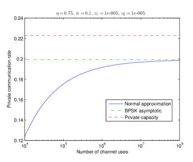
(a)

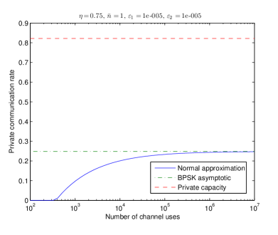
(b)

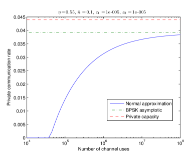
(c)

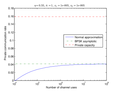
(d)

Figure 1: The figures plot the normal approximation for non-asymptotic BPSK private communication (using (4.90)), the asymptotic limit for BPSK, and the asymptotic energy-constrained private capacity for various values of the channel transmissivity $\eta$, the mean photon number $\bar{n}$, $\varepsilon_{1}$, and $\varepsilon_{2}$.

5 Conclusion

This paper establishes a lower bound on the $\varepsilon$-one-shot private classical capacity of a cq wiretap channel, which in turn leads to a lower bound on the second-order coding rate for private communication over an i.i.d. cq wiretap channel. The main techniques used are position-based decoding [AJW17] in order to guarantee that Bob can decode reliably and convex splitting [ADJ17] to guarantee that Eve cannot determine which message Alice transmitted. It is my opinion that these two methods represent a powerful approach to quantum information theory, having already been used effectively in a variety of contexts in [ADJ17, AJW17].

For future work, it would be good to improve upon the lower bounds given here. Extensions of the methods of [YSP16] and [TB16] might be helpful in this endeavor.

Note: After the completion of the results in the present paper, Naqueeb Warsi informed the author of an unpublished result from [War15], which establishes a lower bound on the $\varepsilon$-one-shot private capacity of a cq wiretap channel in terms of a difference of the hypothesis testing mutual information and a smooth max-mutual information.

Acknowledgements. I am grateful to Anurag Anshu, Saikat Guha, Rahul Jain, Haoyu Qi, Qingle Wang, and Naqueeb Warsi for discussions related to the topic of this paper. I acknowledge support from the Office of Naval Research and the National Science Foundation.

Appendix A Proof of convex-split lemma

For the sake of completeness, this appendix features a proof of Lemma 2. Let $\widetilde{\rho}_{AB}$ be the optimizer for

$$\lambda^{\ast}\equiv\widetilde{I}_{\max}^{\sqrt{\varepsilon}-\eta}(B;A)_{\rho}=\inf_{\rho_{AB}^{\prime}\ :\ P(\rho_{AB}^{\prime},\rho_{AB})\leq\sqrt{\varepsilon}-\eta}D_{\max}(\rho_{AB}^{\prime}\|\rho_{A}\otimes\rho_{B}^{\prime}).$$ (A.1)

We take $\widetilde{\rho}_{B}$ as the marginal of $\widetilde{\rho}_{AB}$. We define the following state, which we think of as an approximation to $\tau_{A_{1}\cdots A_{K}B}$:

$$\widetilde{\tau}_{A_{1}\cdots A_{K}B}\equiv\frac{1}{K}\sum_{k=1}^{K}\rho_{A_{1}}\otimes\cdots\otimes\rho_{A_{k-1}}\otimes\widetilde{\rho}_{A_{k}B}\otimes\rho_{A_{k+1}}\otimes\cdots\otimes\rho_{A_{K}}.$$ (A.2)

In fact, it is a good approximation if $\sqrt{\varepsilon}-\eta$ is small: Consider from joint concavity of the root fidelity that

$$\sqrt{F}(\widetilde{\tau}_{A_{1}\cdots A_{K}B},\tau_{A_{1}\cdots A_{K}B})$$

$$\geq\frac{1}{K}\sum_{k=1}^{K}\sqrt{F}(\rho_{A_{1}}\otimes\cdots\otimes\rho_{A_{k-1}}\otimes\widetilde{\rho}_{A_{k}B}\otimes\rho_{A_{k+1}}\otimes\cdots\otimes\rho_{A_{K}},$$

$$\qquad\qquad\qquad\qquad\rho_{A_{1}}\otimes\cdots\otimes\rho_{A_{k-1}}\otimes\rho_{A_{k}B}\otimes\rho_{A_{k+1}}\otimes\cdots\otimes\rho_{A_{K}})$$ (A.3)

$$=\frac{1}{K}\sum_{k=1}^{K}\sqrt{F}(\widetilde{\rho}_{A_{k}B},\rho_{A_{k}B})$$ (A.4)

$$=\sqrt{F}(\widetilde{\rho}_{AB},\rho_{AB}),$$ (A.5)

which in turn implies that

$$F(\widetilde{\tau}_{A_{1}\cdots A_{K}B},\tau_{A_{1}\cdots A_{K}B})\geq F(\widetilde{\rho}_{AB},\rho_{AB}).$$ (A.6)

So the inequality in (A.6), the definition of the purified distance, and the fact that $P(\rho_{AB},\widetilde{\rho}_{AB})\leq\sqrt{\varepsilon}-\eta$ imply that

$$P(\widetilde{\tau}_{A_{1}\cdots A_{K}B},\tau_{A_{1}\cdots A_{K}B})\leq\sqrt{\varepsilon}-\eta.$$ (A.7)

Let $\omega=\sum_{y}p_{Y}(y)\omega^{y}$, for $p_{Y}$ a probability distribution and $\{\omega^{y}\}_{y}$ a set of states. Then the following property holds for quantum relative entropy and a state $\kappa$ such that $\operatorname{supp}(\omega)\subseteq\operatorname{supp}(\kappa)$:

$$D(\omega\|\kappa)=\sum_{y}p_{Y}(y)\left[D(\omega^{y}\|\kappa)-D(\omega^{y}\|\omega)\right].$$ (A.8)

Applying (A.8), it follows that

$$D(\widetilde{\tau}_{A_{1}\cdots A_{K}B}\|\rho_{A_{1}}\otimes\cdots\otimes\rho_{A_{K}}\otimes\widetilde{\rho}_{B})\\ =\frac{1}{K}\sum_{k=1}^{K}D(\rho_{A_{1}}\otimes\cdots\otimes\rho_{A_{k-1}}\otimes\rho_{A_{k}B}\otimes\rho_{A_{k+1}}\otimes\cdots\otimes\rho_{A_{K}}\|\rho_{A_{1}}\otimes\cdots\otimes\rho_{A_{K}}\otimes\widetilde{\rho}_{B})\\ -\frac{1}{K}\sum_{k=1}^{K}D(\rho_{A_{1}}\otimes\cdots\otimes\rho_{A_{k-1}}\otimes\rho_{A_{k}B}\otimes\rho_{A_{k+1}}\otimes\cdots\otimes\rho_{A_{K}}\|\widetilde{\tau}_{A_{1}\cdots A_{K}B}).$$ (A.9)

The first term in (A.9) on the right-hand side of the equality simplifies as

$$\frac{1}{K}\sum_{k=1}^{K}D(\rho_{A_{1}}\otimes\cdots\otimes\rho_{A_{k-1}}\otimes\rho_{A_{k}B}\otimes\rho_{A_{k+1}}\otimes\cdots\otimes\rho_{A_{K}}\|\rho_{A_{1}}\otimes\cdots\otimes\rho_{A_{K}}\otimes\widetilde{\rho}_{B})$$

$$=\frac{1}{K}\sum_{k=1}^{K}D(\rho_{A_{k}B}\|\rho_{A_{k}}\otimes\widetilde{\rho}_{B})$$ (A.10)

$$=D(\rho_{AB}\|\rho_{A}\otimes\widetilde{\rho}_{B}).$$ (A.11)

We now lower bound the last term in (A.9). Consider that a partial trace over systems $A_{1}$, …, $A_{k-1}$, $A_{k+1}$, …, $A_{K}$ gives

$$D(\rho_{A_{1}}\otimes\cdots\otimes\rho_{A_{k-1}}\otimes\rho_{A_{k}B}\otimes\rho_{A_{k+1}}\otimes\cdots\otimes\rho_{A_{K}}\|\widetilde{\tau}_{A_{1}\cdots A_{K}B})\\ \geq D(\rho_{A_{k}B}\|\widetilde{\tau}_{A_{k}B})=D(\rho_{AB}\|\left[1/K\right]\widetilde{\rho}_{AB}+\left[1-1/K\right]\rho_{A}\otimes\widetilde{\rho}_{B}),$$ (A.12)

where the equality follows because $\widetilde{\tau}_{A_{k}B}=\left[1/K\right]\widetilde{\rho}_{AB}+\left[1-1/K\right]\rho_{A}\otimes\widetilde{\rho}_{B}$. Thus, averaging the inequality in (A.12) over $k$ implies that

$$\frac{1}{K}\sum_{k=1}^{K}D(\rho_{A_{1}}\otimes\cdots\otimes\rho_{A_{k-1}}\otimes\rho_{A_{k}B}\otimes\rho_{A_{k+1}}\otimes\cdots\otimes\rho_{A_{K}}\|\widetilde{\tau}_{A_{1}\cdots A_{K}B})\\ \geq D(\rho_{AB}\|\left[1/K\right]\widetilde{\rho}_{AB}+\left[1-1/K\right]\rho_{A}\otimes\widetilde{\rho}_{B}),$$ (A.13)

Putting together (A.9), (A.11), and (A.13), we find that

$$D(\widetilde{\tau}_{A_{1}\cdots A_{K}B}\|\rho_{A_{1}}\otimes\cdots\otimes\rho_{A_{K}}\otimes\rho_{B})\\ \leq D(\rho_{AB}\|\rho_{A}\otimes\widetilde{\rho}_{B})-D(\rho_{AB}\|\left[1/K\right]\widetilde{\rho}_{AB}+\left[1-1/K\right]\rho_{A}\otimes\widetilde{\rho}_{B})$$ (A.14)

By the definition of $\lambda^{\ast}$ in (A.1), we have that

$$\widetilde{\rho}_{AB}\leq 2^{\lambda^{\ast}}\rho_{A}\otimes\widetilde{\rho}_{B},$$ (A.15)

which means that

$$\left[1/K\right]\widetilde{\rho}_{AB}+\left[1-1/K\right]\rho_{A}\otimes\widetilde{\rho}_{B}\leq\left[1+(2^{\lambda^{\ast}}-1)/K\right]\rho_{A}\otimes\widetilde{\rho}_{B}.$$ (A.16)

An important property of quantum relative entropy is that $D(\omega\|\tau)\geq D(\omega\|\tau^{\prime})$ if $\tau\leq\tau^{\prime}$. Applying it to (A.16) and the right-hand side of (A.14), we get that

$$D(\rho_{AB}\|\rho_{A}\otimes\widetilde{\rho}_{B})-D(\rho_{AB}\|\left[1/K\right]\widetilde{\rho}_{AB}+\left[1-1/K\right]\rho_{A}\otimes\widetilde{\rho}_{B})$$

$$\leq D(\rho_{AB}\|\rho_{A}\otimes\widetilde{\rho}_{B})-D(\rho_{AB}\|\left[1+(2^{\lambda^{\ast}}-1)/K\right]\rho_{A}\otimes\widetilde{\rho}_{B})$$ (A.17)

$$=D(\rho_{AB}\|\rho_{A}\otimes\widetilde{\rho}_{B})-D(\rho_{AB}\|\rho_{A}\otimes\widetilde{\rho}_{B})+\log_{2}\left[1+(2^{\lambda^{\ast}}-1)/K\right]$$ (A.18)

$$=\log_{2}\left[1+(2^{\lambda^{\ast}}-1)/K\right].$$ (A.19)

Then the well known inequality $D(\omega\|\tau)\geq-\log_{2}F(\omega,\tau)$, (A.14), and (A.17)–(A.19) imply that

$$-\log_{2}F(\widetilde{\tau}_{A_{1}\cdots A_{K}B},\rho_{A_{1}}\otimes\cdots\otimes\rho_{A_{K}}\otimes\widetilde{\rho}_{B})\leq\log_{2}\left[1+(2^{\lambda^{\ast}}-1)/K\right],$$ (A.20)

which in turn implies that

$$F(\widetilde{\tau}_{A_{1}\cdots A_{K}B},\rho_{A_{1}}\otimes\cdots\otimes\rho_{A_{K}}\otimes\widetilde{\rho}_{B})\geq\frac{1}{1+\frac{2^{\lambda^{\ast}}-1}{K}}=1-\frac{2^{\lambda^{\ast}}-1}{K+2^{\lambda^{\ast}}-1}\geq 1-\frac{2^{\lambda^{\ast}}}{K}.$$ (A.21)

So if we pick $K$ such that

$$\log_{2}K=\inf_{\rho_{AB}^{\prime}\ :\ P(\rho_{AB}^{\prime},\rho_{AB})\leq\sqrt{\varepsilon}-\eta}D_{\max}(\rho_{AB}^{\prime}\|\rho_{A}\otimes\rho_{B}^{\prime})+2\log_{2}\left(\frac{1}{\eta}\right),$$ (A.22)

then we are guaranteed that

$$P(\widetilde{\tau}_{A_{1}\cdots A_{K}B},\rho_{A_{1}}\otimes\cdots\otimes\rho_{A_{K}}\otimes\widetilde{\rho}_{B})\leq\eta.$$ (A.23)

By the triangle inequality for the purified distance, we then get that

$$P(\tau_{A_{1}\cdots A_{K}B},\rho_{A_{1}}\otimes\cdots\otimes\rho_{A_{K}}\otimes\widetilde{\rho}_{B})$$

$$\leq P(\tau_{A_{1}\cdots A_{K}B},\widetilde{\tau}_{A_{1}\cdots A_{K}B})+P(\widetilde{\tau}_{A_{1}\cdots A_{K}B},\rho_{A_{1}}\otimes\cdots\otimes\rho_{A_{K}}\otimes\widetilde{\rho}_{B})$$ (A.24)

$$\leq\left(\sqrt{\varepsilon}-\eta\right)+\eta=\sqrt{\varepsilon}.$$ (A.25)

This concludes the proof.

References

• [ADJ17] Anurag Anshu, Vamsi Krishna Devabathini, and Rahul Jain. Quantum message compression with applications. February 2017. arXiv:1410.3031v4.
• [AJW17] Anurag Anshu, Rahul Jain, and Naqueeb Ahmad Warsi. One shot entanglement assisted classical and quantum communication over noisy quantum channels: A hypothesis testing and convex split approach. February 2017. arXiv:1702.01940.
• [BB84] Charles H. Bennett and Gilles Brassard. Quantum cryptography: Public key distribution and coin tossing. In Proceedings of IEEE International Conference on Computers Systems and Signal Processing, pages 175–179, Bangalore, India, December 1984.
• [BD10] Francesco Buscemi and Nilanjana Datta. The quantum capacity of channels with arbitrarily correlated noise. IEEE Transactions on Information Theory, 56(3):1447–1460, March 2010. arXiv:0902.0158.
• [BDL16] Salman Beigi, Nilanjana Datta, and Felix Leditzky. Decoding quantum information via the Petz recovery map. Journal of Mathematical Physics, 57(8):082203, August 2016. arXiv:1504.04449.
• [CK78] Imre Csiszár and Janos Körner. Broadcast channels with confidential messages. IEEE Transactions on Information Theory, 24(3):339–348, May 1978.
• [CWY04] Ning Cai, Andreas Winter, and Raymond W. Yeung. Quantum privacy and quantum wiretap channels. Problems of Information Transmission, 40(4):318–336, October 2004.
• [Dat09] Nilanjana Datta. Min- and max-relative entropies and a new entanglement monotone. IEEE Transactions on Information Theory, 55(6):2816–2826, June 2009. arXiv:0803.2770.
• [Dev05] Igor Devetak. The private classical capacity and quantum capacity of a quantum channel. IEEE Transactions on Information Theory, 51(1):44–55, January 2005. arXiv:quant-ph/0304127.
• [DHO16] Nilanjana Datta, Min-Hsiu Hsieh, and Jonathan Oppenheim. An upper bound on the second order asymptotic expansion for the quantum communication cost of state redistribution. Journal of Mathematical Physics, 57(5):052203, May 2016. arXiv:1409.4352.
• [DL15] Nilanjana Datta and Felix Leditzky. Second-order asymptotics for source coding, dense coding, and pure-state entanglement conversions. IEEE Transactions on Information Theory, 61(1):582–608, January 2015. arXiv:1403.2543.
• [DTW16] Nilanjana Datta, Marco Tomamichel, and Mark M. Wilde. On the second-order asymptotics for entanglement-assisted communication. Quantum Information Processing, 15(6):2569–2591, June 2016. arXiv:1405.1797.
• [GGL+04] Vittorio Giovannetti, Saikat Guha, Seth Lloyd, Lorenzo Maccone, Jeffrey H. Shapiro, and Horace P. Yuen. Classical capacity of the lossy bosonic channel: The exact solution. Physical Review Letters, 92(2):027902, January 2004. arXiv:quant-ph/0308012.
• [GLN05] Alexei Gilchrist, Nathan K. Langford, and Michael A. Nielsen. Distance measures to compare real and ideal quantum processes. Physical Review A, 71(6):062310, June 2005. arXiv:quant-ph/0408063.
• [GW12] Saikat Guha and Mark M. Wilde. Polar coding to achieve the Holevo capacity of a pure-loss optical channel. Proceedings of the 2012 IEEE International Symposium on Information Theory, pages 546–550, 2012. arXiv:1202.0533.
• [Hay06] Masahito Hayashi. General nonasymptotic and asymptotic formulas in channel resolvability and identification capacity and their application to the wiretap channel. IEEE Transactions on Information Theory, 52(4):1562–1575, April 2006. arXiv:cs/0503088.
• [Hay13] Masahito Hayashi. Tight exponential analysis of universally composable privacy amplification and its applications. IEEE Transactions on Information Theory, 59(11):7728–7746, November 2013. arXiv:1010.1358.
• [HHHO09] Karol Horodecki, Michal Horodecki, Pawel Horodecki, and Jonathan Oppenheim. General paradigm for distilling classical key from quantum states. IEEE Transactions on Information Theory, 55(4):1898–1929, April 2009. arXiv:quant-ph/0506189.
• [HN03] Masahito Hayashi and Hiroshi Nagaoka. General formulas for capacity of classical-quantum channels. IEEE Transactions on Information Theory, 49(7):1753–1768, July 2003. arXiv:quant-ph/0206186.
• [Li14] Ke Li. Second order asymptotics for quantum hypothesis testing. Annals of Statistics, 42(1):171–189, February 2014. arXiv:1208.1400.
• [PPV10] Yury Polyanskiy, H. Vincent Poor, and Sergio Verdú. Channel coding rate in the finite blocklength regime. IEEE Transactions on Information Theory, 56(5):2307–2359, May 2010.
• [Ras02] Alexey E. Rastegin. Relative error of state-dependent cloning. Physical Review A, 66(4):042304, October 2002.
• [Ras03] Alexey E. Rastegin. A lower bound on the relative error of mixed-state cloning and related operations. Journal of Optics B: Quantum and Semiclassical Optics, 5(6):S647, December 2003. arXiv:quant-ph/0208159.
• [Ras06] Alexey E. Rastegin. Sine distance for quantum states. February 2006. arXiv:quant-ph/0602112.
• [RR11] Joseph M. Renes and Renato Renner. Noisy channel coding via privacy amplification and information reconciliation. IEEE Transactions on Information Theory, 57(11):7377–7385, Nov 2011.
• [Ser17] Alessio Serafini. Quantum Continuous Variables. CRC Press, 2017.
• [Tan12] Vincent Y. F. Tan. Achievable second-order coding rates for the wiretap channel. In 2012 IEEE International Conference on Communication Systems (ICCS), pages 65–69, November 2012.
• [TB16] Mehrdad Tahmasbi and Matthieu R. Bloch. Second order asymptotics for degraded wiretap channels: How good are existing codes? In 2016 54th Annual Allerton Conference on Communication, Control, and Computing (Allerton), pages 830–837, September 2016.
• [TBR16] Marco Tomamichel, Mario Berta, and Joseph M. Renes. Quantum coding with finite resources. Nature Communications, 7:11419, May 2016. arXiv:1504.04617.
• [TCR09] Marco Tomamichel, Roger Colbeck, and Renato Renner. A fully quantum asymptotic equipartition property. IEEE Transactions on Information Theory, 55(12):5840–5847, December 2009. arXiv:0811.1221.
• [TH13] Marco Tomamichel and Masahito Hayashi. A hierarchy of information quantities for finite block length analysis of quantum tasks. IEEE Transactions on Information Theory, 59(11):7693–7710, November 2013. arXiv:1208.1478.
• [TT15] Marco Tomamichel and Vincent Y. F. Tan. Second-order asymptotics for the classical capacity of image-additive quantum channels. Communications in Mathematical Physics, 338(1):103–137, August 2015. arXiv:1308.6503.
• [Uhl76] Armin Uhlmann. The “transition probability” in the state space of a *-algebra. Reports on Mathematical Physics, 9(2):273–279, 1976.
• [Ume62] Hisaharu Umegaki. Conditional expectations in an operator algebra IV (entropy and information). Kodai Mathematical Seminar Reports, 14(2):59–85, 1962.
• [War15] Naqueeb Ahmad Warsi. One-shot bounds in classical and quantum information theory. PhD thesis, Tata Institute of Fundamental Research, Mumbai, India, December 2015. Not publicly available; communicated by email on March 5, 2017.
• [Wil16] Mark M. Wilde. From Classical to Quantum Shannon Theory. March 2016. arXiv:1106.1445v7.
• [WQ16] Mark M. Wilde and Haoyu Qi. Energy-constrained private and quantum capacities of quantum channels. September 2016. arXiv:1609.01997.
• [WR12] Ligong Wang and Renato Renner. One-shot classical-quantum capacity and hypothesis testing. Physical Review Letters, 108(20):200501, May 2012. arXiv:1007.5456.
• [WTB17] Mark M. Wilde, Marco Tomamichel, and Mario Berta. Converse bounds for private communication over quantum channels. IEEE Transactions on Information Theory, 63(3):1792–1817, March 2017. arXiv:1602.08898.
• [Wyn75] Aaron D. Wyner. The wire-tap channel. Bell System Technical Journal, 54(8):1355–1387, October 1975.
• [YAG13] Mohammad Hossein Yassaee, Mohammad Reza Aref, and Amin Gohari. Non-asymptotic output statistics of random binning and its applications. In 2013 IEEE International Symposium on Information Theory, pages 1849–1853, July 2013. arXiv:1303.0695.
• [YSP16] Wei Yang, Rafael F. Schaefer, and H. Vincent Poor. Finite-blocklength bounds for wiretap channels. In 2016 IEEE International Symposium on Information Theory (ISIT), pages 3087–3091, July 2016. arXiv:1601.06055.