Measuring Sample Quality with Kernels

Abstract

Approximate Markov chain Monte Carlo (MCMC) offers the promise of more rapid sampling at the cost of more biased inference. Since standard MCMC diagnostics fail to detect these biases, researchers have developed computable Stein discrepancy measures that provably determine the convergence of a sample to its target distribution. This approach was recently combined with the theory of reproducing kernels to define a closed-form kernel Stein discrepancy (KSD) computable by summing kernel evaluations across pairs of sample points. We develop a theory of weak convergence for KSDs based on Stein’s method, demonstrate that commonly used KSDs fail to detect non-convergence even for Gaussian targets, and show that kernels with slowly decaying tails provably determine convergence for a large class of target distributions. The resulting convergence-determining KSDs are suitable for comparing biased, exact, and deterministic sample sequences and simpler to compute and parallelize than alternative Stein discrepancies. We use our tools to compare biased samplers, select sampler hyperparameters, and improve upon existing KSD approaches to one-sample hypothesis testing and sample quality improvement.

1 Introduction

When Bayesian inference and maximum likelihood estimation (Geyer, 1991) demand the evaluation of intractable expectations $\mathbb{E}_{P}\mathopen{}\mathclose{{}\left[{h({Z})}}\right]=\int p(x)h(x)dx$ under a target distribution $P$, Markov chain Monte Carlo (MCMC) methods (Brooks et al., 2011) are often employed to approximate these integrals with asymptotically correct sample averages $\mathbb{E}_{Q_{n}}\mathopen{}\mathclose{{}\left[{h({X})}}\right]=\frac{1}{n}\sum_{i=1}^{n}h(x_{i})$. However, many exact MCMC methods are computationally expensive, and recent years have seen the introduction of biased MCMC procedures (see, e.g., Welling & Teh, 2011; Ahn et al., 2012; Korattikara et al., 2014) that exchange asymptotic correctness for increased sampling speed.

Since standard MCMC diagnostics, like mean and trace plots, pooled and within-chain variance measures, effective sample size, and asymptotic variance (Brooks et al., 2011), do not account for asymptotic bias, Gorham & Mackey (2015) defined a new family of sample quality measures – the Stein discrepancies – that measure how well $\mathbb{E}_{Q_{n}}$ approximates $\mathbb{E}_{P}$ while avoiding explicit integration under $P$. Gorham & Mackey (2015); Mackey & Gorham (2016); Gorham et al. (2016) further showed that specific members of this family – the graph Stein discrepancies – were (a) efficiently computable by solving a linear program and (b) convergence-determining for large classes of targets $P$. Building on the zero mean reproducing kernel theory of Oates et al. (2016b), Chwialkowski et al. (2016) and Liu et al. (2016) later showed that other members of the Stein discrepancy family had a closed-form solution involving the sum of kernel evaluations over pairs of sample points.

This closed form represents a significant practical advantage, as no linear program solvers are necessary, and the computation of the discrepancy can be easily parallelized. However, as we will see in Section 3.2, not all kernel Stein discrepancies are suitable for our setting. In particular, in dimension $d\geq 3$, the kernel Stein discrepancies previously recommended in the literature fail to detect when a sample is not converging to the target. To address this shortcoming, we develop a theory of weak convergence for the kernel Stein discrepancies analogous to that of (Gorham & Mackey, 2015; Mackey & Gorham, 2016; Gorham et al., 2016) and design a class of kernel Stein discrepancies that provably control weak convergence for a large class of target distributions.

After formally describing our goals for measuring sample quality in Section 2, we outline our strategy, based on Stein’s method, for constructing and analyzing practical quality measures at the start of Section 3. In Section 3.1, we define our family of closed-form quality measures – the kernel Stein discrepancies (KSDs) – and establish several appealing practical properties of these measures. We analyze the convergence properties of KSDs in Sections 3.2 and 3.3, showing that previously proposed KSDs fail to detect non-convergence and proposing practical convergence-determining alternatives. Section 4 illustrates the value of convergence-determining kernel Stein discrepancies in a variety of applications, including hyperparameter selection, sampler selection, one-sample hypothesis testing, and sample quality improvement. Finally, in Section 5, we conclude with a discussion of related and future work.

Notation We will use $\mu$ to denote a generic probability measure and $\Rightarrow$ to denote the weak convergence of a sequence of probability measures. We will use $\mathopen{}\mathclose{{}\left\|{\cdot}}\right\|_{r}$ for $r\in[1,\infty]$ to represent the $\ell^{r}$ norm on $\mathbb{R}^{d}$ and occasionally refer to a generic norm $\mathopen{}\mathclose{{}\left\|{\cdot}}\right\|$ with associated dual norm $\mathopen{}\mathclose{{}\left\|{a}}\right\|^{*}\triangleq\sup_{b\in\mathbb{R}^{d},\mathopen{}\mathclose{{}\left\|{b}}\right\|=1}{\langle{a},{b}\rangle}$ for vectors $a\in\mathbb{R}^{d}$. We let $e_{j}$ be the $j$-th standard basis vector. For any function $g:\mathbb{R}^{d}\to\mathbb{R}^{d^{\prime}}$, we define $M_{0}(g)\triangleq\sup_{x\in\mathbb{R}^{d}}\mathopen{}\mathclose{{}\left\|{g(x)}}\right\|_{2}$, $M_{1}(g)\triangleq\sup_{x\neq y}\mathopen{}\mathclose{{}\left\|{g(x)-g(y)}}\right\|_{2}/\mathopen{}\mathclose{{}\left\|{x-y}}\right\|_{2}$, and $\nabla g$ as the gradient with components $(\nabla g(x))_{jk}\triangleq\nabla_{x_{k}}g_{j}(x)$. We further let $g\in C^{m}$ indicate that $g$ is $m$ times continuously differentiable and $g\in C_{0}^{m}$ indicate that $g\in C^{m}$ and $\nabla^{l}g$ is vanishing at infinity for all $l\in\{0,\dots,m\}$. We define $C^{(m,m)}$ (respectively, $C_{b}^{(m,m)}$ and $C_{0}^{(m,m)}$) to be the set of functions $k:\mathbb{R}^{d}\times\mathbb{R}^{d}\to\mathbb{R}$ with $(x,y)\mapsto\nabla_{x}^{l}\nabla_{y}^{l}k(x,y)$ continuous (respectively, continuous and uniformly bounded, continuous and vanishing at infinity) for all $l\in\{0,\dots,m\}$.

2 Quality measures for samples

Consider a target distribution $P$ with continuously differentiable (Lebesgue) density $p$ supported on all of $\mathbb{R}^{d}$. We assume that the score function $b\triangleq\nabla\log p$ can be evaluated but that, for most functions of interest, direct integration under $P$ is infeasible. We will therefore approximate integration under $P$ using a weighted sample $Q_{n}=\sum_{i=1}^{n}q_{n}(x_{i})\delta_{x_{i}}$ with sample points $x_{1},\dots,x_{n}\in\mathbb{R}^{d}$ and $q_{n}$ a probability mass function. We will make no assumptions about the origins of the sample points; they may be the output of a Markov chain or even deterministically generated.

Each $Q_{n}$ offers an approximation $\mathbb{E}_{Q_{n}}\mathopen{}\mathclose{{}\left[{h({X})}}\right]=\sum_{i=1}^{n}q_{n}(x_{i})h(x_{i})$ for each intractable expectation $\mathbb{E}_{P}\mathopen{}\mathclose{{}\left[{h({Z})}}\right]$, and our aim is to effectively compare the quality of the approximation offered by any two samples targeting $P$. In particular, we wish to produce a quality measure that (i) identifies when a sequence of samples is converging to the target, (ii) determines when a sequence of samples is not converging to the target, and (iii) is efficiently computable. Since our interest is in approximating expectations, we will consider discrepancies quantifying the maximum expectation error over a class of test functions $\mathcal{H}$:

$$d_{\mathcal{H}}(Q_{n},P)\triangleq\sup_{h\in\mathcal{H}}|\mathbb{E}_{P}\mathopen{}\mathclose{{}\left[{h({Z})}}\right]-\mathbb{E}_{Q_{n}}\mathopen{}\mathclose{{}\left[{h({X})}}\right]|.$$ (1)

When $\mathcal{H}$ is large enough, for any sequence of probability measures $(\mu_{m})_{m\geq 1}$, $d_{\mathcal{H}}(\mu_{m},P)\to 0$ only if $\mu_{m}\Rightarrow P$. In this case, we call (1) an integral probability metric (IPM) (Müller, 1997). For example, when $\mathcal{H}=BL_{\mathopen{}\mathclose{{}\left\|{\cdot}}\right\|_{2}}\triangleq\{h:\mathbb{R}^{d}\to\mathbb{R}\,|\,M_{0}(h)+M_{1}(h)\leq 1\}$, the IPM $d_{BL_{\mathopen{}\mathclose{{}\left\|{\cdot}}\right\|_{2}}}$ is called the bounded Lipschitz or Dudley metric and exactly metrizes convergence in distribution. Alternatively, when $\mathcal{H}=\mathcal{W}_{\mathopen{}\mathclose{{}\left\|{\cdot}}\right\|_{2}}\triangleq\{h:\mathbb{R}^{d}\to\mathbb{R}\,|\,M_{1}(h)\leq 1\}$ is the set of $1$-Lipschitz functions, the IPM $d_{\mathcal{W}_{\mathopen{}\mathclose{{}\left\|{\cdot}}\right\|}}$ in (1) is known as the Wasserstein metric.

An apparent practical problem with using the IPM $d_{\mathcal{H}}$ as a sample quality measure is that $\mathbb{E}_{P}\mathopen{}\mathclose{{}\left[{h({Z})}}\right]$ may not be computable for $h\in\mathcal{H}$. However, if $\mathcal{H}$ were chosen such that $\mathbb{E}_{P}\mathopen{}\mathclose{{}\left[{h({Z})}}\right]=0$ for all $h\in\mathcal{H}$, then no explicit integration under $P$ would be necessary. To generate such a class of test functions and to show that the resulting IPM still satisfies our desiderata, we follow the lead of Gorham & Mackey (2015) and consider Charles Stein’s method for characterizing distributional convergence.

3 Stein’s method with kernels

Stein’s method (Stein, 1972) provides a three-step recipe for assessing convergence in distribution:

1. Identify a Stein operator $\mathcal{T}{}$ that maps functions $g:\mathbb{R}^{d}\to\mathbb{R}^{d}$ from a domain $\mathcal{G}$ to real-valued functions $\mathcal{T}{g}$ such that

   $$\mathbb{E}_{P}\mathopen{}\mathclose{{}\left[{(\mathcal{T}{g})({{Z}})}}\right]=0\text{ for all }g\in\mathcal{G}.$$

   For any such Stein operator and Stein set $\mathcal{G}$, Gorham & Mackey (2015) defined the Stein discrepancy as

   $$\mathcal{S}({\mu},{\mathcal{T}{}},{\mathcal{G}})\triangleq\sup_{g\in\mathcal{G}}|\mathbb{E}_{\mu}\mathopen{}\mathclose{{}\left[{(\mathcal{T}{g})({{X}})}}\right]|=d_{\mathcal{T}{\mathcal{G}}}(\mu,P)$$ (2)

   which, crucially, avoids explicit integration under $P$.

2. Lower bound the Stein discrepancy by an IPM $d_{\mathcal{H}}$ known to dominate weak convergence. This can be done once for a broad class of target distributions to ensure that $\mu_{m}\Rightarrow P$ whenever $\mathcal{S}({\mu_{m}},{\mathcal{T}{}},{\mathcal{G}})\to 0$ for a sequence of probability measures $(\mu_{m})_{m\geq 1}$ (Desideratum (ii)).

3. Provide an upper bound on the Stein discrepancy ensuring that $\mathcal{S}({\mu_{m}},{\mathcal{T}{}},{\mathcal{G}})\to 0$ under suitable convergence of $\mu_{m}$ to $P$ (Desideratum (i)).

While Stein’s method is principally used as a mathematical tool to prove convergence in distribution, we seek, in the spirit of (Gorham & Mackey, 2015; Gorham et al., 2016), to harness the Stein discrepancy as a practical tool for measuring sample quality. The subsections to follow develop a specific, practical instantiation of the abstract Stein’s method recipe based on reproducing kernel Hilbert spaces. An empirical analysis of the Stein discrepancies recommended by our theory follows in Section 4.

3.1 Selecting a Stein operator and a Stein set

A standard, widely applicable univariate Stein operator is the density method operator (see Stein et al., 2004; Chatterjee & Shao, 2011; Chen et al., 2011; Ley et al., 2017),

$$\textstyle(\mathcal{T}{g})({x})\triangleq\frac{1}{p(x)}\frac{d}{dx}(p(x)g(x))=g(x)b(x)+g^{\prime}(x).$$

Inspired by the generator method of Barbour (1988, 1990) and Götze (1991), Gorham & Mackey (2015) generalized this operator to multiple dimensions. The resulting Langevin Stein operator

$$\textstyle(\mathcal{T}_{P}{g})({x})\triangleq\frac{1}{p(x)}\langle{\nabla},{p(x)g(x)}\rangle=\langle{g(x)},{b(x)}\rangle+\langle{\nabla},{g(x)}\rangle$$

for functions $g:\mathbb{R}^{d}\to\mathbb{R}^{d}$ was independently developed, without connection to Stein’s method, by Oates et al. (2016b) for the design of Monte Carlo control functionals. Notably, the Langevin Stein operator depends on $P$ only through its score function $b=\nabla\log p$ and hence is computable even when the normalizing constant of $p$ is not. While our work is compatible with other practical Stein operators, like the family of diffusion Stein operators defined in (Gorham et al., 2016), we will focus on the Langevin operator for the sake of brevity.

Hereafter, we will let $k:\mathbb{R}^{d}\times\mathbb{R}^{d}\to\mathbb{R}$ be the reproducing kernel of a reproducing kernel Hilbert space (RKHS) $\mathcal{K}_{k}$ of functions from $\mathbb{R}^{d}\to\mathbb{R}$. That is, $\mathcal{K}_{k}$ is a Hilbert space of functions such that, for all $x\in\mathbb{R}^{d}$, $k(x,\cdot)\in\mathcal{K}_{k}$ and $f(x)=\langle{f},{k(x,\cdot)}\rangle_{\mathcal{K}_{k}}$ whenever $f\in\mathcal{K}_{k}$. We let $\mathopen{}\mathclose{{}\left\|{\cdot}}\right\|_{\mathcal{K}_{k}}$ be the norm induced from the inner product on $\mathcal{K}_{k}$.

With this definition, we define our kernel Stein set $\mathcal{G}_{k,\mathopen{}\mathclose{{}\left\|{\cdot}}\right\|}$ as the set of vector-valued functions $g=(g_{1},\dots,g_{d})$ such that each component function $g_{j}$ belongs to $\mathcal{K}_{k}$ and the vector of their norms $\mathopen{}\mathclose{{}\left\|{g_{j}}}\right\|_{\mathcal{K}_{k}}$ belongs to the $\mathopen{}\mathclose{{}\left\|{\cdot}}\right\|^{*}$ unit ball:

$$\mathcal{G}_{k,\mathopen{}\mathclose{{}\left\|{\cdot}}\right\|}\triangleq\{g=(g_{1},\dots,g_{d})\mid\mathopen{}\mathclose{{}\left\|{v}}\right\|^{*}\leq 1\text{ for }v_{j}\triangleq\mathopen{}\mathclose{{}\left\|{g_{j}}}\right\|_{\mathcal{K}_{k}}\}.$$

The following result, proved in Section B, establishes that this is an acceptable domain for $\mathcal{T}_{P}{}$.

Proposition 1 (Zero mean test functions).

If $k\in C_{b}^{(1,1)}$ and $\mathbb{E}_{P}\mathopen{}\mathclose{{}\left[{\mathopen{}\mathclose{{}\left\|{\nabla\log p(Z)}}\right\|_{2}}}\right]<\infty$, then $\mathbb{E}_{P}\mathopen{}\mathclose{{}\left[{(\mathcal{T}_{P}{g})({Z})}}\right]=0$ for all $g\in\mathcal{G}_{k,\mathopen{}\mathclose{{}\left\|{\cdot}}\right\|}$.

The Langevin Stein operator and kernel Stein set together define our quality measure of interest, the kernel Stein discrepancy (KSD) $\mathcal{S}({\mu},{\mathcal{T}_{P}{}},{\mathcal{G}_{k,\mathopen{}\mathclose{{}\left\|{\cdot}}\right\|}})$. When $\mathopen{}\mathclose{{}\left\|{\cdot}}\right\|=\mathopen{}\mathclose{{}\left\|{\cdot}}\right\|_{2}$, this definition recovers the KSD proposed by Chwialkowski et al. (2016) and Liu et al. (2016). Our next result shows that, for any $\mathopen{}\mathclose{{}\left\|{\cdot}}\right\|$, the KSD admits a closed-form solution.

Proposition 2 (KSD closed form).

Suppose $k\in C^{(1,1)}$, and, for each $j\in\{1,\dots d\}$, define the Stein kernel

$$k_{0}^{j}(x,y) \triangleq{\textstyle\frac{1}{p(x)p(y)}}\nabla_{x_{j}}\nabla_{y_{j}}(p(x)k(x,y)p(y))$$ (3)

$$=b_{j}(x)b_{j}(y)k(x,y)+b_{j}(x)\nabla_{y_{j}}k(x,y)$$

$$\quad+b_{j}(y)\nabla_{x_{j}}k(x,y)+\nabla_{x_{j}}\nabla_{y_{j}}k(x,y).$$

If $\sum_{j=1}^{d}\mathbb{E}_{\mu}\mathopen{}\mathclose{{}\left[{{k_{0}^{j}(X,X)}^{1/2}}}\right]<\infty$, then $\mathcal{S}({\mu},{\mathcal{T}_{P}{}},{\mathcal{G}_{k,\mathopen{}\mathclose{{}\left\|{\cdot}}\right\|}})=\mathopen{}\mathclose{{}\left\|{w}}\right\|$ where $w_{j}\triangleq\sqrt{\mathbb{E}_{\mu\times\mu}[k_{0}^{j}(X,\tilde{X})}]$ with $X,\tilde{X}\stackrel{{\scriptstyle\mathrm{iid}}}{{\sim}}\mu$.

The proof is found in Section C. Notably, when $\mu$ is the discrete measure $Q_{n}=\sum_{i=1}^{n}q_{n}(x_{i})\delta_{x_{i}}$, the KSD reduces to evaluating each $k_{0}^{j}$ at pairs of support points as $w_{j}=\sqrt{\sum_{i,i^{\prime}=1}^{n}q_{n}(x_{i})k_{0}^{j}(x_{i},x_{i^{\prime}})q_{n}(x_{i^{\prime}})},$ a computation which is easily parallelized over sample pairs and coordinates $j$.

Our Stein set choice was motivated by the work of Oates et al. (2016b) who used the sum of Stein kernels $k_{0}=\sum_{j=1}^{d}k_{0}^{j}$ to develop nonparametric control variates. Each term $w_{j}$ in Proposition 2 can also be viewed as an instance of the maximum mean discrepancy (MMD) (Gretton et al., 2012) between $\mu$ and $P$ measured with respect to the Stein kernel $k_{0}^{j}$. In standard uses of MMD, an arbitrary kernel function is selected, and one must be able to compute expectations of the kernel function under $P$. Here, this requirement is satisfied automatically, since our induced kernels are chosen to have mean zero under $P$.

For clarity we will focus on the specific kernel Stein set choice $\mathcal{G}_{k}\triangleq\mathcal{G}_{k,\mathopen{}\mathclose{{}\left\|{\cdot}}\right\|_{2}}$ for the remainder of the paper, but our results extend directly to KSDs based on any $\mathopen{}\mathclose{{}\left\|{\cdot}}\right\|$, since all KSDs are equivalent in a strong sense:

Proposition 3 (Kernel Stein set equivalence).

Under the assumptions of Proposition 2, there are constants $c_{d},c_{d}^{\prime}>0$ depending only on $d$ and $\mathopen{}\mathclose{{}\left\|{\cdot}}\right\|$ such that $c_{d}\mathcal{S}({\mu},{\mathcal{T}_{P}{}},{\mathcal{G}_{k,\mathopen{}\mathclose{{}\left\|{\cdot}}\right\|}})\leq\mathcal{S}({\mu},{\mathcal{T}_{P}{}},{\mathcal{G}_{k,\mathopen{}\mathclose{{}\left\|{\cdot}}\right\|_{2}}})\leq c_{d}^{\prime}\mathcal{S}({\mu},{\mathcal{T}_{P}{}},{\mathcal{G}_{k,\mathopen{}\mathclose{{}\left\|{\cdot}}\right\|}})$.

The short proof is found in Section D.

3.2 Lower bounding the kernel Stein discrepancy

We next aim to establish conditions under which the KSD $\mathcal{S}({\mu_{m}},{\mathcal{T}_{P}{}},{\mathcal{G}_{k}})\to 0$ only if $\mu_{m}\Rightarrow P$ (Desideratum (ii)). Recently, Gorham et al. (2016) showed that the Langevin graph Stein discrepancy dominates convergence in distribution whenever $P$ belongs to the class $\mathcal{P}$ of distantly dissipative distributions with Lipschitz score function $b$:

Definition 4 (Distant dissipativity (Eberle, 2015; Gorham et al., 2016)).

A distribution $P$ is distantly dissipative if $\kappa_{0}\triangleq\lim\inf_{r\to\infty}\kappa(r)>0$ for

$$\kappa(r)=\inf\{-2{\textstyle\frac{\langle{b(x)-b(y)},{x-y}\rangle}{\mathopen{}\mathclose{{}\left\|{x-y}}\right\|_{2}^{2}}}:\mathopen{}\mathclose{{}\left\|{x-y}}\right\|_{2}=r\}.$$ (4)

Examples of distributions in $\mathcal{P}$ include finite Gaussian mixtures with common covariance and all distributions strongly log-concave outside of a compact set, including Bayesian linear, logistic, and Huber regression posteriors with Gaussian priors (see Gorham et al., 2016, Section 4). Moreover, when $d=1$, membership in $\mathcal{P}$ is sufficient to provide a lower bound on the KSD for most common kernels including the Gaussian, Matérn, and inverse multiquadric kernels.

Theorem 5 (Univariate KSD detects non-convergence).

Suppose that $P\in\mathcal{P}$ and $k(x,y)=\Phi(x-y)$ for $\Phi\in C^{2}$ with a non-vanishing generalized Fourier transform. If $d=1$, then $\mathcal{S}({\mu_{m}},{\mathcal{T}_{P}{}},{\mathcal{G}_{k}})\to 0$ only if $\mu_{m}\Rightarrow P$.

The proof in Section E provides a lower bound on the KSD in terms of an IPM known to dominate weak convergence. However, our next theorem shows that in higher dimensions $\mathcal{S}({Q_{n}},{\mathcal{T}_{P}{}},{\mathcal{G}_{k}})$ can converge to $0$ without the sequence $(Q_{n})_{n\geq 1}$ converging to any probability measure. This deficiency occurs even when the target is Gaussian.

Theorem 6 (KSD fails with light kernel tails).

Suppose $k\in C_{b}^{(1,1)}$ and define the kernel decay rate

$$\gamma(r)\triangleq\sup\{\max( |k(x,y)|,\mathopen{}\mathclose{{}\left\|{\nabla_{x}k(x,y)}}\right\|_{2},$$

$$|\langle{\nabla_{x}},{\nabla_{y}k(x,y)}\rangle|):\mathopen{}\mathclose{{}\left\|{x-y}}\right\|_{2}\geq r\}.$$

If $d\geq 3$, $P=\mathcal{N}(0,I_{d})$, and $\gamma(r)=o(r^{-\alpha})$ for $\alpha\triangleq(\frac{1}{2}-\frac{1}{d})^{-1}$, then $\mathcal{S}({Q_{n}},{\mathcal{T}_{P}{}},{\mathcal{G}_{k}})\to 0$ does not imply $Q_{n}\Rightarrow P$.

Theorem 6 implies that KSDs based on the commonly used Gaussian kernel, Matérn kernel, and compactly supported kernels of Wendland (2004, Theorem 9.13) all fail to detect non-convergence when $d\geq 3$. In addition, KSDs based on the inverse multiquadric kernel ($k(x,y)=(c^{2}+\mathopen{}\mathclose{{}\left\|{x-y}}\right\|_{2}^{2})^{\beta}$) for $\beta<-1$ fail to detect non-convergence for any $d>2\beta/(\beta+1)$. The proof in Section F shows that the violating sample sequences $(Q_{n})_{n\geq 1}$ are simple to construct, and we provide an empirical demonstration of this failure to detect non-convergence in Section 4.

The failure of the KSDs in Theorem 6 can be traced to their inability to enforce uniform tightness. A sequence of probability measures $(\mu_{m})_{m\geq 1}$ is uniformly tight if for every $\epsilon>0$, there is a finite number $R(\epsilon)$ such that $\lim\sup_{m}\mu_{m}(\mathopen{}\mathclose{{}\left\|{{X}}}\right\|_{2}>R(\epsilon))\leq\epsilon$. Uniform tightness implies that no mass in the sequence of probability measures escapes to infinity. When the kernel $k$ decays more rapidly than the score function grows, the KSD ignores excess mass in the tails and hence can be driven to zero by a non-tight sequence of increasingly diffuse probability measures. The following theorem demonstrates uniform tightness is the missing piece to ensure weak convergence.

Theorem 7 (KSD detects tight non-convergence).

Suppose that $P\in\mathcal{P}$ and $k(x,y)=\Phi(x-y)$ for $\Phi\in C^{2}$ with a non-vanishing generalized Fourier transform. If $(\mu_{m})_{m\geq 1}$ is uniformly tight, then $\mathcal{S}({\mu_{m}},{\mathcal{T}_{P}{}},{\mathcal{G}_{k}})\to 0$ only if $\mu_{m}\Rightarrow P$.

Our proof in Section G explicitly lower bounds the KSD $\mathcal{S}({\mu},{\mathcal{T}_{P}{}},{\mathcal{G}_{k}})$ in terms of the bounded Lipschitz metric $d_{BL_{\mathopen{}\mathclose{{}\left\|{\cdot}}\right\|}}(\mu,P)$, which exactly metrizes weak convergence.

Ideally, when a sequence of probability measures is not uniformly tight, the KSD would reflect this divergence in its reported value. To achieve this, we consider the inverse multiquadric (IMQ) kernel $k(x,y)=(c^{2}+\mathopen{}\mathclose{{}\left\|{x-y}}\right\|_{2}^{2})^{\beta}\,$ for some $\beta<0$ and $c>0$. While KSDs based on IMQ kernels fail to determine convergence when $\beta<-1$ (by Theorem 6), our next theorem shows that they automatically enforce tightness and detect non-convergence whenever $\beta\in(-1,0)$.

Theorem 8 (IMQ KSD detects non-convergence).

Suppose $P\in\mathcal{P}$ and $k(x,y)=(c^{2}+\mathopen{}\mathclose{{}\left\|{x-y}}\right\|_{2}^{2})^{\beta}$ for $c>0$ and $\beta\in(-1,0)$. If $\mathcal{S}({\mu_{m}},{\mathcal{T}_{P}{}},{\mathcal{G}_{k}})\to 0$, then $\mu_{m}\Rightarrow P$.

The proof in Section H provides a lower bound on the KSD in terms of the bounded Lipschitz metric $d_{BL_{\mathopen{}\mathclose{{}\left\|{\cdot}}\right\|}}(\mu,P)$. The success of the IMQ kernel over other common characteristic kernels can be attributed to its slow decay rate. When $P\in\mathcal{P}$ and the IMQ exponent $\beta>-1$, the function class $\mathcal{T}_{P}{\mathcal{G}_{k}}$ contains unbounded (coercive) functions. These functions ensure that the IMQ KSD $\mathcal{S}({\mu_{m}},{\mathcal{T}_{P}{}},{\mathcal{G}_{k}})$ goes to $0$ only if $(\mu_{m})_{m\geq 1}$ is uniformly tight.

3.3 Upper bounding the kernel Stein discrepancy

The usual goal in upper bounding the Stein discrepancy is to provide a rate of convergence to $P$ for particular approximating sequences $(\mu_{m})_{m=1}^{\infty}$. Because we aim to directly compute the KSD for arbitrary samples $Q_{n}$, our chief purpose in this section is to ensure that the KSD $\mathcal{S}({\mu_{m}},{\mathcal{T}_{P}{}},{\mathcal{G}_{k}})$ will converge to zero when $\mu_{m}$ is converging to $P$ (Desideratum (i)).

Proposition 9 (KSD detects convergence).

If $k\in C_{b}^{(2,2)}$ and $\nabla\log p$ is Lipschitz with $\mathbb{E}_{P}[\mathopen{}\mathclose{{}\left\|{\nabla\log p(Z)}}\right\|_{2}^{2}]<\infty$, then $\mathcal{S}({\mu_{m}},{\mathcal{T}_{P}{}},{\mathcal{G}_{k}})\to 0$ whenever the Wasserstein distance $d_{\mathcal{W}_{\mathopen{}\mathclose{{}\left\|{\cdot}}\right\|_{2}}}(\mu_{m},P)\to 0$.

Proposition 9 applies to common kernels like the Gaussian, Matérn, and IMQ kernels, and its proof in Section I provides an explicit upper bound on the KSD in terms of the Wasserstein distance $d_{\mathcal{W}_{\mathopen{}\mathclose{{}\left\|{\cdot}}\right\|_{2}}}$. When $Q_{n}=\frac{1}{n}\sum_{i=1}^{n}\delta_{x_{i}}$ for $x_{i}\stackrel{{\scriptstyle\mathrm{iid}}}{{\sim}}\mu$, (Liu et al., 2016, Thm. 4.1) further implies that $\mathcal{S}({Q_{n}},{\mathcal{T}_{P}{}},{\mathcal{G}_{k}})\Rightarrow\mathcal{S}({\mu},{\mathcal{T}_{P}{}},{\mathcal{G}_{k}})$ at an $O(n^{-1/2})$ rate under continuity and integrability assumptions on $\mu$.

4 Experiments

We next conduct an empirical evaluation of the KSD quality measures recommended by our theory, recording all timings on an Intel Xeon CPU E5-2650 v2 @ 2.60GHz. Throughout, we will refer to the KSD with IMQ base kernel $k(x,y)=(c^{2}+\mathopen{}\mathclose{{}\left\|{x-y}}\right\|_{2}^{2})^{\beta}$, exponent $\beta=-\frac{1}{2}$, and $c=1$ as the IMQ KSD. Code reproducing all experiments can be found on the Julia (Bezanson et al., 2014) package site https://jgorham.github.io/SteinDiscrepancy.jl/.

4.1 Comparing discrepancies

Our first, simple experiment is designed to illustrate several properties of the IMQ KSD and to compare its behavior with that of two preexisting discrepancy measures, the Wasserstein distance $d_{\mathcal{W}_{\mathopen{}\mathclose{{}\left\|{\cdot}}\right\|_{2}}}$, which can be computed for simple univariate targets (Vallender, 1974), and the spanner graph Stein discrepancy of Gorham & Mackey (2015). We adopt a bimodal Gaussian mixture with $p(x)\propto e^{-\frac{1}{2}\mathopen{}\mathclose{{}\left\|{x+\Delta e_{1}}}\right\|_{2}^{2}}+e^{-\frac{1}{2}\mathopen{}\mathclose{{}\left\|{x-\Delta e_{1}}}\right\|_{2}^{2}}$ and $\Delta=1.5$ as our target $P$ and generate a first sample point sequence i.i.d. from the target and a second sequence i.i.d. from one component of the mixture, $\mathcal{N}(-\Delta e_{1},I_{d})$. As seen in the left panel of Figure 1 where $d=1$, the IMQ KSD decays at an $n^{-0.51}$ rate when applied to the first $n$ points in the target sample and remains bounded away from zero when applied to the to the single component sample. This desirable behavior is closely mirrored by the Wasserstein distance and the graph Stein discrepancy.

The middle panel of Figure 1 records the time consumed by the graph and kernel Stein discrepancies applied to the i.i.d. sample points from $P$. Each method is given access to $d$ cores when working in $d$ dimensions, and we use the released code of Gorham & Mackey (2015) with the default Gurobi 6.0.4 linear program solver for the graph Stein discrepancy. We find that the two methods have nearly identical runtimes when $d=1$ but that the KSD is $10$ to $1000$ times faster when $d=4$. In addition, the KSD is straightforwardly parallelized and does not require access to a linear program solver, making it an appealing practical choice for a quality measure.

Finally, the right panel displays the optimal Stein functions, $g_{j}(y)=\frac{\mathbb{E}_{Q_{n}}\mathopen{}\mathclose{{}\left[{b_{j}(X)k(X,y)+\nabla_{x_{j}}k(X,y)}}\right]}{\mathcal{S}({Q_{n}},{\mathcal{T}_{P}{}},{\mathcal{G}_{k}})}$, recovered by the IMQ KSD when $d=1$ and $n=10^{3}$. The associated test functions $h(y)=(\mathcal{T}_{P}{g})({y})=\frac{\sum_{j=1}^{d}\mathbb{E}_{Q_{n}}\mathopen{}\mathclose{{}\left[{k_{0}^{j}(X,y)}}\right]}{\mathcal{S}({Q_{n}},{\mathcal{T}_{P}{}},{\mathcal{G}_{k}})}$ are the mean-zero functions under $P$ that best discriminate the target $P$ and the sample $Q_{n}$. The optimal test function for the single component sample features large positive values in the oversampled region that fail to be offset by negative values in the undersampled region near the missing mode.

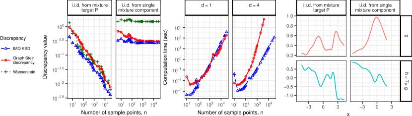
Figure 1: Left: For $d=1$, comparison of discrepancy measures for samples drawn i.i.d. from either the bimodal Gaussian mixture target $P$ or a single mixture component (see Section 4.1). Middle: On-target discrepancy computation time using $d$ cores in $d$ dimensions. Right: For $n=10^{3}$ and $d=1$, the Stein functions $g$ and discriminating test functions $h=\mathcal{T}_{P}{g}$ which maximize the KSD.

4.2 The importance of kernel choice

Theorem 6 established that kernels with rapidly decaying tails yield KSDs that can be driven to zero by off-target sample sequences. Our next experiment provides an empirical demonstration of this issue for a multivariate Gaussian target $P=\mathcal{N}(0,I_{d})$ and KSDs based on the popular Gaussian ($k(x,y)=e^{-\mathopen{}\mathclose{{}\left\|{x-y}}\right\|_{2}^{2}/2}$) and Matérn ($k(x,y)=(1+\sqrt{3}\mathopen{}\mathclose{{}\left\|{x-y}}\right\|_{2})e^{-\sqrt{3}\mathopen{}\mathclose{{}\left\|{x-y}}\right\|_{2}}$) radial kernels.

Following the proof Theorem 6 in Section F, we construct an off-target sequence $(Q_{n})_{n\geq 1}$ that sends $\mathcal{S}({Q_{n}},{\mathcal{T}_{P}{}},{\mathcal{G}_{k}})$ to $0$ for these kernel choices whenever $d\geq 3$. Specifically, for each $n$, we let $Q_{n}=\frac{1}{n}\sum_{i=1}^{n}\delta_{x_{i}}$ where, for all $i$ and $j$, $\mathopen{}\mathclose{{}\left\|{x_{i}}}\right\|_{2}\leq 2n^{1/d}\log n$ and $\mathopen{}\mathclose{{}\left\|{x_{i}-x_{j}}}\right\|_{2}\geq 2\log n$. To select these sample points, we independently sample candidate points uniformly from the ball $\{x:\mathopen{}\mathclose{{}\left\|{x}}\right\|_{2}\leq 2n^{1/d}\log n\}$, accept any points not within $2\log n$ Euclidean distance of any previously accepted point, and terminate when $n$ points have been accepted.

For various dimensions, Figure 2 displays the result of applying each KSD to the off-target sequence $(Q_{n})_{n\geq 1}$ and an “on-target” sequence of points sampled i.i.d. from $P$. For comparison, we also display the behavior of the IMQ KSD which provably controls tightness and dominates weak convergence for this target by Theorem 8. As predicted, the Gaussian and Matérn KSDs decay to $0$ under the off-target sequence and decay more rapidly as the dimension $d$ increases; the IMQ KSD remains bounded away from $0$.

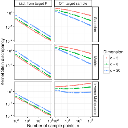
Figure 2: Gaussian and Matérn KSDs are driven to $0$ by an off-target sequence that does not converge to the target $P=\mathcal{N}(0,I_{d})$ (see Section 4.2). The IMQ KSD does not share this deficiency.

4.3 Selecting sampler hyperparameters

The approximate slice sampler of DuBois et al. (2014) is a biased MCMC procedure designed to accelerate inference when the target density takes the form $p(x)\propto\pi(x)\prod_{l=1}^{L}\pi(y_{l}|x)$ for $\pi(\cdot)$ a prior distribution on $\mathbb{R}^{d}$ and $\pi(y_{l}|x)$ the likelihood of a datapoint $y_{l}$. A standard slice sampler must evaluate the likelihood of all $L$ datapoints to draw each new sample point $x_{i}$. To reduce this cost, the approximate slice sampler introduces a tuning parameter $\epsilon$ which determines the number of datapoints that contribute to an approximation of the slice sampling step; an appropriate setting of this parameter is imperative for accurate inference. When $\epsilon$ is too small, relatively few sample points will be generated in a given amount of sampling time, yielding sample expectations with high Monte Carlo variance. When $\epsilon$ is too large, the large approximation error will produce biased samples that no longer resemble the target.

To assess the suitability of the KSD for tolerance parameter selection, we take as our target $P$ the bimodal Gaussian mixture model posterior of (Welling & Teh, 2011). For an array of $\epsilon$ values, we generated $50$ independent approximate slice sampling chains with batch size $5$, each with a budget of $148000$ likelihood evaluations, and plotted the median IMQ KSD and effective sample size (ESS, a standard sample quality measure based on asymptotic variance (Brooks et al., 2011)) in Figure 3. ESS, which does not detect Markov chain bias, is maximized at the largest hyperparameter evaluated ($\epsilon=10^{-1}$), while the KSD is minimized at an intermediate value ($\epsilon=10^{-2}$). The right panel of Figure 3 shows representative samples produced by several settings of $\epsilon$. The sample produced by the ESS-selected chain is significantly overdispersed, while the sample from $\epsilon=0$ has minimal coverage of the second mode due to its small sample size. The sample produced by the KSD-selected chain best resembles the posterior target. Using $4$ cores, the longest KSD computation with $n=10^{3}$ sample points took $0.16s$.

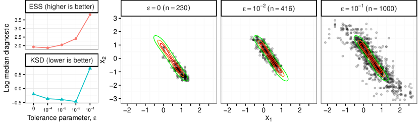
Figure 3: Left: Median hyperparameter selection criteria across $50$ independent approximate slice sampler sample sequences (see Section 4.3); IMQ KSD selects $\epsilon=10^{-2}$; effective sample size selects $\epsilon=10^{-1}$. Right: Representative approximate slice sampler samples requiring $148000$ likelihood evaluations with posterior equidensity contours overlaid; $n$ is the associated sample size.

4.4 Selecting samplers

Ahn et al. (2012) developed two biased MCMC samplers for accelerated posterior inference, both called Stochastic Gradient Fisher Scoring (SGFS). In the full version of SGFS (termed SGFS-f), a $d\times d$ matrix must be inverted to draw each new sample point. Since this can be costly for large $d$, the authors developed a second sampler (termed SGFS-d) in which only a diagonal matrix must be inverted to draw each new sample point. Both samplers can be viewed as discrete-time approximations to a continuous-time Markov process that has the target $P$ as its stationary distribution; however, because no Metropolis-Hastings correction is employed, neither sampler has the target as its stationary distribution. Hence we will use the KSD – a quality measure that accounts for asymptotic bias – to evaluate and choose between these samplers.

Specifically, we evaluate the SGFS-f and SGFS-d samples produced in (Ahn et al., 2012, Sec. 5.1). The target $P$ is a Bayesian logistic regression with a flat prior, conditioned on a dataset of $10^{4}$ MNIST handwritten digit images. From each image, the authors extracted $50$ random projections of the raw pixel values as covariates and a label indicating whether the image was a $7$ or a $9$. After discarding the first half of sample points as burn-in, we obtained regression coefficient samples with $5\times 10^{4}$ points and $d=51$ dimensions (including the intercept term). Figure 4 displays the IMQ KSD applied to the first $n$ points in each sample. As external validation, we follow the protocol of Ahn et al. (2012) to find the bivariate marginal means and 95% confidence ellipses of each sample that align best and worst with those of a surrogate ground truth sample obtained from a Hamiltonian Monte Carlo chain with $10^{5}$ iterates. Both the KSD and the surrogate ground truth suggest that the moderate speed-up provided by SGFS-d ($0.0017s$ per sample vs. $0.0019s$ for SGFS-f) is outweighed by the significant loss in inferential accuracy. However, the KSD assessment does not require access to an external trustworthy ground truth sample. The longest KSD computation took $400s$ using $16$ cores.

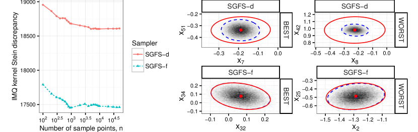
Figure 4: Left: Quality comparison for Bayesian logistic regression with two SGFS samplers (see Section 4.4). Right: Scatter plots of $n=5\times 10^{4}$ SGFS sample points with overlaid bivariate marginal means and 95% confidence ellipses (dashed blue) that align best and worst with surrogate ground truth sample (solid red).

4.5 Beyond sample quality comparison

While our investigation of the KSD was motivated by the desire to develop practical, trustworthy tools for sample quality comparison, the kernels recommended by our theory can serve as drop-in replacements in other inferential tasks that make use of kernel Stein discrepancies.

4.5.1 One-sample hypothesis testing

Chwialkowski et al. (2016) recently used the KSD $\mathcal{S}({Q_{n}},{\mathcal{T}_{P}{}},{\mathcal{G}_{k}})$ to develop a hypothesis test of whether a given sample from a Markov chain was drawn from a target distribution $P$ (see also Liu et al., 2016). However, the authors noted that the KSD test with their default Gaussian base kernel $k$ experienced a considerable loss of power as the dimension $d$ increased. We recreate their experiment and show that this loss of power can be avoided by using our default IMQ kernel with $\beta=-\frac{1}{2}$ and $c=1$. Following (Chwialkowski et al., 2016, Section 4) we draw $z_{i}\stackrel{{\scriptstyle\mathrm{iid}}}{{\sim}}\mathcal{N}(0,I_{d})$ and $u_{i}\stackrel{{\scriptstyle\mathrm{iid}}}{{\sim}}\textnormal{Unif}[0,1]$ to generate a sample $(x_{i})_{i=1}^{n}$ with $x_{i}=z_{i}+u_{i}\,e_{1}$ for $n=500$ and various dimensions $d$. Using the authors’ code (modified to include an IMQ kernel), we compare the power of the Gaussian KSD test, the IMQ KSD test, and the standard normality test of Baringhaus & Henze (1988) (B&H) to discern whether the sample $(x_{i})_{i=1}^{500}$ came from the null distribution $P=\mathcal{N}(0,I_{d})$. The results, averaged over $400$ simulations, are shown in Table 1. Notably, the IMQ KSD experiences no power degradation over this range of dimensions, thus improving on both the Gaussian KSD and the standard B&H normality tests.

Table 1: Power of one sample tests for multivariate normality, averaged over $400$ simulations (see Section 4.5.1)

	d=2	d=5	d=10	d=15	d=20	d=25
B&H	1.0	1.0	1.0	0.91	0.57	0.26
Gaussian	1.0	1.0	0.88	0.29	0.12	0.02
IMQ	1.0	1.0	1.0	1.0	1.0	1.0

4.5.2 Improving sample quality

Liu & Lee (2016) recently used the KSD $\mathcal{S}({Q_{n}},{\mathcal{T}_{P}{}},{\mathcal{G}_{k}})$ as a means of improving the quality of a sample. Specifically, given an initial sample $Q_{n}$ supported on $x_{1},\dots,x_{n}$, they minimize $\mathcal{S}({\tilde{Q}_{n}},{\mathcal{T}_{P}{}},{\mathcal{G}_{k}})$ over all measures $\tilde{Q}_{n}$ supported on the same sample points to obtain a new sample that better approximates $P$ over the class of test functions $\mathcal{H}=\mathcal{T}_{P}{\mathcal{G}_{k}}$. In all experiments, Liu & Lee (2016) employ a Gaussian kernel $k(x,y)=e^{-\frac{1}{h}\mathopen{}\mathclose{{}\left\|{x-y}}\right\|_{2}^{2}}$ with bandwidth $h$ selected to be the median of the squared Euclidean distance between pairs of sample points. Using the authors’ code, we recreate the experiment from (Liu & Lee, 2016, Fig. 2b) and introduce a KSD objective with an IMQ kernel $k(x,y)=(1+\frac{1}{h}\mathopen{}\mathclose{{}\left\|{x-y}}\right\|_{2}^{2})^{-1/2}$ with bandwidth selected in the same fashion. The starting sample is given by $Q_{n}=\frac{1}{n}\sum_{i=1}^{n}\delta_{x_{i}}$ for $n=100$, various dimensions $d$, and each sample point drawn i.i.d. from $P=\mathcal{N}(0,I_{d})$. For the initial sample and the optimized samples produced by each KSD, Figure 5 displays the mean squared error (MSE) $\frac{1}{d}\|{\mathbb{E}_{P}\mathopen{}\mathclose{{}\left[{{Z}}}\right]-\mathbb{E}_{\tilde{Q}_{n}}\mathopen{}\mathclose{{}\left[{X}}\right]}\|_{2}^{2}$ averaged across $500$ independently generated initial samples. Out of the box, the IMQ kernel produces better mean estimates than the standard Gaussian.

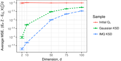
Figure 5: Average quality of mean estimates ($\pm 2$ standard errors) under optimized samples $\tilde{Q}_{n}$ for target $P=\mathcal{N}(0,I_{d})$; MSE averaged over $500$ independent initial samples (see Section 4.5.2).

5 Related and future work

The score statistic of Fan et al. (2006) and the Gibbs sampler convergence criteria of Zellner & Min (1995) detect certain forms of non-convergence but fail to detect others due to the finite number of test functions tested. For example, when $P=\mathcal{N}(0,1)$, the score statistic (Fan et al., 2006) only monitors sample means and variances.

For an approximation $\mu$ with continuously differentiable density $r$, Chwialkowski et al. (2016, Thm. 2.2) and Liu et al. (2016, Prop. 3.3) established that if $k$ is $C_{0}$-universal (Carmeli et al., 2010, Defn. 4.1) or integrally strictly positive definite (ISPD, Stewart, 1976, Sec. 6) and $\mathbb{E}_{\mu}[k_{0}(X,X)+\|{\nabla\log\frac{p(X)}{r(X)}}\|_{2}^{2}]<\infty$ for $k_{0}\triangleq\sum_{j=1}^{d}k_{0}^{j}$, then $\mathcal{S}({\mu},{\mathcal{T}_{P}{}},{\mathcal{G}_{k}})=0$ only if $\mu=P$. However, this property is insufficient to conclude that probability measures with small KSD are close to $P$ in any traditional sense. Indeed, Gaussian and Matérn kernels are $C_{0}$ universal and ISPD, but, by Theorem 6, their KSDs can be driven to zero by sequences not converging to $P$. On compact domains, where tightness is no longer an issue, the combined results of (Oates et al., 2016a, Lem. 4), (Fukumizu et al., 2007, Lem. 1), and (Simon-Gabriel & Schölkopf, 2016, Thm. 55) give conditions for a KSD to dominate weak convergence.

While assessing sample quality was our chief objective, our results may hold benefits for other applications that make use of Stein discrepancies or Stein operators. In particular, our kernel recommendations could be incorporated into the Monte Carlo control functionals framework of Oates et al. (2016b); Oates & Girolami (2015), the variational inference approaches of Liu & Wang (2016); Liu & Feng (2016); Ranganath et al. (2016), and the Stein generative adversarial network approach of Wang & Liu (2016).

In the future, we aim to leverage stochastic, low-rank, and sparse approximations of the kernel matrix and score function to produce KSDs that scale better with the number of sample and data points while still guaranteeing control over weak convergence. A reader may also wonder for which distributions outside of $\mathcal{P}$ the KSD dominates weak convergence. The following theorem, proved in Section J, shows that no KSD with a $C_{0}$ kernel dominates weak convergence when the target has a bounded score function.

Theorem 10 (KSD fails for bounded scores).

If $\nabla\log p$ is bounded and $k\in C^{(1,1)}_{0}$, then $\mathcal{S}({Q_{n}},{\mathcal{T}_{P}{}},{\mathcal{G}_{k}})\to 0$ does not imply $Q_{n}\Rightarrow P$.

However, Gorham et al. (2016) developed convergence-determining graph Stein discrepancies for heavy-tailed targets by replacing the Langevin Stein operator $\mathcal{T}_{P}{}$ with diffusion Stein operators of the form $(\mathcal{T}{g})({x})={\textstyle\frac{1}{p(x)}}\langle{\nabla},{p(x)(a(x)+c(x))g(x)}\rangle$. An analogous construction should yield convergence-determining diffusion KSDs for $P$ outside of $\mathcal{P}$. Our results also extend to targets $P$ supported on a convex subset $\mathcal{X}$ of $\mathbb{R}^{d}$ by choosing $k$ to satisfy $p(x)k(x,\cdot)\equiv 0$ for all $x$ on the boundary of $\mathcal{X}$.

Appendix A Additional appendix notation

We use $f\ast h$ to denote the convolution between $f$ and $h$, and, for absolutely integrable $f:\mathbb{R}^{d}\to\mathbb{R}$, we say $\hat{f}(\omega)\triangleq(2\pi)^{-d/2}\int f(x)e^{-i\langle{x},{\omega}\rangle}dx$ is the Fourier transform of $f$. For $g\in\mathcal{K}_{k}^{d}$ we define $\mathopen{}\mathclose{{}\left\|{g}}\right\|_{\mathcal{K}_{k}^{d}}\triangleq\sqrt{\sum_{j=1}^{d}\mathopen{}\mathclose{{}\left\|{g_{j}}}\right\|_{\mathcal{K}_{k}}^{2}}$. Let $L^{2}$ denote the Banach space of real-valued functions $f$ with $\mathopen{}\mathclose{{}\left\|{f}}\right\|_{L^{2}}\triangleq\int f(x)^{2}\,dx<\infty$. For $\mathbb{R}^{d}$-valued $g$, we will overload $g\in L^{2}$ to mean $\mathopen{}\mathclose{{}\left\|{g}}\right\|_{L^{2}}\triangleq\sqrt{\sum_{j=1}^{d}\mathopen{}\mathclose{{}\left\|{g_{j}}}\right\|_{L^{2}}^{2}}<\infty$. We define the operator norm of a vector $a\in\mathbb{R}^{d}$ as $\mathopen{}\mathclose{{}\left\|{a}}\right\|_{op}\triangleq\mathopen{}\mathclose{{}\left\|{a}}\right\|_{2}$ and of a matrix $A\in\mathbb{R}^{d\times d}$ as $\mathopen{}\mathclose{{}\left\|{A}}\right\|_{op}\triangleq\sup_{x\in\mathbb{R}^{d},\mathopen{}\mathclose{{}\left\|{x}}\right\|_{2}=1}\mathopen{}\mathclose{{}\left\|{Ax}}\right\|_{2}$. We further define the Lipschitz constant $M_{2}(g)\triangleq\sup_{x\neq y}\mathopen{}\mathclose{{}\left\|{\nabla g(x)-\nabla g(y)}}\right\|_{op}/\mathopen{}\mathclose{{}\left\|{x-y}}\right\|_{2}$ and the ball $\mathcal{B}(x,r)\triangleq\{y\in\mathbb{R}^{d}\,|\,\mathopen{}\mathclose{{}\left\|{x-y}}\right\|_{2}\leq r\}$ for any $x\in\mathbb{R}^{d}$ and $r\geq 0$.

Appendix B Proof of Proposition 1: Zero mean test functions

Fix any $g\in\mathcal{G}$. Since $k\in C^{(1,1)}$, $\sup_{x\in\mathbb{R}^{d}}k(x,x)<\infty$, and $\sup_{x\in\mathbb{R}^{d}}\mathopen{}\mathclose{{}\left\|{\nabla_{x}\nabla_{y}k(x,x)}}\right\|_{op}<\infty$, Cor. 4.36 of (Steinwart & Christmann, 2008) implies that $M_{0}(g_{j})<\infty$ and $M_{1}(g_{j})<\infty$ for each $j\in\{1,\dots,d\}$. As $\mathbb{E}_{P}\mathopen{}\mathclose{{}\left[{\mathopen{}\mathclose{{}\left\|{b(Z)}}\right\|_{2}}}\right]<\infty$, the proof of (Gorham & Mackey, 2015, Prop. 1) now implies $\mathbb{E}_{P}\mathopen{}\mathclose{{}\left[{(\mathcal{T}_{P}{g})({Z})}}\right]=0$.

Appendix C Proof of Proposition 2: KSD closed form

Our proof generalizes that of (Chwialkowski et al., 2016, Thm. 2.1). For each dimension $j\in\{1,\dots,d\}$, we define the operator $\mathcal{T}_{P}^{j}{}$ via $(\mathcal{T}_{P}^{j}{g_{0}})(x)\triangleq\frac{1}{p(x)}\nabla_{x_{j}}(p(x)g_{0}(x))=\nabla_{x_{j}}g_{0}(x)+b_{j}(x)g_{0}(x)$ for $g_{0}:\mathbb{R}^{d}\to\mathbb{R}$. We further let $\Psi_{k}:\mathbb{R}^{d}\to\mathcal{K}_{k}$ denote the canonical feature map of $\mathcal{K}_{k}$, given by $\Psi_{k}(x)\triangleq k(x,\cdot)$. Since $k\in C^{(1,1)}$, the argument of (Steinwart & Christmann, 2008, Cor. 4.36) implies that

$$\mathcal{T}_{P}{g}(x) \textstyle=\sum_{j=1}^{d}(\mathcal{T}_{P}^{j}{g_{j}})(x)=\sum_{j=1}^{d}\mathcal{T}_{P}^{j}{\langle{g_{j}},{\Psi_{k}(x)}\rangle_{\mathcal{K}_{k}}}=\sum_{j=1}^{d}\langle{g_{j}},{\mathcal{T}_{P}^{j}{}\Psi_{k}(x)}\rangle_{\mathcal{K}_{k}}$$ (5)

for all $g=(g_{1},\dots,g_{d})\in\mathcal{G}_{k,\mathopen{}\mathclose{{}\left\|{\cdot}}\right\|}$ and $x\in\mathbb{R}^{d}$. Moreover, (Steinwart & Christmann, 2008, Lem. 4.34) gives

$$\langle{\mathcal{T}_{P}^{j}{\Psi}_{k}(x)},{\mathcal{T}_{P}^{j}{\Psi}_{k}(y)}\rangle =\langle b_{j}(x)\Psi_{k}(x)+\nabla_{x_{j}}\Psi_{k}(x),b_{j}(y)\Psi_{k}(y)+\nabla_{y_{j}}\Psi_{k}(y)\rangle_{\mathcal{K}_{k}}$$

$$=b_{j}(x)b_{j}(y)k(x,y)+b_{j}(x)\nabla_{y_{j}}k(x,y)+b_{j}(y)\nabla_{x_{j}}k(x,y)+\nabla_{x_{j}}\nabla_{y_{j}}k(x,y)=k_{0}^{j}(x,y)$$ (6)

for all $x,y\in\mathbb{R}^{d}$ and $j\in\{1,\dots,d\}$. The representation (C) and our $\mu$-integrability assumption together imply that, for each $j$, $\mathcal{T}_{P}^{j}{\Psi_{k}}$ is Bochner $\mu$-integrable (Steinwart & Christmann, 2008, Definition A.5.20), since

$$\mathbb{E}_{\mu}\mathopen{}\mathclose{{}\left[{\mathopen{}\mathclose{{}\left\|{\mathcal{T}_{P}^{j}{\Psi_{k}(X)}}}\right\|_{\mathcal{K}_{k}}}}\right]=\mathbb{E}_{\mu}\mathopen{}\mathclose{{}\left[{\sqrt{k_{0}^{j}(X,X)}}}\right]<\infty.$$

Hence, we may apply the representation (C) and exchange expectation and RKHS inner product to discover

$$w_{j}^{2}=\mathbb{E}\mathopen{}\mathclose{{}\left[{k_{0}^{j}(X,\tilde{X})}}\right]=\mathbb{E}\mathopen{}\mathclose{{}\left[{\langle{\mathcal{T}_{P}^{j}{\Psi_{k}(X)}},{\mathcal{T}_{P}^{j}{\Psi_{k}(\tilde{X})}}\rangle_{\mathcal{K}_{k}}}}\right]=\mathopen{}\mathclose{{}\left\|{\mathbb{E}_{\mu}\mathopen{}\mathclose{{}\left[{\mathcal{T}_{P}^{j}{\Psi_{k}({X})}}}\right]}}\right\|_{\mathcal{K}_{k}}^{2}.$$ (7)

for $X,\tilde{X}\stackrel{{\scriptstyle\mathrm{iid}}}{{\sim}}\mu$. To conclude, we invoke the representation (5), Bochner $\mu$-integrability, the representation (7), and the Fenchel-Young inequality for dual norms twice:

$$\mathcal{S}({\mu},{\mathcal{T}_{P}{}},{\mathcal{G}_{k,\mathopen{}\mathclose{{}\left\|{\cdot}}\right\|}}) =\sup_{g\in\mathcal{G}_{k,\mathopen{}\mathclose{{}\left\|{\cdot}}\right\|}}\mathbb{E}_{\mu}[(\mathcal{T}_{P}{g})({{X}})]=\sup_{\mathopen{}\mathclose{{}\left\|{g_{j}}}\right\|_{\mathcal{K}_{k}}=v_{j},\mathopen{}\mathclose{{}\left\|{v}}\right\|^{*}\leq 1}{\textstyle\sum}_{j=1}^{d}\langle{g_{j}},{\mathbb{E}_{\mu}[\mathcal{T}_{P}^{j}{\Psi_{k}({X})}]}\rangle_{\mathcal{K}_{k}}$$

$$=\sup_{\mathopen{}\mathclose{{}\left\|{v}}\right\|^{*}\leq 1}{\textstyle\sum}_{j=1}^{d}v_{j}\mathopen{}\mathclose{{}\left\|{\mathbb{E}_{\mu}[\mathcal{T}_{P}^{j}{\Psi_{k}({X})}]}}\right\|_{\mathcal{K}_{k}}=\sup_{\mathopen{}\mathclose{{}\left\|{v}}\right\|^{*}\leq 1}{\textstyle\sum}_{j=1}^{d}v_{j}w_{j}=\mathopen{}\mathclose{{}\left\|{w}}\right\|.$$

Appendix D Proof of Proposition 3: Stein set equivalence

By Proposition 2, $\mathcal{S}({\mu},{\mathcal{T}_{P}{}},{\mathcal{G}_{k,\mathopen{}\mathclose{{}\left\|{\cdot}}\right\|}})=\mathopen{}\mathclose{{}\left\|{w}}\right\|$ and $\mathcal{S}({\mu},{\mathcal{T}_{P}{}},{\mathcal{G}_{k,\mathopen{}\mathclose{{}\left\|{\cdot}}\right\|_{2}}})=\mathopen{}\mathclose{{}\left\|{w}}\right\|_{2}$ for some vector $w$, and by (Bachman & Narici, 1966, Thm. 8.7), there exist constants $c_{d},c_{d}^{\prime}>0$ depending only on $d$ and $\mathopen{}\mathclose{{}\left\|{\cdot}}\right\|$ such that $c_{d}\mathopen{}\mathclose{{}\left\|{w}}\right\|\leq\mathopen{}\mathclose{{}\left\|{w}}\right\|_{2}\leq c_{d}^{\prime}\mathopen{}\mathclose{{}\left\|{w}}\right\|$.

Appendix E Proof of Theorem 5: Univariate KSD detects non-convergence

While the statement of Theorem 5 applies only to the univariate case $d=1$, we will prove all steps for general $d$ when possible. Our strategy is to define a reference IPM $d_{\mathcal{H}}$ for which $\mu_{m}\Rightarrow P$ whenever $d_{\mathcal{H}}(\mu_{m},P)\to 0$ and then upper bound $d_{\mathcal{H}}$ by a function of the KSD $\mathcal{S}({\mu_{m}},{\mathcal{T}_{P}{}},{\mathcal{G}_{k}})$. To construct the reference class of test functions $\mathcal{H}$, we choose some integrally strictly positive definite (ISPD) kernel $k_{b}:\mathbb{R}^{d}\times\mathbb{R}^{d}\to\mathbb{R}$, that is, we select a kernel function $k_{b}$ such that

$$\int_{\mathbb{R}^{d}\times\mathbb{R}^{d}}k_{b}(x,y)d\mu(x)d\mu(y)>0$$

for all finite non-zero signed Borel measures $\mu$ on $\mathbb{R}^{d}$ (Sriperumbudur et al., 2010, Section 1.2). For this proof, we will choose the Gaussian kernel $k_{b}(x,y)=\operatorname{exp}\mathopen{}\mathclose{{}\left(-\mathopen{}\mathclose{{}\left\|{x-y}}\right\|_{2}^{2}/2}\right)$, which is ISPD by (Sriperumbudur et al., 2010, Section 3.1). Since $r(x)\triangleq\operatorname{exp}\mathopen{}\mathclose{{}\left(-\mathopen{}\mathclose{{}\left\|{x}}\right\|_{2}^{2}/2}\right)$ is bounded and continuous and never vanishes, the kernel $\tilde{k_{b}}(x,y)=k_{b}(x,y)r(x)r(y)$ is also ISPD. Let $\mathcal{H}\triangleq\{h\in\mathcal{K}_{\tilde{k_{b}}}\,|\,\mathopen{}\mathclose{{}\left\|{h}}\right\|_{\tilde{k_{b}}}\leq 1\}$. By (Sriperumbudur, 2016, Thm. 3.2), since $\tilde{k_{b}}$ is ISPD with $\tilde{k_{b}}(x,\cdot)\in C_{0}(\mathbb{R}^{d})$ for all $x$, we know that $d_{\mathcal{H}}(\mu_{m},P)\to 0$ only if $\mu_{m}\Rightarrow P$. With $\mathcal{H}$ in hand, Theorem 5 will follow from our next theorem which upper bounds the IPM $d_{\mathcal{H}}(\mu,P)$ in terms of the KSD $\mathcal{S}({\mu},{\mathcal{T}_{P}{}},{\mathcal{G}_{k}})$.

Theorem 11 (Univariate KSD lower bound).

Let $d=1$, and consider the set of univariate functions $\mathcal{H}=\{h\in\mathcal{K}_{\tilde{k_{b}}}\,|\,\mathopen{}\mathclose{{}\left\|{h}}\right\|_{\tilde{k_{b}}}\leq 1\}$. Suppose $P\in\mathcal{P}$ and $k(x,y)=\Phi(x-y)$ for $\Phi\in C^{2}$ with generalized Fourier transform $\hat{\Phi}$ and $F(t)\triangleq\sup_{\mathopen{}\mathclose{{}\left\|{\omega}}\right\|_{\infty}\leq t}\hat{\Phi}(\omega)^{-1}$ finite for all $t>0$. Then there exists a constant $\mathcal{M}_{P}>0$ such that, for all probability measures $\mu$ and $\epsilon>0$,

$$\textstyle d_{\mathcal{H}}(\mu,P)\leq\epsilon+\mathopen{}\mathclose{{}\left(\frac{\pi}{2}}\right)^{1/4}\mathcal{M}_{P}F\mathopen{}\mathclose{{}\left(\frac{12\log 2}{\pi}(1+\sqrt{d-1}+M_{1}(b)\mathcal{M}_{P})\epsilon^{-1}}\right)^{1/2}\mathcal{S}({\mu},{\mathcal{T}_{P}{}},{\mathcal{G}_{k}}).$$

Remarks     An explicit value for the Stein factor $\mathcal{M}_{P}$ can be derived from the proof in Section E.1 and the results of Gorham et al. (2016). After optimizing the bound $d_{\mathcal{H}}(\mu,P)$ over $\epsilon>0$, the Gaussian, inverse multiquadric, and Matérn ($v>1$) kernels achieve rates of $O(1/\sqrt{\log(\frac{1}{\mathcal{S}({\mu},{\mathcal{T}_{P}{}},{\mathcal{G}_{k}})})})$, $O(1/\log(\frac{1}{\mathcal{S}({\mu},{\mathcal{T}_{P}{}},{\mathcal{G}_{k}})}))$, and $O(\mathcal{S}({\mu},{\mathcal{T}_{P}{}},{\mathcal{G}_{k}})^{1/(v+1/2)})$ respectively as $\mathcal{S}({\mu},{\mathcal{T}_{P}{}},{\mathcal{G}_{k}})\to 0$.

In particular, since $\hat{\Phi}$ is non-vanishing, $F(t)$ is finite for all $t$. If $\mathcal{S}({\mu_{m}},{\mathcal{T}_{P}{}},{\mathcal{G}_{k}})\to 0$, then, for any fixed $\epsilon>0$, we have $\lim\sup_{m\to\infty}d_{\mathcal{H}}(\mu_{m},P)\leq\epsilon$. Taking $\epsilon\to 0$ shows that $\lim_{m\to\infty}d_{\mathcal{H}}(\mu_{m},P)\to 0$, which implies that $\mu_{m}\Rightarrow P$.

E.1 Proof of Theorem 11: Univariate KSD lower bound

Fix any probability measure $\mu$ and $h\in\mathcal{H}$, and define the tilting function $\Xi(x)\triangleq(1+\mathopen{}\mathclose{{}\left\|{x}}\right\|_{2}^{2})^{1/2}$. The proof will proceed in three steps.

Step 1: Uniform bounds on $M_{0}(h)$, $M_{1}(h)$ and $\sup_{x\in\mathbb{R}^{d}}\mathopen{}\mathclose{{}\left\|{\Xi(x)\nabla h(x)}}\right\|_{2}$

We first bound $M_{0}(h)$, $M_{1}(h)$ and $\sup_{x\in\mathbb{R}^{d}}\mathopen{}\mathclose{{}\left\|{\Xi(x)\nabla h(x)}}\right\|_{2}$ uniformly over $\mathcal{H}$. To this end, we define the finite value $c_{0}\triangleq\sup_{x\in\mathbb{R}^{d}}(1+\mathopen{}\mathclose{{}\left\|{x}}\right\|_{2}^{2})r(x)=2e^{-1/2}$. For all $x\in\mathbb{R}^{d}$, we have

$$|h(x)|=|\langle{h},{\tilde{k_{b}}(x,\cdot)}\rangle_{\mathcal{K}_{\tilde{k_{b}}}}|\leq\mathopen{}\mathclose{{}\left\|{h}}\right\|_{\mathcal{K}_{\tilde{k_{b}}}}\,\tilde{k_{b}}(x,x)^{1/2}\leq 1.$$

Moreover, we have $\nabla_{x}k_{b}(x,y)=(y-x)k_{b}(x,y)$ and $\nabla r(x)=-xr(x)$. Thus for any $x$, by (Steinwart & Christmann, 2008, Corollary 4.36) we have

$$\mathopen{}\mathclose{{}\left\|{\nabla h(x)}}\right\|_{2}\leq\mathopen{}\mathclose{{}\left\|{h}}\right\|_{\mathcal{K}_{\tilde{k_{b}}}}\,\langle{\nabla_{x}},{\nabla_{y}\tilde{k_{b}}(x,x)}\rangle^{1/2}\leq[d\,r(x)^{2}+\mathopen{}\mathclose{{}\left\|{x}}\right\|_{2}^{2}\,r(x)^{2}]^{1/2}k_{b}(x,x)^{1/2}\leq[(d-1)^{1/2}+(1+\mathopen{}\mathclose{{}\left\|{x}}\right\|_{2}^{2})^{1/2})]r(x),$$

where in the last inequality we used the triangle inequality. Hence $\mathopen{}\mathclose{{}\left\|{\nabla h(x)}}\right\|_{2}\leq(d-1)^{1/2}+1$ and $\mathopen{}\mathclose{{}\left\|{\Xi(x)\nabla h(x)}}\right\|_{2}\leq(d-1)^{1/2}+c_{0}$ for all $x$, completing our bounding of $M_{0}(h)$, $M_{1}(h)$ and $\sup_{x\in\mathbb{R}^{d}}\mathopen{}\mathclose{{}\left\|{\Xi(x)\nabla h(x)}}\right\|_{2}$ uniformly over $\mathcal{H}$.

Step 2: Uniform bound on $\mathopen{}\mathclose{{}\left\|{g_{h}}}\right\|_{L^{2}}$ for Stein solution $g_{h}$

We next show that there is a solution to the $P$ Stein equation

$$(\mathcal{T}_{P}{g_{h}})({x})=h(x)-\mathbb{E}_{P}\mathopen{}\mathclose{{}\left[{h(Z)}}\right]$$ (8)

with $g_{h}(x)\leq\mathcal{M}_{P}/(1+\mathopen{}\mathclose{{}\left\|{x}}\right\|_{2}^{2})^{1/2}$ for every $h\in\mathcal{H}$. When $d=1$, this will imply that $\mathopen{}\mathclose{{}\left\|{g_{h}}}\right\|_{L^{2}}$ is bounded uniformly over $\mathcal{H}$. To proceed, we will define a tilted distribution $\tilde{P}\in\mathcal{P}$ and a tilted function $f$, show that a solution $\tilde{g}_{f}$ to the $\tilde{P}$ Stein equation is bounded, and construct a solution $g_{h}$ to the Stein equation of $P$ based on $\tilde{g}_{f}$.

Define $\tilde{P}$ via the tilted probability density $\tilde{p}(x)\propto p(x)/\Xi(x)$ with score function $\tilde{b}(x)\triangleq\nabla\log\tilde{p}(x)=b(x)-\xi(x)$ for $\xi(x)\triangleq\nabla\log\Xi(x)=x/(1+\mathopen{}\mathclose{{}\left\|{x}}\right\|_{2}^{2})$. Since $b$ is Lipschitz and $\nabla\xi(x)=(1+\mathopen{}\mathclose{{}\left\|{x}}\right\|_{2}^{2})^{-1}[I-2\frac{xx^{\top}}{1+\mathopen{}\mathclose{{}\left\|{x}}\right\|_{2}^{2}}]$ has its operator norm uniformly bounded by $3$, $\tilde{b}$ is also Lipschitz. To see that $\tilde{P}$ is also distantly dissipative, note first that $|\langle{\xi(x)-\xi(y)},{x-y}\rangle|\leq\mathopen{}\mathclose{{}\left\|{\xi(x)-\xi(y)}}\right\|_{2}\cdot\mathopen{}\mathclose{{}\left\|{x-y}}\right\|_{2}\leq\mathopen{}\mathclose{{}\left\|{x-y}}\right\|_{2}$ since $\sup_{x}\mathopen{}\mathclose{{}\left\|{\xi(x)}}\right\|_{2}\leq 1/2$. Because $P$ is distantly dissipative, we know $\langle{b(x)-b(y)},{x-y}\rangle\leq-\frac{1}{2}\kappa_{0}\mathopen{}\mathclose{{}\left\|{x-y}}\right\|_{2}^{2}$ for some $\kappa_{0}>0$ and all $\mathopen{}\mathclose{{}\left\|{x-y}}\right\|_{2}\geq R$ for some $R>0$. Thus for all $\mathopen{}\mathclose{{}\left\|{x-y}}\right\|_{2}\geq\max(R,4/\kappa_{0})$, we have

$$\langle{\tilde{b}(x)-\tilde{b}(y)},{x-y}\rangle=\langle{b(x)-b(y)},{x-y}\rangle+\langle{\xi(x)-\xi(y)},{x-y}\rangle\leq-\frac{1}{2}\kappa_{0}\mathopen{}\mathclose{{}\left\|{x-y}}\right\|_{2}^{2}+\mathopen{}\mathclose{{}\left\|{x-y}}\right\|_{2}\leq-\frac{1}{2}\frac{\kappa_{0}}{2}\mathopen{}\mathclose{{}\left\|{x-y}}\right\|_{2}^{2},$$

so $\tilde{P}$ is also distantly dissipative and hence in $\mathcal{P}$.

Let $f(x)\triangleq\Xi(x)(h(x)-\mathbb{E}_{P}\mathopen{}\mathclose{{}\left[{h(Z)}}\right])$. Since $\mathbb{E}_{\tilde{P}}\mathopen{}\mathclose{{}\left[{f(Z)}}\right]=\mathbb{E}_{P}\mathopen{}\mathclose{{}\left[{h(Z)-\mathbb{E}_{P}\mathopen{}\mathclose{{}\left[{h(Z)}}\right]}}\right]=0$, Thm. 5 and Sec. 4.2 of (Gorham et al., 2016), imply that the $\tilde{P}$ Stein equation $(\mathcal{T}_{\tilde{P}}{\tilde{g}_{f}})(x)=f(x)$ has a solution $\tilde{g}_{f}$ with $M_{0}(g_{f})\leq\mathcal{M}_{P}^{\prime}M_{1}(f)$ for $\mathcal{M}_{P}^{\prime}$ a constant independent of $f$ and $h$. Since $\nabla f(x)=\nabla\Xi(x)(h(x)-\mathbb{E}_{P}\mathopen{}\mathclose{{}\left[{h(Z)}}\right])+\Xi(x)\nabla h(x)$ and $\mathopen{}\mathclose{{}\left\|{\nabla\Xi(x)}}\right\|_{2}=\frac{\mathopen{}\mathclose{{}\left\|{x}}\right\|_{2}}{(1+\mathopen{}\mathclose{{}\left\|{x}}\right\|_{2}^{2})^{1/2}}$ is bounded by $1$, $M_{0}(g_{f})\leq\mathcal{M}_{P}^{\prime}(2+(d-1)^{1/2}+c_{0})\triangleq\mathcal{M}_{P}$, a constant independent of $h$.

Finally, we note that $g_{h}(x)\triangleq\tilde{g}_{f}(x)/\Xi(x)$ is a solution to the $P$ Stein equation (8) satisfying $g_{h}(x)\leq\mathcal{M}_{P}/\Xi(x)=\mathcal{M}_{P}/(1+\mathopen{}\mathclose{{}\left\|{x}}\right\|_{2}^{2})^{1/2}$. Hence, in the case $d=1$, we have $\mathopen{}\mathclose{{}\left\|{g_{h}}}\right\|_{L^{2}}\leq\mathcal{M}_{P}\sqrt{\pi}$.

Step 3: Approximate $\mathcal{T}_{P}{g_{h}}$ using $\mathcal{T}_{P}{\mathcal{G}_{k}}$

In our final step, we will use the following lemma, proved in Section E.2, to show that we can approximate $\mathcal{T}_{P}{g_{h}}$ arbitrarily well by a function in a scaled copy of $\mathcal{T}_{P}{\mathcal{G}_{k}}$.

Lemma 12 (Stein approximations with finite RKHS norm).

Suppose that $g:\mathbb{R}^{d}\to\mathbb{R}^{d}$ is bounded and belongs to $L^{2}\cap C^{1}$ and that $h=\mathcal{T}_{P}{g}$ and $\nabla\log p$ are Lipschitz. Moreover, suppose $k(x,y)=\Phi(x-y)$ for $\Phi\in C^{2}$ with generalized Fourier transform $\hat{\Phi}$. Then for every $\epsilon>0$, there is a function $g_{\epsilon}:\mathbb{R}^{d}\to\mathbb{R}^{d}$ such that $\sup_{x\in\mathbb{R}^{d}}|(\mathcal{T}_{P}{g_{\epsilon}})({x})-(\mathcal{T}_{P}{g})({x})|\leq\epsilon$ and

$$\textstyle\mathopen{}\mathclose{{}\left\|{g_{\epsilon}}}\right\|_{\mathcal{K}_{k}^{d}}\leq(2\pi)^{-d/4}F\mathopen{}\mathclose{{}\left(\frac{12d\log 2}{\pi}(M_{1}(h)+M_{1}(b)M_{0}(g))\epsilon^{-1}}\right)^{1/2}\mathopen{}\mathclose{{}\left\|{g}}\right\|_{L^{2}},$$

where $F(t)\triangleq\sup_{\mathopen{}\mathclose{{}\left\|{\omega}}\right\|_{\infty}\leq t}\hat{\Phi}(\omega)^{-1}$.

When $d=1$, Lemma 12 implies that for every $\epsilon>0$ there is a function $g_{\epsilon}:\mathbb{R}\to\mathbb{R}$ such that $M_{0}(\mathcal{T}_{P}{g_{\epsilon}}-h)\leq\epsilon$ and $\mathopen{}\mathclose{{}\left\|{g_{\epsilon}}}\right\|_{\mathcal{K}_{k}}\leq(\frac{\pi}{2})^{1/4}\mathcal{M}_{P}F(\frac{12\log 2}{\pi}(M_{1}(h)+M_{1}(b)\mathcal{M}_{P})\epsilon^{-1})^{1/2}$. Hence we have

$$|\mathbb{E}_{P}\mathopen{}\mathclose{{}\left[{h({Z})}}\right]-\mathbb{E}_{\mu}\mathopen{}\mathclose{{}\left[{h({X})}}\right]| \leq|\mathbb{E}_{\mu}\mathopen{}\mathclose{{}\left[{h({X})-(\mathcal{T}_{P}{g_{\epsilon}})({{X}})}}\right]|+|\mathbb{E}_{\mu}\mathopen{}\mathclose{{}\left[{(\mathcal{T}_{P}{g_{\epsilon}})({{X}})}}\right]|$$

$$\leq\epsilon+\mathopen{}\mathclose{{}\left\|{g_{\epsilon}}}\right\|_{\mathcal{K}_{k}}\mathcal{S}({\mu},{\mathcal{T}_{P}{}},{\mathcal{G}_{k}})$$

$$\textstyle\leq\epsilon+(2\pi)^{-1/4}\mathcal{M}_{P}\sqrt{\pi}F\mathopen{}\mathclose{{}\left(\frac{12\log 2}{\pi}(M_{1}(h)+M_{1}(b)\mathcal{M}_{P})\epsilon^{-1}}\right)^{1/2}\mathcal{S}({\mu},{\mathcal{T}_{P}{}},{\mathcal{G}_{k}}).$$

Taking a supremum over $h\in\mathcal{H}$ yields the advertised result.

E.2 Proof of Lemma 12: Stein approximations with finite RKHS norm

Let us define the function $S:\mathbb{R}^{d}\to\mathbb{R}$ via the mapping $S(x)\triangleq\prod_{j=1}^{d}\frac{\sin x_{j}}{x_{j}}$. Then $S\in L^{2}$ and $\int_{\mathbb{R}^{d}}\mathopen{}\mathclose{{}\left\|{x}}\right\|_{2}S(x)^{4}<\infty$. We will then define the density function $\rho(x)\triangleq\mathcal{Z}^{-1}S(x)^{4}$, where $\mathcal{Z}\triangleq\int_{\mathbb{R}^{d}}S(x)^{4}\,dx=(2\pi/3)^{d}$ is the normalization constant. One can check that $\hat{\rho}(\omega)^{2}\leq(2\pi)^{-d}\mathbb{I}\mathopen{}\mathclose{{}\left[{\mathopen{}\mathclose{{}\left\|{\omega}}\right\|_{\infty}\leq 4}}\right]$.

Let $Y$ be a random variable with density $\rho$. For each $\delta>0$, let us define $\rho_{\delta}(x)=\delta^{-d}\rho(x/\delta)$ and for any function $f$ let us denote $f_{\delta}(x)\triangleq\mathbb{E}\mathopen{}\mathclose{{}\left[{f(x-\delta Y)}}\right]$. Since $h=\mathcal{T}_{P}{g}$ is assumed Lipschitz, this implies $|h_{\delta}(x)-h(x)|=|\mathbb{E}_{\rho}\mathopen{}\mathclose{{}\left[{h(x-\delta Y)-h(x)}}\right]|\leq\delta\,M_{1}(h)\,\mathbb{E}_{\rho}\mathopen{}\mathclose{{}\left[{\mathopen{}\mathclose{{}\left\|{Y}}\right\|_{2}}}\right]$ for all $x\in\mathbb{R}^{d}$.

Next, notice that for any $\delta>0$ and $x\in\mathbb{R}^{d}$,

$$(\mathcal{T}_{P}{g_{\delta}})({x}) =\mathbb{E}_{\rho}\mathopen{}\mathclose{{}\left[{\langle{b(x)},{g(x-\delta Y)}\rangle}}\right]+\mathbb{E}\mathopen{}\mathclose{{}\left[{\langle{\nabla},{g(x-\delta Y)}\rangle}}\right],\quad\text{and}\quad$$

$$h_{\delta}(x) =\mathbb{E}_{\rho}\mathopen{}\mathclose{{}\left[{\langle{b(x-\delta Y)},{g(x-\delta Y)}\rangle}}\right]+\mathbb{E}\mathopen{}\mathclose{{}\left[{\langle{\nabla},{g(x-\delta Y)}\rangle}}\right].$$

Because we assume $b$ is Lipschitz, we can deduce from above for any $x\in\mathbb{R}^{d}$,

$$|(\mathcal{T}_{P}{g_{\delta}})({x})-h_{\delta}(x)| =|\mathbb{E}_{\rho}\mathopen{}\mathclose{{}\left[{\langle{b(x)-b(x-\delta Y)},{g(x-\delta Y)}\rangle}}\right]|$$

$$\leq\mathbb{E}_{\rho}\mathopen{}\mathclose{{}\left[{\mathopen{}\mathclose{{}\left\|{b(x)-b(x-\delta Y)}}\right\|_{2}\mathopen{}\mathclose{{}\left\|{g(x-\delta Y)}}\right\|_{2}}}\right]$$

$$\leq M_{0}(g)\,M_{1}(b)\,\delta\,\mathbb{E}_{\rho}\mathopen{}\mathclose{{}\left[{\mathopen{}\mathclose{{}\left\|{Y}}\right\|_{2}}}\right].$$

Thus for any $\delta>0$, by the triangle inequality, we have

$$|(\mathcal{T}_{P}{g_{\delta}})({x})-(\mathcal{T}_{P}{g})({x})|\leq|(\mathcal{T}_{P}{g_{\delta}})({x})-h_{\delta}(x)|+|h_{\delta}(x)-h(x)|\leq\delta(M_{1}(h)+M_{1}(b)M_{0}(g))\mathbb{E}_{\rho}\mathopen{}\mathclose{{}\left[{\mathopen{}\mathclose{{}\left\|{Y}}\right\|_{2}}}\right].$$ (9)

Letting $\tilde{\epsilon}=\epsilon/((M_{1}(h)+M_{1}(b)M_{0}(g))\mathbb{E}_{\rho}\mathopen{}\mathclose{{}\left[{\mathopen{}\mathclose{{}\left\|{Y}}\right\|_{2}}}\right])$ for any $\epsilon>0$, we have $M_{0}(\mathcal{T}_{P}{g_{\tilde{\epsilon}}}-\mathcal{T}_{P}{g})\leq\epsilon$.

Thus it remains to bound the RKHS norm of $g_{\delta}$. By the Convolution Theorem (Wendland, 2004, Thm. 5.16), we have $\hat{g_{\delta}}(\omega)=(2\pi)^{d/2}\hat{g}(\omega)\hat{\rho_{\delta}}(\omega)$, and so the squared norm of $g_{\delta}$ in $\mathcal{K}_{k}^{d}$ is equal to (Wendland, 2004, Thm. 10.21)

$$(2\pi)^{-d/2}\int_{\mathbb{R}^{d}}\frac{|\hat{g_{\delta}}(\omega)|^{2}}{\hat{\Phi}(\omega)}\,d\omega=(2\pi)^{d/2}\int_{\mathbb{R}^{d}}\frac{|\hat{g}(\omega)|^{2}\hat{\rho_{\delta}}(\omega)^{2}}{\hat{\Phi}(\omega)}\,d\omega\leq(2\pi)^{-d/2}\mathopen{}\mathclose{{}\left\{\sup_{\mathopen{}\mathclose{{}\left\|{\omega}}\right\|_{\infty}\leq 4\delta^{-1}}\hat{\Phi}(\omega)^{-1}}\right\}\int_{\mathbb{R}^{d}}|\hat{g}(\omega)|^{2}\,d\omega,$$

where in the inequality we used the fact that $\hat{\rho_{\delta}}(\omega)=\hat{\rho}(\delta\omega)$. By Plancherel’s theorem (Herb & Sally Jr., 2011, Thm. 1.1), we know that $f\in L^{2}$ implies that $\mathopen{}\mathclose{{}\left\|{f}}\right\|_{L^{2}}=\|{\hat{f}}\|_{L^{2}}$. Thus we have $\mathopen{}\mathclose{{}\left\|{g_{\delta}}}\right\|_{\mathcal{K}_{k}^{d}}\leq(2\pi)^{-d/4}F(4\delta^{-1})^{1/2}\mathopen{}\mathclose{{}\left\|{g}}\right\|_{L^{2}}$. The final result follows from noticing that $\int_{\mathbb{R}}\sin^{4}(x)/x^{4}\,dx=\frac{2\pi}{3}$ and also

$$\int_{\mathbb{R}^{d}}\mathopen{}\mathclose{{}\left\|{x}}\right\|_{2}\prod_{j=1}^{d}\frac{\sin^{4}x_{j}}{x_{j}^{4}}\,dx\leq\int_{\mathbb{R}^{d}}\mathopen{}\mathclose{{}\left\|{x}}\right\|_{1}\prod_{j=1}^{d}\frac{\sin^{4}x_{j}}{x_{j}^{4}}\,dx=\sum_{j=1}^{d}\int_{\mathbb{R}^{d}}\frac{(\sin x_{j})^{4}}{|x_{j}|^{3}}\prod_{k\neq j}\frac{\sin^{4}x_{k}}{x_{k}^{4}}\,dx=2d(\log 2)\mathopen{}\mathclose{{}\left(\frac{2\pi}{3}}\right)^{d-1},$$

which implies $\mathbb{E}_{\rho}\mathopen{}\mathclose{{}\left[{\mathopen{}\mathclose{{}\left\|{Y}}\right\|_{2}}}\right]\leq\frac{3d\log 2}{\pi}$.

Appendix F Proof of Theorem 6: KSD fails with light kernel tails

First, define the generalized inverse function $\gamma^{-1}(s)\triangleq\inf\{r\geq 0\,|\,\gamma(r)\leq s\}$. Next, fix an $n\geq 1$, let $\Delta_{n}\triangleq\max(1,\gamma^{-1}(1/n))$, and define $r_{n}\triangleq\Delta_{n}n^{1/d}$. Select $n$ distinct points $x_{1},\dots,x_{n}\in\mathbb{R}^{d}$ so that $z_{i,i^{\prime}}\triangleq x_{i}-x_{i^{\prime}}$ satisfies $\mathopen{}\mathclose{{}\left\|{z_{i,i^{\prime}}}}\right\|_{2}>\Delta_{n}$ for all $i\neq i^{\prime}$ and $\mathopen{}\mathclose{{}\left\|{x_{i}}}\right\|_{2}\leq r_{n}$ for all $i$. By (Wainwright, 2017, Lems. 5.1 and 5.2), such a point set always exists. Now define $Q_{n}=\frac{1}{n}\sum_{i=1}^{n}\delta_{x_{i}}$. We will show that if $\Delta_{n}$ grows at an appropriate rate then $\mathcal{S}({Q_{n}},{\mathcal{T}_{P}{}},{\mathcal{G}_{k}})\to 0$ as $n\to\infty$.

Since the target distribution $P$ is $\mathcal{N}(0,I_{d})$, the associated gradient of the log density is $b(x)=-x$. Thus

$$k_{0}(x,y)\triangleq\sum_{j=1}^{d}k_{0}^{j}(x,y)=\langle{x},{y}\rangle k(x,y)-\langle{y},{\nabla_{x}k(x,y)}\rangle-\langle{x},{\nabla_{y}k(x,y)}\rangle+\langle{\nabla_{x}},{\nabla_{y}k(x,y)}\rangle.$$

From Proposition 2, we have

$$\mathcal{S}({Q_{n}},{\mathcal{T}_{P}{}},{\mathcal{G}_{k}})^{2}=\frac{1}{n^{2}}\sum_{i,i^{\prime}=1}^{n}k_{0}(x_{i},x_{i^{\prime}})=\frac{1}{n^{2}}\sum_{i=1}^{n}k_{0}(x_{i},x_{i})+\frac{1}{n^{2}}\sum_{i\neq i^{\prime}}k_{0}(x_{i},x_{i^{\prime}}).$$ (10)

Since $k\in C^{(2,2)}_{b}$, $\gamma(0)<\infty$. Thus by Cauchy-Schwarz, the first term of (10) is upper bounded by

$$\frac{1}{n^{2}}\sum_{i=1}^{n}k_{0}(x_{i},x_{i}) \leq\frac{1}{n^{2}}\sum_{i=1}^{n}\mathopen{}\mathclose{{}\left\|{x_{i}}}\right\|_{2}^{2}k(x_{i},x_{i})+\mathopen{}\mathclose{{}\left\|{x_{i}}}\right\|_{2}(\mathopen{}\mathclose{{}\left\|{\nabla_{x}k(x_{i},x_{i})}}\right\|_{2}+\mathopen{}\mathclose{{}\left\|{\nabla_{y}k(x_{i},x_{i})}}\right\|_{2})+|\langle{\nabla_{x}},{\nabla_{y}k(x_{i},x_{i})}\rangle|$$

$$\leq\frac{\gamma(0)}{n}[r_{n}^{2}+2r_{n}+1]\leq\frac{\gamma(0)}{n}(n^{1/d}\Delta_{n}+1)^{2}.$$

To handle the second term of (10), we will use the assumed bound on $k$ and its derivatives from $\gamma$. For any fixed $i\neq i^{\prime}$, by the triangle inequality, Cauchy-Schwarz, and fact $\gamma$ is monotonically decreasing we have

$$|k_{0}(x_{i},x_{i^{\prime}})| \leq\mathopen{}\mathclose{{}\left\|{x_{i}}}\right\|_{2}\mathopen{}\mathclose{{}\left\|{x_{i^{\prime}}}}\right\|_{2}|k(x_{i},x_{i^{\prime}})|+\mathopen{}\mathclose{{}\left\|{x_{i}}}\right\|_{2}\mathopen{}\mathclose{{}\left\|{\nabla_{y}k(x_{i},x_{i^{\prime}})}}\right\|_{2}+\mathopen{}\mathclose{{}\left\|{x_{i^{\prime}}}}\right\|_{2}\mathopen{}\mathclose{{}\left\|{\nabla_{x}k(x_{i},x_{i^{\prime}})}}\right\|_{2}+|\langle{\nabla_{x}},{\nabla_{y}k(x_{i},x_{i^{\prime}})}\rangle|$$

$$\leq r_{n}^{2}\gamma(\mathopen{}\mathclose{{}\left\|{z_{i,i^{\prime}}}}\right\|_{2})+r_{n}\gamma(\mathopen{}\mathclose{{}\left\|{z_{i,i^{\prime}}}}\right\|_{2})+r_{n}\gamma(\mathopen{}\mathclose{{}\left\|{z_{i,i^{\prime}}}}\right\|_{2})+\gamma(\mathopen{}\mathclose{{}\left\|{z_{i,i^{\prime}}}}\right\|_{2})$$

$$\leq(n^{1/d}\Delta_{n}+1)^{2}\gamma(\Delta_{n}).$$

Our upper bounds on the Stein discrepancy (10) and our choice of $\Delta_{n}$ now imply that

$$\mathcal{S}({Q_{n}},{\mathcal{T}_{P}{}},{\mathcal{G}_{k}})=O(n^{1/d-1/2}\gamma^{-1}(1/n)+n^{-1/2}).$$

Moreover, since $\gamma(r)=o(r^{-\alpha})$, we have $\gamma^{-1}(1/n)=o(n^{1/\alpha})=o(n^{1/2-1/d})$, and hence $\mathcal{S}({Q_{n}},{\mathcal{T}_{P}{}},{\mathcal{G}_{k}})\to 0$ as $n\to\infty$.

However, the sequence $(Q_{n})_{n\geq 1}$ is not uniformly tight and hence converges to no probability measure. This follows as, for each $r>0$,

$$Q_{m}(\mathopen{}\mathclose{{}\left\|{X}}\right\|_{2}\leq r)\leq\frac{(r+4r/{\Delta_{m}})^{d}}{m}\leq\frac{5^{d}r^{d}}{m}\leq\frac{1}{5}$$

for $m=\lceil{5^{d+1}r^{d}\rceil}$, since at most $(r+4r/{\Delta_{m}})^{d}$ points with minimum pairwise Euclidean distance greater than $\Delta_{m}$ can fit into a ball of radius $r$ (Wainwright, 2017, Lems. 5.1 and 5.2).

Appendix G Proof of Theorem 7: KSD detects tight non-convergence

For any probability measure $\mu$ on $\mathbb{R}^{d}$ and $\epsilon>0$, we define its tightness rate as

$$R(\mu,\epsilon)\triangleq\inf\{r\geq 0\,|\,\mu(\mathopen{}\mathclose{{}\left\|{{X}}}\right\|_{2}>r)\leq\epsilon\}.$$ (11)

Theorem 7 will follow from the following result which upper bounds the bounded Lipschitz metric $d_{BL_{\mathopen{}\mathclose{{}\left\|{\cdot}}\right\|_{2}}}(\mu,P)$ in terms of the tightness rate $R(\mu,\epsilon)$, the rate of decay of the generalized Fourier transform $\hat{\Phi}$, and the KSD $\mathcal{S}({\mu},{\mathcal{T}_{P}{}},{\mathcal{G}_{k}})$.

Theorem 13 (KSD tightness lower bound).

Suppose $P\in\mathcal{P}$ and let $\mu$ be a probability measure with tightness rate $R(\mu,\epsilon)$ defined in (11). Moreover, suppose the kernel $k(x,y)=\Phi(x-y)$ with $\Phi\in C^{2}$ and $F(t)\triangleq\sup_{\mathopen{}\mathclose{{}\left\|{\omega}}\right\|_{\infty}\leq t}\hat{\Phi}(\omega)^{-1}$ finite for all $t>0$. Then there exists a constant $\mathcal{M}_{P}$ such that, for all $\rho,\epsilon,\delta>0$,

$$d_{BL_{\mathopen{}\mathclose{{}\left\|{\cdot}}\right\|_{2}}}(\mu,P) \leq\rho\sqrt{d}(1+M_{1}(b)\mathcal{M}_{P})+\epsilon+\min(\epsilon,1)(2+\epsilon+(M_{1}(b)\rho\sqrt{d}+{\textstyle\frac{\delta^{-1}d\theta_{d-1}}{\theta_{d}}})\mathcal{M}_{P})$$

$$\quad+(2\pi)^{-d/4}V_{d}^{1/2}\mathcal{M}_{P}(R(\mu,\epsilon)+2\delta)^{d/2}F\mathopen{}\mathclose{{}\left({\textstyle\frac{12d\log 2}{\pi}}(c_{\rho,\delta}+M_{1}(b)\mathcal{M}_{P})\epsilon^{-1}}\right)^{1/2}\mathcal{S}({\mu},{\mathcal{T}_{P}{}},{\mathcal{G}_{k}}),$$

where $\theta_{d}\triangleq d\int_{0}^{1}\operatorname{exp}\mathopen{}\mathclose{{}\left(-1/(1-r^{2})}\right)r^{d-1}\,dr$ for $d>0$ (and $\theta_{0}\triangleq e^{-1}$), $V_{d}$ is the volume of the unit Euclidean ball in dimension $d$, and

$$c_{\rho,\delta}\triangleq 1+M_{1}(b)\mathcal{M}_{P}(1+d)+(2+(M_{1}(b)\rho+{\textstyle\frac{1}{\rho}})\sqrt{d}\mathcal{M}_{P}){\textstyle\frac{\delta^{-1}d\theta_{d-1}}{\theta_{d}}}+\delta^{-2}{\textstyle\frac{22}{\theta_{d}}}\mathcal{M}_{P}.$$

Remarks     An explicit value for the Stein factor $\mathcal{M}_{P}$ can be derived from the proof in Section G.1 and the results of Gorham et al. (2016). When bounds on $R$ and $F$ are known, the final expression can be optimized over $\epsilon,\rho$ and $\delta$ to produce rates of convergence in $d_{BL_{\mathopen{}\mathclose{{}\left\|{\cdot}}\right\|_{2}}}$.

Fix any $\delta>0$, and consider a sequence of probability measures $(\mu_{m})_{m\geq 1}$ that is uniformly tight. We must have $\lim\sup_{m}R(\mu_{m},\epsilon)<\infty$ for all $\epsilon>0$. Moreover, since $\hat{\Phi}$ is non-vanishing, $F(t)$ is finite for all $t$. Thus if $\mathcal{S}({\mu_{m}},{\mathcal{T}_{P}{}},{\mathcal{G}_{k}})\to 0$, then for any fixed $\epsilon<1$ and $\rho>0$,

$$\lim\sup_{m}d_{BL_{\mathopen{}\mathclose{{}\left\|{\cdot}}\right\|_{2}}}(\mu_{m},P)\leq\rho\sqrt{d}(1+M_{1}(b)\mathcal{M}_{P})+\epsilon(3+\epsilon+(M_{1}(b)\rho\sqrt{d}+{\textstyle\frac{\delta^{-1}d\theta_{d-1}}{\theta_{d}}})\mathcal{M}_{P}).$$

Taking $\rho,\epsilon\to 0$ yields $d_{BL_{\mathopen{}\mathclose{{}\left\|{\cdot}}\right\|_{2}}}(\mu_{m},P)\to 0$.

G.1 Proof of Theorem 13: KSD tightness lower bound

Fix any $h\in BL_{\mathopen{}\mathclose{{}\left\|{\cdot}}\right\|_{2}}$. By Theorem 5 and Section 4.2 of (Gorham et al., 2016), there exists a $g\in C^{1}$ which solves the Stein equation $\mathcal{T}_{P}{g}=h-\mathbb{E}\mathopen{}\mathclose{{}\left[{h({Z})}}\right]$ and satisfies $M_{0}(g)\leq\mathcal{M}_{P}$ for $\mathcal{M}_{P}$ a constant independent of $h$ and $g$. To show that we can approximate $\mathcal{T}_{P}{g}$ arbitrarily well by a function in a scaled copy of $\mathcal{T}_{P}{\mathcal{G}_{k}}$, we will make two modifications to each $g$: first, we will approximate $g$ by a smoothened function $g_{\rho}$ with $M_{1}(g_{\rho})$ uniformly bounded, and second, we we truncate $g_{\rho}$ so that the result lies in $L^{2}$.

Smoothing $g$ by convolution

Fix any $\rho>0$, and define $g_{\rho}(x)\triangleq\mathbb{E}\mathopen{}\mathclose{{}\left[{g(x-\rho U)}}\right]$ for $U\sim\mathcal{N}(0,I_{d})$ a $d$-dimensional standard multivariate Gaussian vector. We have $M_{0}(g_{\rho})\leq M_{0}(g)\leq\mathcal{M}_{P}$ and, invoking integration by parts,

$$M_{1}(g_{\rho}) =\sup_{x\in\mathbb{R}^{d}}\mathopen{}\mathclose{{}\left\|{\mathbb{E}\mathopen{}\mathclose{{}\left[{\nabla_{x}g(x-\rho U)}}\right]}}\right\|_{2}=\sup_{x\in\mathbb{R}^{d}}\mathopen{}\mathclose{{}\left\|{\mathbb{E}\mathopen{}\mathclose{{}\left[{g(x-\rho U)U}}\right]}}\right\|_{2}/\rho\leq M_{0}(g)\mathbb{E}\mathopen{}\mathclose{{}\left[{\mathopen{}\mathclose{{}\left\|{U}}\right\|_{2}}}\right]/\rho\leq\mathcal{M}_{P}\sqrt{d}/\rho.$$

Moreover, by the argument (9) employed in the proof of Lemma 12, we have

$$M_{0}(\mathcal{T}_{P}{g_{\rho}}-\mathcal{T}_{P}{g})\leq\rho(M_{1}(\mathcal{T}_{P}{g})+M_{1}(b)\mathcal{M}_{P})\mathbb{E}\mathopen{}\mathclose{{}\left[{\mathopen{}\mathclose{{}\left\|{U}}\right\|_{2}}}\right]\leq\rho\sqrt{d}(1+M_{1}(b)\mathcal{M}_{P}),$$

showing that $\mathcal{T}_{P}{g_{\rho}}$ closely approximates $\mathcal{T}_{P}{g}$.

Finally, we show that $M_{0}(\mathcal{T}_{P}{g_{\rho}})$ and $M_{1}(\mathcal{T}_{P}{g_{\rho}})$ are bounded uniformly in $g$. Indeed, letting $h_{\rho}(x)\triangleq\mathbb{E}\mathopen{}\mathclose{{}\left[{h(x-\rho U)}}\right]$, we see that $(\mathcal{T}_{P}{g_{\rho}})(x)=h_{\rho}(x)-Ph+\mathbb{E}\mathopen{}\mathclose{{}\left[{\langle{b(x)-b(x-\rho U)},{g(x-\rho U)}\rangle}}\right]$. Therefore,

$$M_{0}(\mathcal{T}_{P}{g_{\rho}})\leq M_{0}(h_{\rho}-Ph_{\rho})+M_{1}(b)\rho\mathbb{E}\mathopen{}\mathclose{{}\left[{\mathopen{}\mathclose{{}\left\|{U}}\right\|_{2}}}\right]M_{0}(g_{\rho})\leq 2+M_{1}(b)\rho\sqrt{d}\mathcal{M}_{P},$$

and integration by parts implies that

$$M_{1}(\mathcal{T}_{P}{g_{\rho}}) \leq M_{1}(h_{\rho}-Ph)+M_{1}(\mathcal{T}_{P}{g_{\rho}}-h_{\rho}+Ph)$$

$$\leq 1+M_{1}(b)M_{0}(g_{\rho})+\sup_{x\in\mathbb{R}^{d}}\mathopen{}\mathclose{{}\left\|{\mathbb{E}\mathopen{}\mathclose{{}\left[{(\nabla_{x}g(x-\rho U))(b(x)-b(x-\rho U))-\nabla_{x}\langle{b(x-\rho U)},{g(x-\rho U)}\rangle}}\right]}}\right\|_{2}$$

$$=1+M_{1}(b)\mathcal{M}_{P}+\sup_{x\in\mathbb{R}^{d}}\mathopen{}\mathclose{{}\left\|{\mathbb{E}\mathopen{}\mathclose{{}\left[{\nabla_{u}\langle{b(x-\rho U)-b(x)},{g(x-\rho U)}\rangle}}\right]/\rho}}\right\|_{2}$$

$$=1+M_{1}(b)\mathcal{M}_{P}+\sup_{x\in\mathbb{R}^{d}}\mathopen{}\mathclose{{}\left\|{\mathbb{E}\mathopen{}\mathclose{{}\left[{U\langle{b(x)-b(x-\rho U)},{g(x-\rho U)}\rangle}}\right]/\rho}}\right\|_{2}$$

$$\leq 1+M_{1}(b)\mathcal{M}_{P}+\mathbb{E}\mathopen{}\mathclose{{}\left[{\mathopen{}\mathclose{{}\left\|{U}}\right\|_{2}^{2}}}\right]M_{1}(b)M_{0}(g_{\rho})\leq 1+M_{1}(b)\mathcal{M}_{P}(1+d).$$

Truncating $g_{\rho}$

We will next truncate $g_{\rho}$ using the following lemma proved in Section G.2.

Lemma 14 (Smoothed indicator function).

For any compact set $K\subset\mathbb{R}^{d}$ and $\delta>0$, define the set inflation $K^{2\delta}\triangleq\{x\in\mathbb{R}^{d}\,|\,\mathopen{}\mathclose{{}\left\|{x-y}}\right\|_{2}\leq 2\delta,\,\forall y\in K\}$. There is a function $v_{K,\delta}:\mathbb{R}^{d}\to[0,1]$ such that

$$v_{K,\delta}(x)=1\text{ for all }x\in K\text{ and }v_{K,\delta}(x)=0\text{ for all }x\notin K^{2\delta},$$ (12)

$$\mathopen{}\mathclose{{}\left\|{\nabla v_{K,\delta}(x)}}\right\|_{2}\leq{\textstyle\frac{\delta^{-1}d\theta_{d-1}}{\theta_{d}}}\mathbb{I}\mathopen{}\mathclose{{}\left[{x\in K^{2\delta}\setminus K}}\right],$$ (13)

$$\mathopen{}\mathclose{{}\left\|{\nabla^{2}v_{K,\delta}(x)}}\right\|_{op}\leq\delta^{-2}{\textstyle\frac{22}{\theta_{d}}}\mathbb{I}\mathopen{}\mathclose{{}\left[{x\in K^{2\delta}\setminus K}}\right]$$ (14)

where $\theta_{d}\triangleq d\int_{0}^{1}\operatorname{exp}\mathopen{}\mathclose{{}\left(-1/(1-r^{2})}\right)r^{d-1}\,dr$ for $d>0$ and $\theta_{0}\triangleq e^{-1}$.

Fix any $\epsilon,\delta>0$, and let $K=\mathcal{B}(0,R(\mu,\epsilon))$ with $R(\mu,\epsilon)$ defined in (11). This set is compact since our sequence is uniformly tight. Hence, we may define $g_{K,\delta}(x)\triangleq g_{\rho}(x)\,v_{K,\delta}(x)$ as a smooth, truncated version of $g_{\rho}$ based on Lemma 14. Since

$$(\mathcal{T}_{P}{g_{\rho}})({x})-(\mathcal{T}_{P}{g_{K,\delta}})({x}) =(1-v_{K,\delta}(x))[\langle{b(x)},{g_{\rho}(x)}\rangle+\langle{\nabla},{g_{\rho}}\rangle(x)]+\langle{\nabla v_{K,\delta}(x)},{g_{\rho}(x)}\rangle$$

$$=(1-v_{K,\delta}(x))(\mathcal{T}_{P}{g_{\rho}})({x})+\langle{\nabla v_{K,\delta}(x)},{g_{\rho}(x)}\rangle,$$

properties (12) and (13) imply that $(\mathcal{T}_{P}{g_{\rho}})({x})=(\mathcal{T}_{P}{g_{K,\delta}})({x})$ for all $x\in K$, $(\mathcal{T}_{P}{g_{K,\delta}})({x})=0$ when $x\notin K^{2\delta}$, and

$$|(\mathcal{T}_{P}{g_{\rho}})({x})-(\mathcal{T}_{P}{g_{K,\delta}})({x})| \leq|(\mathcal{T}_{P}{g_{\rho}})({x})|+\mathopen{}\mathclose{{}\left\|{\nabla v_{K,\delta}(x)}}\right\|_{2}\,\mathopen{}\mathclose{{}\left\|{g_{\rho}(x)}}\right\|_{2}$$

$$\leq|(\mathcal{T}_{P}{g_{\rho}})({x})|+{\textstyle\frac{\delta^{-1}d\theta_{d-1}}{\theta_{d}}}\mathopen{}\mathclose{{}\left\|{g_{\rho}(x)}}\right\|_{2}\leq 2+(M_{1}(b)\rho\sqrt{d}+{\textstyle\frac{\delta^{-1}d\theta_{d-1}}{\theta_{d}}})\mathcal{M}_{P}$$

for $x\in K^{2\delta}\setminus K$ by Cauchy-Schwarz. In addition

$$M_{1}(\mathcal{T}_{P}{g_{K,\delta}}) \leq M_{1}(\mathcal{T}_{P}{g_{\rho}}v_{K,\delta})+M_{1}(\langle{\nabla v_{K,\delta}},{g_{\rho}}\rangle)$$

$$\leq M_{1}(\mathcal{T}_{P}{g_{\rho}})+M_{0}(\mathcal{T}_{P}{g_{\rho}})M_{1}(v_{K,\delta})+M_{1}(\nabla v_{K,\delta})M_{0}(g_{\rho})+M_{0}(\nabla v_{K,\delta})M_{1}(g_{\rho})$$

$$\leq 1+M_{1}(b)\mathcal{M}_{P}(1+d)+(2+M_{1}(b)\rho\sqrt{d}\mathcal{M}_{P}){\textstyle\frac{\delta^{-1}d\theta_{d-1}}{\theta_{d}}}+\delta^{-2}{\textstyle\frac{22}{\theta_{d}}}\mathcal{M}_{P}+{\textstyle\frac{\delta^{-1}d\theta_{d-1}}{\theta_{d}}}\mathcal{M}_{P}\sqrt{d}/\rho=c_{\rho,\delta}.$$

Moreover, since $v_{K,\delta}$ has compact support and is in $C^{1}$ by (12), $g_{K,\delta}\in C^{1}$ with $\mathopen{}\mathclose{{}\left\|{g_{K,\delta}}}\right\|_{L^{2}}\leq\textnormal{Vol}(K^{2\delta})^{1/2}M_{0}(g_{\rho})\leq\textnormal{Vol}(K^{2\delta})^{1/2}\mathcal{M}_{P}$. Therefore, Lemma 12 implies that there is a function $\tilde{g}_{\epsilon}\in\mathcal{K}_{k}^{d}$ such that $|(\mathcal{T}_{P}{\tilde{g}_{\epsilon}})({x})-(\mathcal{T}_{P}{g_{K,\delta}})({x})|\leq\epsilon$ for all $x$ with norm

$$\mathopen{}\mathclose{{}\left\|{\tilde{g}_{\epsilon}}}\right\|_{\mathcal{K}_{k}^{d}} \leq(2\pi)^{-d/4}F({\textstyle\frac{12d\log 2}{\pi}}(c_{\rho,\delta}+M_{1}(b)\mathcal{M}_{P}\epsilon^{-1}))^{1/2}\textnormal{Vol}(K^{2\delta})^{1/2}\mathcal{M}_{P}.$$ (15)

Using the fact that $\mathcal{T}_{P}{g_{K,\delta}}$ and $\mathcal{T}_{P}{g_{\rho}}$ are identical on $K$, we have $|(\mathcal{T}_{P}{\tilde{g}_{\epsilon}})({x})-(\mathcal{T}_{P}{g_{\rho}})({x})|\leq\epsilon$ for all $x\in K$. Moreover, when $x\notin K$, the triangle inequality gives

$$|(\mathcal{T}_{P}{\tilde{g}_{\epsilon}})({x})-(\mathcal{T}_{P}{g_{\rho}})({x})|\leq|(\mathcal{T}_{P}{\tilde{g}_{\epsilon}})({x})-(\mathcal{T}_{P}{g_{K,\delta}})({x})|+|(\mathcal{T}_{P}{g_{K,\delta}})({x})-(\mathcal{T}_{P}{g_{\rho}})({x})|\leq 2+\epsilon+(M_{1}(b)\rho\sqrt{d}+{\textstyle\frac{\delta^{-1}d\theta_{d-1}}{\theta_{d}}})\mathcal{M}_{P}.$$

By the triangle inequality and the fact that our choice of $K$ ensures $\mu(\mathbb{I}\mathopen{}\mathclose{{}\left[{X\notin K}}\right])\leq\min(\epsilon,1)$, we have

$$| \mathbb{E}_{\mu}\mathopen{}\mathclose{{}\left[{h({X})}}\right]-\mathbb{E}_{P}\mathopen{}\mathclose{{}\left[{h({Z})}}\right]|=|\mathbb{E}_{\mu}\mathopen{}\mathclose{{}\left[{(\mathcal{T}_{P}{g})({{X}})}}\right]|$$

$$\leq|\mathbb{E}\mathopen{}\mathclose{{}\left[{(\mathcal{T}_{P}{g})({{X}})-(\mathcal{T}_{P}{g_{\rho}})({{X}})}}\right]|+|\mathbb{E}\mathopen{}\mathclose{{}\left[{(\mathcal{T}_{P}{g_{\rho}})({{X}})-(\mathcal{T}_{P}{\tilde{g}_{\epsilon}})({{X}})}}\right]|+|\mathbb{E}_{\mu}\mathopen{}\mathclose{{}\left[{(\mathcal{T}_{P}{\tilde{g}_{\epsilon}})({{X}})}}\right]|$$

$$\leq M_{0}(\mathcal{T}_{P}{g}-\mathcal{T}_{P}{g_{\rho}})+|\mathbb{E}_{\mu}\mathopen{}\mathclose{{}\left[{((\mathcal{T}_{P}{g_{\rho}})({{X}})-(\mathcal{T}_{P}{\tilde{g}_{\epsilon}})({{X}}))\mathbb{I}\mathopen{}\mathclose{{}\left[{{X}\in K}}\right]}}\right]|+|\mathbb{E}_{\mu}\mathopen{}\mathclose{{}\left[{((\mathcal{T}_{P}{g_{\rho}})({{X}})-(\mathcal{T}_{P}{\tilde{g}_{\epsilon}})({{X}}))\mathbb{I}\mathopen{}\mathclose{{}\left[{{X}\notin K}}\right]}}\right]|$$

$$\qquad+|\mathbb{E}_{\mu}\mathopen{}\mathclose{{}\left[{(\mathcal{T}_{P}{\tilde{g}_{\epsilon}})({{X}})}}\right]|$$

$$\textstyle\leq\rho\sqrt{d}(1+M_{1}(b)\mathcal{M}_{P})+\epsilon+\min(\epsilon,1)(2+\epsilon+(M_{1}(b)\rho\sqrt{d}+{\textstyle\frac{\delta^{-1}d\theta_{d-1}}{\theta_{d}}})\mathcal{M}_{P})+\mathopen{}\mathclose{{}\left\|{\tilde{g}_{\epsilon}}}\right\|_{\mathcal{K}_{k}^{d}}\,\mathcal{S}({\mu},{\mathcal{T}_{P}{}},{\mathcal{G}_{k}})$$

$$\textstyle\leq\rho\sqrt{d}(1+M_{1}(b)\mathcal{M}_{P})+\epsilon+\min(\epsilon,1)(2+\epsilon+(M_{1}(b)\rho\sqrt{d}+{\textstyle\frac{\delta^{-1}d\theta_{d-1}}{\theta_{d}}})\mathcal{M}_{P})$$

$$\textstyle\quad+(2\pi)^{-d/4}\textnormal{Vol}(\mathcal{B}(0,R(\mu,\epsilon)+2\delta))^{1/2}F\mathopen{}\mathclose{{}\left(\frac{12d\log 2}{\pi}(c_{\rho,\delta}+M_{1}(b)\mathcal{M}_{P})\epsilon^{-1}}\right)^{1/2}\mathcal{M}_{P}\mathcal{S}({\mu},{\mathcal{T}_{P}{}},{\mathcal{G}_{k}}).$$

The advertised result follows by substituting $\textnormal{Vol}(\mathcal{B}(0,r))=V_{d}r^{d}$ and taking the supremum over all $h\in BL_{\mathopen{}\mathclose{{}\left\|{\cdot}}\right\|}$.

G.2 Proof of Lemma 14: Smoothed indicator function

For all $x\in\mathbb{R}^{d}$, define the standard normalized bump function $\psi\in C^{\infty}$ as

$$\psi(x)\triangleq I_{d}^{-1}\operatorname{exp}\mathopen{}\mathclose{{}\left(-1/(1-\mathopen{}\mathclose{{}\left\|{x}}\right\|_{2}^{2})}\right)\mathbb{I}\mathopen{}\mathclose{{}\left[{\mathopen{}\mathclose{{}\left\|{x}}\right\|_{2}<1}}\right],$$

where the normalizing constant is given by

$$I_{d}=\textstyle\int_{\mathcal{B}(0,1)}\operatorname{exp}\mathopen{}\mathclose{{}\left(-1/(1-\mathopen{}\mathclose{{}\left\|{x}}\right\|_{2}^{2})}\right)\,dx=\theta_{d}\;V_{d}$$

for $V_{d}$ being the volume of the unit Euclidean ball in $d$ dimensions (Baker, 1999).

Letting $W$ be a random variable with density $\psi$, define $v_{K,\delta}(x)\triangleq\mathbb{E}\mathopen{}\mathclose{{}\left[{\mathbb{I}\mathopen{}\mathclose{{}\left[{x+\delta W\in K^{\delta}}}\right]}}\right]$ as the smoothed approximation of $x\mapsto\mathbb{I}\mathopen{}\mathclose{{}\left[{x\in K}}\right]$, where $\delta>0$ controls the amount of smoothing. Since $\mathrm{supp}({W})=\mathcal{B}(0,1)$, we can immediately conclude (12) and also $\mathrm{supp}({\nabla v_{K,\delta}})\subseteq K^{2\delta}\setminus K$.

Thus to prove (13), it remains to consider $x\in K^{2\delta}\setminus K$. We see $\nabla v_{K,\delta}(x)=\delta^{-d-1}\int_{\mathcal{B}(x,\delta)}\nabla\psi(\frac{x-y}{\delta})\mathbb{I}\mathopen{}\mathclose{{}\left[{y\in K^{\delta}}}\right]\,dy$ by Leibniz rule. Letting $K_{x}^{\delta}\triangleq\delta^{-1}(K^{\delta}-x)$, then by Jensen’s inequality we have

$$\mathopen{}\mathclose{{}\left\|{\nabla v_{K,\delta}(x)}}\right\|_{2}\leq\textstyle\delta^{-d-1}\int_{\mathcal{B}(x,\delta)\cap K^{\delta}}\mathopen{}\mathclose{{}\left\|{\nabla\psi\mathopen{}\mathclose{{}\left(\frac{x-y}{\delta}}\right)}}\right\|_{2}\,dy=\delta^{-1}\int_{\mathcal{B}(0,1)\cap K_{x}^{\delta}}\mathopen{}\mathclose{{}\left\|{\nabla\psi(z)}}\right\|_{2}\,dz\leq\delta^{-1}\int_{\mathcal{B}(0,1)}\mathopen{}\mathclose{{}\left\|{\nabla\psi(z)}}\right\|_{2}\,dz$$

where we used the substitution $z\triangleq(x-y)/\delta$. By differentiating $\psi$, using  (Baker, 1999) with the substitution $r=\mathopen{}\mathclose{{}\left\|{z}}\right\|_{2}$, and employing integration by parts we have

$$\textstyle\int_{\mathcal{B}(0,1)}\mathopen{}\mathclose{{}\left\|{\nabla\psi(z)}}\right\|_{2}\,dz =\textstyle I_{d}^{-1}\int_{0}^{1}\frac{2r}{(1-r^{2})^{2}}\operatorname{exp}\mathopen{}\mathclose{{}\left(\frac{-1}{1-r^{2}}}\right)(dV_{d}r^{d-1})\,dr$$

$$=\textstyle\frac{d}{\theta_{d}}\mathopen{}\mathclose{{}\left[-r^{d-1}\operatorname{exp}\mathopen{}\mathclose{{}\left(\frac{-1}{1-r^{2}}}\right)\bigg{|}_{r=0}^{r=1}+\int_{0}^{1}(d-1)r^{d-2}\operatorname{exp}\mathopen{}\mathclose{{}\left(\frac{-1}{1-r^{2}}}\right)\,dr}\right]$$

$$=\textstyle\frac{d}{\theta_{d}}[e^{-1}\mathbb{I}\mathopen{}\mathclose{{}\left[{d=1}}\right]+\mathbb{I}\mathopen{}\mathclose{{}\left[{d\neq 1}}\right]\theta_{d-1}]=\frac{d\theta_{d-1}}{\theta_{d}}$$

yielding (13).

Finally, to prove (14), since $\mathrm{supp}({\nabla^{2}v_{K,\delta}})\subseteq K^{2\delta}\setminus K$, we only need check for $x\in K^{2\delta}\setminus K$. Analogous to the case $\nabla v_{K,\delta}$ above, we have

$$\mathopen{}\mathclose{{}\left\|{\nabla^{2}v_{K,\delta}(x)}}\right\|_{op} \textstyle\leq\delta^{-d-2}\int_{\mathcal{B}(x,\delta)\cap K^{\delta}}\mathopen{}\mathclose{{}\left\|{\nabla^{2}\psi\mathopen{}\mathclose{{}\left(\frac{x-y}{\delta}}\right)}}\right\|_{op}\,dy\leq\delta^{-2}M_{1}(\nabla\psi)\int_{\mathcal{B}(0,1)\cap K_{x}^{\delta}}1\,dz\leq\delta^{-2}M_{1}(\nabla\psi)V_{d}.$$

Since

$$\nabla^{2}\psi(x)=\textstyle I_{d}^{-1}\frac{\operatorname{exp}\mathopen{}\mathclose{{}\left(-1/(1-\mathopen{}\mathclose{{}\left\|{x}}\right\|_{2}^{2})}\right)}{(1-\mathopen{}\mathclose{{}\left\|{x}}\right\|_{2}^{2})^{2}}\cdot\Bigg{[}\frac{4}{(1-\mathopen{}\mathclose{{}\left\|{x}}\right\|_{2}^{2})^{2}}xx^{\top}-\frac{8}{(1-\mathopen{}\mathclose{{}\left\|{x}}\right\|_{2}^{2})}xx^{\top}-2I\Bigg{]}\mathbb{I}\mathopen{}\mathclose{{}\left[{\mathopen{}\mathclose{{}\left\|{x}}\right\|_{2}<1}}\right],$$

by the triangle inequality $\mathopen{}\mathclose{{}\left\|{\nabla^{2}\psi(x)}}\right\|_{op}\leq I_{d}^{-1}e^{-1/(1-r^{2})}({\textstyle\frac{4r^{2}}{(1-r^{2})^{4}}}+{\textstyle\frac{8r^{2}}{(1-r^{2})^{3}}}+{\textstyle\frac{2}{(1-r^{2})^{2}}})\mathbb{I}\mathopen{}\mathclose{{}\left[{r<1}}\right]$ for $r=\mathopen{}\mathclose{{}\left\|{x}}\right\|_{2}$. Hence $M_{1}(\nabla\psi)\leq 22I_{d}^{-1}$ and so $M_{1}(\nabla v_{K,\delta})\leq\delta^{-2}{\textstyle\frac{22}{\theta_{d}}}$ as desired.

Appendix H Proof of Theorem 8: IMQ KSD detects non-convergence

We first use the following theorem to upper bound the bounded Lipschitz metric $d_{BL_{\mathopen{}\mathclose{{}\left\|{\cdot}}\right\|}}(\mu,P)$ in terms of the KSD $\mathcal{S}({\mu},{\mathcal{T}_{P}{}},{\mathcal{G}_{k}})$.

Theorem 15 (IMQ KSD lower bound).

Suppose $P\in\mathcal{P}$ and $k(x,y)=(c^{2}+\mathopen{}\mathclose{{}\left\|{x}}\right\|_{2}^{2})^{\beta}$ for $c>0$, and $\beta\in(-1,0)$. Choose any $\alpha\in(0,\frac{1}{2}(\beta+1))$ and $a>\frac{1}{2}c$. Then there exist an $\epsilon_{0}>0$ and a constant $\mathcal{M}_{P}$ such that, for all $\mu$,

$$d_{BL_{\mathopen{}\mathclose{{}\left\|{\cdot}}\right\|}}(\mu,P)\leq\inf_{\epsilon\in[0,\epsilon_{0}),\delta,\rho>0}\rho\sqrt{d}(1+M_{1}(b)\mathcal{M}_{P})+\mathopen{}\mathclose{{}\left(3+\epsilon+(M_{1}(b)\rho\sqrt{d}+{\textstyle\frac{\delta^{-1}d\theta_{d-1}}{\theta_{d}}})\mathcal{M}_{P}}\right)\epsilon+(2\pi)^{-d/4}\mathcal{M}_{P}V_{d}^{1/2}\times$$

$$\mathopen{}\mathclose{{}\left[\mathopen{}\mathclose{{}\left({\textstyle\frac{\mathcal{D}(a,c,\alpha,\beta)^{1/2}(\mathcal{S}({\mu},{\mathcal{T}_{P}{}},{\mathcal{G}_{k}})-\zeta(a,c,\alpha,\beta))}{\alpha\kappa_{0}\epsilon}}}\right)^{1/\alpha}+2\delta}\right]^{d/2}\sqrt{F_{IMQ}({\textstyle\frac{12d\log 2}{\pi}}(c_{\rho,\delta}+M_{1}(b)\mathcal{M}_{P})\epsilon^{-1})}\mathcal{S}({\mu},{\mathcal{T}_{P}{}},{\mathcal{G}_{k}})$$ (16)

$$=O\mathopen{}\mathclose{{}\left(\mathopen{}\mathclose{{}\left(\log\mathopen{}\mathclose{{}\left({\textstyle\frac{1}{\mathcal{S}({\mu},{\mathcal{T}_{P}{}},{\mathcal{G}_{k}})}}}\right)}\right)^{-1/2}}\right)\quad\text{ as }\quad\mathcal{S}({\mu},{\mathcal{T}_{P}{}},{\mathcal{G}_{k}})\to 0,$$ (17)

for $\theta_{d},\theta_{d-1},V_{d},$ and $c_{\rho,\delta}$ defined in Theorem 13, the function $\mathcal{D}$ defined in (H.2), the function $\zeta$ defined in (19), and

$$F_{IMQ}(t)\triangleq{\textstyle\frac{\Gamma(-\beta)}{2^{1+\beta}}}\mathopen{}\mathclose{{}\left({\textstyle\frac{\sqrt{d}}{c}}}\right)^{\beta+d/2}{\textstyle\frac{t^{\beta+d/2}}{K_{\beta+d/2}(c\sqrt{d}t)}}$$ (18)

where $K_{v}$ is the modified Bessel function of the third kind. Moreover, if $\lim\sup_{m}\mathcal{S}({\mu_{m}},{\mathcal{T}_{P}{}},{\mathcal{G}_{k}})<\infty$ then $(\mu_{m})_{m\geq 1}$ is uniformly tight.

Remark     The Stein factor $\mathcal{M}_{P}$ can be determined explicitly based on the proof of Theorem 15 in Section H.1 and the results of Gorham et al. (2016).

Note that $F_{IMQ}(t)$ is finite for all $t>0$, so fix any $\epsilon\in[0,\epsilon_{0})$ and $\delta,\rho>0$. If $\mathcal{S}({\mu_{m}},{\mathcal{T}_{P}{}},{\mathcal{G}_{k}})\to 0$, then $\lim\sup_{m}d_{BL_{\mathopen{}\mathclose{{}\left\|{\cdot}}\right\|}}(\mu_{m},P)\leq\rho\sqrt{d}(1+M_{1}(b)\mathcal{M}_{P})+(3+\epsilon+(M_{1}(b)\rho\sqrt{d}+{\textstyle\frac{\delta^{-1}d\theta_{d-1}}{\theta_{d}}})\mathcal{M}_{P})\epsilon$. Thus taking $\epsilon,\rho\to 0$ yields $d_{BL_{\mathopen{}\mathclose{{}\left\|{\cdot}}\right\|}}(\mu_{m},P)\to 0$. Since $d_{BL_{\mathopen{}\mathclose{{}\left\|{\cdot}}\right\|}}(\mu_{m},P)\to 0$ only if $\mu_{m}\Rightarrow P$, the statement of Theorem 8 follows.

H.1 Proof of Theorem 15: IMQ KSD lower bound

Fix any $\alpha\in(0,\frac{1}{2}(\beta+1))$ and $a>\frac{1}{2}c$. Then there is some $\mathring{g}\in\mathcal{G}_{k}$ such that $\mathcal{T}_{P}{\mathring{g}}$ is bounded below by a constant $\zeta(a,c,\alpha,\beta)$ and has a growth rate of $\mathopen{}\mathclose{{}\left\|{x}}\right\|_{2}^{2\alpha}$ as $\mathopen{}\mathclose{{}\left\|{x}}\right\|_{2}\to\infty$. Such a function exists by the following lemma, proved in Section H.2.

Lemma 16 (Generalized multiquadric Stein sets yield coercive functions).

Suppose $P\in\mathcal{P}$ and $k(x,y)=\Phi_{c,\beta}(x-y)$ for $\Phi_{c,\beta}(x)\triangleq(c^{2}+\mathopen{}\mathclose{{}\left\|{x}}\right\|_{2}^{2})^{\beta}$, $c>0$, and $\beta\in\mathbb{R}\,\backslash\,\mathbb{N}_{0}$. Then, for any $\alpha\in(0,\frac{1}{2}(\beta+1))$ and $a>\frac{1}{2}c$, there exists a function $\mathring{g}\in\mathcal{G}_{k}$ such that $\mathcal{T}_{P}{\mathring{g}}$ is bounded below by

$$\zeta(a,c,\alpha,\beta)\triangleq-\frac{\mathcal{D}(a,c,\alpha,\beta)^{1/2}}{2\alpha}\mathopen{}\mathclose{{}\left[\frac{M_{1}(b)R_{0}^{2}+\mathopen{}\mathclose{{}\left\|{b(0)}}\right\|_{2}R_{0}+d}{a^{2(1-\alpha)}}}\right],$$ (19)

where the function $\mathcal{D}$ is defined in (H.2) and $R_{0}\triangleq\inf\{r>0\,|\,\kappa(r^{\prime})\geq 0,\forall r^{\prime}\geq r\}$. Moreover, $\lim\inf\mathopen{}\mathclose{{}\left\|{x}}\right\|_{2}^{-2\alpha}(\mathcal{T}_{P}{\mathring{g}})({x})\geq\frac{\alpha}{\mathcal{D}(a,c,\alpha,\beta)^{1/2}}\kappa_{0}$ as $\mathopen{}\mathclose{{}\left\|{x}}\right\|_{2}\to\infty$.

Our next lemma connects the growth rate of $\mathcal{T}_{P}{\mathring{g}}$ to the tightness rate of a probability measure evaluated with the Stein discrepancy. Its proof is found in Section H.3.

Lemma 17 (Coercive functions yield tightness).

Suppose there is a $g\in\mathcal{G}$ such that $\mathcal{T}_{P}{g}$ is bounded below by $\zeta\in\mathbb{R}$ and $\lim\inf_{\mathopen{}\mathclose{{}\left\|{x}}\right\|_{2}\to\infty}\mathopen{}\mathclose{{}\left\|{x}}\right\|_{2}^{-u}(\mathcal{T}_{P}{g})({x})>\eta$ for some $\eta,u>0$. Then for all $\epsilon$ sufficiently small and any probability measure $\mu$ the tightness rate (11) satisfies

$$R(\mu,\epsilon)\leq\mathopen{}\mathclose{{}\left[\frac{1}{\epsilon\eta}(\mathcal{S}({\mu},{\mathcal{T}_{P}{}},{\mathcal{G}})-\zeta)}\right]^{1/u}.$$

In particular, if $\lim\sup_{m}\mathcal{S}({\mu_{m}},{\mathcal{T}_{P}{}},{\mathcal{G}_{k}})$ is finite, $(\mu_{m})_{m\geq 1}$ is uniformly tight.

We can thus plug the tightness rate estimate of Lemma 17 applied to the function $\mathring{g}$ into Theorem 13. Since $\mathopen{}\mathclose{{}\left\|{w}}\right\|_{\infty}\leq t$ implies $\mathopen{}\mathclose{{}\left\|{w}}\right\|_{2}\leq\sqrt{d}t$, we can use the formula for the generalized Fourier transform of the IMQ kernel in (20) to see $\hat{\Phi}(\omega)$ is monotonically decreasing in $\mathopen{}\mathclose{{}\left\|{w}}\right\|_{2}$ to establish (18). By taking $\eta\to\frac{\alpha}{\mathcal{D}(a,c,\alpha,\beta)^{1/2}}\kappa_{0}$ we obtain (15).

To prove (17), notice that $F_{IMQ}(t)=O(e^{(c\sqrt{d}+\lambda)t})$ as $t\to\infty$ for any $\lambda>0$ by (21). Hence, by choosing $\epsilon=\rho=((c\sqrt{d}+1)/\log({\textstyle\frac{1}{\mathcal{S}({\mu},{\mathcal{T}_{P}{}},{\mathcal{G}_{k}})}}))^{1/2}$ and fixing any $\delta>0$ we obtain the advertised decay rate as $\mathcal{S}({\mu},{\mathcal{T}_{P}{}},{\mathcal{G}_{k}})\to 0$. The uniform tightness conclusion follows from Lemma 17.

H.2 Proof of Lemma 16: Generalized multiquadric Stein sets yield coercive functions

By (Wendland, 2004, Thm. 8.15), $\Phi_{c,\beta}$ has a generalized Fourier transform of order $\max(0,\lceil\beta\rceil)$ given by

$$\widehat{\Phi_{c,\beta}}(\omega)=\frac{2^{1+\beta}}{\Gamma(-\beta)}\mathopen{}\mathclose{{}\left(\frac{\mathopen{}\mathclose{{}\left\|{\omega}}\right\|_{2}}{c}}\right)^{-\beta-d/2}K_{\beta+d/2}(c\mathopen{}\mathclose{{}\left\|{\omega}}\right\|_{2}),$$ (20)

where $K_{v}(z)$ is the modified Bessel function of the third kind. Furthermore, by (Wendland, 2004, Cor. 5.12, Lem. 5.13, Lem. 5.14), we have the following bounds on $K_{v}(z)$ for $v\in\mathbb{R},z\in(0,\infty)$:

$$K_{v}(z) \geq\tau_{v}\frac{e^{-z}}{\sqrt{z}}\text{ for }\,z\geq 1\text{ where }\tau_{v}=\sqrt{\frac{\pi}{2}}\text{ for }|v|\geq\frac{1}{2}\text{ and }\tau_{v}=\frac{\sqrt{\pi}3^{|v|-1/2}}{2^{|v|+1}\Gamma(|v|+1/2)}\text{ for }|v|<\frac{1}{2},$$ (21)

$$K_{v}(z) \geq e^{-1}\tau_{v}z^{-|v|}\text{ for }z\leq 1,\text{ (since $x\mapsto x^{v}K_{-v}(x)$ is non-increasing and $K_{v}=K_{-v}$)}$$

$$K_{v}(z) \leq\sqrt{\frac{2\pi}{z}}e^{-z+v^{2}/(2z)}\text{ for }\,z>0,$$

$$K_{v}(z) \leq 2^{|v|-1}\Gamma(|v|)z^{-|v|}\text{ for }\,v\neq 0,z>0.$$

Now fix any $a>c/2$ and $\alpha\in(0,\frac{1}{2}(\beta+1))$, and consider the functions $g_{j}(x)=\nabla_{x_{j}}\Phi_{a,\alpha}(x)=2\alpha x_{j}(a^{2}+\mathopen{}\mathclose{{}\left\|{x}}\right\|_{2}^{2})^{\alpha-1}$. We will show that $g=(g_{1},\dots,g_{d})\in\mathcal{K}_{k}^{d}$. Note that $\hat{g_{j}}(\omega)=(i\omega_{j})\widehat{\Phi_{a,\alpha}}(\omega)$. Using (Wendland, 2004, Thm. 10.21), we know $\mathopen{}\mathclose{{}\left\|{g_{j}}}\right\|_{\mathcal{K}_{k}}=\mathopen{}\mathclose{{}\left\|{\hat{g_{j}}/\sqrt{\widehat{\Phi_{c,\beta}}}}}\right\|_{L^{2}}$, and thus $\mathopen{}\mathclose{{}\left\|{g}}\right\|_{\mathcal{K}_{k}^{d}}=\mathopen{}\mathclose{{}\left\|{\hat{g}/\sqrt{\widehat{\Phi_{c,\beta}}}}}\right\|_{L^{2}}$. Hence

$$\mathopen{}\mathclose{{}\left\|{g}}\right\|_{\mathcal{K}_{k}^{d}}^{2} =\sum_{j=1}^{d}\int_{\mathbb{R}^{d}}\hat{g_{j}}(\omega)\overline{\hat{g_{j}}(\omega)}/\widehat{\Phi_{c,\beta}}(\omega)\,d\omega$$

$$=\sum_{j=1}^{d}\int_{\mathbb{R}^{d}}\frac{2^{2(1+\alpha)}/\Gamma(-\alpha)^{2}}{2^{1+\beta}/\Gamma(-\beta)}\frac{a^{2\alpha+d}}{c^{\beta+d/2}}\omega_{j}^{2}\mathopen{}\mathclose{{}\left\|{\omega}}\right\|_{2}^{\beta-2\alpha-d/2}\frac{K_{\alpha+d/2}(a\mathopen{}\mathclose{{}\left\|{\omega}}\right\|_{2})^{2}}{K_{\beta+d/2}(c\mathopen{}\mathclose{{}\left\|{\omega}}\right\|_{2})}\,d\omega$$

$$=c_{0}\int_{\mathbb{R}^{d}}\mathopen{}\mathclose{{}\left\|{\omega}}\right\|_{2}^{\beta-2\alpha-d/2+2}\frac{K_{\alpha+d/2}(a\mathopen{}\mathclose{{}\left\|{\omega}}\right\|_{2})^{2}}{K_{\beta+d/2}(c\mathopen{}\mathclose{{}\left\|{\omega}}\right\|_{2})}\,d\omega,$$

where $c_{0}=\frac{2^{2(1+\alpha)}/\Gamma(-\alpha)^{2}}{2^{1+\beta}/\Gamma(-\beta)}\frac{a^{2\alpha+d}}{c^{\beta+d/2}}$. We can split the integral above into two, with the first integrating over $\mathcal{B}(0,1)$ and the second integrating over $\mathcal{B}(0,1)^{c}=\mathbb{R}^{d}\setminus\mathcal{B}(0,1)$. Thus using the inequalities from (21) with $v_{0}\triangleq\beta+d/2$, we have

$$\int_{\mathcal{B}(0,1)}\mathopen{}\mathclose{{}\left\|{\omega}}\right\|_{2}^{\beta-2\alpha-d/2+2}\frac{K_{\alpha+d/2}(a\mathopen{}\mathclose{{}\left\|{\omega}}\right\|_{2})^{2}}{K_{\beta+d/2}(c\mathopen{}\mathclose{{}\left\|{\omega}}\right\|_{2})}\,d\omega \leq\int_{\mathcal{B}(0,1)}\mathopen{}\mathclose{{}\left\|{\omega}}\right\|_{2}^{\beta-2\alpha-d/2+2}\frac{2^{2\alpha+d-2}\Gamma(\alpha+d/2)^{2}(a\mathopen{}\mathclose{{}\left\|{w}}\right\|_{2})^{-2\alpha-d}}{e^{-1}\tau_{v_{0}}\cdot\mathopen{}\mathclose{{}\left\|{c\omega}}\right\|_{2}^{-\beta-d/2}}\,d\omega$$

$$=2^{2\alpha+d-2}\Gamma(\alpha+d/2)^{2}\frac{e}{\tau_{v_{0}}}\frac{c^{\beta+d/2}}{a^{2\alpha+d}}\int_{\mathcal{B}(0,1)}\mathopen{}\mathclose{{}\left\|{\omega}}\right\|_{2}^{2\beta-4\alpha-d+2}e^{c\mathopen{}\mathclose{{}\left\|{\omega}}\right\|_{2}}\,d\omega$$

$$=d\,V_{d}\,2^{2\alpha+d-2}\Gamma(\alpha+d/2)^{2}\frac{e}{\tau_{v_{0}}}\frac{c^{\beta+d/2}}{a^{2\alpha+d}}\int_{0}^{1}r^{2\beta-4\alpha+1}e^{cr}\,dr,$$

where $V_{d}$ is the volume of the unit ball in $d$-dimensions and in the last step we used the substitution $r=\mathopen{}\mathclose{{}\left\|{\omega}}\right\|_{2}$ (Baker, 1999). Since $\alpha<\frac{1}{2}(\beta+1)$ and the function $r\mapsto r^{t}$ is integrable around the origin when $t>-1$, we can bound the integral above by

$$\int_{0}^{1}r^{2\beta-4\alpha+1}e^{cr}\,dr\leq e^{c}\int_{0}^{1}r^{2\beta-4\alpha+1}\,dr=\frac{e^{c}}{2\beta-4\alpha+2}.$$

We can apply the technique to the other integral, yielding

$$\int_{\mathcal{B}(0,1)^{c}}\mathopen{}\mathclose{{}\left\|{\omega}}\right\|_{2}^{\beta-2\alpha-d/2+2}\frac{K_{\alpha+d/2}(a\mathopen{}\mathclose{{}\left\|{\omega}}\right\|_{2})^{2}}{K_{\beta+d/2}(c\mathopen{}\mathclose{{}\left\|{\omega}}\right\|_{2})}\,d\omega \leq\int_{\mathcal{B}(0,1)^{c}}\mathopen{}\mathclose{{}\left\|{\omega}}\right\|_{2}^{\beta-2\alpha-d/2+2}\frac{2\pi/(a\mathopen{}\mathclose{{}\left\|{\omega}}\right\|_{2})\cdot e^{-2a\mathopen{}\mathclose{{}\left\|{\omega}}\right\|_{2}+(\alpha+d/2)^{2}/(a\mathopen{}\mathclose{{}\left\|{\omega}}\right\|_{2})}}{\tau_{v_{0}}e^{-c\mathopen{}\mathclose{{}\left\|{\omega}}\right\|_{2}}/\sqrt{c\mathopen{}\mathclose{{}\left\|{\omega}}\right\|_{2}}}\,d\omega$$

$$\leq\frac{2\pi\sqrt{c}}{a\tau_{v_{0}}}\int_{\mathcal{B}(0,1)^{c}}\mathopen{}\mathclose{{}\left\|{\omega}}\right\|_{2}^{\beta-2\alpha-d/2+3/2}e^{(c-2a)\mathopen{}\mathclose{{}\left\|{\omega}}\right\|_{2}+(\alpha+d/2)^{2}/(a\mathopen{}\mathclose{{}\left\|{\omega}}\right\|_{2})}\,d\omega$$

$$=d\,V_{d}\,\frac{2\pi\sqrt{c}}{a\tau_{v_{0}}}\int_{1}^{\infty}r^{\beta-2\alpha+d/2+1/2}e^{(c-2a)r+(\alpha+d/2)^{2}/(ar)}\,dr$$

Since $c-2a<0$, we can upper bound the last integral above by the quantity

$$\int_{1}^{\infty}r^{\beta-2\alpha+d/2+1/2} e^{(c-2a)r+(\alpha+d/2)^{2}/(ar)}\,dr$$

$$\leq e^{(c-2a)+(\alpha+d/2)^{2}/a}\int_{1}^{\infty}r^{\beta-2\alpha+d/2+1/2}e^{(c-2a)r}\,dr$$

$$=e^{(c-2a)+(\alpha+d/2)^{2}/a}(2a-c)^{-\beta+2\alpha-d/2-3/2}\Gamma(\beta-2\alpha+d/2+3/2,2a-c),$$

where $\Gamma(s,x)\triangleq\int_{x}^{\infty}t^{s-1}e^{-t}\,dt$ is the upper incomplete gamma function. Hence, the function $g$ belongs to $\mathcal{K}_{k}^{d}$ with norm upper bounded by $\mathcal{D}(a,b,\alpha,\beta)^{1/2}$ where

$$\mathcal{D}(a,c,\alpha,\beta) \triangleq d\,V_{d}\,2^{1+2\alpha-\beta}\frac{a^{2\alpha+d}\Gamma(-\beta)}{c^{\beta+d/2}\Gamma(-\alpha)^{2}}\Bigg{(}\frac{2^{2\alpha+d-2}\Gamma(\alpha+d/2)^{2}e^{c+1}c^{\beta+d/2}}{\tau_{v_{0}}(2\beta-4\alpha+2)a^{2\alpha+d}}+$$

$$\frac{2\pi\sqrt{c}}{a\tau_{v_{0}}}e^{(c-2a)+(\alpha+d/2)^{2}/a}(2a-c)^{-\beta+2\alpha-d/2-3/2}\Gamma(\beta-2\alpha+d/2+3/2,2a-c)\Bigg{)}.$$ (22)

Now define $\mathring{g}=-\mathcal{D}(a,c,\alpha,\beta)^{-1/2}g$ so that $\mathring{g}\in\mathcal{G}_{k}$. We will lower bound the growth rate of $\mathcal{T}_{P}{\mathring{g}}$ and also construct a uniform lower bound. Note

$$\frac{\mathcal{D}(a,c,\alpha,\beta)^{1/2}}{2\alpha}(\mathcal{T}_{P}{\mathring{g}})({x}) =-\frac{\langle{b(x)},{x}\rangle}{(a^{2}+\mathopen{}\mathclose{{}\left\|{x}}\right\|_{2}^{2})^{1-\alpha}}-\frac{d}{(a^{2}+\mathopen{}\mathclose{{}\left\|{x}}\right\|_{2}^{2})^{1-\alpha}}+\frac{2(1-\alpha)\mathopen{}\mathclose{{}\left\|{x}}\right\|_{2}^{2}}{(a^{2}+\mathopen{}\mathclose{{}\left\|{x}}\right\|_{2}^{2})^{2-\alpha}}.$$ (23)

The latter two terms are both uniformly bounded in $x$. By the distant dissipativity assumption, there is some $\kappa>0$ such that $\lim\sup_{\mathopen{}\mathclose{{}\left\|{x}}\right\|_{2}\to\infty}\frac{1}{\mathopen{}\mathclose{{}\left\|{x}}\right\|_{2}^{2}}\langle{b(x)},{x}\rangle\leq-\frac{1}{2}\kappa$. Thus the first term of (23) grows at least at the rate $\frac{1}{2}\kappa\mathopen{}\mathclose{{}\left\|{x}}\right\|_{2}^{2\alpha}$. This assures $\lim\inf\mathopen{}\mathclose{{}\left\|{x}}\right\|_{2}^{-2\alpha}(\mathcal{T}_{P}{\mathring{g}})({x})\geq\frac{\alpha}{\mathcal{D}(a,c,\alpha,\beta)^{1/2}}\kappa$ as $\mathopen{}\mathclose{{}\left\|{x}}\right\|_{2}\to\infty$.

Moreover, because $b$ is Lipschitz, we have

$$|\langle{b(x)},{x}\rangle|\leq|\langle{b(x)-b(0)},{x-0}\rangle|+|\langle{b(0)},{x}\rangle|\leq M_{1}(b)\mathopen{}\mathclose{{}\left\|{x}}\right\|_{2}^{2}+\mathopen{}\mathclose{{}\left\|{b(0)}}\right\|\mathopen{}\mathclose{{}\left\|{x}}\right\|_{2},$$

Hence for any $x\in\mathcal{B}(0,R_{0})$, we must have $-\langle{b(x)},{x}\rangle\geq-M_{1}(b)R_{0}^{2}-\mathopen{}\mathclose{{}\left\|{b(0)}}\right\|_{2}R_{0}$. By choice of $R_{0}$, for all $x\notin\mathcal{B}(0,R_{0})$, the distant dissipativity assumption implies $-\langle{b(x)},{x}\rangle\geq 0$. Hence applying this to (23) shows that $\mathcal{T}_{P}{\mathring{g}}$ is uniformly lower bounded by $\zeta(a,c,\alpha,\beta)$.

H.3 Proof of Lemma 17: Coercive functions yield tightness

Pick $g\in\mathcal{G}_{k}$ such that $\lim\inf_{\mathopen{}\mathclose{{}\left\|{x}}\right\|_{2}\to\infty}\mathopen{}\mathclose{{}\left\|{x}}\right\|_{2}^{-u}(\mathcal{T}_{P}{g})({x})>\eta$ and $\inf_{x\in\mathbb{R}^{d}}(\mathcal{T}_{P}{g})({x})\geq\zeta$. Let us define $\gamma(r)\triangleq\inf\{(\mathcal{T}_{P}{g})({x})-\zeta\,|\,\mathopen{}\mathclose{{}\left\|{x}}\right\|_{2}\geq r\}\geq 0$ for all $r>0$. Thus for sufficiently large $r$, we have $\gamma(r)\geq\eta r^{u}$. Then, for any measure $\mu$ by Markov’s inequality,

$$\mu(\mathopen{}\mathclose{{}\left\|{{X}}}\right\|_{2}\geq r)\leq\frac{\mathbb{E}_{\mu}\mathopen{}\mathclose{{}\left[{\gamma(\mathopen{}\mathclose{{}\left\|{{X}}}\right\|_{2})}}\right]}{\gamma(r)}\leq\frac{\mathbb{E}_{\mu}\mathopen{}\mathclose{{}\left[{(\mathcal{T}_{P}{g})({{X}})-\zeta}}\right]}{\gamma(r)}.$$

Thus we see that $\mu(\mathopen{}\mathclose{{}\left\|{{X}}}\right\|_{2}\geq r_{\epsilon})\leq\epsilon$ whenever $\epsilon\geq(\mathcal{S}({\mu},{\mathcal{T}_{P}{}},{\mathcal{G}_{k}})-\zeta)/\gamma(r_{\epsilon})$. This implies that for sufficiently small $\epsilon$, if

$$r_{\epsilon}\geq\mathopen{}\mathclose{{}\left[\frac{1}{\eta\epsilon}(\mathcal{S}({\mu},{\mathcal{T}_{P}{}},{\mathcal{G}_{k}})-\zeta)}\right]^{1/u},$$

we must have $\mu(\mathopen{}\mathclose{{}\left\|{{X}}}\right\|_{2}\geq r_{\epsilon})\leq\epsilon$. Hence whenever $\lim\sup_{m}\mathcal{S}({\mu_{m}},{\mathcal{T}_{P}{}},{\mathcal{G}_{k}})$ is bounded, we must have $(\mu_{m})_{m\geq 1}$ is uniformly tight as $\lim\sup_{m}R(\mu_{m},\epsilon)$ is finite.

Appendix I Proof of Proposition 9: KSD detects convergence

We will first state and prove a useful lemma.

Lemma 18 (Stein output upper bound).

Let $Z\sim P$ and $X\sim\mu$. If the score function $b=\nabla\log p$ is Lipschitz with $\mathbb{E}_{P}[\mathopen{}\mathclose{{}\left\|{b(Z)}}\right\|_{2}^{2}]<\infty$, then, for any $g:\mathbb{R}^{d}\to\mathbb{R}^{d}$ with $\max(M_{0}(g),M_{1}(g),M_{2}(g))<\infty$,

$$|\mathbb{E}_{\mu}\mathopen{}\mathclose{{}\left[{(\mathcal{T}_{P}{g})({{X}})}}\right]|\leq(M_{0}(g)M_{1}(b)+M_{2}(g)d)d_{\mathcal{W}_{\mathopen{}\mathclose{{}\left\|{\cdot}}\right\|_{2}}}(\mu,P)+\sqrt{2M_{0}(g)\,M_{1}(g)\,\mathbb{E}_{P}[\mathopen{}\mathclose{{}\left\|{b({Z})}}\right\|_{2}^{2}]\,d_{\mathcal{W}_{\mathopen{}\mathclose{{}\left\|{\cdot}}\right\|_{2}}}(\mu,P)},$$

where the Wasserstein distance $d_{\mathcal{W}_{\mathopen{}\mathclose{{}\left\|{\cdot}}\right\|_{2}}}(\mu,P)=\inf_{{X}\sim\mu,{Z}\sim P}\mathbb{E}\mathopen{}\mathclose{{}\left[{\mathopen{}\mathclose{{}\left\|{{X}-{Z}}}\right\|_{2}}}\right]$.

Proof    By Jensen’s inequality, we have $\mathbb{E}_{P}\mathopen{}\mathclose{{}\left[{\mathopen{}\mathclose{{}\left\|{b(Z)}}\right\|_{2}}}\right]\leq\sqrt{\mathbb{E}_{P}[\mathopen{}\mathclose{{}\left\|{b(Z)}}\right\|_{2}^{2}]}<\infty$, which implies that $\mathbb{E}_{P}\mathopen{}\mathclose{{}\left[{(\mathcal{T}_{P}{g})({{Z}})}}\right]=0$ (Gorham & Mackey, 2015, Prop. 1). Thus, using the triangle inequality, Jensen’s inequality, and the Fenchel-Young inequality for dual norms,

$$|\mathbb{E}_{\mu}\mathopen{}\mathclose{{}\left[{(\mathcal{T}_{P}{g})({{X}})}}\right]| =|\mathbb{E}\mathopen{}\mathclose{{}\left[{(\mathcal{T}_{P}{g})({{Z}})-(\mathcal{T}_{P}{g})({{X}})}}\right]|$$

$$=|\mathbb{E}\mathopen{}\mathclose{{}\left[{\langle{b({Z})},{g({Z})-g({X})}\rangle+\langle{b({Z})-b({X})},{g({X})}\rangle+\langle{I},{\nabla g({Z})-\nabla g({X})}\rangle}}\right]|$$

$$\leq\mathbb{E}\mathopen{}\mathclose{{}\left[{|\langle{b({Z})},{g({Z})-g({X})}\rangle|}}\right]+(M_{0}(g)M_{1}(b)+M_{2}(g)d)\mathbb{E}\mathopen{}\mathclose{{}\left[{\mathopen{}\mathclose{{}\left\|{{X}-{Z}}}\right\|_{2}}}\right],$$

To handle the other term above, notice that by Cauchy-Schwarz and the fact that $\min(a,b)\leq\sqrt{ab}$ for $a,b\geq 0$,

$$\mathbb{E}\mathopen{}\mathclose{{}\left[{|\langle{b({Z})},{g({Z})-g({X})}\rangle|}}\right] \leq\mathbb{E}\mathopen{}\mathclose{{}\left[{\min\mathopen{}\mathclose{{}\left(2M_{0}(g),M_{1}(g)\mathopen{}\mathclose{{}\left\|{{X}-{Z}}}\right\|_{2}}\right)\mathopen{}\mathclose{{}\left\|{b({Z})}}\right\|_{2}}}\right]$$

$$\leq(2M_{0}(g)M_{1}(g))^{1/2}\mathbb{E}\mathopen{}\mathclose{{}\left[{\mathopen{}\mathclose{{}\left\|{{X}-{Z}}}\right\|_{2}^{1/2}\mathopen{}\mathclose{{}\left\|{b({Z})}}\right\|_{2}}}\right]$$

$$\leq\sqrt{2M_{0}(g)M_{1}(g)\mathbb{E}\mathopen{}\mathclose{{}\left[{\mathopen{}\mathclose{{}\left\|{{X}-{Z}}}\right\|_{2}}}\right]\,\mathbb{E}_{P}[\mathopen{}\mathclose{{}\left\|{b({Z})}}\right\|_{2}^{2}]}.$$

The stated inequality now follows by taking the infimum of these bounds over all joint distributions $(X,Z)$ with $X\sim\mu$ and $Z\sim P$. ∎

Now we are ready to prove Proposition 9. In the statement below, let us use $\alpha\in\mathbb{N}^{d}$ as a multi-index for the differentiation operator $D^{\alpha}$, that is, for a differentiable function $f:\mathbb{R}^{d}\to\mathbb{R}$ we have for all $x\in\mathbb{R}^{d}$,

$$D^{\alpha}f(x)\triangleq\frac{d^{|\alpha|}}{(dx_{1})^{\alpha_{1}}\dots(dx_{d})^{\alpha_{d}}}f(x)$$

where $|\alpha|=\sum_{j=1}^{d}\alpha_{j}$. Pick any $g\in\mathcal{G}_{k}$, and choose any multi-index $\alpha\in\mathbb{N}^{d}$ such that $|\alpha|\leq 2$. Then by Cauchy-Schwarz and (Steinwart & Christmann, 2008, Lem. 4.34), we have

$$\sup_{x\in\mathbb{R}^{d}}|D^{\alpha}g_{j}(x)|=\sup_{x\in\mathbb{R}^{d}}|D^{\alpha}\langle{g_{j}},{k(x,\cdot)}\rangle_{\mathcal{K}_{k}}|\leq\sup_{x\in\mathbb{R}^{d}}\mathopen{}\mathclose{{}\left\|{g_{j}}}\right\|_{\mathcal{K}_{k}}\,\mathopen{}\mathclose{{}\left\|{D^{\alpha}k(x,\cdot)}}\right\|_{\mathcal{K}_{k}} =\mathopen{}\mathclose{{}\left\|{g_{j}}}\right\|_{\mathcal{K}_{k}}\sup_{x\in\mathbb{R}^{d}}\,(D_{x}^{\alpha}D_{y}^{\alpha}k(x,x))^{1/2}.$$

Since $\sum_{j=1}^{d}\mathopen{}\mathclose{{}\left\|{g_{j}}}\right\|_{\mathcal{K}_{k}}^{2}\leq 1$ for all $g\in\mathcal{G}_{k}$ and $D_{x}^{\alpha}D_{y}^{\alpha}k(x,x)$ is uniformly bounded in $x$ for all $|\alpha|\leq 2$, the elements of the vector $g(x)$, matrix $\nabla g(x)$, and tensor $\nabla^{2}g(x)$ are uniformly bounded in $x\in\mathbb{R}^{d}$ and $g\in\mathcal{G}_{k}$. Hence, for some $\lambda_{k}$, $\sup_{g\in\mathcal{G}_{k}}\max(M_{0}(g),M_{1}(g),M_{2}(g))\leq\lambda_{k}<\infty$, so the advertised result follows from Lemma 18 as

$$\mathcal{S}({\mu},{\mathcal{T}_{P}{}},{\mathcal{G}_{k}})\leq\lambda_{k}\mathopen{}\mathclose{{}\left((M_{1}(b)+d)d_{\mathcal{W}_{\mathopen{}\mathclose{{}\left\|{\cdot}}\right\|_{2}}}(\mu,P)+\sqrt{2\mathbb{E}_{P}[\mathopen{}\mathclose{{}\left\|{b({Z})}}\right\|_{2}^{2}]\,d_{\mathcal{W}_{\mathopen{}\mathclose{{}\left\|{\cdot}}\right\|_{2}}}(\mu,P)}}\right).$$

Appendix J Proof of Theorem 10: KSD fails for bounded scores

Fix some $n\geq 1$, and let $Q_{n}=\frac{1}{n}\sum_{i=1}^{n}\delta_{x_{i}}$ where $x_{i}\triangleq ine_{1}\in\mathbb{R}^{d}$ for $i\in\{1,\dots,n\}$. This implies $\mathopen{}\mathclose{{}\left\|{x_{i}-x_{i^{\prime}}}}\right\|_{2}\geq n$ for all $i\neq i^{\prime}$. We will show that when $M_{0}(b)$ is finite, $\mathcal{S}({Q_{n}},{\mathcal{T}_{P}{}},{\mathcal{G}_{k}})\to 0$ as $n\to\infty$.

We can express $k_{0}(x,y)\triangleq\sum_{j=1}^{d}k_{0}^{j}(x,y)$ as

$$k_{0}(x,y) =\langle{b(x)},{b(y)}\rangle k(x,y)+\langle{b(x)},{\nabla_{y}k(x,y)}\rangle+\langle{b(y)},{\nabla_{x}k(x,y)}\rangle+\langle{\nabla_{x}},{\nabla_{y}k(x,y)}\rangle.$$

From Proposition 2, we have

$$\mathcal{S}({Q_{n}},{\mathcal{T}_{P}{}},{\mathcal{G}_{k}})^{2}=\frac{1}{n^{2}}\sum_{i,i^{\prime}=1}^{n}k_{0}(x_{i},x_{i^{\prime}})=\frac{1}{n^{2}}\sum_{i=1}^{n}k_{0}(x_{i},x_{i})+\frac{1}{n^{2}}\sum_{i\neq i^{\prime}}k_{0}(x_{i},x_{i^{\prime}}).$$ (24)

Let $\gamma$ be the kernel decay rate defined in the statement of Theorem 6. Then as $k\in C^{(1,1)}_{0}$, we must have $\gamma(0)<\infty$ and $\lim_{r\to\infty}\gamma(r)=0$. By the triangle inequality

$$\lim_{n\to\infty}\mathopen{}\mathclose{{}\left|\frac{1}{n^{2}}\sum_{i=1}^{n}k_{0}(x_{i},x_{i})}\right|\leq\lim_{n\to\infty}\frac{1}{n^{2}}\sum_{i=1}^{n}|k_{0}(x_{i},x_{i})|\leq\lim_{n\to\infty}\frac{\gamma(0)}{n}(M_{0}(b)+1)^{2}=0.$$

We now handle the second term of (24). By repeated use of Cauchy-Schwarz we have

$$|k_{0}(x_{i},x_{i^{\prime}})| \leq|\langle{b(x_{i})},{b(x_{i^{\prime}})}\rangle k(x_{i},x_{i^{\prime}})|+|\langle{b(x_{i})},{\nabla_{y}k(x_{i},x_{i^{\prime}})}\rangle|+|\langle{b(x_{i^{\prime}})},{\nabla_{x}k(x_{i},x_{i^{\prime}})}\rangle|+|\langle{\nabla_{x}},{\nabla_{y}k(x_{i},x_{i^{\prime}})}\rangle|$$

$$\leq\mathopen{}\mathclose{{}\left\|{b(x_{i})}}\right\|_{2}\mathopen{}\mathclose{{}\left\|{b(x_{i^{\prime}})}}\right\|_{2}|k(x_{i},x_{i^{\prime}})|+\mathopen{}\mathclose{{}\left\|{b(x_{i})}}\right\|_{2}\mathopen{}\mathclose{{}\left\|{\nabla_{y}k(x_{i},x_{i^{\prime}})}}\right\|_{2}+\mathopen{}\mathclose{{}\left\|{b(x_{i^{\prime}})}}\right\|_{2}\mathopen{}\mathclose{{}\left\|{\nabla_{x}k(x_{i},x_{i^{\prime}})}}\right\|_{2}$$

$$\qquad+|\langle{\nabla_{x}},{\nabla_{y}k(x_{i},x_{i^{\prime}})}\rangle|$$

$$\leq\gamma(n)(M_{0}(b)+1)^{2}.$$

By assumption, $\gamma(r)\to 0$ as $r\to\infty$. Furthermore, since the second term of (24) is upper bounded by the average of the terms $k_{0}(x_{i},x_{i}^{\prime})$ for $i\neq i^{\prime}$, we have $\mathcal{S}({Q_{n}},{\mathcal{T}_{P}{}},{\mathcal{G}_{k}})\to 0$ as $n\to\infty$. However, $(Q_{n})_{n\geq 1}$ is not uniformly tight and hence does not converge to the probability measure $P$.

References

- Ahn et al. (2012) Ahn, S., Korattikara, A., and Welling, M. Bayesian posterior sampling via stochastic gradient Fisher scoring. In Proc. 29th ICML, ICML’12, 2012.
- Bachman & Narici (1966) Bachman, G. and Narici, L. Functional Analysis. Academic Press textbooks in mathematics. Dover Publications, 1966. ISBN 9780486402512.
- Baker (1999) Baker, J. Integration of radial functions. Mathematics Magazine, 72(5):392–395, 1999.
- Barbour (1988) Barbour, A. D. Stein’s method and Poisson process convergence. J. Appl. Probab., (Special Vol. 25A):175–184, 1988. ISSN 0021-9002. A celebration of applied probability.
- Barbour (1990) Barbour, A. D. Stein’s method for diffusion approximations. Probab. Theory Related Fields, 84(3):297–322, 1990. ISSN 0178-8051. doi: 10.1007/BF01197887.
- Baringhaus & Henze (1988) Baringhaus, L. and Henze, N. A consistent test for multivariate normality based on the empirical characteristic function. Metrika, 35(1):339–348, 1988.
- Bezanson et al. (2014) Bezanson, J., Edelman, A., Karpinski, S., and Shah, V.B. Julia: A fresh approach to numerical computing. arXiv preprint arXiv:1411.1607, 2014.
- Brooks et al. (2011) Brooks, S., Gelman, A., Jones, G., and Meng, X.-L. Handbook of Markov chain Monte Carlo. CRC press, 2011.
- Carmeli et al. (2010) Carmeli, C., De Vito, E., Toigo, A., and Umanitá, V. Vector valued reproducing kernel hilbert spaces and universality. Analysis and Applications, 8(01):19–61, 2010.
- Chatterjee & Shao (2011) Chatterjee, S. and Shao, Q. Nonnormal approximation by Stein’s method of exchangeable pairs with application to the Curie-Weiss model. Ann. Appl. Probab., 21(2):464–483, 2011. ISSN 1050-5164. doi: 10.1214/10-AAP712.
- Chen et al. (2011) Chen, L., Goldstein, L., and Shao, Q. Normal approximation by Stein’s method. Probability and its Applications. Springer, Heidelberg, 2011. ISBN 978-3-642-15006-7. doi: 10.1007/978-3-642-15007-4.