Abstract

We introduce a method called neighbor-based bootstrapping (NB2) that can be used to quantify the geospatial variation of a variable. We applied this method to an analysis of the incidence rates of disease from electronic medical record data (ICD-9 codes) for approximately 100 million individuals in the US over a period of 8 years. We considered the incidence rate of disease in each county and its geospatially contiguous neighbors and rank ordered diseases in terms of their degree of geospatial variation as quantified by the NB2 method.

We show that this method yields results in good agreement with established methods for detecting spatial autocorrelation (Moran’s I method and kriging). Moreover, the NB2 method can be tuned to identify both large area and small area geospatial variations. This method also applies more generally in any parameter space that can be partitioned to consist of regions and their neighbors.

INTRODUCTION

As the number of sources and the volume of electronic medical records (EMR) and electronic health records (EHR) increases, there is a growing ability to aggregate these data and extract information about population and public health [1, 2]. Over the past several years, new sources of digital health data, such as web searchers, social media, mobile phones, and personal health sensors have increased the number of sources and data volumes even more [3, 4, 5]. Much of these data can be geocoded with location information so that techniques from spatial epidemiology can be used to explore geospatial variation in disease, health outcomes, and population health using disease mapping, disease cluster analysis, and related techniques [6, 7, 8, 9]. With this much geocoded digital health data, there is a need for simple tools and algorithms that can be used by researchers across disciplines for identifying the presence of spatial autocorrelation in disease incidence data, especially in large datasets [10].

An initial starting point for evaluating the presence of patterns in disease or other geocoded data is determining whether the data are spatially autocorrelated, that is, whether the disease rates or values of interest are similar in nearby areas and fall off with distance, which could indicate the presence of core areas of disease risk [11, 12].

We introduce a Monte Carlo based algorithm that we call Neighbor-based Bootstrapping (NB2) that can be used to quantify geospatial autocorrelation. We apply this algorithm to approximately 100 million geocoded EMR and rank order 548 diseases as determined by ICD-9 codes from those with the strongest geospatial autocorrelation to those with the weakest geospatial autocorrelation. We compare this method’s results to Moran’s I statistic [13] and to kriging [14, page 44], two other techniques that have been used to quantify geospatial autocorrelation. The spatial size scale of disease patterns may range widely from small, localized affected regions to larger affected areas, depending on the nature of the underlying factors. We have developed two versions of the NB2 ranking, one favoring patterns of tight clusters and the other favoring broader less peaked patterns.

Applying geospatial analysis and visualization techniques to geocoded health data has long been understood to be important for identifying risk factors from the physical environment and for providing insights into the transmission of infectious and vector-borne diseases [15, 16, 17, 18, 19, 20, 21]. For example, spatial analysis of health data can be used to identify and manage risk associated with proximity to potentially harmful environmental exposures, such as chemical toxins or air pollutants [22, 23, 18]. More generally these techniques are also important for understanding a broader range of risk factors, including risk factors from the demographic, economic, social, cultural, regulatory, or legal environments [24, 25, 26, 27, 28, 29, 30, 31, 32].

MATERIALS AND METHODS

Data

The dataset consists of electronic medical records data from the Truven Health MarketScan Commercial Claims and Encounters Database, which includes approved inpatient and outpatient insurance claim information for a total of approximately 100 million unique and de-identified individuals across the United States for the time period from 2003 to 2010. The records include 1.3 billion diagnostic ICD-9 subdivided codes (12.89 unique codes per person), geotagged by county FIPS code. Here we restrict to using the approximately 800 non-subdivided ICD-9 codes from 001-799, which excludes injuries, poisonings, and accidents. We refer to ICD-9 codes by the 3 digit integer group. (For example, “005: Other bacterial poisoning” includes “005.0 Staphylococcal food poisoning”.)

We also restrict our analysis to the 3,109 counties in the continental US and to the ICD-9 codes that have data for two-thirds or more of the counties. This leaves 548 ICD-9 codes.

For each of these 548 codes, we adjust for age and gender by using standard populations [33] as follows. We determine crude incidence rates for the standard 19 groups of age populations for each gender by taking raw counts for each group and dividing by the population at risk, which in this case we take to be the total number of records for each county for each age/gender group converted to 100,000 person-year units:

$$Y_{crude}^{age,gender}=\frac{\mbox{cases of ICD-9}}{\mbox{total cases}}\times\frac{100000\mbox{ persons}}{8\mbox{ years}}.$$ (1)

The age and gender adjusted rate is calculated by multiplying the crude rate for each group by the appropriate weight using the Census 2010 standard population and summing the products [34]:

$$Y_{adjusted}=\Sigma_{age,gender}Y_{crude}^{age,gender}\times\frac{\mbox{group population}}{\mbox{total population}}$$ (2)

Neighbor-based bootstrapping (NB2) method

The NB2 method uses resampling to evaluate in this example whether or not the incidence rate of a disease can be accurately estimated from the incidence rate of the disease in counties that are neighbors. The first step in this method is to define regions and neighbors of regions. Here we define regions as counties and neighboring counties as counties that are geospatially contiguous to the county’s polygon border, including vertices (Queen style), though it is important to note that there are many options to consider when defining neighbor relationships (contiguity, distance, spatial weights) that have varying effects on results [35, 36, for example]. In this paper, we focus on geospatially defined neighbors, but an advantage of this method is that it is applicable without change to neighbors in any space of features, not just neighbors in 2 or 3 dimensional physical space.

We compute a bootstrapped estimate as follows. Fix a county Y. For each ICD-9 code, we sample with replacement a set of neighboring counties and a set of random counties and compare the normalized disease incidence (from Eq. 2).

More explicitly, fix a county $Y$ and assume that it has $n^{Y}$ neighbors. We estimate the log incidence rate $Z_{neighbor}$ for county $Y$ as the average log incidence rate of a list of $n^{Y}$ randomly chosen (with replacement) neighboring counties. We also estimate for each county the log incidence rate $Z_{random}$ for county $Y$ as the average log incidence rate of $n^{Y}$ randomly chosen (with replacement) counties from the full set of all counties. These counties may or may not be neighbors.

We compare the two estimates (neighbors vs random) to the known log incidence for each of the drawn counties in two separate ways. See Algorithm 1 and Algorithm 2.

In the first implementation, we take the difference from actual of the estimates of $Z_{neighbor}$ vs $Z_{random}$. We then use a paired Student’s t-test to evaluate whether the neighbor based predictions are a significant improvement over the random prediction. For ICD-9 codes with significant underlying spatial patterns, we expect that the $Z_{neighbor}$ estimates will be significantly closer to actual than the $Z_{random}$ estimates.

We repeat this process to obtain 1000 estimates of the neighbor-based vs random differences, and for each of these compute the paired t-test. We then take the median t-test value from these 1000 estimates. This gives us one t-test statistic value per ICD-9 code, describing how closely related incidence rates of that ICD-9 are in neighboring counties as compared with a random selection of counties.

In the second implementation, we compare the neighbors vs random estimates by counting, for each pair of bootstraps, the number of samples where the neighbor estimate is closer to actual than the random estimate. We then repeat this 1000 times, take the median number, and using this to calculate the log odds that the neighbor estimate is more accurate than the random estimate.

Algorithm 1 Neighbor-based bootstrapping method with paired t-test

INPUT: Set of records, $\left\{{counties}\right\}$ with length N; the value of interest (log incidence rate $Z$) for each record $Y$; and the list of each record’s neighbors $\left\{{neighbors(Y)}\right\}$.
OUTPUT: $NB2$ statistic using paired t-test

for m $\leftarrow$ 1 to M repetitions do

     for N samples (with replacement) of $Y\in\left\{{counties}\right\}$ do

         $Z^{Y}\leftarrow\log$(incidence rate in county Y)

         $n^{Y}\leftarrow$ number of elements in $\left\{{neighbors(Y)}\right\}$

         Choose $n^{Y}$ counties $\in$ $\left\{{neighbors(Y)}\right\}$ with replacement, call this $B_{neighbor}$

         Choose $n^{Y}$ counties $\in$ $\left\{{counties}\right\}$ with replacement, call this $B_{random}$

         $Z_{neighbor}^{Y}\leftarrow$ average $Z$ of $B_{neighbor}$

         $Z_{random}^{Y}\leftarrow$ average $Z$ of $B_{random}$

     end for

     $D_{neighbor}\leftarrow$ List of $Z_{neighbor}^{Y}$ $-$ $Z^{Y}$for N sampled counties

     $D_{random}\leftarrow$ List of $Z_{random}^{Y}$ $-$ $Z^{Y}$ for N sampled counties

     Set $t^{m}$ equal to the paired Student’s t-test statistic for $D_{neighbor}$ and $D_{random}$:

     $t^{m}=(\bar{D}_{neighbor}-\bar{D}_{random})\sqrt{\frac{l(l-1)}{\sum_{i=1}^{l}(\hat{D}_{neighbor}^{l}-\hat{D}_{random}^{l})}}$

end for

$t\leftarrow$ List of $t^{m}$ for all M repetitions

$NB2$ statistic $=$ median($t$)

Algorithm 2 Neighbor-based bootstrapping method with log odds

INPUT: Set of records, $\left\{{counties}\right\}$ with length N; the value of interest (log incidence rate $Z$) for each record $Y$; and the list of each record’s neighbors $\left\{{neighbors(Y)}\right\}$.
OUTPUT: $NB2$ statistic using log odds

for m $\leftarrow$ 1 to M repetitions do

     for N samples (with replacement) of $Y\in\left\{{counties}\right\}$ do

         $Z^{Y}\leftarrow\log$(incidence rate in county Y)

         $n^{Y}\leftarrow$ number of elements in $\left\{{neighbors(Y)}\right\}$

         Choose $n^{Y}$ counties $\in$ $\left\{{neighbors(Y)}\right\}$ with replacement, call this $B_{neighbor}$

         Choose $n^{Y}$ counties $\in$ $\left\{{counties}\right\}$ with replacement, call this $B_{random}$

         $Z_{neighbor}^{Y}\leftarrow$ average $Z$ of $B_{neighbor}$

         $Z_{random}^{Y}\leftarrow$ average $Z$ of $B_{random}$

     end for

     $Z_{neighbor}\leftarrow$ List of $Z_{neighbor}^{Y}$ for all counties

     $Z_{random}\leftarrow$ List of $Z_{random}^{Y}$ for all counties

     Set $u^{m}$ equal to the number of samples where the neighbor estimate is closer to actual than the random estimate:

     $u^{m}=$length( abs($Z_{neighbor}-$Y) <  abs($Z_{random}-$Y) == TRUE) )

end for

$u\leftarrow$ List of $u^{m}$ for all M repetitions

$NB2$ statistic $=\log\left(\frac{median(u)}{N-median(u)}\right)$

RESULTS

Performance

We first evaluated the impact of varying the number of times $M$ that we resampled. Running the entire procedure and resampling $M=1000$ times for all 548 diseases takes just over 28 hours on a virtual machine with 8 Xeon cores running at 2.00 GHz with 16 GB of RAM. This is about 25 minutes per disease using a single core.

For 100 bootstraps, the run time for 548 diseases on 8 cores takes about 220 minutes, or a little over 3 minutes per disease when using a single core. Comparing the NB2 statistic values for 1000 vs 100 simulations, the difference on average is 0.2% and at maximum 1.6%. For 10 bootstraps, the total run time is about 30 minutes, or about 30 seconds per disease using a single core. The mean difference between NB2 statistic values for 1000 and 10 simulations is 0.2%, and the maximum difference is 3.8%. The results are summarized in the table below.

# bootstraps (M)	time (min)	mean difference	max difference
1000	25	NA	NA
100	3	0.2%	1.6%
10	0.5	0.2%	3.8%

In the analysis that follows, we are primarily focused on the rank ordering of the ICD-9 codes according to these two implementations of the NB2 method. There is no significant difference in the rank orderings between 1000 and 100 or 10 repeated bootstraps.

Comparison with Moran’s I statistic

We compare the neighbor based bootstrapping results to the global Moran’s I statistic for detecting spatial autocorrelation, which is based on the sum over weights between units multiplied by the mean-adjusted outcome of interest divided by the squared mean difference of each point. Moran’s I is defined as [13]:

$$I=\frac{n}{\Sigma_{i}\Sigma_{j}w_{ij}}\frac{\Sigma_{i}\Sigma_{j}w_{ij}(y_{i}-\bar{y})(y_{j}-\bar{y})}{\Sigma_{i}(y_{i}-\bar{y})^{2}}$$ (3)

where n is the total number of spatial polygons (counties), $y_{i}$ is the value of interest of the $i$th polygon, $\bar{y}$ is the global mean, and $w_{ij}$ is the spatial weight of the link between polygon $i$ and $j$.

Moran’s I ranges from $-$1 (perfect dispersion, as in a black and white checkerboard pattern) to 1 (black squares on one side, white on the other). A random distribution would have I close to 0. We compare the values of Moran’s I for the set of log incidence rates across counties for each ICD-9 code to both the implementation of the NB2 method using the paired Student’s t-test evaluation and the implementation using the log odds evaluation. If the geospatial variation that the NB2 method detects is similar to Moran’s I, then the NB2 statistic values should increase as Moran’s I goes to 1. In Figure 1, we show the NB2 t-test statistic estimate (left) and the log odds estimate (right) plotted against Moran’s I statistic for all ICD-9 codes tested. Generally, the NB2 statistic values increase as Moran’s I statistic increases, though there is noticeable scatter.

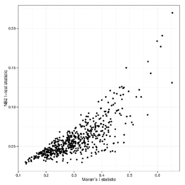
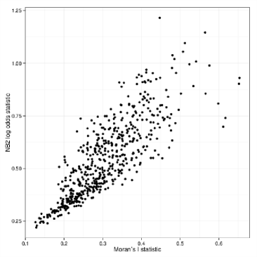
Figure 1: Comparison of this neighbor-based bootstrapping (NB2) method with Moran’s I statistic for detecting spatial autocorrelation. We show the NB2 experiment’s ability to detect spatial correlation (y-axis) measured by the paired Student’s t-test estimate (left) and the log odds estimate (right) for the neighbor county predictions vs random county predictions plotted against the Moran’s I statistic estimate (x-axis).

We rank ordered the ICD-9 codes using the two NB2 method implementations and the Moran’s I statistic to produce three ordered lists of ICD-9 codes from the strongest spatial correlation (largest Moran’s I statistic, largest NB2 t-test, largest NB2 log odds test) to the weakest. Tables Comparison with Moran’s I statistic - Comparison with Moran’s I statistic contain the top 25 ICD-9 codes for both NB2 implementations and Moran’s I. Here we will compare the properties of the spatial distributions for ICD-9 codes ranked highly by the two NB2 procedures with those ranked highly by Moran’s I statistic.

Table 1: Top 25 ICD-9 codes as ranked by NB2 (t-test)

[tabular=—c —c — c — l — c — r — l—, table head = NB2 (t-test) NB2 (odds) Moran ICD-9 diagnosis name ICD-9 Range Sill
, table foot = ] Table1.txt1=, 2=, 3=, 4=, 5=, 6=, 7=, 8=,9=,10=

Table 2: Top 25 ICD-9 codes as ranked by NB2 (log odds)

[tabular=—c —c — c — l — c — r — l—, table head = NB2 (odds) NB2 (t-test) Moran ICD-9 diagnosis name ICD-9 Range Sill
, table foot = ] Table2.txt1=, 2=, 3=, 4=, 5=, 6=, 7=, 8=, 9=,10=

Table 3: Top 25 ICD-9 codes as ranked by Moran’s I

[tabular=—c —c — c — l — c — r — l—, table head = Moran NB2 (t-test) NB2 (odds) ICD-9 diagnosis name ICD-9 Range Sill
, table foot = ] Table3.txt1=, 2=, 3=, 4=, 5=, 6=, 7=, 8=,9=, 10=

Scale of spatial influence

We applied a geostatistical ordinary kriging procedure using the R package automap to fit semivariograms models describing the spatial variation across the continental US for the incidence rates of each of the ICD-9 diagnostic codes. The semivariograms show the mean semivariance of values in binned separation distances between all pairs of spatial points. Here we use as input values the log incidence of the given ICD-9 in a county and approximate the spatial location of the observation as the county population centroid given by the US 2010 Census.

The semivariogram describes the distance within which the incidence rate is spatially autocorrelated. At separation distances where the semivariance is low, points have similar incidence rates. To quantify the size of spatial variation, we fit exponential semivariogram models to the data. The semivariogram model range describes the distance at which the model flattens to a constant semivariance. The semivariogram model sill describes the semivariance value at the range.

In Figure 2, we show two sample semivariograms, one for an ICD-9 code ranked highly by both the NB2 t-test implementation and Moran’s I (219: Other benign neoplasms of uterus) but relatively low by the NB2 log odds implementations and one for an ICD-9 code ranked highly by both the NB2 log odds implementation and Moran’s I but relatively low by the NB2 t-test implementation (477: Allergic rhinitis). The semivariogram model for 219 has a steep rise that quickly flattens (shorter range), and the semivariogram model for 477 continues to rise at large distance. The incidence rate maps in the bottom of Figure 2 correspondingly show smaller, high peaked cluster patterns of spatial variation for 219 (top left) and a larger scale gradation for 477 (top right).

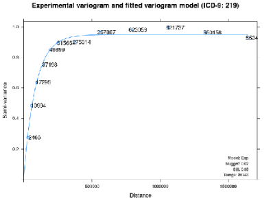
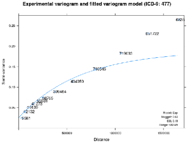
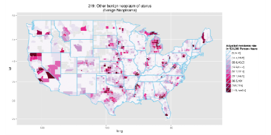
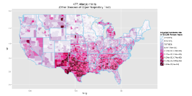
Figure 2: Example semivariograms and incidence rate maps for two ICD-9 codes. Top: Semivariograms for ICD-9 219, Other benign neoplasms of uterus, (left) and 477, Allergic rhinitis, (right). Bottom: Corresponding incidence rate maps.

We compare the results of semivariogram modeling for the highest ranked ICD-9 codes using the two NB2 method implementations to the semivariogram models for the highest ranked ICD-9 codes using Moran’s I statistic. Specifically, we compare average semivariogram model properties between groups of the top $N$ ranked ICD-9 codes for increasing values of $N$ using the two NB2 rankings and Moran’s I ranking. We will refer to $N$ as the rank threshold. In the top of Figure 3 (left), we show the mean semivariogram range vs the rank threshold $N$ using the NB2 method with t-test comparison (black) and Moran’s I statistic (grey). This shows the average distance range within which the incidence rates are autocorrelated for the top $N$ ranked ICD-9 codes by each method. For example, the mean semivariogram model range for the top 25 ICD-9 codes ranked by the NB2 method is 495 km vs 625 km for the top 25 Moran’s I statistic rankings. For the top 100 ICD-9 codes, the mean semivariogram model range is 404 km and 509 km for the NB2 method with t-test comparison and Moran’s I statistic, respectively. Generally, the NB2 method using the t-test comparison implementation ranks more highly ICD-9 codes showing spatial variation with smaller ranges, or smaller areas of autocorrelation.

In the bottom of Figure 3 (left), for comparison we show the same plot of the highest ranking semivariogram range properties for the NB2 method with log odds comparison (black) and Moran’s I statistic (grey). Generally, the NB2 method using the log odds comparison implementation ranks more highly ICD-9 codes showing spatial variation with larger ranges, or larger regions of autocorrelation.

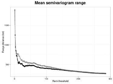
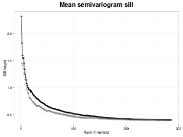
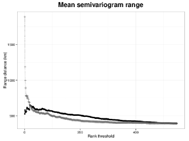
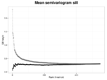
Figure 3: Average semivariogram properties for groups of top $N$ ICD-9 codes by the NB2 and Moran’s I methods. We show the mean range (left) and mean sill (right) for both the NB2 method (black points; top: t-test implementation, bottom: log odds implementation) and Moran’s I statistic (grey crosses) plotted against the rank threshold $N$. Compared to Moran’s I, the NB2 method with t-test implementation ranks more highly spatial variation with smaller ranges (autocorrelation within smaller distances) and larger sills (greater variance), whereas the NB2 method with log odds implementation ranks more highly spatial variation with larger ranges (autocorrelation within larger distances) and smaller sills (lower variance).

In the top of Figure 3 (right), we show the mean semivariogram sill vs the rank threshold $N$ using the NB2 t-test implementation (black) and Moran’s I statistic (grey). This essentially shows an estimate of the average variance in incidence rates across the US for the top $N$ ranked ICD-9 codes by each method. For example, the mean sill for the top 25 ICD-9 codes ranked by the NB2 method is 0.85 vs 0.67 for the top 25 Moran’s I statistic rankings. For the top 100 ICD-9 codes, the mean semivariogram model sill is 0.52 and 0.42 for the NB2 method t-test implementation and Moran’s I statistic, respectively. In this case the NB2 t-test implementation generally ranks more highly ICD-9 codes with larger variance in the incidence rates across the US.

In the bottom of Figure 3 (right), we show the same plot of the highest ranking semivariogram sill properties for the NB2 method with log odds comparison (black) and Moran’s I statistic (grey). Generally, the NB2 method using the log odds comparison implementation ranks more highly the autocorrelated ICD-9 codes with smaller variance.

DISCUSSION

There are many possible explanations for spatial patterns in the incidence rates of ICD-9 EMR data, and the rank ordering of ICD-9 codes with the described methods does not attempt to attribute any inferred pattern to a specific cause or suggest that the spatial variation is due to a physical environmental factor. Rather, we provide here a spatial autocorrelation method that can be implemented in multiple ways depending on the type of spatial pattern of interest. This flexibility is useful given that different categories of underlying factors as well as categories of disease can manifest as different spatial patterns, as we discuss below.

Incidence levels of diseases are influenced by a variety of factors, including:

• Physical environment — Some diseases are known to be related to the physical environment.

• Socioeconomic environment — The incidence levels of some diseases are impacted by socioeconomic or regional cultural differences.

• Structural environment - The incidence levels of some diseases reflect in part geospatial differences in insurance, provider billing or reimbursement patterns, local regulations, and related factors.

We show several incidence rate maps in Figure 4 as examples of patterns corresponding to these three types. These ICD-9 codes are all ranked in the top 25 according to at least one implementation of the NB2 method. In the top left is a map showing ICD-9 code 088: Other arthropod-borne diseases, which includes Lyme disease, a disease carried by ticks and known to have a regional concentration in the northeastern US and western Wisconsin areas. We consider this as an example of an ICD-9 code with spatial variation due to the physical environment. In the top right is a map showing ICD-9 code 635: Legally induced abortion. The spatial variation for this ICD-9 code shows clear delineation of the borders between states, which is likely to be due to differences in the structural environment. The delineation is particularly apparent on the borders between California and Nevada and New York and Pennsylvania. In the bottom left of Figure 4 is a map showing ICD-9 code 402: Hypertensive heart disease, which is the ICD-9 code ranked highest by the NB2 method. The spatial variation shows a pattern of higher incidence rate across a large crescent in the southern US. Given this cross-state regionally concentrated pattern, we define this to be an example of differences in the socioeconomic environment. In the bottom right we show a map of ICD-9 code 763: Fetus or newborn affected by other complications of labor and delivery, which is not easily classified as the previous three examples.

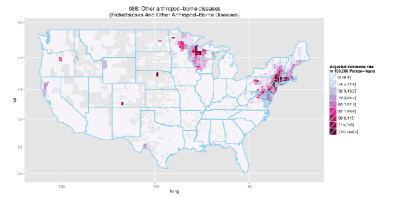
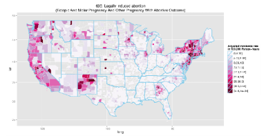
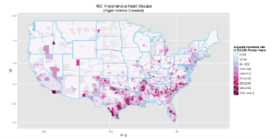
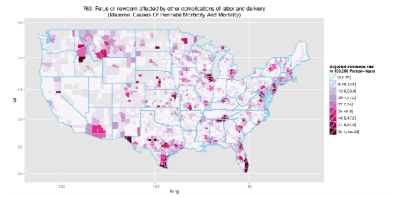
Figure 4: Incidence maps for several ICD-9 codes with different types of spatial variation. We show here 088: Other arthropod-borne diseases, (top left); 635: Legally induced abortion, (top right); 402: Hypertensive heart disease, (bottom left); and 763: Fetus or newborn affected by other complications of labor and delivery, (bottom right).

Characteristics of disease categories

In building semivariogram models describing the spatial variation for each ICD-9 code, we also looked at the model properties for categories of disease collectively. We grouped the ICD-9 codes according to standard categories, for example, 001-139 Infectious and Parasitic Diseases, 140-239 Neoplasms, etc. For each group we found the mean semivariogram model range, excluding ICD-9 codes where the semivariogram model range fit failed to iterate beyond the initial starting value, which leaves 286 individual ICD-9 codes in 17 categories. In Figure 5, we show a box plot of the semivariogram model ranges for each category ordered by increasing mean range.

There is no correlation between the mean semivariogram model ranges of categories and the number of ICD-9 codes grouped into each category. The categories with the fewest remaining ICD-9 codes are Symptoms, Signs, and Ill-defined Conditions (3 codes), Diseases of the Blood and Blood-forming Organs (6 codes), and Diseases of the Skin and Subcutaneous Tissue (8 codes). The categories of Neoplasms and Infectious and Parasitic Diseases have the most codes with 29 and 26 codes, respectively. However, the diseases with the smallest ranges generally also have low mean incidence rates across the US.

Given the variation of typical range values across different disease categories, one or the other presented implementation of the NB2 method may be appropriate for the detection of a spatial pattern for the type of disease of interest.

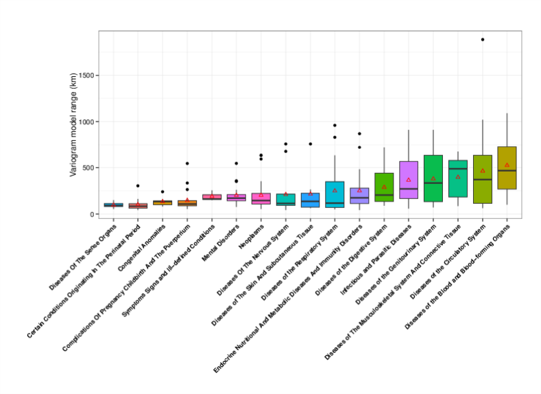
Figure 5: Box plot of variogram model ranges for categories of ICD-9 codes. The categories are in increasing order by the average variogram model range (marked by red triangles) for each category.

CONCLUSIONS

We have described here a bootstrap method that can be implemented multiple ways for detecting patterns in spatial variation based upon a region’s neighbors. The Neighbor-based Bootstrapping (NB2) method is a procedure for quantifying how much more accurate an estimate of the value of interest is based on values from bootstrapped neighboring units than bootstrapped randomly chosen units.

We have compared two implementations of the NB2 method to Moran’s I statistic for measuring spatial autocorrelation. Generally, the NB2 method and Moran’s I statistic are in rough agreement although with some scatter and interesting differences. Looking at the rank orderings of ICD-9 code county incidence rates across the US ranked by the NB2 method and by Moran’s I statistic shows that, by choosing one or the other implementation of the NB2 method, we can favor spatial variation with autocorrelation within smaller distances or of larger scale. Compared with Moran’s I statistic, the NB2 method allows more flexibility in controlling the type of spatial autocorrelation of interest.

Compared to Moran’s I statistic, the NB2 method using the t-test comparison ranks more highly the ICD-9 codes that appear to have multiple small clusters over a region whereas the NB2 method using a log odds comparison ranks more highly the ICD-9 codes with large regional gradients. We also compared the spatial properties of categories of disease by looking at the mean fitted semivariogram properties of each category and found that different categories of disease as a whole may have larger or smaller size scales of autocorrelation, as measured by average semivariogram model ranges. For example, ICD-9 codes related to conditions originating in the perinatal period generally have spatial variation that is autocorrelated within smaller distance ranges than ICD-9 codes related to diseases of the blood and blood-forming organs. Given this difference in spatial variation scale, one or the other implementation of the NB2 method may be more appropriate depending on the category of disease.

ACKNOWLEDGMENTS

This material is based in part upon work supported by the National Science Foundation under Grant Number 1129076 and the The National Cancer Institute (NCI) under Contract NIH/Leidos Biomedical Research, Inc. 13XS021 / HHSN261200800001E.

This work made use of the Open Science Data Cloud (OSDC), managed by the Open Commons Consortium (OCC) and funded in part by grants from the Gordon and Betty Moore Foundation [37].

AUTHOR DISCLOSURE STATEMENT

No competing financial interests exist.

SUPPLEMENTARY MATERIAL

In these supplementary materials we describe the results of the NB2 rankings by disease category and describe and spatial patterning for those ICD-9 codes ranked highly by either the NB2 t-test or odds implementation.

Infectious and Parasitic Diseases (001$-$139)

Of all the disease categories, Infectious and Parasitic Diseases have the highest average NB2 rank (most spatially significant) using the paired t-test implementation. In the box plot of Figure 5 this category includes 26 remaining ICD-9 codes with a mean semivariogram distance range of 365 km. Four of these diagnoses codes are ranked in the top 10 by the t-test implementation of the NB2 method. Two of these are animal related diseases, including 088: Other arthropod-borne diseases, which includes tick-borne Lyme disease with a geographic pattern in the Northeastern US and Wisconsin areas as shown in Figure 4 and 115: Histoplasmosis, also known as Ohio Valley disease, which is a fungal infection commonly spread by bat and bird droppings in soil. Histoplasmosis is also spatially interesting by the odds implementation of NB2, ranked 34.5. The other two codes are sexually transmitted infections which mainly spread the southern regional area of the US: 131: Trichomoniasis and 099: Other venereal diseases, which also shows a pattern due to the structural environment with high incidence in the state of Michigan.

Neoplasms (140$-$239)

Neoplasms as a group on average are ranked in the bottom half of the diseases categories (less spatially significant) by both implementations of NB2. The highest ranked ICD-9 code is 219: Other benign neoplasm of uterus, ranked 6 by t-test, with a small range of 90 km. There are 29 codes in Figure 5 with a mean range of 200 km. The codes with the largest range (outliers in Figure 5) are 173: Other malignant neoplasm of skin, ranked 130 by t-test and 98 by odds, with a large range of 635 km, affecting the southeastern US and the western and northeastern coastal areas. ICD-9 codes 189: Malignant neoplasm of kidney and other and unspecified urinary organs and 203: Multiple myeloma and immunoproliferative neoplasms also have large outlying ranges but have low NB2 ranks.

Endocrine, Nutritional, Metabolic, and Immunity Disorders (240$-$279)

This category of diseases has the third highest average NB2 rank using the t-test, 9th using odds, a mean range of 250 km, and several diagnosis codes in this category are ranked in the top 50 by NB2 with t-test. These include 268: Vitamin D deficiency, ranked 19, which has clusters of higher incidence in central Virginia, northern New York, southern Texas, central New Mexico, and the northwestern coast of the US; 259: Other endocrine disorders, ranked 24, which has small clusters in the southern and western US and also shows a pattern due to the structural environment with high incidence in Michigan; 257: Testicular dysfunction, ranked 29, which has a large range (outlier in Figure 5 at 720 km) with broadly affected regional areas in the south and also the west coast; and 266: Deficiency of b-complex components, ranked 38, has high incidence clusters in the Kentucky, Tennessee, Alabama, Georgia area. Additionally, 251: Other disorders of pancreatic internal secretion, which is ranked 52, is also an outlier in Figure 5 with a large range of 720 km. Using the odds NB2 implementation, 272: Disorders of lipoid metabolism is ranked highest at 11, and 250: Diabetes mellitus is next highest, ranking 22.5.

Diseases of the Blood and Blood-forming Organs (280$-$289)

This category of diagnosis codes has the largest average semivariogram range (525 km). The top ranked codes by NB2 are 281: Other deficiency anemias, ranked 15 with t-test and 63 with odds, 280: Iron deficiency anemias, ranked 60 with t-test and 42 with odds, and 285: Other and unspecified anemias, ranked 101 with t-test and 21 with odds, all of which show large-scale gradients with higher incidence in the south and southeast.

Mental Disorders (290$-$319)

The 19 ICD-9 codes in Figure 5 have a smaller range on average (200 km). The top NB2 ranked codes are 309: Adjustment reaction, ranked 65 with odds and 87.5 with t-test, which is most prominent in the northeast, northwest, and Michigan; 302: Sexual and gender identity disorders, ranked 65 by t-test and 196 by odds, with high incidence in the states of Georgia, South Carolina, and Nevada; and 304: Drug dependence, ranked 66 by t-test and 172.5 by odds, with high incidence in regions of Kentucky, Tennessee, and Alabama.The highest range outlier is 290: Dementias, which shows a strong signature of differences in the structural environment with high incidence in the states of Massachusetts and California and sharp state borders.

Diseases of the Nervous System (320$-$359)

This category of ICD-9 codes has a similar mean distance range to Neoplasms and Diseases of the Skin and Subcutaneous Tissue (210 km). The top NB2 ranked codes are 356: Hereditary and idiopathic peripheral neuropathy, ranked 93.5 using the t-test and 92.5 using odds, which has a higher than average range (760 km) reflecting a gradient of high incidence in the south and southeast;and 347: Cataplexy and narcolepsy, ranked 107 using the t-test and 370 using odds, which has clusters of high incidence primarily in central Ohio, central Indiana, Michigan, and South Carolina. The ICD-9 code 357: Inflammatory and toxic neuropathy also has a large outlying range (675 km) with higher incidence generally in Texas, Nevada, and the southeastern US.

Diseases of the Sense Organs (360$-$389)

The ICD-9 codes in this category were ranked relatively low by NB2 (least spatially significant) and also have the smallest average range of autocorrelation (95 km). The highest ranking code is 367: Disorders of refraction and accommodation, ranked 35 by the t-test and 89.5 by odds, which has higher incidence generally in the northwestern border states, central Illinois, southern Georgia, and in the states of Connecticut and Nevada.

Circulatory System (390$-$459)

This category of ICD-9 codes is the third highest ranked as spatially interesting using the mean of the NB2 t-test method results. Many codes in this category are ranked in the top 20. This category also has the second largest average semivariogram model range (465 km), meaning large spatial areas are autocorrelated. The top ranking codes using the odds NB2 implementation include 401: Essential hypertension, ranked 1 using the odds method and 171 using the t-test method, which shows a gentle gradient affecting the whole US with higher incidence in the southern region; 424: Other diseases of endocardium, ranked 7 using odds and 21 using the t-test, which also shows a gradient with higher incidence in the south and also some clustered areas; and 414: Other forms of chronic ischemic heart disease, ranked 12 by odds and 108, which is also more prevalent in the south. The top ranking codes using the t-test are 402: Hypertensive heart diseases, ranked 1 using the t-test and 19 using odds, which has high incidence in a large arc across the southern US shown in Figure 4; 413: Angina pectoris, ranked 7 using the t-test and 9 using odds, which has high incidence primarily in the south central US, Texas, and Florida; and 411: Other acute and subacute forms of ischemic heart disease, ranked 13 using the t-test and 30 using odds, which also has high incidence in the south central and east north central region US.

Respiratory System (460$-$519)

The NB2 method ranks the diagnosis codes in this category on average highly, the second highest group by the t-test and 4th by odds. The mean semivariogram range for the 25 codes shown in Figure 5 is 250 km with a large spread in the distribution. Several codes are ranked in the top 25: 514: Pulmonary congestion and hypostasis, ranked 18 by t-test and 21 by odds, which has higher incidence in the central and southern US; 487: Influenza, ranked 21 by t-test and 8 by odds, which has higher incidence in the southern US, excluding Florida, and a large range (830 km, high outlier); and 476: Chronic laryngitis and laryngotracheitis, ranked 25 by t-test and 231.5 by odds, which has smaller (55 km semivariogram range) clusters across the US. Allergic rhinitis (ICD-9 477) is also ranked second highest using the NB2 odds method, 47th using the t-test, and affects all of the US but is generally more prominent in the southern US. Chronic bronchitis (ICD-9 491) has the highest range (960 km) and is ranked 33 with higher incidence generally in the central US.

Digestive System (520$-$579)

Diseases in this category are mid ranked by NB2. The top ranked codes using the odds method are 530: Diseases of the esophagus, ranked 5 by odds and 149 by t-test, which shows generally higher incidence in the south and southeastern US; 535: Gastritis and duodenitis, ranked 13 by odds and 56 by t-test, which also is more prevalent in the southern areas with some smaller clustering; and 564 Functional digestive disorders not elsewhere classified, ranked 25.5 by odds and 98 by t-test, which again shows broad higher incidence in the south and southeast. The top ranked codes using the t-test method are 520: Disorders of tooth development and eruption, ranked 10.5 by t-test and 32 by odds, which shows sharp state outlines indicating differences in the structural environment with high incidence in Tennessee, Wisconsin, Pennsylvania, New Jersey, Delaware, Maine, and Michigan in particular; and 533: Peptic ulcer site unspecified, ranked 39 by t-test and 210.5 by odds, which generally has higher incidence in small clusters around the central and southern US .

Genitourinary System (580$-$629)

This category is ranked relatively high by both NB2 implementations (3rd by odds and 5th by t-test) and also has a higher average semivariogram range (380 km). The highest rank ICD-9 code in this category is 627: Menopausal and postmenopausal disorders, ranked 4 by odds and 70 by t-test, which has high incidence in large areas, particularly in the southern states as well as Montana and Michigan. Other ICD-9 codes with high ranks include 616: Inflammatory disease of the cervix, vagina, and vulva, ranked 6 by odds and 75 by t-test, which shows higher incidence generally in the southern states; 599: Other disorders of urethra and urinary tract, ranked 10 by odds and 261.5 by t-test, which also shows higher incidence in southern states; and 602: Other disorders of the prostate, ranked 9 by t-test and 202 by odds, which has high incidence regions primarily in southern Georgia, Texas, and the areas of Michigan, Ohio, Pennsylvania, New Jersey, and Maryland. Redundant prepuce and phimosis (ICD-9 605) is ranked 27 by t-test and 164 by odds and has several clusters of high incidence primarily in Texas and southern states, as well as central Illinois, northeastern Indiana, and Michigan. Inflammatory disease of ovary, fallopian tube, pelvic cellular tissue, and peritoneum (ICD-9 614) is ranked 41 by t-test and 64 by odds with a large range (910 km).

Pregnancy, Childbirth, and the Puerperium (630$-$679)

Complications of Pregnancy, Childbirth, and the Puerperium are mid ranked by the NB2 method, and this category has a small average range (145 km). The highest ranked codes are 635: Legally induced abortion, ranked 3 by t-test and 48 by odds, which shows clear state boundaries reflecting different structural environments and has a subsequently larger outlying range (335 km); 662: Long labor, ranked 17 by t-test and 254.5 by odds, which has dense clusters of high incidence in Texas, Florida, Georgia, Michigan, Wisconsin, and Montana with very low incidence elsewhere; and 645: Late pregnancy, ranked 43.5 by t-test and 146 by odds, which has higher incidence generally in the northern half of the US.

Skin and Subcutaneous Tissue (680$-$709)

This category of diseases is ranked in the bottom half of the categories (least spatially significant) by the NB2 method and has an average semivariogram range of 215 km. The top codes in this category are 682: Other cellulitis and abscess, ranked 3 with odds and 81 with t-test, which has higher incidence in the south central US and 692: Contact dematitis and other eczema, ranked 14 with odds and 165.5 with t-test, which has higher incidence in large areas in the mid central US, Michigan, California, Montana, and eastern and southeastern states. The ICD-9 code 680: Carbuncle and furuncle, ranked 106 by t-test and 182 by odds, has a large 760 km range (outlier in Figure 5). This code has a pattern of higher incidence generally in one primary main region centered around Louisiana and the Gulf Coast area and falling off with increasing distance. A smaller region in the area of eastern Montana and North Dakota also shows high incidence.

Musculoskeletal System and Connective Tissue (710$-$739)

The diagnosis codes in this category have a large average semivariogram range and are generally ranked of low spatial importance by NB2. The highest ranking code is 739: Nonallopathic lesions not elsewhere classified, ranked 8 with the t-test and 28 with odds, which shows clear state borders with high incidence in the northwestern states, particularly North Dakota, and also Iowa and Maine.

Congenital Anomalies (740$-$759)

The diagnosis codes in this category have a small average semivariogram range and are also generally ranked of low spatial importance by the NB2 method. The top code according to NB2 rankings is 743: Congenital anomalies of eye, ranked 128.5 by the t-test and 366.5 by odds. The ICD-9 code 754: Certain congenital musculoskeletal deformities has a higher than average range for this category (240 km), with high incidence and sharp borders in the state of Michigan.

Conditions Originating in the Perinatal Period (760$-$779)

Two codes for perinatal conditions rank in the top 50 by NB2. Fetus or newborn affected by other complications of labor and delivery (ICD-9 763) is ranked 14 by the t-test and 252.5 by odds and has small (range 60 km) clusters of high incidence in a dozen or so regions around the US, some crossing state borders, and low incidence elsewhere. Disorders relating to long gestation and high birthweight (ICD-9 766) is ranked 48 by the t-test and 296 by odds and shows similar smaller clustering in some areas.

Symptoms and Nonspecific Abnormal Findings (780$-$799)

On average these codes are ranked low by the NB2 t-test method but are ranked as the category with the most spatial autocorrelation by the Moran’s I statistic and by the NB2 odds method, several codes ranked in the top 20. These include 785: Symptoms involving cardiovascular symptoms, ranked 15 by odds and 245.5 by the t-test, 789: Other symptoms involving abdomen and pelvis, ranked 16 by odds and 401.5 by the t-test, and 786: Symptoms involving the respiratory system, ranked 17 by odds and 431 by the t-test, all of which cover most of the US with slightly higher incidence in the southern states and Michigan; The highest ranking ICD-9 code by the NB2 t-test method is 799: Other ill-defined and unknown causes of morbidity and mortality, ranked 93.5 using the t-test and 182 using odds, which has a high level of incidence in the state of Nevada and also has clusters of high incidence in Texas, Florida, New York, California, north central Illinois, and central Missouri.

References

- 1. Friedman, D. J., Parrish, R. G. & Ross, D. A. Electronic health records and us public health: Current realities and future promise. American J. Public Health 103, 1560 – 1567 (2013). URL http://proxy.uchicago.edu/login?url=http://search.ebscohost.com/login.aspx?direct=true&db=a9h&AN=89604054&site=ehost-live&scope=site.
- 2. Murdoch, T. & Detsky, A. The inevitable application of big data to health care. JAMA 309, 1351–1352 (2013). URL +http://dx.doi.org/10.1001/jama.2013.393. /data/Journals/JAMA/926712/jvp130007_1351_1352.pdf.
- 3. Brownstein, J. S., Freifeld, C. C. & Madoff, L. C. Digital disease detection: Harnessing the web for public health surveillance. N. Engl. J. Med. 360, 2153–2157 (2009). URL http://dx.doi.org/10.1056/NEJMp0900702. PMID: 19423867, http://dx.doi.org/10.1056/NEJMp0900702.
- 4. Salathe, M. et al. Digital epidemiology. PLoS Comput. Biol. 8, e1002616 (2012).
- 5. Generous, N., Fairchild, G., Deshpande, A., Del Valle, S. Y. & Priedhorsky, R. Global disease monitoring and forecasting with wikipedia. PLoS Comput. Biol. 10, e1003892 (2014).
- 6. Elliott, P. & Wartenberg, D. Spatial epidemiology: current approaches and future challenges. Environ. Health Perspect. 998–1006 (2004).
- 7. Rushton, G. et al. Geocoding health data: the use of geographic codes in Cancer Prev. Control, research and practice (CRC Press, 2007).
- 8. Beale, L., Abellan, J. J., Hodgson, S. & Jarup, L. Methodologic issues and approaches to spatial epidemiology. Environ Health Perspect 116, 1105–1110 (2008).
- 9. Cromley, E. K. & McLafferty, S. L. GIS and Public Health (Guilford Press, 2011).
- 10. Noble, D., Smith, D., Mathur, R., Robson, J. & Greenhalgh, T. Feasibility study of geospatial mapping of chronic disease risk to inform public health commissioning. BMJ open 2, e000711 (2012).
- 11. Becker, K. M., Glass, G. E., Brathwaite, W. & Zenilman, J. M. Geographic epidemiology of gonorrhea in baltimore, maryland, using a geographic information system. American J. Epidemiol. 147, 709–716 (1998).
- 12. Tiefelsdorf, M. The identification and analysis of spatial relationships in regression residuals by means of moran’s i (germany). Modelling spatil processes (1998).
- 13. Moran, P. A. Notes on continuous stochastic phenomena. Biometrika 17–23 (1950).
- 14. Ripley, B. D. Spatial statistics, vol. 575 (John Wiley & Sons, 2005).
- 15. Kitron, U. Landscape ecol. and epidemiology of vector-borne diseases: tools for spatial analysis. J. Med. Entomol. 35, 435–445 (1998).
- 16. Hay, S., Omumbo, J., Craig, M. & Snow, R. Earth observation, geographic information systems and plasmodium falciparum malaria in sub-saharan africa. Adv. Parasitol. 47, 173–215 (2000).
- 17. Moonan, P. K. et al. Using gis technology to identify areas of tuberculosis transmission and incidence. InterNatl. J. (Wash.) of Health Geographics 3, 23 (2004).
- 18. Sasaki, S., Suzuki, H., Igarashi, K., Tambatamba, B. & Mulenga, P. Spatial analysis of risk factor of cholera outbreak for 2003–2004 in a peri-urban area of lusaka, zambia. The American J. Trop. Med. Hyg. 79, 414–421 (2008).
- 19. Kamadjeu, R. Tracking the polio virus down the congo river: a case study on the use of google earth? in public health planning and mapping. InterNatl. J. (Wash.) of Health Geographics 8, 4 (2009).
- 20. Nuckols, J. R., Ward, M. H. & Jarup, L. Using geographic information systems for exposure assessment in environmental epidemiology studies. Environ. Health Perspect. 1007–1015 (2004).
- 21. Weis, B. K. et al. Personalized exposure assessment: promising approaches for human environ. health research. Environ. Health Perspect. 840–848 (2005).
- 22. Huang, Y.-L. & Batterman, S. Residence location as a measure of environmental exposure: a review of air pollution epidemiology studies. J. Expo. Anal. Environ. Epidemiol. 10, 66–85 (1999).
- 23. Jarup, L. Health and environment information systems for exposure and disease mapping, and risk assessment. Environ. Health Perspect. 995–997 (2004).
- 24. Graves, B. A. Integrative literature review: a review of literature related to geographical information systems, healthcare access, and health outcomes. Perspectives in health Inf. Manage./AHIMA, American Health Inf. Manage. Association 5 (2008).
- 25. Dean, H. D. & Fenton, K. A. Addressing social determinants of health in the prevention and control of hiv/aids, viral hepatitis, sex. transm. infect., and tuberculosis. Public Health Rep. 125, 1 (2010).
- 26. Harrison, K. M. & Dean, H. D. Use of data systems to address social determinants of health: a need to do more. Public Health Rep. 126, 1 (2011).
- 27. Gatrell, A. C. & Elliott, S. J. Geographies of health: an introduction (John Wiley & Sons, 2014).
- 28. Luther, S. L. et al. A method to measure the impact of prim. care programs targeted to reduce racial and ethnic disparities in health outcomes. J. Public Health Manag. Pract. 9, 243–248 (2003).
- 29. Geraghty, E. M., Balsbaugh, T., Nuovo, J. & Tandon, S. Using geographic information systems (gis) to assess outcome disparities in patients with type 2 diabetes and hyperlipidemia. The J. Am. Board Fam. Med. 23, 88–96 (2010). URL http://www.jabfm.org/content/23/1/88.abstract. http://www.jabfm.org/content/23/1/88.full.pdf+html.
- 30. Comer, K. F., Grannis, S., Dixon, B. E., Bodenhamer, D. J. & Wiehe, S. E. Incorporating geospatial capacity within clinical data systems to address social determinants of health. Public Health Rep. 126, 54 (2011).
- 31. Rodriguez, R. A., Hotchkiss, J. R. & O?Hare, A. M. Geographic information systems and chronic kidney disease: Racial disparities, rural residence and forecasting. Journal of nephrology 26, 3 (2013).
- 32. Rzhetsky, A. et al. Environmental and state-level regulatory factors affect the incidence of autism and intellectual disability. PLoS Comput Biol 10, e1003518 (2014). URL http://dx.doi.org/10.1371%2Fjournal.pcbi.1003518.
- 33. Klein, R. J., Schoenborn, C. A., for Health Statistics (US), N. C. et al. Age adjustment using the 2000 projected us population. CDC Statistical Notes (2001).
- 34. Day, J. C. Population projections of the United States, by age, sex, race, and Hispanic origin: 1992 to 2050. 1092 (US Department of Commerce, Economics and Statistics Administration, Bureau of the Census, 1992).
- 35. Waller, L. A. & Gotway, C. A. Applied spatial statistics for Public Health data, vol. 368 (John Wiley & Sons, 2004).
- 36. Bivand, R. S., Pebesma, E. & Gómez-Rubio, V. Applied Spatial Data Analysis with R (Springer New York, 2013).
- 37. Grossman, R. L. et al. The design of a community science cloud: The open science data cloud perspective. In SC Companion, 1051–1057 (IEEE Computer Society, 2012).