Detecting Multi-Spin Interactions
in the Inverse Ising Problem

Abstract

While the usual goal in Monte Carlo (MC) simulations of Ising models is the efficient generation of spin configurations with Boltzmann probabilities, the inverse problem is to determine the coupling constants from a given set of spin configurations. Most recent work has been limited to local magnetic fields and pair-wise interactions. We have extended solutions to multi-spin interactions, using correlation function matching (CFM). A more serious limitation of previous work has been the uncertainty of whether a chosen set of interactions is capable of faithfully representing real data. We show how our confirmation testing method uses an additional MC simulation to detect significant interactions that might be missing in the assumed representation of the data.

I Introduction

In many fields, such as biology, sociology, and neuroscience, obtaining information about underlying interactions between components of a system from observed correlations can clarify the structure of the system[1, 2, 3, 4, 5, 6, 7, 8, 9]. This reconstruction of cause from consequence is known as an inverse problem. Because of its relative simplicity, the inverse Ising model has become a standard test case for the development of methods to deal with intrinsically complex inverse problems. In 1984, a numerical solution to the problem was found by correlation function matching (CFM), using an identity due to Callen[10, 11, 12, 13]. At the time, the solution was only applied to transitionally invariant problems, but as we show below, the modifications to remove this restriction are trivial.

Recently, equations originally found with CFM were rediscovered by Aurell and Ekeberg, starting from different principles (pseudo-likelihood), and successfully applied to the Sherrington-Kirkpatrick (SK) model[9]. Their approach has the advantage of exhibiting the relationship of the solution to a Bayesian probability distribution on the space of the coupling constants. The CFM approach, on the other hand, clarifies the relationship between extracting information from the configurations and making inferences about the original coupling constants.

Recent work on inverse problems has been largely restricted to pairwise interactions, as in the SK model. We have extended it to include multi-spin interactions[10, 11, 12, 13], but there is still a question of whether a given set of real data can be faithfully represented by the chosen set of interactions. We answer this question by introducing a confirmation phase into our computations, using a new Monte Carlo (MC) simulation with the fitted coupling constants. By examining correlation functions that were not used in the inverse solution, we show that differences between the new MC simulation and the original data reveal neglected interactions. This “confirmation testing” provides a straightforward way of determining whether more interactions are needed for a faithful representation of the data, without having to perform a full computation of the coupling constants for the additional interactions. We will next describe the CFM equations that provide the basis for confirmation testing.

II CFM equations

To express a general, multi-spin Ising interaction, let $\alpha$ be a subset of $m_{\alpha}$ spins, and define the product of all spins in $\alpha$ as

$$S_{\alpha}=\prod_{j=1}^{m_{\alpha}}\sigma_{j}.$$ (1)

For each operator $S_{\alpha}$, we will assign a corresponding dimensionless coupling constant, $K_{\alpha}=\beta J_{\alpha}$, where $k_{B}$ is Boltzmann’s constant, $T$ is the temperature, and $\beta=1/k_{B}T$. The corresponding term in the dimensionless Hamiltonian $\mathcal{H}=-\beta H$, (where $H$ is the usual Hamiltonian) associated with $\alpha$ is $K_{\alpha}S_{\alpha}$. The full dimensionless Hamiltonian can then be written as a sum over the set of all spin products,

$$\mathcal{H}=\sum_{\alpha}K_{\alpha}S_{\alpha},$$ (2)

where the set $\textbf{K}=\{K_{\alpha}\}$, are the true values of the coupling constants.

We define an operator, $\mathcal{H}_{\ell}$, that includes all terms in the Hamiltonian containing a specific spin, $\sigma_{\ell}$[10, 11, 12]. If $\sigma_{\ell}\in\alpha$, we also define an operator $\widehat{S}_{\alpha,\ell}$ that omits the spin $\sigma_{\ell}$.

$$\widehat{S}_{\alpha,\ell}=S_{\alpha}/\sigma_{\ell}$$ (3)

If $\sigma_{\ell}\notin\alpha$, $\widehat{S}_{\alpha,\ell}=0$. The sum of all terms in the Hamiltonian that contain the “central” spin $\sigma_{\ell}$ is then

$$\mathcal{H}_{\ell}=\sigma_{\ell}\sum_{\alpha}K_{\alpha}\widehat{S}_{\alpha,\ell}.$$ (4)

The CFM method is based on fitting the correlation functions $c_{\alpha}\equiv\left\langle S_{\alpha}\right\rangle$ using an identity due to Callen[13].

$$c_{\alpha}\left(\textbf{K}\right)\equiv\left\langle\widehat{S}_{\alpha,\ell}\tanh\left[\sum_{\gamma}K_{\gamma}\widehat{S}_{\gamma,\ell}\right]\right\rangle=\left\langle S_{\alpha}\right\rangle$$ (5)

For comparison with earlier work, Eq. (5) corresponds to Eq. (14) in Ref. [10]. Aurell and Ekeberg considered $P(\sigma_{j})=(\sigma_{j}+1)/2$ instead of $\sigma_{j}$. Since the probability that a spin is positive is

$$P(+1)=\left(1-\exp\left[-2F_{\ell}\right]\right)^{-1}=\left(\tanh\left[F_{\ell}\right]+1\right)/2,$$ (6)

where $F_{\ell}=\sum_{\gamma}K_{\gamma}\widehat{S}_{\gamma,\ell}$, Eq. (5) is equivalent to Eq. (4) in Ref. [9].

Eq. (5) is exact for the correct values of the coupling constants and the exact correlation functions. Unfortunately, we never have the exact values of the correlation functions $c_{\alpha}=\left\langle S_{\alpha}\right\rangle$. Data always come from a finite sample, which we will take to be $N_{\textrm{MC}}$ spin configurations. We denote the corresponding approximate correlations functions as $\widehat{c}_{\alpha}=\left\langle S_{\alpha}\right\rangle_{MC}$. We can then use a modification of Eq. (5) to find a set of approximate coupling parameters $\widetilde{\textbf{K}}=\{\widetilde{K}_{\gamma}\}$ to fit the MC correlation functions.

$$\widehat{c}_{\alpha}\left(\widetilde{\textbf{K}}\right)\equiv\left\langle\widehat{S}_{\alpha,\ell}\tanh\left[\sum_{\gamma}\widetilde{K}_{\gamma}\widehat{S}_{\gamma,\ell}\right]\right\rangle_{MC}=\left\langle S_{\alpha}\right\rangle_{MC}$$ (7)

The equality in Eq. (7) will only hold for specific values of the coupling parameters $\widetilde{\textbf{K}}$. If trial values for the set $\widetilde{\textbf{K}}$ differ from the best-fitting value by $\delta\widetilde{\textbf{K}}=\{\delta K_{\alpha}\}$, an improved estimate can be obtained from a linearized approximation for the deviations from the best-fitting values.

$$\widehat{c}_{\alpha}\left(\widetilde{\textbf{K}}+\delta\widetilde{\textbf{K}}\right)-\left\langle S_{\alpha}\right\rangle_{MC}\approx\sum_{\beta}\frac{\partial\,\widehat{c}_{\alpha}\left(\widetilde{\textbf{K}}\right)}{\partial K_{\beta}}\,\delta\widetilde{K}_{\beta}$$ (8)

The derivatives in Eq. (8) are given by

$$\frac{\partial\,\widehat{c}_{\alpha}\left(\widetilde{\textbf{K}}\right)}{\partial K_{\beta}}=\left\langle\widehat{S}_{\alpha,\ell}\widehat{S}_{\beta,\ell}\,\textrm{sech}^{2}\left[\sum_{\gamma}\widetilde{K}_{\gamma}\widehat{S}_{\gamma,\ell}\right]\right\rangle_{MC}$$ (9)

Eq. (8) is iterated until convergence, which is quadratic in the absence of a degeneracy. Again for comparison with earlier work, Eqs. (9) corresponds to Eq. (15) in Ref. [10], and Eq. (7) in Ref. [9]. Note that for an interaction $\alpha$ with $m_{\alpha}$ spins, this procedure produces $m_{\alpha}$ values of $\widetilde{K}_{\alpha}$, one for each choice of the “central” spin $\sigma_{\ell}$. Before going on to confirmation testing, we next describe the application of the CFM solution to the inverse Ising problem, along with limitations that not only CFM, but any inverse method, will have with respect to recovering the true coupling constants. A virtue of the CFM is that it exposes these limitations clearly.

III The limited information contained in a set of configurations

There is an important distinction between extracting information contained in the configurations and inferring the values of the true couplings. For example, if $\mathcal{H}=h\sigma$, $\langle\sigma\rangle_{\text{exact}}=\tanh(h_{\text{exact}})$ is the exact average value of a spin $\sigma$ in a dimensionless field $h_{\text{exact}}$. Given $\langle\sigma\rangle_{\text{MC}}$ from an MC simulation, it is easy to find an effective magnetic field, $h_{\text{eff}}=\tanh^{-1}\langle\sigma\rangle_{\text{MC}}$, that reproduces it to arbitrary accuracy. Since $\langle\sigma\rangle_{\text{MC}}$ is not exactly equal to $\langle\sigma\rangle_{\text{exact}}$, $h_{\text{eff}}$ will differ from $h_{\text{exact}}$. The uncertainty in inferring $h_{\text{exact}}$ is given by $\delta h\approx\cosh(h)/\sqrt{N_{MC}}$. For small values of $h$, the error is approximately equal to the minimum error, $\delta h\approx\delta h_{\text{min}}=1/\sqrt{N_{MC}}$. Our simulation results have shown that the errors in estimating coupling constants at high temperatures are very close to the minimum error, even for large numbers of spins.

This simple estimate of $h_{\text{eff}}$ breaks down for $\langle\sigma\rangle_{\text{MC}}=1$ because it would imply that $h_{\text{eff}}=\infty$. A simple Bayesian argument suggests replacing $\langle\sigma\rangle_{\text{MC}}$ by $1-2/N_{\text{MC}}$, which gives a finite value for $h_{\text{eff}}$. Although this is a coarse method, it is quite effective for improving results. Aurell and Ekeberg used a similar strategy, but took the factor to be $0.999$ for all values of $N_{\text{MC}}$[9].

The limited information contained in the configurations is illustrated by the Sherrington-Kirkpatrick (SK) model of a spin glass[14]. In this model, there are $N$ spins, $\sigma=\{\sigma_{j}=\pm 1|j=1,2,\dots,N\}$, and the Hamiltonian is

$$H(\sigma)= -\sum_{j}b_{j}\sigma_{j}-\sum_{j>k}J_{j,k}\sigma_{j}\sigma_{k},$$ (10)

where the couplings $J_{j,k}$ have a quenched Gaussian distribution of width $J/\sqrt{N}$. The local magnetic fields $b_{j}$ can either be set equal to zero or given independent quenched values. The corresponding dimensionless coupling constants are $K_{j,k}=\beta J_{j,k}$ and $h_{j}=\beta b_{j}$.

The SK model is known to have a rugged energy landscape and a spin-glass phase transition at $k_{B}T_{c}=J$. This makes it very difficult to generate independent configurations at low temperatures, which limits the information carried by the configurations. However, it does not affect our ability to extract whatever information there is. While we must be careful in interpreting our results, predictions cannot be made more accurate without additional information.

For large systems at high temperatures, a different limitation comes from the minimum error for the correlation functions. Since the magnitude of the couplings goes as $1/\sqrt{N}$, the maximum temperature for which it is possible to determine the couplings to an accuracy of $\epsilon=\delta K_{\ell,j}/K_{\ell,j}$ is

$$T_{max}\lessapprox\frac{\epsilon J}{k_{B}}\sqrt{\frac{N_{MC}}{N}}.$$ (11)

To demonstrate that large coupling constants are not intrinsically difficult to determine – except for the factor of $\cosh(h)$ in the errors – we’ve carried out simulations with optimal sampling, that is, choosing independent random values for the spins at neighboring sites of a central site $\ell$. The values of $\sigma_{\ell}$ are then chosen with the thermal probability for a trial set of $K_{\ell,j}$’s. While the errors increase at low temperatures, good estimates of the original couplings can still be obtained for an SK distribution of quenched couplings down to $T=0.05\,T_{c}$, as shown in Table 1.

Table 1: Errors in estimates of original couplings from MC simulations for the toy model with random sampling. $n=N-1=49$ neighboring spins were independently assigned the values $\pm 1$ with equal probability. The true couplings were generated randomly from a Gaussian distribution with the width $\beta J/\sqrt{N}$ . The width of the actual distribution is given as $\Delta K$ in the second column. For these simulations, $N_{\text{MC}}=10^{5}$. The RMS error in the estimated couplings, given in the third column as $\delta K_{\ell,j}$, was found from the results of ten independent trials. The errors in the $K$’s were also compared to the minimum error $\delta_{min}=1/\sqrt{N_{\text{MC}}}=0.0032$ in the last column.

T	$\Delta K$	$\delta K_{\ell,j}$	$\delta K_{\ell,j}/K$	$\delta K_{\ell,j}/\delta_{min}$
10.0	0.0163	0.0099	0.609	0.99
2.0	0.0685	0.0034	0.50	1.08
1.0	0.1397	0.0041	0.029	1.29
0.5	0.2850	0.0053	0.0186	1.67
0.2	0.7186	0.0095	0.0132	3.01
0.1	1.3464	0.0160	0.0119	5.05
0.05	3.3452	0.0660	0.0197	20.9

The difficulties in extracting information from configurations generated below the critical temperature of the SK model are not due to any defect in the method of solution; the information is simply not available.

Because the low-temperature SK model has extremely long correlation times, MC simulations will usually only sample near a local free-energy minimum. For those states, it is common for some of the correlation functions to lock into values of $\pm 1$. When this happens, little information can be obtained about the corresponding interaction.

If we have the option to change the sampling method, restarting the simulations with different random initial conditions will generally improve results. Even though it is not possible to generate a complete sampling of a low-temperature spin glass in this manner, it can improve estimates of coupling constants.

The twin features of having small coupling constants for large systems and high temperatures, and a phase transition that limits information at low temperatures, leave only a small range of parameters for testing. This led us to use short-range models with multi-spin interactions to illustrate confirmation testing, as discussed in the following section.

IV Confirmation Testing

Any solution of the inverse Ising problem assumes a certain set of interactions that might be non-zero. When using confirmation testing, after fitting the coupling constants for those interactions, we perform an additional simulation using the fitted coupling constants to generate a new set of configurations. We then compare the correlation functions in the new set of configurations with those in the old set. If they match within the statistical errors discussed above, we have confirmed our assumptions. Deviations may reveal important interactions that were initially missing.

To illustrate confirmation testing, we have done MC simulations of a Hamiltonian with magnetic fields, nearest-neighbor pair interactions, and four-spin interactions on nearest-neighbor plaquettes on a $32\times 32$ lattice, with $N_{MC}=10^{5}$.

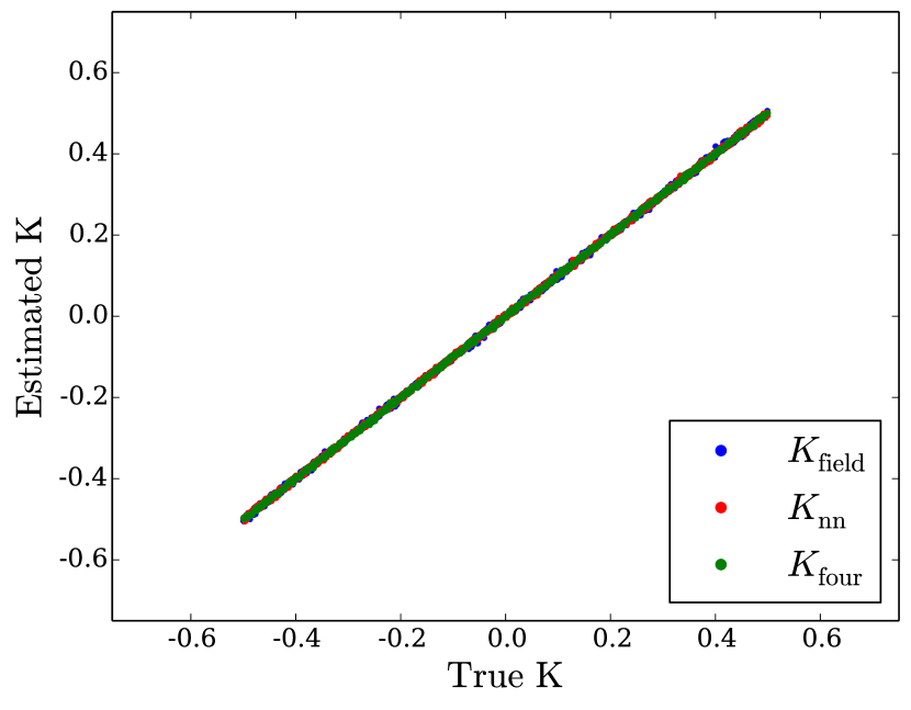
Figure 1: Plot of (well) estimated values of $h_{field}$, $K_{nn}$, and $K_{four}$ vs. their true values using data from an MC simulation on a $32\times 32$ lattice with $N_{MC}=10^{5}$. The true values of all coupling constants were generated from a uniform distribution in the range $[-0.5,0.5]$.

Fig. 1 shows that CFM accurately reproduces the values of the coupling constants for all types of interactions. Although it is not obvious from this plot, the errors in the four-spin coupling constants are smaller than those for the two-spin couplings, which are smaller than those for the local magnetic fields.

Next, we tried fitting our data with local magnetic fields and pairwise interactions, but omitting the four-spin couplings. Convergence was rapid, and the local magnetizations and the two-spin correlation functions were fit to better than $10^{-10}$. However, as can be seen in Fig. 2, the fitted values of the coupling constants deviated substantially from the true values.

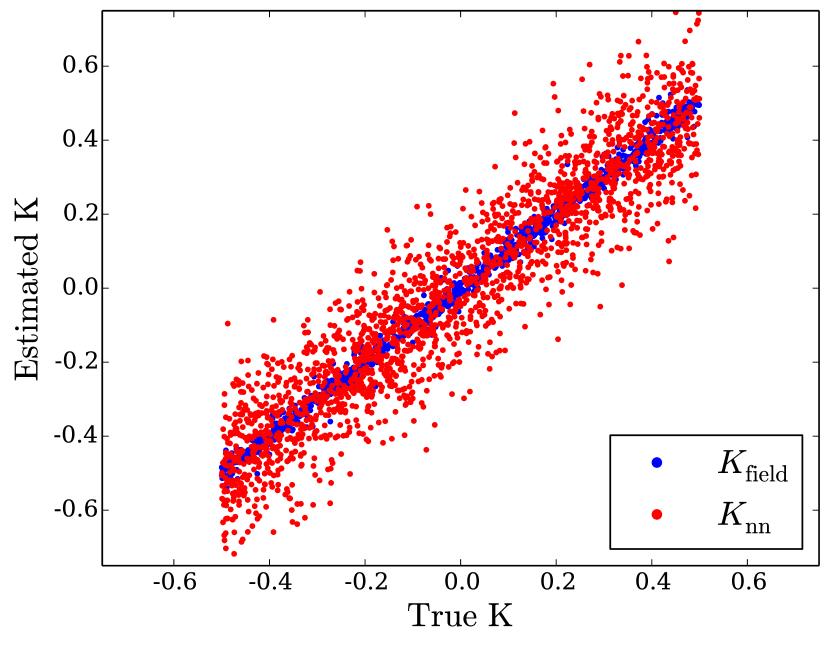
Figure 2: Plot of (badly) estimated coupling constants vs. the true values for the same MC simulation used in Fig. 1. While the estimates of the coupling constants only included nearest-neighbor interactions, the Hamiltonian of the MC simulation also included four-spin interactions. Omitting the four-spin couplings severely distorted the estimated values of $K_{field}$ and $K_{nn}$.

We carried out a confirmation simulation, using the local fields and two-spin couplings (but no four-spin terms) shown in Fig. 2. As expected, we found good agreement with the local magnetizations and two-spin correlation functions from the full Hamiltonian (with four-spin terms). However, we found poor agreement for the four-spin correlations, as shown in Fig. 3. Although the two-spin correlation functions and the local magnetizations agree to within the expected errors, there are significant differences in the four-spin correlations. For small values of the true four-spin coupling constants, the deviations are nearly linear, as expected. However, the linear approximation becomes worse as the magnitude of the true coupling constants increase. These systematic deviations demonstrate the existence of multi-spin couplings neglected in the initial assumptions.

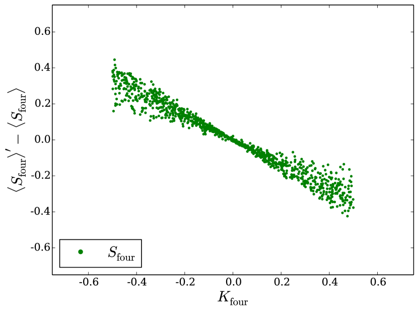
Figure 3: The two-spin coupling constants and the local magnetic fields shown in Fig. 2 were used in a new MC simulation on the same $32\times 32$ lattice with $N_{MC}=2.5\times 10^{5}$. This figure shows the differences in the four-spin correlation functions between the new simulation and the original data, plotted against the true values of the four-spin coupling constants.

V Conclusions

We have shown that multi-spin coupling constants can be accurately obtained in the inverse Ising problem with the CFM approach[10, 11, 12]. We have introduced and demonstrated confirmation testing, which uses a new MC simulation to confirm (or deny) whether a given set of effective coupling constants provides a faithful representation of real data.

References

- Schneidman et al. [2008] E. Schneidman, M. J. Berry II, R. Segev, and W. Bialek, “Weak pairwise correlations imply strongly correlated network states in a neural population,” Nature, 440, 1007–1012 (2008).
- Lezon et al. [2006] T. R. Lezon, J. R. Banavar, M. Cieplak, A. Maritan, and N. V. Fedoroff, “Using the principle of entropy maximization to infer genetic interaction networks from gene expression patterns,” Proc. Natl. Acad. Sci. U.S.A., 103, 19033–19038 (2006).
- Cocco et al. [2009] S. Cocco, S. Leibler, and R. Monasson, “Neuronal couplings between retinal ganglion cells inferred by efficient inverse statistical physics methods,,” Proc. Natl. Acad. Sci. U.S.A., 106, 14058–14062 (2009).
- Tkacik et al. [2006] G. Tkacik, E. Schneidman, M. J. Berry II, and W. Bialek, “Ising models for a network of real neurons,” (2006), arXiv:0912.5409.
- Tkacik et al. [2009] G. Tkacik, E. Schneidman, M. J. Berry II, and W. Bialek, “Spin glass models for a network of real neurons,” (2009), arXiv:0912.5409.
- Weigt et al. [2008] M. Weigt, R. A. White, H. Szurmant, J. A. Hoch, and T. Hwa, “Identification of direct residue contacts in protein protein interaction by message passing,” Proc. Natl. Acad. Sci. U.S.A., 106, 67–72 (2008).
- Schug et al. [2009] A. Schug, M. Weigt, J. N. Onuchic, T. Hwa, and H. Szurmant, “High-resolution protein complexes from integrating genomic information with molecular simulation,” Proc. Natl. Acad. Sci. U.S.A., 106, 22124–22129 (2009).
- Morcos et al. [2011] F. Morcos, A. Pagnani, B. Lunt, A. Bertolino, D. S. Marks, C. Sander, R. Zecchina, J. N. Onuchic, T. Hwa, and M. Weigt, “Direct-coupling analysis of residue coevolution captures native contacts across many protein families,” Proc. Natl. Acad. Sci. U.S.A., 108, E1293–E1301 (2011).
- Aurell and Ekeberg [2012] E. Aurell and M. Ekeberg, “Inverse ising inference using all the data,” Phys. Rev. Lett., 108, 090201 (2012).
- Swendsen [1984] R. H. Swendsen, “Monte Carlo calculation of renormalized coupling parameters,” Phys, Rev. Letters, 52, 1165 (1984a).
- Swendsen [1984] R. H. Swendsen, “Monte Carlo calculation of renormalized coupling parameters: I. d=2 Ising model,” Phys. Rev. B, 30, 3866 (1984b).
- Swendsen [1984] R. H. Swendsen, “Monte Carlo calculation of renormalized coupling parameters: II. d=3 Ising model,” Phys. Rev. B, 30, 3875 (1984c).
- Callen [1985] H. B. Callen, Thermodynamics and an Introduction to Thermostatistics, 2nd ed. (Wiley, New York, 1985).
- Sherrington and Kirkpatrick [1975] D. Sherrington and S. Kirkpatrick, “Solvable model of a spin-glass,” Phys. Rev. Lett., 35, 1792–1796 (1975).