Learn-and-Adapt Stochastic Dual Gradients for Network Resource Allocation

Abstract

Network resource allocation shows revived popularity in the era of data deluge and information explosion. Existing stochastic optimization approaches fall short in attaining a desirable cost-delay tradeoff. Recognizing the central role of Lagrange multipliers in network resource allocation, a novel learn-and-adapt stochastic dual gradient (LA-SDG) method is developed in this paper to learn the sample-optimal Lagrange multiplier from historical data, and accordingly adapt the upcoming resource allocation strategy. Remarkably, LA-SDG only requires just an extra sample (gradient) evaluation relative to the celebrated stochastic dual gradient (SDG) method. LA-SDG can be interpreted as a foresighted learning scheme with an eye on the future, or, a modified heavy-ball iteration from an optimization viewpoint. It is established - both theoretically and empirically - that LA-SDG markedly improves the cost-delay tradeoff over state-of-the-art allocation schemes.

I Introduction

In the era of big data analytics, cloud computing and Internet of Things, the growing demand for massive data processing challenges existing resource allocation approaches. Huge volumes of data acquired by distributed sensors in the presence of operational uncertainties caused by, e.g., renewable energy, call for scalable and adaptive network control schemes. Scalability of a desired approach refers to low complexity and amenability to distributed implementation, while adaptivity implies capability of online adjustment to dynamic environments.

Allocation of network resources can be traced back to the seminal work of [1]. Since then, popular allocation algorithms operating in the dual domain are first-order methods based on dual gradient ascent, either deterministic [2] or stochastic [3, 4]. Thanks to their simple computation and implementation, these approaches have attracted a great deal of recent interest, and have been successfully applied to cloud, transportation and power grid networks; see, e.g., [5, 6, 7, 8]. However, their major limitation is slow convergence, which results in high network delay. Depending on the application domain, the delay can be viewed as workload queuing time in a cloud network, traffic congestion in a transportation network, or energy level of batteries in a power network. To address this delay issue, recent attempts aim at accelerating first- and second-order optimization algorithms [9, 10, 11, 12]. Specifically, momentum-based accelerations over first-order methods were investigated using Nesterov [9], or, heavy-ball iterations [10]. Though these approaches work well in static settings, their performance degrades with online scheduling, as evidenced by the increase in accumulated steady-state error [13]. On the other hand, second-order methods such as the decentralized quasi-Newton approach and its dynamic variant developed in [11] and [12], incur high overhead to compute and communicate the decentralized Hessian approximations.

Capturing prices of resources, Lagrange multipliers play a central role in stochastic resource allocation algorithms [14]. Given abundant historical data in an online optimization setting, a natural question arises: Is it possible to learn the optimal prices from past data, so as to improve the performance of online resource allocation strategies? The rationale here is that past data contain statistics of network states, and learning from them can aid coping with the stochasticity of future resource allocation. A recent work in this direction is [15], which considers resource allocation with a finite number of possible network states and allocation actions. The learning procedure, however, involves constructing a histogram to estimate the underlying distribution of the network states, and explicitly solves an empirical dual problem. While constructing a histogram is feasible for a probability distribution with finite support, quantization errors and prohibitively high complexity are inevitable for a continuous distribution with infinite support.

In this context, the present paper aims to design a novel online resource allocation algorithm that leverages online learning from historical data for stochastic optimization of the ensuing allocation stage. The resultant approach, which we term “learn-and-adapt” stochastic dual gradient (LA-SDG) method, only doubles computational complexity of the classic stochastic dual gradient (SDG) method. With this minimal cost, LA-SDG mitigates steady-state oscillation, which is common in stochastic first-order acceleration methods [13, 10], while avoiding computation of the Hessian approximations present in the second-order methods [11, 12]. Specifically, LA-SDG only requires one more past sample to compute an extra stochastic dual gradient, in contrast to constructing costly histograms and solving the resultant large-scale problem [15].

The main contributions of this paper are summarized next.

1. Targeting a low-complexity online solution, LA-SDG only takes an additional dual gradient step relative to the classic SDG iteration. This step enables adapting the resource allocation strategy through learning from historical data. Meanwhile, LA-SDG is linked with the stochastic heavy-ball method, nicely inheriting its fast convergence in the initial stage, while reducing its steady-state oscillation.

2. The novel LA-SDG approach, parameterized by a positive constant $\mu$, provably yields an attractive cost-delay tradeoff $[\mu,\log^{2}(\mu)/\sqrt{\mu}]$, which improves upon the standard tradeoff $[\mu,{1}/{\mu}]$ of the SDG method [4]. Numerical tests further corroborate the performance gain of LA-SDG over existing resource allocation schemes.

Notation. $\mathbb{E}$ denotes the expectation operator, $\mathbb{P}$ stands for probability; $(\cdot)^{\top}$ stands for vector and matrix transposition, and $\|\mathbf{x}\|$ denotes the $\ell_{2}$-norm of a vector $\mathbf{x}$. Inequalities for vectors, e.g., $\mathbf{x}>\mathbf{0}$, are defined entry-wise. The positive projection operator is defined as $[a]^{+}:=\max\{a,0\}$, also entry-wise.

II Network Resource Allocation

In this section, we start with a generic network model and its resource allocation task in Section II-A, and then introduce a specific example of resource allocation in cloud networks in Section II-B. The proposed approach is applicable to more general network resource allocation tasks such as geographical load balancing in cloud networks [5], traffic control in transportation networks [7], and energy management in power networks [8].

II-A A unified resource allocation model

Consider discrete time $t\in\mathbb{N}$, and a network represented as a directed graph ${\cal G}=({\cal I},\,{\cal E})$ with nodes ${\cal I}:=\{1,\ldots,I\}$ and edges ${\cal E}:=\{1,\ldots,E\}$. Collect the workloads across edges $e=(i,j)\in{\cal E}$ in a resource allocation vector $\mathbf{x}_{t}\in\mathbb{R}^{E}$. The $I\times E$ node-incidence matrix is formed with the $(i,e)$-th entry

$$\mathbf{A}_{(i,e)}=\left\{\begin{array}[]{rl}{1,{}}&\text{if link $e$ enters node $i$}\\ {-1,{}}&\text{if link $e$ leaves node $i$}\\ {0,{}}&\text{else.}\end{array}\right.$$ (1)

We assume that each row of $\mathbf{A}$ has at least one $-1$ entry, and each column of $\mathbf{A}$ has at most one $-1$ entry, meaning that each node has at least one outgoing link, and each link has at most one source node. With $\mathbf{c}_{t}\in\mathbb{R}_{+}^{I}$ collecting the randomly arriving workloads of all nodes per slot $t$, the aggregate (endogenous plus exogenous) workloads of all nodes are $\mathbf{A}\mathbf{x}_{t}+\mathbf{c}_{t}$. If the $i$-th entry of $\mathbf{A}\mathbf{x}_{t}+\mathbf{c}_{t}$ is positive, there is service residual queued at node $i$; otherwise, node $i$ over-serves the current arrival. With a workload queue per node, the queue length vector $\mathbf{q}_{t}:=[q_{t}^{1},\ldots,q_{t}^{I}]^{\top}\in\mathbb{R}_{+}^{I}$ obeys the recursion

$$\mathbf{q}_{t+1}=\left[\mathbf{q}_{t}+\mathbf{A}\mathbf{x}_{t}+\mathbf{c}_{t}\right]^{+}\!,~{}\forall t$$ (2)

where $\mathbf{q}_{t}$ can represent the amount of user requests buffered in data queues, or energy stored in batteries, and $\mathbf{c}_{t}$ is the corresponding exogenously arriving workloads or harvested renewable energy of all nodes per slot $t$. Defining $\Psi_{t}(\mathbf{x}_{t}):=\Psi(\mathbf{x}_{t};\bm{\phi}_{t})$ as the aggregate network cost parameterized by the random vector $\bm{\phi}_{t}$, the local cost per node $i$ is $\Psi_{t}^{i}(\mathbf{x}_{t}):=\Psi^{i}(\mathbf{x}_{t};\bm{\phi}_{t}^{i})$, and $\Psi_{t}(\mathbf{x}_{t})=\sum_{i\in{\cal I}}\Psi_{t}^{i}(\mathbf{x}_{t})$. The model here is quite general. The duration of time slots can vary from (micro-)seconds in cloud networks, minutes in road networks, to even hours in power networks; the nodes can present the distributed front-end mapping nodes and back-end data centers in cloud networks, intersections in traffic networks, or, buses and substations in power networks; the links can model wireless/wireline channels, traffic lanes, and power transmission lines; while the resource vector $\mathbf{x}_{t}$ can include the size of data workloads, the number of vehicles, or the amount of energy.

Concatenating the random parameters into a random state vector $\mathbf{s}_{t}:=[\bm{\phi}_{t}^{\top},\mathbf{c}_{t}^{\top}]^{\top}$, the resource allocation task is to determine the allocation $\mathbf{x}_{t}$ in response to the observed (realization) $\mathbf{s}_{t}$ “on the fly,” so as to minimize the long-term average network cost subject to queue stability at each node, and operation feasibility at each link. Concretely, we have

$${\Psi}^{*}:= \min_{\{\mathbf{x}_{t},\forall t\}}\,\lim_{T\rightarrow\infty}\frac{1}{T}\sum_{t=1}^{T}\mathbb{E}\left[\Psi_{t}(\mathbf{x}_{t})\right]$$ (3a)

s.t. $$\mathbf{q}_{t+1}=\left[\mathbf{q}_{t}+\mathbf{A}\mathbf{x}_{t}+\mathbf{c}_{t}\right]^{+}\!,~{}\forall t$$ (3b)

$$\lim_{T\rightarrow\infty}\frac{1}{T}\sum_{t=1}^{T}\mathbb{E}\left[\mathbf{q}_{t}\right]<\infty$$ (3c)

$$~{}\mathbf{x}_{t}\in{\cal X}:=\{\mathbf{x}\,|\,\mathbf{0}\leq\mathbf{x}\leq\bar{\mathbf{x}}\},~{}\forall t$$ (3d)

where ${\Psi}^{*}$ is the optimal objective of problem (3), which includes also future information; $\mathbb{E}$ is taken over $\mathbf{s}_{t}:=[\bm{\phi}_{t}^{\top},\mathbf{c}_{t}^{\top}]^{\top}$ as well as possible randomness of optimization variable $\mathbf{x}_{t}$; constraints (3c) ensure queue stability; and (3d) confines the instantaneous allocation variables to stay within a time-invariant box constraint set ${\cal X}$, which is specified by, e.g., link capacities, or, server/generator capacities.

The queue dynamics in (3b) couple the optimization variables over an infinite time horizon, which implies that the decision variable at the current slot will have effect on all the future decisions. Therefore, finding an optimal solution of (3) calls for dynamic programming [16], which is known to suffer from the “curse of dimensionality” and intractability in an online setting. In Section III-A, we will circumvent this obstacle by relaxing (3b)-(3c) to limiting average constraints, and employing dual decomposition techniques.

II-B Motivating setup

The geographic load balancing task in a cloud network [5, 17, 18] takes the form of (3) with $J$ mapping nodes (e.g., DNS servers) indexed by ${\cal J}:=\{1,\ldots,J\}$, $K$ data centers indexed by ${\cal K}:=\{J+1,\ldots,J+K\}$. To match the definition in Section II-A, consider a virtual outgoing node (indexed by $0$) from each data center, and let $(k,0)$ represent this outgoing link. Define further the node set ${\cal I}:={\cal J}\bigcup{\cal K}$ that includes all nodes except the virtual one, and the edge set ${\cal E}:=\{(j,k),\forall j\!\in\!{\cal J},k\!\in\!{\cal K}\}\bigcup\{(k,0),\forall k\!\in\!{\cal K}\}$ that contains links connecting mapping nodes with data centers, and outgoing links from data centers.

Per slot $t$, each mapping node $j$ collects the amount of user data requests $c_{t}^{j}$, and forwards the amount $x_{t}^{jk}$ on its link to data center $k$ constrained by the bandwidth availability. Each data center $k$ schedules workload processing $x_{t}^{k0}$ according to its resource availability. The amount $x_{t}^{k0}$ can be also viewed as the resource on its virtual outgoing link $(k,0)$. The bandwidth limit of link $(j,k)$ is $\bar{x}^{jk}$, while the resource limit of data center $k$ (or link $(k,0)$) is $\bar{x}_{t}^{k0}$. Similar to those in Section II-A, we have the optimization vector $\mathbf{x}_{t}:=\{x_{t}^{ij},\,\forall(i,j)\!\in\!{\cal E}\}\!\in\!\mathbb{R}^{|\cal E|}$, $\mathbf{c}_{t}:=[c_{t}^{1},\ldots,c_{t}^{J},0\ldots,0]^{\top}\!\in\!\mathbb{R}^{J+K}$, and $\bar{\mathbf{x}}:=\{\bar{x}_{t}^{ij},\,\forall(i,j)\!\in\!{\cal E}\}\!\in\!\mathbb{R}^{|\cal E|}$. With these notational conventions, we have an $|{\cal I}|\times|{\cal E}|$ node-incidence matrix $\mathbf{A}$ as in (1). At each mapping node and data center, undistributed or unprocessed workloads are buffered in queues obeying (3b) with queue length $\mathbf{q}_{t}\in\mathbb{R}_{+}^{J+K}$; see also the system diagram in Fig. 1.

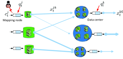
Figure 1: A diagram of online geographical load balancing. Per time $t$, mapping node $j$ has an exogenous workload $c_{t}^{j}$ plus that stored in the queue $q_{t}^{j}$, and schedules workload $x_{t}^{jk}$ to data center $k$. Data center $k$ serves an amount of workload $x_{t}^{k0}$ out of all the assigned $x_{t}^{jk}$ as well as that stored in the queue $q_{t}^{k}$. The thickness of each edge is proportional to its capacity.

Performance is characterized by the aggregate cost of power consumed at the data centers plus the bandwidth costs at the mapping nodes, namely

$$\Psi_{t}(\mathbf{x}_{t}):=\sum_{k\in{\cal K}}~{}\underbrace{~{}~{}\Psi_{t}^{k}(x_{t}^{k0})~{}~{}}_{\rm power~{}cost}~{}+~{}\sum_{j\in{\cal J}}\sum_{k\in{\cal K}}\underbrace{~{}~{}\Psi_{t}^{jk}(x_{t}^{jk})~{}~{}}_{\rm bandwidth~{}cost}.$$ (4)

The power cost $\Psi_{t}^{k}(x_{t}^{k0}):=\Psi^{k}(x_{t}^{k0};\bm{\phi}_{t}^{k})$, parameterized by the random vector $\bm{\phi}_{t}^{k}$, captures the local marginal price, and the renewable generation at data center $k$ during time period $t$. The bandwidth cost $\Psi_{t}^{jk}(x_{t}^{jk}):=\Psi^{jk}(x_{t}^{jk};\bm{\phi}_{t}^{jk})$, parameterized by the random vector $\bm{\phi}_{t}^{jk}$, characterizes the heterogeneous cost of data transmission due to spatio-temporal differences. To match the unified model in Section II-A, the local cost at data center $k\in{\cal K}$ is its power cost $\Psi_{t}^{k}(x_{t}^{k0})$, and the local cost at mapping node $j\in{\cal J}$ becomes $\Psi_{t}^{j}(\{x_{t}^{jk}\}):=\sum_{k\in{\cal K}}\Psi_{t}^{jk}(x_{t}^{jk})$. Hence, the cost in (4) can be also written as $\Psi_{t}(\mathbf{x}_{t}):=\sum_{i\in{\cal I}}\Psi_{t}^{i}(\mathbf{x}_{t})$. Aiming to minimize the time-average of (4), geographical load balancing fits the formulation in (3).

III Online Network Management via SDG

In this section, the dynamic problem (3) is reformulated to a tractable form, and classical stochastic dual gradient (SDG) approach is revisited, along with a brief discussion of its online performance.

III-A Problem reformulation

Recall in Section II-A that the main challenge of solving (3) resides in time-coupling constraints and unknown distribution of the underlying random processes. Regarding the first hurdle, combining (3b) with (3c), it can be shown that in the long term, workload arrival and departure rates must satisfy the following necessary condition [4, Theorem 2.8]

$$\lim_{T\rightarrow\infty}\frac{1}{T}\sum_{t=1}^{T}\mathbb{E}\left[\mathbf{A}\mathbf{x}_{t}+\mathbf{c}_{t}\right]\leq\mathbf{0}$$ (5)

given that the initial queue length is finite, i.e., $\|\mathbf{q}_{1}\|\leq\infty$. In other words, on average all buffered delay-tolerant workloads should be served. Using (5), a relaxed version of (3) is

$$\tilde{\Psi}^{*}:=\min_{\{\mathbf{x}_{t},\forall t\}}\,\lim_{T\rightarrow\infty}\frac{1}{T}\sum_{t=1}^{T}\mathbb{E}\left[\Psi_{t}(\mathbf{x}_{t})\right]~{}~{}\text{s.t.}~{}\eqref{eq.probl}~{}\text{and}~{}\eqref{Queue-relax}$$ (6)

where $\tilde{\Psi}^{*}$ is the optimal objective for the relaxed problem (6).

Compared to (3), problem (6) eliminates the time coupling across variables $\{\mathbf{q}_{t},\forall t\}$ by replacing (3b) and (3c) with (5). Since (6) is a relaxed version of (3) with the optimal objective $\tilde{\Psi}^{*}\leq{\Psi}^{*}$, if one solves (6) instead of (3), it will be prudent to derive an optimality bound on ${\Psi}^{*}$, provided that the sequence of solutions $\{\mathbf{x}_{t},\forall t\}$ obtained by solving (6) is feasible for the relaxed constraints (3b) and (3c). Regarding the relaxed problem (6), using arguments similar to those in [4, Theorem 4.5], it can be shown that if the random state $\mathbf{s}_{t}$ is independent and identically distributed (i.i.d.) over time $t$, there exists a stationary control policy $\bm{\chi}^{*}(\cdot)$, which is a pure (possibly randomized) function of the realization of random state $\mathbf{s}_{t}$ (or the observed state $\mathbf{s}_{t}$); i.e., it satisfies (3d), as well as guarantees that $\mathbb{E}[\Psi_{t}(\bm{\chi}^{*}(\mathbf{s}_{t}))]=\tilde{\Psi}^{*}$ and $\mathbb{E}[\mathbf{A}\bm{\chi}^{*}(\mathbf{s}_{t})+\mathbf{c}_{t}]\leq\mathbf{0}$. As the optimal policy $\bm{\chi}^{*}(\cdot)$ is time invariant, it implies that the dynamic problem (6) is equivalent to the following time-invariant ensemble program

$$\tilde{\Psi}^{*}:= \min_{\bm{\chi}(\cdot)}\;\mathbb{E}\left[\Psi\big{(}\bm{\chi}(\mathbf{s}_{t});\mathbf{s}_{t}\big{)}\right]$$ (7a)

s.t. $$\mathbb{E}[\mathbf{A}\bm{\chi}(\mathbf{s}_{t})+\mathbf{c}(\mathbf{s}_{t})]\leq\mathbf{0}$$ (7b)

$$\bm{\chi}(\mathbf{s}_{t})\in{\cal X},~{}\forall\mathbf{s}_{t}\in\mathcal{S}$$ (7c)

where $\bm{\chi}(\mathbf{s}_{t})\!:=\!\mathbf{x}_{t}$, $\mathbf{c}(\mathbf{s}_{t})=\mathbf{c}_{t}$, and $\Psi\big{(}\bm{\chi}(\mathbf{s}_{t});\mathbf{s}_{t}\big{)}\!:=\!\Psi_{t}(\mathbf{x}_{t})$; set $\mathcal{S}$ is the sample space of $\mathbf{s}_{t}$, and the constraint (7c) holds almost surely. Observe that the index $t$ in (7) can be dropped, since the expectation is taken over the distribution of random variable $\mathbf{s}_{t}$, which is time-invariant. Leveraging the equivalent form (7), the remaining task boils down to finding the optimal policy that achieves the minimal objective in (7a) and obeys the constraints (7b) and (7c). Note that the optimization in (7) is with respect to a stationary policy $\bm{\chi}(\cdot)$, which is an infinite dimensional problem in the primal domain. However, there is a finite number of expected constraints [cf. (7b)]. Thus, the dual problem contains a finite number of variables, hinting to the effect that solving (7) is tractable in the dual domain [19, 20].

III-B Lagrange dual and optimal policy

With $\bm{\lambda}\in\mathbb{R}_{+}^{I}$ denoting the Lagrange multipliers associated with (7b), the Lagrangian of (7) is

$${\cal L}(\bm{\chi},\bm{\lambda})\!:=\mathbb{E}\big{[}{\cal L}_{t}(\mathbf{x}_{t},\bm{\lambda})\big{]}$$ (8)

with $\bm{\lambda}\geq\mathbf{0}$, and the instantaneous Lagrangian is

$${\cal L}_{t}(\mathbf{x}_{t},\bm{\lambda})\!:= \Psi_{t}(\mathbf{x}_{t})+\bm{\lambda}^{\top}(\mathbf{A}\mathbf{x}_{t}+\mathbf{c}_{t})$$ (9)

where constraint (7c) remains implicit. Notice that the instantaneous objective $\Psi_{t}(\mathbf{x}_{t})$ and the instantaneous constraint $\mathbf{A}\mathbf{x}_{t}+\mathbf{c}_{t}$ are both parameterized by the observed state $\mathbf{s}_{t}:=[\bm{\phi}_{t}^{\top},\mathbf{c}_{t}^{\top}]^{\top}$ at time $t$; i.e., ${\cal L}_{t}(\mathbf{x}_{t},\bm{\lambda})={\cal L}(\bm{\chi}(\mathbf{s}_{t}),\bm{\lambda};\mathbf{s}_{t})$.

Correspondingly, the Lagrange dual function is defined as the minimum of the Lagrangian over the all feasible primal variables [21], given by

$${\cal D}(\bm{\lambda}): =\min_{\{\bm{\chi}(\mathbf{s}_{t})\in{\cal X},~{}\forall\mathbf{s}_{t}\in\mathcal{S}\}}\,{\cal L}(\bm{\chi},\bm{\lambda})$$

$$=\min_{\{\bm{\chi}(\mathbf{s}_{t})\in{\cal X},~{}\forall\mathbf{s}_{t}\in\mathcal{S}\}}\,\mathbb{E}\big{[}{\cal L}(\bm{\chi}(\mathbf{s}_{t}),\bm{\lambda};\mathbf{s}_{t})\big{]}.$$ (10a)

Note that the optimization in (10) is still w.r.t. a function. To facilitate the optimization, we re-write (10) relying on the so-termed interchangeability principle [shapiro2009, Theorem 7.80].

Lemma 1.

Let $\bm{\xi}$ denote a random variable on $\bm{\Xi}$, and ${\cal H}:=\{h(\,\cdot\,):\bm{\Xi}\rightarrow\mathbb{R}^{n}\}$ denote the function space of all the functions on $\bm{\Xi}$. For any $\bm{\xi}\in\bm{\Xi}$, if $f(\,\cdot\,,\bm{\xi}):\mathbb{R}^{n}\rightarrow\mathbb{R}$ is a proper and lower semicontinuous convex function, then it follows that

$$\min_{h(\cdot)\in{\cal H}}\,\mathbb{E}\big{[}f(h(\bm{\xi}),\bm{\xi})\big{]}=\mathbb{E}\left[\min_{\mathbf{h}\in\mathbb{R}^{n}}f(\mathbf{h},\bm{\xi})\right].$$ (10b)

Lemma 1 implies that under mild conditions, we can replace the optimization over a function space with (infinitely many) point-wise optimization problems. In the context here, we assume that $\Psi_{t}(\mathbf{x}_{t})$ is proper, lower semicontinuous, and strongly convex (cf. Assumption 2 in Section V). Thus, for given finite $\bm{\lambda}$ and $\mathbf{s}_{t}$, ${\cal L}(\,\cdot\,,\bm{\lambda};\mathbf{s}_{t})$ is also strongly convex, proper and lower semicontinuous. Therefore, applying Lemma 1 yields

$$\min_{\{\bm{\chi}(\cdot):{\cal S}\rightarrow{\cal X}\}}\!\!\!\mathbb{E}\big{[}{\cal L}(\bm{\chi}(\mathbf{s}_{t}),\bm{\lambda};\mathbf{s}_{t})\big{]}\!\!=\!\mathbb{E}\big{[}\!\min_{\bm{\chi}(\mathbf{s}_{t})\in{\cal X}}\!\!\!{\cal L}(\bm{\chi}(\mathbf{s}_{t}),\bm{\lambda};\mathbf{s}_{t})\big{]}\!\!\!\!$$ (10c)

where the minimization and the expectation are interchanged. Accordingly, we re-write (10) in the following form

$$\!\!\!{\cal D}(\bm{\lambda})\!=\!\mathbb{E}\!\left[\min_{\bm{\chi}(\mathbf{s}_{t})\in{\cal X}}\!{\cal L}(\bm{\chi}(\mathbf{s}_{t}),\bm{\lambda};\mathbf{s}_{t})\right]\!=\!\mathbb{E}\!\left[\min_{\mathbf{x}_{t}\in{\cal X}}{\cal L}_{t}(\mathbf{x}_{t},\bm{\lambda})\right]\!.\!\!$$ (10d)

Likewise, for the instantaneous dual function ${\cal D}_{t}(\bm{\lambda})={\cal D}(\bm{\lambda};\mathbf{s}_{t}):=\min_{\mathbf{x}_{t}\in{\cal X}}{\cal L}_{t}(\mathbf{x}_{t},\bm{\lambda})$, the dual problem of (7) is

$$\max_{\bm{\lambda}\geq\mathbf{0}}\,{\cal D}(\bm{\lambda}):=\mathbb{E}\left[{\cal D}_{t}(\bm{\lambda})\right].$$ (11)

In accordance with the ensemble primal problem (7), we will henceforth refer to (11) as the ensemble dual problem.

If the optimal Lagrange multiplier $\bm{\lambda}^{*}$ associated with (7b) were known, then optimizing (7) and consequently (6) would be equivalent to minimizing the Lagrangian ${\cal L}(\bm{\chi},\bm{\lambda}^{*})$ or infinitely many instantaneous $\{{\cal L}_{t}(\mathbf{x}_{t},\bm{\lambda}^{*})\}$, over the set ${\cal X}$ [16]. We restate this assertion as follows.

Proposition 1.

Consider the optimization problem in (7). Given a realization $\mathbf{s}_{t}$, and the optimal Lagrange multiplier $\bm{\lambda}^{*}$ associated with the constraints (7b), the optimal instantaneous resource allocation decision is

$$\mathbf{x}_{t}^{*}=\bm{\chi}^{*}(\mathbf{s}_{t})\in\arg\min_{\bm{\chi}(\mathbf{s}_{t})\in{\cal X}}{\cal L}(\mathbf{x}_{t},\bm{\lambda}^{*};\mathbf{s}_{t})$$ (12)

where $\in$ accounts for possibly multiple minimizers of ${\cal L}_{t}$.

When the realizations $\{\mathbf{s}_{t}\}$ are obtained sequentially, one can generate a sequence of optimal solutions $\{\mathbf{x}_{t}^{*}\}$ correspondingly for the dynamic problem (6). To obtain the optimal allocation in (12) however, $\bm{\lambda}^{*}$ must be known. This fact motivates our novel “learn-and-adapt” stochastic dual gradient (LA-SDG) method in Section IV. To this end, we will first outline the celebrated stochastic dual gradient iteration (a.k.a. Lyapunov optimization).

III-C Revisiting stochastic dual (sub)gradient

To solve (11), a standard gradient iteration involves sequentially taking expectations over the distribution of $\mathbf{s}_{t}$ to compute the gradient. Note that when the Lagrangian minimization (cf. (12)) admits possibly multiple minimizers, a subgradient iteration is employed instead of the gradient one [21]. This is challenging because the distribution of $\mathbf{s}_{t}$ is typically unknown in practice. But even if the joint probability distribution functions were available, finding the expectations is not scalable as the dimensionality of $\mathbf{s}_{t}$ grows.

A common remedy to this challenge is stochastic approximation [22, 4], which corresponds to the following SDG iteration

$$\bm{\lambda}_{t+1}~{}=\big{[}\bm{\lambda}_{t}+\mu\nabla{\cal D}_{t}(\bm{\lambda}_{t})\big{]}^{+},\;\forall t$$ (13a)

where $$\mu \nabla{\cal D}_{t}(\bm{\lambda}_{t})=\mathbf{A}\mathbf{x}_{t}+\mathbf{c}_{t} \mathbb{E}[\nabla{\cal D}_{t}(\bm{\lambda}_{t})]=\nabla{\cal D}(\bm{\lambda}_{t}) \mathbf{x}_{t} t$$ is a positive (and typically pre-selected constant) stepsize. The stochastic (sub)gradient is an unbiased estimate of the true (sub)gradient; that is, . Hence, the primal can be found by solving the following instantaneous sub-problems, one per

$$\mathbf{x}_{t}\in\arg\min_{\mathbf{x}_{t}\in{\cal X}}{\cal L}_{t}(\mathbf{x}_{t},\bm{\lambda}_{t}).$$ (13b)

The iterate $\bm{\lambda}_{t+1}$ in (13a) depends only on the probability distribution of $\mathbf{s}_{t}$ through the stochastic (sub)gradient $\nabla{\cal D}_{t}(\bm{\lambda}_{t})$. Consequently, the process $\{\bm{\lambda}_{t}\}$ is Markov with invariant transition probability when $\mathbf{s}_{t}$ is stationary. An interesting observation is that since $\nabla{\cal D}_{t}(\bm{\lambda}_{t}):=\mathbf{A}\mathbf{x}_{t}+\mathbf{c}_{t}$, the dual iteration can be written as [cf. (13a)]

$${\bm{\lambda}_{t+1}}/{\mu}=\left[{\bm{\lambda}_{t}}/{\mu}+\mathbf{A}\mathbf{x}_{t}+\mathbf{c}_{t}\right]^{+},\;\forall t$$ (14)

which coincides with (3b) for $\bm{\lambda}_{t}/\mu=\mathbf{q}_{t}$; see also [4, 14, 17] for a virtual queue interpretation of this parallelism.

Thanks to its low complexity and robustness to non-stationary scenarios, SDG is widely used in various areas, including adaptive signal processing [23], stochastic network optimization [4, 14, 15], and energy management in power grids [17, 8]. For network management in particular, this iteration entails a cost-delay tradeoff as summarized next; see e.g., [4].

Proposition 2.

If ${\Psi}^{*}$ is the optimal cost in (3) under any feasible control policy with the state distribution available, and if a constant stepsize $\mu$ is used in (13a), the SDG recursion (13) achieves an ${\cal O}(\mu)$-optimal solution in the sense that

$$\lim_{T\rightarrow\infty}\frac{1}{T}\sum_{t=1}^{T}\mathbb{E}\left[\Psi_{t}\left(\mathbf{x}_{t}(\bm{\lambda}_{t})\right)\right]\leq{\Psi}^{*}+{\cal O}(\mu)$$ (15a)

where $$\mathbf{x}_{t}(\bm{\lambda}_{t}) {\cal O}(1/\mu)$$ denotes the decisions obtained from (13b), and it incurs a steady-state queue length , namely

$$\lim_{T\rightarrow\infty}\frac{1}{T}\sum_{t=1}^{T}\mathbb{E}\left[\mathbf{q}_{t}\right]={\cal O}\left(\frac{1}{\mu}\right).$$ (15b)

Proposition 2 asserts that SDG with stepsize $\mu$ will asymptotically yield an ${\cal O}(\mu)$-optimal solution [21, Prop. 8.2.11], and it will have steady-state queue length $\mathbf{q}_{\infty}$ inversely proportional to $\mu$. This optimality gap is standard, because iteration (13a) with a constant stepsize will converge to a neighborhood of the optimum $\bm{\lambda}^{*}$ [23]. Under mild conditions, the optimal multiplier is bounded, i.e., $\bm{\lambda}^{*}={\cal O}(1)$, so that the steady-state queue length $\mathbf{q}_{\infty}$ naturally scales with ${\cal O}(1/{\mu})$ since it hovers around $\bm{\lambda}^{*}/\mu$; see (14). As a consequence, to achieve near optimality (sufficiently small $\mu$), SDG incurs large average queue lengths, and thus undesired average delay as per Little’s law [4]. To overcome this limitation, we develop next an online approach, which can improve SDG’s cost-delay tradeoff, while still preserving its affordable complexity and adaptability.

IV Learn-and-Adapt SDG

Our main approach is derived in this section, by nicely leveraging both learning and optimization tools. Its decentralized implementation is also developed.

IV-A LA-SDG as a foresighted learning scheme

The intuition behind our learn-and-adapt stochastic dual gradient (LA-SDG) approach is to incrementally learn network state statistics from observed data while adapting resource allocation driven by the learning process. A key element of LA-SDG could be termed as “foresighted” learning because instead of myopically learning the exact optimal argument from empirical data, LA-SDG maintains the capability to hedge against the risk of “future non-stationarities.”

Algorithm 1 LA-SDG for Stochastic Network Optimization

1:Initialize: dual iterate $\bm{\lambda}_{1}$, empirical dual iterate $\hat{\bm{\lambda}}_{1}$, queue length $\mathbf{q}_{1}$, control variable $\bm{\theta}=\sqrt{\mu}\log^{2}(\mu)\cdot\mathbf{1}$, and proper stepsizes $\mu$ and $\{\eta_{t},\,\forall t\}$.

2:for $t=1,2\dots$ do

3:     Resource allocation (1st gradient):

4:     Construct the effective dual variable via (17b), observe      the current state $\mathbf{s}_{t}$, and obtain resource allocation $\mathbf{x}_{t}(\bm{\gamma}_{t})$     by minimizing online Lagrangian (17a).

5:     Update the instantaneous queue length $\mathbf{q}_{t+1}$ via

$$\mathbf{q}_{t+1}=\big{[}\mathbf{q}_{t}+\big{(}\mathbf{A}\mathbf{x}_{t}(\bm{\gamma}_{t})+\mathbf{c}_{t}\big{)}\big{]}^{+},\;\forall t.$$ (16)

6:     Sample recourse (2nd gradient):

7:     Obtain variable $\mathbf{x}_{t}(\hat{\bm{\lambda}}_{t})$ by solving online Lagrangian     minimization with sample $\mathbf{s}_{t}$ via (18b).

8:     Update the empirical dual variable $\hat{\bm{\lambda}}_{t+1}$ via (18a).

9:end for

The proposed LA-SDG is summarized in Algorithm 1. It involves the queue length $\mathbf{q}_{t}$ and an empirical dual variable $\hat{\bm{\lambda}}_{t}$, along with a bias-control variable $\bm{\theta}$ to ensure that LA-SDG will attain near optimality in the steady state [cf. Theorems 2 and 3]. At each time slot $t$, LA-SDG obtains two stochastic gradients using the current $\mathbf{s}_{t}$: One for online resource allocation, and another one for sample learning/recourse. For the first gradient (lines 3-5), contrary to SDG that relies on the stochastic multiplier estimate $\bm{\lambda}_{t}$ [cf. (13b)], LA-SDG minimizes the instantaneous Lagrangian

$$\mathbf{x}_{t}(\bm{\gamma}_{t})\in\arg\min_{\mathbf{x}_{t}\in{\cal X}}{\cal L}_{t}(\mathbf{x}_{t},\bm{\gamma}_{t})$$ (17a)

which depends on what we term effective multiplier, given by

$$\!\underbrace{~{}~{}~{}~{}\bm{\gamma}_{t}~{}~{}~{}~{}}_{\rm effective~{}multiplier}=\underbrace{~{}~{}~{}~{}\hat{\bm{\lambda}}_{t}~{}~{}~{}~{}}_{\rm statistical~{}learning}+~{}~{}\underbrace{~{}~{}~{}\mu\mathbf{q}_{t}~{}-~{}\bm{\theta}~{}~{}~{}}_{\rm online~{}adaptation},\;\forall t.$$ (17b)

Variable $\bm{\gamma}_{t}$ also captures the effective price, which is a linear combination of the empirical $\hat{\bm{\lambda}}_{t}$ and the queue length $\mathbf{q}_{t}$, where the control variable $\mu$ tunes the weights of these two factors, and $\bm{\theta}$ controls the bias of $\bm{\gamma}_{t}$ in the steady state [15]. As a single pass of SDG “wastes” valuable online samples, LA-SDG resolves this limitation in a learning step by evaluating a second gradient (lines 6-8); that is, LA-SDG simply finds the stochastic gradient of (11) at the previous empirical dual variable $\hat{\bm{\lambda}}_{t}$, and implements a gradient ascent update as

$$\hat{\bm{\lambda}}_{t+1}=\big{[}\hat{\bm{\lambda}}_{t}+\eta_{t}\big{(}\mathbf{A}\mathbf{x}_{t}(\hat{\bm{\lambda}}_{t})+\mathbf{c}_{t}\big{)}\big{]}^{+},\;\forall t$$ (18a)

where $$\eta_{t} \mathbf{x}_{t}(\hat{\bm{\lambda}}_{t})$$ is a proper diminishing stepsize, and the “virtual” allocation can be found by solving

$$\mathbf{x}_{t}(\hat{\bm{\lambda}}_{t})\in\arg\min_{\mathbf{x}_{t}\in{\cal X}}{\cal L}_{t}(\mathbf{x}_{t},\hat{\bm{\lambda}}_{t}).$$ (18b)

Note that different from $\mathbf{x}_{t}(\bm{\gamma}_{t})$ in (17a), the “virtual” allocation $\mathbf{x}_{t}(\hat{\bm{\lambda}}_{t})$ will not be physically implemented. The multiplicative constant $\mu$ in (17b) controls the degree of adaptability, and allows for adaptation even in the steady state ($t\rightarrow\infty$), but the vanishing $\eta_{t}$ is for learning, as we shall discuss next.

The key idea of LA-SDG is to empower adaptive resource allocation (via $\bm{\gamma}_{t}$) with the learning process (effected through $\hat{\bm{\lambda}}_{t}$). As a result, the construction of $\bm{\gamma}_{t}$ relies on $\hat{\bm{\lambda}}_{t}$, but not vice versa. For a better illustration of the effective price (17b), we call $\hat{\bm{\lambda}}_{t}$ the statistically learnt price to obtain the exact optimal argument of the expected problem (11). We also call $\mu\mathbf{q}_{t}$ (which is exactly $\bm{\lambda}_{t}$ as shown in (13a)) the online adaptation term since it can track the instantaneous change of system statistics. Intuitively, a large $\mu$ will allow the effective policy to quickly respond to instantaneous variations so that the policy gains improved control of queue lengths, while a small $\mu$ puts more weight on learning from historical samples so that the allocation strategy will incur less variance in the steady state. In this sense, LA-SDG can attains both statistical efficiency and adaptability.

Distinctly different from SDG that combines statistical learning with resource allocation into a single adaptation step [cf. (13a)], LA-SDG performs these two tasks into two intertwined steps: resource allocation (17), and statistical learning (18). The additional learning step adopts diminishing stepsize to find the “best empirical” dual variable from all observed network states. This pair of complementary gradient steps endows LA-SDG with its attractive properties. In its transient stage, the extra gradient evaluations and empirical dual variables accelerate the convergence speed of SDG; while in the steady stage, the empirical multiplier approaches the optimal one, which significantly reduces the steady-state queue lengths.

Remark 1.

Readers familiar with algorithms on statistical learning and stochastic network optimization can recognize their similarities and differences with LA-SDG.

(P1) SDG in [4] involves only the first part of LA-SDG ($1$st gradient), where the allocation policy purely relies on stochastic estimates of Lagrange multipliers or instantaneous queue lengths, i.e., $\bm{\gamma}_{t}=\mu\mathbf{q}_{t}$. In contrast, LA-SDG further leverages statistical learning from streaming data.

(P2) Several schemes have been developed recently for statistical learning at scale to find $\hat{\bm{\lambda}}_{t}$, namely, SAG in [24] and SAGA in [25]. However, directly applying $\bm{\gamma}_{t}=\hat{\bm{\lambda}}_{t}$ to allocate resources causes infeasibility. For a finite time $t$, $\hat{\bm{\lambda}}_{t}$ is $\delta$-optimal for (11), and the primal variable $\mathbf{x}_{t}(\hat{\bm{\lambda}}_{t})$ in turn is $\delta$-feasible with respect to (7b) that is necessary for (3c). Since $\mathbf{q}_{t}$ essentially accumulates online constraint violations of (7b), it will grow linearly with $t$ and eventually become unbounded.

IV-B LA-SDG as a modified heavy-ball iteration

The heavy-ball iteration belongs to the family of momentum-based first-order methods, and has well-documented acceleration merits in the deterministic setting [26]. Motivated by its convergence speed in solving deterministic problems, stochastic heavy-ball methods have been also pursued recently [13, 10].

The stochastic version of the heavy-ball iteration is [13]

$$\bm{\lambda}_{t+1}=\bm{\lambda}_{t}+\mu\nabla{\cal D}_{t}(\bm{\lambda}_{t})+\beta(\bm{\lambda}_{t}-\bm{\lambda}_{t-1}),\;\forall t$$ (19)

where $\mu>0$ is an appropriate constant stepsize, $\beta\in[0,1)$ denotes the momentum factor, and the stochastic gradient $\nabla{\cal D}_{t}(\bm{\lambda}_{t})$ can be found by solving (13b) using heavy-ball iterate $\bm{\lambda}_{t}$. This iteration exhibits attractive convergence rate during the initial stage, but its performance degrades in the steady state. Recently, the performance of momentum iterations (heavy-ball or Nesterov) with constant stepsize $\mu$ and momentum factor $\beta$, has been proved equivalent to SDG with constant ${\mu}/(1-\beta)$ per iteration [13]. Since SDG with a large stepsize converges fast at the price of considerable loss in optimality, the momentum methods naturally inherit these attributes.

To see the influence of the momentum term, consider expanding the iteration (19) as

$$\bm{\lambda}_{t+1} =\bm{\lambda}_{t}+\mu\nabla{\cal D}_{t}(\bm{\lambda}_{t})+\beta(\bm{\lambda}_{t}-\bm{\lambda}_{t-1})$$

$$=\bm{\lambda}_{t}+\mu\nabla{\cal D}_{t}(\bm{\lambda}_{t})\!+\!\beta\left[\mu\nabla{\cal D}_{t-1}(\bm{\lambda}_{t-1})\!+\!\beta(\bm{\lambda}_{t-1}\!-\!\bm{\lambda}_{t-2})\right]$$

$$=\bm{\lambda}_{t}+\underbrace{\mu\textstyle\sum_{\tau=1}^{t}\beta^{t-\tau}\nabla{\cal D}_{\tau}(\bm{\lambda}_{\tau})}_{\rm accumulated~{}gradient}+\underbrace{\beta^{t}(\bm{\lambda}_{1}\!-\!\bm{\lambda}_{0})}_{\rm initial~{}state}.$$ (20)

The stochastic heavy-ball method will accelerate convergence in the initial stage thanks to the accumulated gradients, and it will gradually forget the initial state. As $t$ increases however, the algorithm also incurs a worst-case oscillation ${\cal O}({\mu}/(1-\beta))$, which degrades performance in terms of objective values when compared to SDG with stepsize $\mu$. This is in agreement with the theoretical analysis in [13, Theorem 11].

Different from standard momentum methods, LA-SDG nicely inherits the fast convergence in the initial stage, while reducing the oscillation of stochastic momentum methods in the steady state. To see this, consider two consecutive iterations (17b)

$$\bm{\gamma}_{t+1} =\hat{\bm{\lambda}}_{t+1}+\mu\mathbf{q}_{t+1}-\bm{\theta}$$ (21a)

$$\bm{\gamma}_{t} =\hat{\bm{\lambda}}_{t}+\mu\mathbf{q}_{t}-\bm{\theta}$$ (21b)

and subtract them, to arrive at

$$\bm{\gamma}_{t+1} =\bm{\gamma}_{t}+\mu\left(\mathbf{q}_{t+1}-\mathbf{q}_{t}\right)+(\hat{\bm{\lambda}}_{t+1}-\hat{\bm{\lambda}}_{t})$$

$$=\bm{\gamma}_{t}+\mu\nabla{\cal D}_{t}(\bm{\gamma}_{t})+(\hat{\bm{\lambda}}_{t+1}-\hat{\bm{\lambda}}_{t}),~{}~{}~{}\forall t.$$ (22)

Here the equalities in (IV-B) follows from $\nabla{\cal D}_{t}(\bm{\gamma}_{t})=\mathbf{A}\mathbf{x}_{t}(\bm{\gamma}_{t})+\mathbf{c}_{t}$ in $\mathbf{q}_{t}$ recursion (16), and with a sufficiently large $\bm{\theta}$, the projection in (16) rarely (with sufficiently low probability) takes effect since the steady-state $\mathbf{q}_{t}$ will hover around $\bm{\theta}/\mu$; see the details of Theorem 2 and the proof thereof.

Comparing the LA-SDG iteration (IV-B) with the stochastic heavy-ball iteration (19), both of them correct the iterates using the stochastic gradient $\nabla{\cal D}_{t}(\bm{\gamma}_{t})$ or $\nabla{\cal D}_{t}(\bm{\lambda}_{t})$. However, LA-SDG incorporates the variation of a learning sequence (also known as a reference sequence) $\{\hat{\bm{\lambda}}_{t}\}$ into the recursion of the main iterate $\bm{\gamma}_{t}$, other than heavy-ball’s momentum term $\beta(\bm{\lambda}_{t}-\bm{\lambda}_{t-1})$. Since the variation of learning iterate $\hat{\bm{\lambda}}_{t}$ eventually diminishes as $t$ increases, keeping the learning sequence enables LA-SDG to enjoy accelerated convergence in the initial (transient) stage compared to SDG, while avoiding large oscillation in the steady state compared to the stochastic heavy-ball method. We formally remark this obervation next.

Remark 2.

LA-SDG offers a fresh approach to designing stochastic optimization algorithms in a dynamic environment. While directly applying the momentum-based iteration to a stochastic setting may lead to unsatisfactory steady-state performance, it is promising to carefully design a reference sequence that exactly converges to the optimal argument. Therefore, algorithms with improved convergence (e.g., the second-order method in [12]) can also be incorporated as a reference sequence to further enhance the performance of LA-SDG.

IV-C Complexity and distributed implementation of LA-SDG

This section introduces a fully distributed implementation of LA-SDG by exploiting the problem structure of network resource allocation. For notational brevity, collect the variables representing outgoing links from node $i$ in $\mathbf{x}_{t}^{i}:=\{x_{t}^{ij},\forall j\in{\cal N}_{i}\}$ with ${\cal N}_{i}$ denoting the index set of outgoing neighbors of node $i$. Let also $\mathbf{s}_{t}^{i}:=[\bm{\phi}_{t}^{i};c_{t}^{i}]$ denote the random state at node $i$. It will be shown that the learning and allocation decision per time slot $t$ is processed locally per node $i$ based on its local state $\mathbf{s}_{t}^{i}$.

To this end, rewrite the Lagrangian minimization for a general dual variable $\bm{\lambda}\in\mathbb{R}_{+}^{I}$ at time $t$ as [cf. (17a) and (18b)]

$$\min_{\mathbf{x}_{t}\in{\cal X}}\sum_{i\in{\cal I}}\Psi^{i}(\mathbf{x}_{t}^{i};\bm{\phi}_{t}^{i})+\sum_{i\in{\cal I}}\lambda^{i}(\mathbf{A}_{(i,:)}\mathbf{x}_{t}+c_{t}^{i})$$ (23)

where $\lambda^{i}$ is the $i$-th entry of vector $\bm{\lambda}$, and $\mathbf{A}_{(i,:)}$ denotes the $i$-th row of the node-incidence matrix $\mathbf{A}$. Clearly, $\mathbf{A}_{(i,:)}$ selects entries of $\mathbf{x}_{t}$ associated with the in- and out-links of node $i$. Therefore, the subproblem at node $i$ is

$$\min_{\mathbf{x}_{t}^{i}\in{\cal X}^{i}}\Psi^{i}(\mathbf{x}_{t}^{i};\bm{\phi}_{t}^{i})+\sum_{j\in{\cal N}_{i}}(\lambda^{j}-\lambda^{i})x_{t}^{ji}$$ (24)

where ${\cal X}^{i}$ is the feasible set of primal variable $\mathbf{x}_{t}^{i}$. In the case of (3d), the feasible set ${\cal X}$ can be written as a Cartesian product of sets $\{{\cal X}^{i},\forall i\}$, so that the projection of $\mathbf{x}_{t}$ to ${\cal X}$ is equivalent to separate projections of $\mathbf{x}_{t}^{i}$ onto ${\cal X}^{i}$. Note that $\{\lambda^{j},\forall j\in{\cal N}_{i}\}$ will be available at node $i$ by exchanging information with the neighbors per time $t$. Hence, given the effective multipliers $\gamma_{t}^{j}$ ($j$-th entry of $\bm{\gamma}_{t}$) from its outgoing neighbors in $j\in{\cal N}_{i}$, node $i$ is able to form an allocation decision $\mathbf{x}_{t}^{i}(\bm{\gamma}_{t})$ by solving the convex programs (24) with $\lambda^{j}=\gamma_{t}^{j}$; see also (17a). Needless to mention, $q_{t}^{i}$ can be locally updated via (16), that is

$$q_{t+1}^{i}=\left[q_{t}^{i}+\Big{(}\sum_{j:i\in{\cal N}_{j}}x^{ji}_{t}(\bm{\gamma}_{t})-\sum_{j\in{\cal N}_{i}}x^{ij}_{t}(\bm{\gamma}_{t})+c_{t}^{i}\Big{)}\right]^{+}$$ (25)

where $\{x^{ji}_{t}(\bm{\gamma}_{t})\}$ are the local measurements of arrival (departure) workloads from (to) its neighbors.

Likewise, the tentative primal variable $\mathbf{x}_{t}^{i}(\hat{\bm{\lambda}}_{t})$ can be obtained at each node locally by solving (24) using the current sample $\mathbf{s}_{t}^{i}$ again with $\lambda^{i}=\hat{\lambda}_{t}^{i}$. By sending $\mathbf{x}_{t}^{i}(\hat{\bm{\lambda}}_{t})$ to its outgoing neighbors, node $i$ can update the empirical multiplier $\hat{\lambda}_{t+1}^{i}$ via

$$\hat{\lambda}_{t+1}^{i}\!=\!\left[\hat{\lambda}_{t}^{i}\!+\!\eta_{t}\Big{(}\sum_{j:i\in{\cal N}_{j}}x^{ji}_{t}(\hat{\bm{\lambda}}_{t})\!-\!\sum_{j\in{\cal N}_{i}}x^{ij}_{t}(\hat{\bm{\lambda}}_{t})\!+\!c_{t}^{i}\Big{)}\right]^{+}$$ (26)

which, together with the local queue length $q_{t+1}^{i}$, also implies that the next $\gamma_{t+1}^{i}$ can be obtained locally.

Compared with the classic SDG recursion (13a)-(13b), the distributed implementation of LA-SDG incurs only a factor of two increase in computational complexity. Next, we will further analytically establish that it can improve the delay of SDG by an order of magnitude with the same order of optimality gap.

V Optimality and Stability of LA-SDG

This section presents performance analysis of LA-SDG, which will rely on the following four assumptions.

Assumption 1.

The state $\mathbf{s}_{t}$ is bounded and i.i.d. over time $t$.

Assumption 2.

$\Psi_{t}(\mathbf{x}_{t})$ is proper, $\sigma$-strongly convex, lower semi-continuous, and has $L_{\rm p}$-Lipschitz continuous gradient. Also, $\Psi_{t}(\mathbf{x}_{t})$ is non-decreasing w.r.t. all entries of $\mathbf{x}_{t}$ over ${\cal X}$.

Assumption 3.

There exists a stationary policy $\bm{\chi}(\cdot)$ satisfying $\bm{\chi}(\mathbf{s}_{t})\in{\cal X}$ for all $\mathbf{s}_{t}$, and $\mathbb{E}[\mathbf{A}\bm{\chi}(\mathbf{s}_{t})+\mathbf{c}_{t}]\leq-\bm{\zeta}$, where $\bm{\zeta}>\mathbf{0}$ is a slack vector constant.

Assumption 4.

For any time $t$, the magnitude of the constraint is bounded, that is, $\|\mathbf{A}\mathbf{x}_{t}+\mathbf{c}_{t}\|\leq M,\;\forall\mathbf{x}_{t}\in{\cal X}$.

Assumption 1 is typical in stochastic network resource allocation [14, 15, 27], and can be relaxed to an ergodic and stationary setting following [20, 28]. Assumption 2 requires the primal objective to be well behaved, meaning that it is bounded from below and has a unique optimal solution. Note that non-decreasing costs with increased resources are easily guaranteed with e.g., exponential and quadratic functions in our simulations. In addition, Assumption 2 ensures that the dual function has favorable properties, which are important for the ensuring stability analysis. Assumption 3 is Slater’s condition, which guarantees the existence of a bounded optimal Lagrange multiplier [21], and is also necessary for queue stability [4]. Assumption 4 guarantees boundedness of the gradient of the instantaneous dual function, which is common in performance analysis of stochastic gradient-type algorithms [29].

Building upon the desirable properties of the primal problem, we next show that the corresponding dual function satisfies both smoothness and quadratic growth properties [30, 31], which will be critical to the subsequent analysis.

Lemma 2.

Under Assumption 2, the dual function ${\cal D}(\bm{\lambda})$ in (11) is $L_{\rm d}$-smooth, where $L_{\rm d}=\rho(\mathbf{A}^{\top}\mathbf{A})/\sigma$, and $\rho(\mathbf{A}^{\top}\mathbf{A})$ denotes the spectral radius of $\mathbf{A}^{\top}\mathbf{A}$. In addition, if $\bm{\lambda}$ lies in a compact set, there always exists a constant $\epsilon$ such that ${\cal D}(\bm{\lambda})$ satisfies the following quadratic growth property

$${\cal D}(\bm{\lambda}^{*})-{\cal D}(\bm{\lambda})\geq\frac{\epsilon}{2}\|\bm{\lambda}^{*}-\bm{\lambda}\|^{2}$$ (27)

where $\bm{\lambda}^{*}$ is the optimal multiplier for the dual problem (11).

Proof.

See Appendix A. ∎

We start with the convergence of the empirical dual variables $\hat{\bm{\lambda}}_{t}$. Note that the update of $\hat{\bm{\lambda}}_{t}$ is a standard learning iteration from historical data, and it is not affected by future resource allocation decisions. Therefore, the theoretical result on SDG with diminishing stepsize is directly applicable [29, Sec. 2.2].

Lemma 3.

Let $\hat{\bm{\lambda}}_{t}$ denote the empirical dual variable in Algorithm 1, and $\bm{\lambda}^{*}$ the optimal argument for the dual problem (11). If the stepsize is chosen as $\eta_{t}=\frac{\alpha D}{M\sqrt{t}},\,\forall t$, with a constant $\alpha>0$, a sufficient large constant $D>0$, and $M$ as in Assumption 4, then it holds that

$$\mathbb{E}\left[{\cal D}(\bm{\lambda}^{*})\!-\!{\cal D}(\hat{\bm{\lambda}}_{t})\right]\leq\max\{\alpha,\alpha^{-1}\}\,\frac{DM}{\sqrt{t}}$$ (28)

where the expectation is over all the random states $\mathbf{s}_{t}$ up to $t$.

Lemma 3 asserts that using a diminishing stepsize, the dual function value converges sub-linearly to the optimal value in expectation. In principle, $D$ is the radius of the feasible set for the dual variable $\bm{\lambda}$ [29, Sec. 2.2]. However, as the optimal multiplier $\bm{\lambda}^{*}$ is bounded according to Assumption 3, one can always estimate a large enough $D$, and the estimation error will only affect the constant of the sub-optimality bound (28) through the scalar $\alpha$. The sub-optimality bound in Lemma 3 holds in expectation, which averages over all possible sample paths $\{\mathbf{s}_{1},\ldots,\mathbf{s}_{t}\}$.

As a complement to Lemma 3, the almost sure convergence of the empirical dual variables is established next to characterize the performance of each individual sample path.

Theorem 1.

For the sequence of empirical multipliers $\{\hat{\bm{\lambda}}_{t}\}$ in Algorithm 1, if the stepsizes are chosen as $\eta_{t}=\frac{\alpha D}{M\sqrt{t}},\forall t$, with constants $\alpha,M,D$ defined in Lemma 3, it holds that

$$\lim_{t\rightarrow\infty}\hat{\bm{\lambda}}_{t}=\bm{\lambda}^{*},\quad{\rm w.p.1}$$ (29)

where $\bm{\lambda}^{*}$ is the optimal dual variable for the expected dual function minimization (11).

Proof.

The proof follows the steps in [21, Proposition 8.2.13], which is omitted here. ∎

Building upon the asymptotic convergence of empirical dual variables for statistical learning, it becomes possible to analyze the online performance of LA-SDG. Clearly, the online resource allocation $\mathbf{x}_{t}$ is a function of the effective dual variable $\bm{\gamma}_{t}$ and the instantaneous network state $\mathbf{s}_{t}$ [cf. (17a)]. Therefore, the next step is to show that the effective dual variable $\bm{\gamma}_{t}$ also converges to the optimal argument of the expected problem (11), which would establish that the online resource allocation $\mathbf{x}_{t}$ is asymptotically optimal. However, directly analyzing the trajectory of $\bm{\gamma}_{t}$ is nontrivial, because the queue length $\{\mathbf{q}_{t}\}$ is coupled with the reference sequence $\{\hat{\bm{\lambda}}_{t}\}$ in $\bm{\gamma}_{t}$. To address this issue, rewrite the recursion of $\bm{\gamma}_{t}$ as

$$\bm{\gamma}_{t+1}=\bm{\gamma}_{t}+(\hat{\bm{\lambda}}_{t+1}-\hat{\bm{\lambda}}_{t})+\mu(\mathbf{q}_{t+1}-\mathbf{q}_{t}),\;\forall t$$ (30)

where the update of $\bm{\gamma}_{t}$ depends on the variations of $\hat{\bm{\lambda}}_{t}$ and $\mathbf{q}_{t}$. We will first study the asymptotic behavior of queue lengths $\mathbf{q}_{t}$, and then derive the analysis of $\bm{\gamma}_{t}$ using the convergence of $\hat{\bm{\lambda}}_{t}$ in (29), and the recursion (30).

Define the time-varying target $\tilde{\bm{\theta}}_{t}=\bm{\lambda}^{*}-\hat{\bm{\lambda}}_{t}+\bm{\theta}$, which is the optimality residual of statistical learning $\bm{\lambda}^{*}-\hat{\bm{\lambda}}_{t}$ plus the bias-control variable $\bm{\theta}$. Per Theorem 1, it readily follows that $\lim_{t\rightarrow\infty}\tilde{\bm{\theta}}_{t}=\bm{\theta},\,{\rm w.p.1}$. By showing that $\mathbf{q}_{t}$ is attracted towards the time-varying target $\tilde{\bm{\theta}}_{t}/\mu$, we will further derive the stability of queue lengths.

Lemma 4.

With $\mathbf{q}_{t}$ and $\mu$ denoting queue length and stepsize, there exists a constant $B=\Theta({1}/{\sqrt{\mu}})$, and a finite time $T_{B}<\infty$, such that for all $t\geq T_{B}$, if $\|\mathbf{q}_{t}-\tilde{\bm{\theta}}_{t}/\mu\|>B$, it holds in LA-SDG that

$$\mathbb{E}\left[\left\|\mathbf{q}_{t+1}-\tilde{\bm{\theta}}_{t}/\mu\right\|\Big{|}\mathbf{q}_{t}\right]\leq\left\|\mathbf{q}_{t}-\tilde{\bm{\theta}}_{t}/\mu\right\|-\sqrt{\mu},\;{\rm w.p.1}.$$ (31)

Proof.

See Appendix B. ∎

Lemma 4 reveals that when $\mathbf{q}_{t}$ is large and deviates from the time-varying target $\tilde{\bm{\theta}}_{t}/\mu$, it will be bounced back towards the target in the next time slot. Upon establishing this drift behavior of queues, we are on track to establish queue stability.

Theorem 2.

With $\mathbf{q}_{t},\bm{\theta}$, and $\mu$ defined in (17b), there exists a constant $\tilde{B}=\!\Theta({1}/{\sqrt{\mu}})$ such that the queue length under LA-SDG converges to a neighborhood of $\bm{\theta}/\mu$ as

$$\liminf_{t\rightarrow\infty}\;\;\left\|\mathbf{q}_{t}-\bm{\theta}/\mu\right\|\leq\tilde{B},\;\;{\rm w.p.1}.$$ (32a)

In addition, if we choose $$\bm{\theta}={\cal O}(\sqrt{\mu}\log^{2}(\mu))$$, the long-term average expected queue length satisfies

$$\lim_{T\rightarrow\infty}\frac{1}{T}\sum_{t=1}^{T}\mathbb{E}\left[\mathbf{q}_{t}\right]={\cal O}\left(\frac{\log^{2}(\mu)}{\sqrt{\mu}}\right),~{}{\rm w.p.1}.$$ (32b)

Proof.

See Appendix C. ∎

Theorem 2 in (32a) asserts that the sequence of queue iterates converges (in the infimum sense) to a neighborhood of $\bm{\theta}/{\mu}$, where the radius of neighborhood region scales as $1/\sqrt{\mu}$. In addition to the sample path result, (32b) demonstrates that with a specific choice of $\bm{\theta}$, the queue length averaged over all sample paths will be ${\cal O}\left({\log^{2}(\mu)}/{\sqrt{\mu}}\right)$. Together with Theorem 1, it suffices to have the effective dual variable converge to a neighborhood of the optimal multiplier $\bm{\lambda}^{*}$; that is, $\liminf_{t\rightarrow\infty}\bm{\gamma}_{t}=\bm{\lambda}^{*}+\mu\mathbf{q}_{t}-\bm{\theta}=\bm{\lambda}^{*}+{\cal O}(\sqrt{\mu}),\,{\rm w.p.1}$. Notice that the SDG iterate $\bm{\lambda}_{t}$ in (13a) will also converge to a neighborhood of $\bm{\lambda}^{*}$. Therefore, intuitively LA-SDG will behave similar to SDG in the steady state, and its asymptotic performance follows from that of SDG. However, the difference is that through a careful choice of $\bm{\theta}$, for a sufficiently small $\mu$, LA-SDG can improve the queue length ${\cal O}\left({1}/{\mu}\right)$ under SDG by an order of magnitude.

In addition to feasibility, we formally establish in the next theorem that LA-SDG is asymptotically near-optimal.

Theorem 3.

Let ${\Psi}^{*}$ be the optimal objective value of (3) under any feasible policy with distribution information about the state fully available. If the control variable is chosen as $\bm{\theta}={\cal O}(\sqrt{\mu}\log^{2}(\mu))$, then with a sufficiently small $\mu$, LA-SDG yields a near-optimal solution for (3) in the sense that

$$\lim_{T\rightarrow\infty}\frac{1}{T}\sum_{t=1}^{T}\mathbb{E}\left[\Psi_{t}\left(\mathbf{x}_{t}(\bm{\gamma}_{t})\right)\right]\leq{\Psi}^{*}+{\cal O}(\mu),\;{\rm w.p.1}$$ (33)

where $\mathbf{x}_{t}(\bm{\gamma}_{t})$ denotes the real-time operations obtained from the Lagrangian minimization (17a).

Proof.

See Appendix D. ∎

Combining Theorems 2 and 3, we are ready to state that by setting $\bm{\theta}={\cal O}(\sqrt{\mu}\log^{2}(\mu))$, LA-SDG is asymptotically ${\cal O}(\mu)$-optimal with an average queue length ${\cal O}(\log^{2}(\mu)/{\sqrt{\mu}})$. This result implies that LA-SDG is able to achieve a near-optimal cost-delay tradeoff $[\mu,\log^{2}(\mu)/{\sqrt{\mu}}]$; see [19, 4]. Comparing with the standard tradeoff $[\mu,{1}/{\mu}]$ under SDG, the learn-and-adapt design of LA-SDG markedly improves the online performance in terms of delay. Note that a better tradeoff $[\mu,\log^{2}(\mu)]$ has been derived in [15] under the so-termed local polyhedral assumption. Observe though, that the considered setting in [15] is different from the one here. While the network state set $\mathbf{\cal S}$ and the action set $\mathbf{\cal X}$ in [15] are discrete and countable, LA-SDG allows continuous $\mathbf{\cal S}$ and $\mathbf{\cal X}$ with possibly infinite elements, and still be amenable to efficient and scalable online operations.

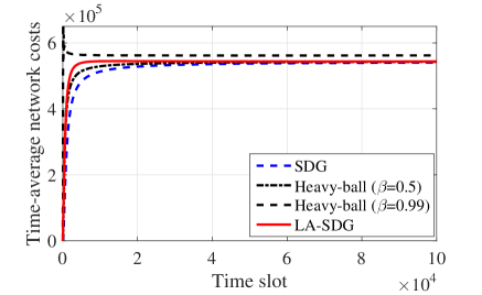
Figure 2: Comparison of time-averaged network costs.

Figure 3: Instantaneous queue lengths summed over all nodes.

VI Numerical Tests

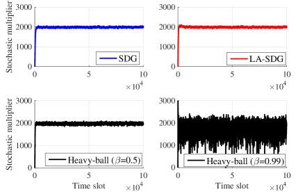
Figure 4: The evolution of stochastic multipliers at mapping node 1 ($\mu=0.2$).

This section presents numerical tests to confirm the analytical claims and demonstrate the merits of the proposed approach. We consider the geographical load balancing network of Section II-B with $K=10$ data centers, and $J=10$ mapping nodes. Performance is tested in terms of the time-averaged instantaneous network cost in (4), namely

$$\Psi_{t}(\mathbf{x}_{t})\!:=\sum_{k\in{\cal K}}p_{t}^{k}\left((x_{t}^{k0})^{2}-e_{t}^{k}\right)+\sum_{j\in{\cal J}}\sum_{k\in{\cal K}}b_{t}^{jk}(x_{t}^{jk})^{2}$$ (34)

where the energy price $p_{t}^{k}$ is uniformly distributed over $[10,30]$; samples of the renewable supply $\{e_{t}^{k}\}$ are generated uniformly over $[10,100]$; and the per-unit bandwidth cost is set to $b_{t}^{jk}=40/\bar{x}^{jk},\forall k,j$, with bandwidth limits $\{\bar{x}^{jk}\}$ generated from a uniform distribution within $[100,200]$. The capacities at data centers $\{\bar{x}_{t}^{k0}\}$ are uniformly generated from $[100,200]$. The delay-tolerant workloads $\{c_{t}^{j}\}$ arrive at each mapping node $j$ according to a uniform distribution over $[10,100]$. Clearly, the cost (34) and the state $\mathbf{s}_{t}$ here satisfy Assumptions 1 and 2. Finally, the stepsize is $\eta_{t}=1/\sqrt{t},\forall t$, the trade-off variable is $\mu=0.2$, and the bias correction vector is chosen as $\bm{\theta}=100\sqrt{\mu}\log^{2}(\mu)\bm{1}$ by default, but manually tuned in Figs. 5-6. We introduce two benchmarks: SDG in (13a) (see e.g., [4]), and the projected stochastic heavy-ball in (19) and $\beta=0.5$ by default (see e.g., [10]). Unless otherwise stated, all simulated results were averaged over 50 Monte Carlo realizations.

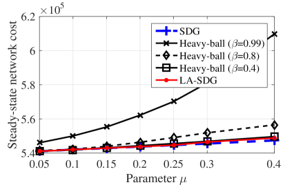
Figure 5: Comparison of steady-state network costs (after $10^{6}$ slots).

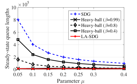
Figure 6: Steady-state queue lengths summed over all nodes (after $10^{6}$ slots).

Performance is first compared in terms of the time-averaged cost, and the instantaneous queue length in Figs. 2 and 3. For the network cost, SDG, LA-SDG, and the heavy-ball iteration with $\beta=0.5$ converge to almost the same value, while the heavy-ball method with a larger momentum factor $\beta=0.99$ exhibits a pronounced optimality loss. LA-SDG and heavy-ball exhibit faster convergence than SDG as their running-average costs quickly arrive at the optimal operating phase by leveraging the learning process or the momentum acceleration. In this test, LA-SDG exhibits a much lower delay as its aggregated queue length is only 10% of that for the heavy-ball method with $\beta=0.5$ and 4% of that for SDG. By using a larger $\beta$, the heavy-ball method incurs a much lower queue length relative to that of SDG, but still slightly higher than that of LA-SDG. Clearly, our learn-and-adapt procedure improves the delay performance.

Recall that the instantaneous resource allocation can be viewed as a function of the dual variable; see Proposition 1. Hence, the performance differences in Figs. 2-3 can be also anticipated by the different behavior of dual variables. In Fig. 4, the evolution of stochastic dual variables is plotted for a single Monte Carlo realization; that is the dual iterate in (13a) for SDG, the momentum iteration in (19) for the heavy-ball method, and the effective multiplier in (17b) for LA-SDG. As illustrated in (IV-B), the performance of momentum iterations is similar to SDG with larger stepsize ${\mu}/(1-\beta)$. This is corroborated by Fig. 4, where the stochastic momentum iterate with $\beta=0.5$ behaves similar to the dual iterates of SDG and LA-SDG, but its oscillation becomes prohibitively high with a larger factor $\beta=0.99$, which nicely explains the higher cost in Fig. 2.

Since the cost-delay performance is sensitive to the choice of parameters $\mu$ and $\beta$, extensive experiments are further conducted among three algorithms using different values of $\mu$ and $\beta$ in Figs. 5 and 6. The steady-state performance is evaluated by running algorithms for sufficiently long time, up to $10^{6}$ slots. The steady-state costs of all three algorithms increase as $\mu$ becomes larger, and the costs of LA-SDG and the heavy-ball with small momentum factor $\beta=0.4$ are close to that of SDG, while the costs of the heavy-ball with larger momentum factors $\beta=0.8$ and $\beta=0.99$ are much larger than that of SDG. Considering steady-state queue lengths (network delay), LA-SDG exhibits an order of magnitude lower amount than those of SDG and the heavy-ball with small $\beta$, under all choices of $\mu$. Note that the heavy-ball with a sufficiently large factor $\beta=0.99$ also has a very low queue length, but it incurs a higher cost than LA-SDG in Fig. 5 due to higher steady-state oscillation in Fig. 4.

VII Concluding Remarks

Fast convergent resource allocation and low service delay are highly desirable attributes of stochastic network management approaches. Leveraging recent advances in online learning and momentum-based optimization, a novel online approach termed LA-SDG was developed in this paper. LA-SDG learns the network state statistics through an additional sample recourse procedure. The associated novel iteration can be nicely interpreted as a modified heavy-ball recursion with an extra correction step to mitigate steady-state oscillations. It was analytically established that LA-SDG achieves a near-optimal cost-delay tradeoff $[\mu,\log^{2}(\mu)/\sqrt{\mu}]$, which is better than $[\mu,1/\mu]$ of SDG, at the cost of only one extra gradient evaluation per new datum. Our future research agenda includes novel approaches to further hedge against non-stationarity, and improved learning schemes to uncover other valuable statistical patterns from historical data.

Let us first state a simple but useful property regarding the primal-dual problems (7) and (11).

Proposition 3.

Under Assumptions 1-3, for the constrained optimization (7) with the optimal policy $\bm{\chi}^{*}(\cdot)$ and its optimal Lagrange multiplier $\bm{\lambda}^{*}$, it holds that $\mathbb{E}[\mathbf{A}\mathbf{x}_{t}^{*}+\mathbf{c}_{t}]=\mathbf{0}$ with $\mathbf{x}_{t}^{*}=\bm{\chi}^{*}(\mathbf{s}_{t})\in{\cal X}$, and accordingly that $\nabla{\cal D}(\bm{\lambda}^{*})=\mathbf{0}$.

Proof.

With $\bm{\lambda}^{*}$ denoting the optimal Lagrange multiplier with (7b), the Karush-Kuhn-Tucker (KKT) conditions [21] are

$$\left(\mathbb{E}[\nabla\Psi_{t}(\mathbf{x}_{t}^{*})]+\mathbf{A}^{\top}\bm{\lambda}^{*}\right)^{\top}(\mathbb{E}[\mathbf{x}_{t}-\mathbf{x}_{t}^{*}]) \geq 0,\;\forall\mathbf{x}_{t}\in{\cal X}$$ (35a)

$$(\bm{\lambda}^{*})^{\top}\mathbb{E}[\mathbf{A}\mathbf{x}_{t}^{*}+\mathbf{c}_{t}] =0$$ (35b)

$$\mathbb{E}[\mathbf{A}\mathbf{x}_{t}^{*}+\mathbf{c}_{t}]\leq\mathbf{0};\;\bm{\lambda}^{*} \geq\mathbf{0}$$ (35c)

where (35a) is the optimality condition of Lagrangian minimization, (35b) is the complementary slackness condition, and (35c) are the primal and dual feasibility conditions.

To establish the claim, let us first assume that there exists entry $k$ that the inequality constraint (7b) is not active; i.e., $\mathbb{E}[\mathbf{A}_{(k,:)}\mathbf{x}_{t}^{*}\!+\!c_{t}^{k}]=-\zeta$ with the constant $\zeta>0$, and $\mathbf{A}_{(k,:)}$ denoting the $k$-th row of $\mathbf{A}$. As each row of $\mathbf{A}$ has at least one entry equal to $-1$, we collect all indices of entries at $k$-th row with value $-1$ in set ${\cal E}_{k}^{-1}$ so that $\mathbf{A}_{(k,e)}=-1,\forall e\in{\cal E}_{k}^{-1}$.

Since $\mathbf{x}^{*}_{t}$ is feasible, we have $\mathbf{x}^{*}_{t}\geq\mathbf{0}$, and thus

$$\mathbb{E}[\mathbf{A}_{(k,:)}\mathbf{x}_{t}^{*}+c_{t}^{k}]=\mathbb{E}\left[\sum_{e\in{\cal E}}\mathbf{A}_{(k,e)}(x_{t}^{e})^{*}+c_{t}^{k}\right]=-\zeta$$ (36)

which implies that

$$\!\mathbb{E}\big{[}\textstyle\sum_{e\in{\cal E}_{k}^{-1}}(x_{t}^{e})^{*}\big{]}\!=\!\zeta+\mathbb{E}[c_{t}^{k}\!+\!\textstyle\sum_{e\in{\cal E}\backslash{\cal E}_{k}^{-1}}\mathbf{A}_{(k,e)}(x_{t}^{e})^{*}]>0.\!\!\!$$ (37)

According (35b), it further follows that $(\lambda^{k})^{*}=0$ since $(\lambda^{k})^{*}\cdot\mathbb{E}[\mathbf{A}_{(k,:)}\mathbf{x}_{t}^{*}\!+\!c_{t}^{k}]=-(\lambda^{k})^{*}\cdot\zeta=0$. Now we are on track to show that it contradicts with (35a). Since $\mathbb{E}[\sum_{e\in{\cal E}_{k}^{-1}}(x_{t}^{e})^{*}]>0$, there exists at least an index $j$ such that $\mathbb{E}[(x_{t}^{j})^{*}]>0,\,j\in{\cal E}_{k}^{-1}$. Choose $\mathbb{E}[\mathbf{x}_{t}]$ with $\mathbb{E}[x_{t}^{\tilde{j}}]=\mathbb{E}[(x_{t}^{\tilde{j}})^{*}],\forall{\tilde{j}}\neq j$ and $\mathbb{E}[x_{t}^{j}]=0$, to have $\mathbb{E}[\mathbf{x}_{t}-\mathbf{x}_{t}^{*}]=[0,\ldots,-\mathbb{E}[(x_{t}^{j})^{*}],\ldots,0]^{\top}$. Recall that the feasible set ${\cal X}$ in (3d) contains only box constraints; i.e., ${\cal X}:=\{\mathbf{x}\,|\,\mathbf{0}\leq\mathbf{x}\leq\bar{\mathbf{x}}\}$, which implies that the above selection of $\mathbf{x}_{t}$ is feasible. Hence, we arrive at (with $\nabla_{j}\Psi_{t}(\mathbf{x}_{t}^{*})$ denoting $j$-th entry of gradient)

$$\left(\mathbb{E}[\nabla\Psi_{t}(\mathbf{x}_{t}^{*})]+\mathbf{A}^{\top}\bm{\lambda}^{*}\right)^{\top}\mathbb{E}[(\mathbf{x}_{t}-\mathbf{x}_{t}^{*})]$$

$$= -\mathbb{E}\Big{[}\nabla_{j}\Psi_{t}(\mathbf{x}_{t}^{*})(x_{t}^{j})^{*}-\sum_{i\in{\cal I}}(\lambda^{i})^{*}\mathbf{A}_{(i,j)}(x_{t}^{j})^{*}\Big{]}$$

$$\stackrel{{\scriptstyle(a)}}{{=}} \underbrace{-\mathbb{E}[\nabla_{j}\Psi_{t}(\mathbf{x}_{t}^{*})(x_{t}^{j})^{*}]}_{<0}-\!\!\sum_{i\in{\cal I}\backslash k}\underbrace{(\lambda^{i})^{*}\mathbf{A}_{(i,j)}\mathbb{E}[(x_{t}^{j})^{*}]}_{\geq 0}<0$$ (38)

where (a) uses $(\lambda^{k})^{*}=0$; the first bracket follows from Assumption 2 since $\nabla_{j}\Psi_{t}(\mathbf{x}_{t}^{*})$ is monotonically increasing and $\nabla_{j}\Psi_{t}(\mathbf{x}_{t}^{*})\geq 0$, thus for $\mathbb{E}[(x_{t}^{j})^{*}]>0$ it follows $\mathbb{E}[\nabla_{j}\Psi_{t}(\mathbf{x}_{t}^{*})]>0$; and the second bracket follows that $\bm{\lambda}^{*}\geq\mathbf{0}$ and each column of $\mathbf{A}$ has at most one $-1$ and $\mathbf{A}_{(k,j)}=-1$. The proof is then complete since (VII) contradicts (35a). ∎

-A Proof of Lemma 2

Proof of Lipschitz continuity: Under Assumption 2, the primal objective $\Psi_{t}(\mathbf{x}_{t})$ is $\sigma$-strongly convex, and the smooth constant of the dual function ${\cal D}_{t}(\bm{\lambda})$, or equivalently, the Lipschitz constant of gradient $\nabla{\cal D}_{t}(\bm{\lambda})$ directly follows from [9, Lemma II.2], which equals to $L_{\rm d}=\rho(\mathbf{A}^{\top}\mathbf{A})/\sigma$, with $\rho(\mathbf{A}^{\top}\mathbf{A})$ denoting the maximum eigenvalue of $\mathbf{A}^{\top}\mathbf{A}$. We omit the derivations of this result, and refer readers to that in [9].

Supporting lemmas for quadratic growth: To prove the quadratic growth property (27), we introduce an error bound, which describes the local property of the dual function ${\cal D}(\bm{\lambda})$.

Lemma 5.

[30, Lemma 2.3] Consider the dual function in (10) and the feasible set ${\cal X}$ in (3d) with only linear constraints. For any $\bm{\lambda}$ satisfying ${\cal D}(\bm{\lambda})>-\infty$ and $\|\nabla{\cal D}(\bm{\lambda})\|\leq\delta$, we have

$$\|\bm{\lambda}^{*}-\bm{\lambda}\|\leq\xi\|\nabla{\cal D}(\bm{\lambda})\|$$ (39)

where the scalar $\xi$ depends on the matrix $\mathbf{A}$ as well the constants $\sigma$, $L_{\rm p}$ and $L_{\rm d}$ introduced in Assumption 2.

Lemma 5 states a local error bound for the dual function ${\cal D}(\bm{\lambda})$. The error bound is “local” since it holds only for $\bm{\lambda}$ close enough to the optimum $\bm{\lambda}^{*}$, i.e., $\|\nabla{\cal D}(\bm{\lambda})\|\leq\delta$. Following the arguments in [30] however, if the dual iterate $\bm{\lambda}$ is artificially confined to a compact set $\bm{\Lambda}$ such that $\|\bm{\lambda}\|\leq D$ with $D$ denoting the radius of $\bm{\Lambda}$, then for the case $\|\nabla{\cal D}(\bm{\lambda})\|\geq\delta$, the ratio ${\|\bm{\lambda}^{*}-\bm{\lambda}\|}/{\|\nabla{\cal D}(\bm{\lambda})\|}\leq D/\delta$, which implies the existence of $\xi$ satisfying (39) for any $\bm{\lambda}\in\bm{\Lambda}$. Lemma 5 is important for establishing linear convergence rate without strong convexity [30]. Remarkably, we will show next that this error bound is also critical to characterize the steady-state behavior of our LA-SDG scheme.

Building upon Lemma 5, we next show that the ensemble dual function ${\cal D}(\bm{\lambda})$ also satisfies the so-termed Polyak-Lojasiewicz (PL) condition [31].

Lemma 6.

Under Assumption 2, the local error-bound in (39) implies the following PL condition, namely

$${\cal D}(\bm{\lambda}^{*})-{\cal D}(\bm{\lambda})\leq\frac{L_{\rm d}\xi^{2}}{2}\|\nabla{\cal D}(\bm{\lambda})\|^{2}$$ (40)

where $L_{\rm d}$ is the Lipschitz constant of the dual gradient and $\xi$ is as in (39).

Proof.

Using the $L_{\rm d}$-smoothness of the dual function ${\cal D}(\bm{\lambda})$, we have for any $\bm{\lambda}$ and $\bm{\varphi}\in\mathbb{R}^{I}_{+}$ that

$$\!{\cal D}(\bm{\varphi})\leq{\cal D}(\bm{\lambda})-\langle\nabla{\cal D}(\bm{\varphi}),\bm{\lambda}-\bm{\varphi}\rangle+\frac{L_{\rm d}}{2}\|\bm{\lambda}-\bm{\varphi}\|^{2}\!.$$ (41)

Choosing $\bm{\varphi}=\bm{\lambda}^{*}$, and using Proposition 3 such that $\nabla{\cal D}(\bm{\lambda}^{*})=\mathbf{0}$, we have

$$\!{\cal D}(\bm{\lambda}^{*})\!\leq\!{\cal D}(\bm{\lambda})+\!\frac{L_{\rm d}}{2}\|\bm{\lambda}-\bm{\lambda}^{*}\|^{2}\!\stackrel{{\scriptstyle(a)}}{{\leq}}{\cal D}(\bm{\lambda})\!+\!\frac{L_{\rm d}\xi^{2}}{2}\|\nabla{\cal D}(\bm{\lambda})\|^{2}\!\!\!$$ (42)

where inequality (a) uses the local error-bound in (39). ∎

Proof of quadratic growth: The proof follows the main steps of that in [31]. Building upon Lemma 6, we next prove Lemma 2. Define a function of the dual variable $\bm{\lambda}$ as $g(\bm{\lambda}):=\sqrt{{\cal D}(\bm{\lambda}^{*})-{\cal D}(\bm{\lambda})}$. With the PL condition in (40), and $\bm{\Lambda}^{*}$ denoting the set of optimal multipliers for (11), we have for any $\bm{\lambda}\notin\bm{\Lambda}^{*}$ that

$$\|\nabla g(\bm{\lambda})\|^{2}=\frac{\|\nabla{\cal D}(\bm{\lambda})\|^{2}}{{\cal D}(\bm{\lambda}^{*})-{\cal D}(\bm{\lambda})}\geq\frac{2}{L_{\rm d}\xi^{2}}$$ (43)

which implies that $\|\nabla g(\bm{\lambda})\|\geq\sqrt{2/(L_{\rm d}\xi^{2})}$.

For any $\bm{\lambda}_{0}\!\notin\!\bm{\Lambda}^{*}$, consider the following differential equation

$$\frac{\mathbf{d}\bm{\lambda}(\tau)}{\mathbf{d}\tau}=-\nabla g(\bm{\lambda}(t))$$ (44a)

$$\;\bm{\lambda}(\tau=0)=\bm{\lambda}_{0}$$ (44b)

which describes the continuous trajectory of $\{\bm{\lambda}(\tau)\}$ starting from $\bm{\lambda}_{0}$ along the direction of $-\nabla g(\bm{\lambda}(\tau))$. By using $\|\nabla g(\bm{\lambda})\|\geq\sqrt{2/(L_{\rm d}\xi^{2})}$, it follows that $\nabla g(\bm{\lambda})$ is bounded below; thus, the differential equation (44) guarantees that we sufficiently reduce the value of function $g(\bm{\lambda})$, and $\bm{\lambda}(\tau)$ will eventually reach $\bm{\Lambda}^{*}$.

In other words, there exists a time $T$ such that $\bm{\lambda}(T)\in\bm{\Lambda}^{*}$. Formally, for $\tau>T$, we have

$$g(\bm{\lambda}_{0}) -g(\bm{\lambda}_{\tau})=\int_{\bm{\lambda}_{\tau}}^{\bm{\lambda}_{0}}\left\langle\nabla g(\bm{\lambda}),\mathbf{d}\bm{\lambda}\right\rangle$$

$$=-\int_{\bm{\lambda}_{0}}^{\bm{\lambda}_{\tau}}\left\langle\nabla g(\bm{\lambda}),\mathbf{d}\bm{\lambda}\right\rangle=-\int_{0}^{T}\left\langle\nabla g(\bm{\lambda}),\frac{\mathbf{d}\bm{\lambda}(\tau)}{\mathbf{d}\tau}\right\rangle\mathbf{d}\tau$$

$$=\int_{0}^{T}\|\nabla g(\bm{\lambda}(\tau))\|^{2}\mathbf{d}\tau\geq\int_{0}^{T}\frac{2}{L_{\rm d}\xi^{2}}\mathbf{d}\tau=\frac{2T}{L_{\rm d}\xi^{2}}.$$ (45)

Since $g(\bm{\lambda})\geq 0,\;\forall\bm{\lambda}$, we have $T\leq g(\bm{\lambda}_{0})L_{\rm d}\xi^{2}/2$, which implies that there exists a finite time $T$ such that $\bm{\lambda}_{\tau}\in\bm{\Lambda}^{*}$. On the other hand, the path length of trajectory $\{\bm{\lambda}(\tau)\}$ will be longer than the projection distance between $\bm{\lambda_{0}}$ and the closest point in $\bm{\Lambda}^{*}$ denoted as $\bm{\lambda}^{*}$, that is,

$$\int_{0}^{T}\left\|\frac{\mathbf{d}\bm{\lambda}(\tau)}{\mathbf{d}\tau}\right\|\mathbf{d}\tau=\int_{0}^{T}\left\|\nabla g(\bm{\lambda}(\tau))\right\|\mathbf{d}\tau\geq\|\bm{\lambda_{0}}-\bm{\lambda}^{*}\|$$ (46)

and thus we have from (-A) that

$$g(\bm{\lambda}_{0}) -g(\bm{\lambda}_{\tau})=\int_{0}^{T}\|\nabla g(\bm{\lambda}(\tau))\|^{2}\mathbf{d}\tau$$ (47)

$$\geq\int_{0}^{T}\|\nabla g(\bm{\lambda}(\tau))\|\sqrt{\frac{2}{L_{\rm d}\xi^{2}}}\mathbf{d}\tau\stackrel{{\scriptstyle(b)}}{{\geq}}\sqrt{\frac{2}{L_{\rm d}\xi^{2}}}\|\bm{\lambda_{0}}-\bm{\lambda}^{*}\|$$

where (b) follows from (46). Choosing $T$ such that $g(\bm{\lambda}_{T})=0$, we have

$$g(\bm{\lambda}_{0})\geq\sqrt{\frac{2}{L_{\rm d}\xi^{2}}}\|\bm{\lambda_{0}}-\bm{\lambda}^{*}\|.$$ (48)

Squaring both sides of (48), the proof is complete, since $\epsilon$ is defined as $\epsilon:=2/(L_{\rm d}\xi^{2})$ and $\bm{\lambda_{0}}$ can be any point outside the set of optimal multipliers.

-B Proof of Lemma 4

Since $\hat{\bm{\lambda}}_{t}$ converges to $\bm{\lambda}^{*},\;{\rm w.p.1}$ according to Theorem 1, there exists a finite time $T_{\theta}$ such that for $t>T_{\theta}$, we have $\|\bm{\lambda}^{*}-\hat{\bm{\lambda}}_{t}\|\leq\|\bm{\theta}\|$. In such case, it follows that $\tilde{\bm{\theta}}_{t}=\bm{\lambda}^{*}-\hat{\bm{\lambda}}_{t}+\bm{\theta}\geq\mathbf{0}$, since $\bm{\theta}\geq\mathbf{0}$. Therefore, we have

$$\|\mathbf{q}_{t+1}- \tilde{\bm{\theta}}_{t}/\mu\|^{2}=\|[\mathbf{q}_{t}+\mathbf{A}\mathbf{x}_{t}+\mathbf{c}_{t}]^{+}-[\tilde{\bm{\theta}}_{t}/\mu]^{+}\|^{2}$$ (49)

$$\stackrel{{\scriptstyle(a)}}{{\leq}} \|\mathbf{q}_{t}+\mathbf{A}\mathbf{x}_{t}+\mathbf{c}_{t}-\tilde{\bm{\theta}}_{t}/\mu\|^{2}$$

$$\stackrel{{\scriptstyle(b)}}{{\leq}} \|\mathbf{q}_{t}-\tilde{\bm{\theta}}_{t}/\mu\|^{2}+2(\mathbf{q}_{t}-\tilde{\bm{\theta}}_{t}/\mu)^{\top}(\mathbf{A}\mathbf{x}_{t}+\mathbf{c}_{t})+M^{2}$$

where (a) comes from the non-expansive property of the projection, and (b) is due to the bound $M$ in Assumption 4.

The RHS of (49) can be upper bounded by

$$\|\mathbf{q}_{t}-\tilde{\bm{\theta}}_{t}/\mu\|^{2}+2(\mathbf{q}_{t}-\tilde{\bm{\theta}}_{t}/\mu)^{\top}(\mathbf{A}\mathbf{x}_{t}+\mathbf{c}_{t})+M^{2}$$

$$\stackrel{{\scriptstyle(c)}}{{=}} \|\mathbf{q}_{t}-\tilde{\bm{\theta}}_{t}/\mu\|^{2}+\frac{2}{\mu}\left(\bm{\gamma}_{t}-\bm{\lambda}^{*}\right)^{\top}(\mathbf{A}\mathbf{x}_{t}+\mathbf{c}_{t})+M^{2}$$ (50)

where (c) uses the definitions $\tilde{\bm{\theta}}_{t}:=\bm{\lambda}^{*}-\hat{\bm{\lambda}}_{t}+\bm{\theta}$, and $\bm{\gamma}_{t}:=\hat{\bm{\lambda}}_{t}+\mu\mathbf{q}_{t}-\bm{\theta}$. Since $\mathbf{A}\mathbf{x}_{t}+\mathbf{c}_{t}$ is the stochastic subgradient of the concave function ${\cal D}(\bm{\lambda})$ at $\bm{\lambda}=\bm{\gamma}_{t}$ [cf. (17a)], we have

$$\mathbb{E}\left[\left(\bm{\gamma}_{t}-\bm{\lambda}^{*}\right)^{\top}(\mathbf{A}\mathbf{x}_{t}+\mathbf{c}_{t})\right]\leq{\cal D}(\bm{\gamma}_{t})-{\cal D}(\bm{\lambda}^{*}).$$ (51)

Taking expectations on (49)-(-B) over the random state $\mathbf{s}_{t}$ conditioned on $\mathbf{q}_{t}$ and using (51), we arrive at

$$\mathbb{E}\left[\|\mathbf{q}_{t+1}\!-\!\tilde{\bm{\theta}}_{t}/\mu\|^{2}\right]\!\leq\!\|\mathbf{q}_{t}-\tilde{\bm{\theta}}_{t}/\mu\|^{2}\!+\frac{2}{\mu}\left({\cal D}(\bm{\gamma}_{t})-{\cal D}(\bm{\lambda}^{*})\right)+M^{2}$$ (52)

where we use the fact that ${\cal D}(\bm{\lambda}):=\mathbb{E}\left[{\cal D}_{t}(\bm{\lambda})\right]$ in (11). Using the quadratic growth property of ${\cal D}(\bm{\lambda})$ in (27) of Lemma 2, the recursion (52) further leads to

$$\mathbb{E}\big{[}\|\mathbf{q}_{t+1}- \tilde{\bm{\theta}}_{t}/\mu\|^{2}\big{]}\leq\|\mathbf{q}_{t}-\tilde{\bm{\theta}}_{t}/\mu\|^{2}\!-\frac{2\epsilon}{\mu}\|\bm{\gamma}_{t}-\bm{\lambda}^{*}\|^{2}+M^{2}$$

$$\stackrel{{\scriptstyle(d)}}{{=}} \|\mathbf{q}_{t}-\tilde{\bm{\theta}}_{t}/\mu\|^{2}-2\mu\epsilon\|\mathbf{q}_{t}-\tilde{\bm{\theta}}_{t}/\mu\|^{2}+M^{2}$$ (53)

where equality (d) uses the definitions $\tilde{\bm{\theta}}_{t}:=\bm{\lambda}^{*}-\hat{\bm{\lambda}}_{t}+\bm{\theta}$ and $\bm{\gamma}_{t}:=\hat{\bm{\lambda}}_{t}+\mu\mathbf{q}_{t}-\bm{\theta}$, implying that $\bm{\gamma}_{t}-\bm{\lambda}^{*}=\mu\mathbf{q}_{t}-\tilde{\bm{\theta}}_{t}$.

Now considering (cf. (-B))

$$-2\mu\epsilon\|\mathbf{q}_{t}-\tilde{\bm{\theta}}_{t}/\mu\|^{2}+M^{2}\leq-2\sqrt{\mu}\|\mathbf{q}_{t}-\tilde{\bm{\theta}}_{t}/\mu\|+\mu$$ (54)

and plugging it back into (-B) yields

$$\mathbb{E}\big{[}\|\mathbf{q}_{t+1}-\tilde{\bm{\theta}}_{t}/\mu\|^{2}\big{]} \leq\|\mathbf{q}_{t}-\tilde{\bm{\theta}}_{t}/\mu\|^{2}-2\sqrt{\mu}\|\mathbf{q}_{t}-\tilde{\bm{\theta}}_{t}/\mu\|+\mu$$

$$=\big{(}\|\mathbf{q}_{t}-\tilde{\bm{\theta}}_{t}/\mu\|-\sqrt{\mu}\big{)}^{2}.$$ (55)

By the convexity of $(\,\cdot\,)^{2}$, we further arrive at

$$\mathbb{E}\left[\|\mathbf{q}_{t+1}-\tilde{\bm{\theta}}_{t}/\mu\|\right]^{2} \leq\mathbb{E}\big{[}\|\mathbf{q}_{t+1}-\tilde{\bm{\theta}}_{t}/\mu\|^{2}\big{]}$$

$$\leq\left(\|\mathbf{q}_{t}-\tilde{\bm{\theta}}_{t}/\mu\|-\sqrt{\mu}\right)^{2}$$ (56)

which directly implies the argument (31) in the lemma. By checking Vieta’s formulas for second-order equations, there exists $B=\Theta(\frac{1}{\sqrt{\mu}})$ such that for $\|\mathbf{q}_{t}-\tilde{\bm{\theta}}_{t}/\mu\|>B$, inequality (54) holds, and thus the lemma follows readily.

-C Proof of Theorem 2

Proof of (32a) in Theorem 2: Theorem 1 asserts that $\hat{\bm{\lambda}}_{t}$ eventually converges to the optimum $\bm{\lambda}^{*},\,{\rm w.p.1}$. Hence, there always exists a finite time $T_{\rho}$ and an arbitrarily small $\rho$ such that for $t>T_{\rho}$, it holds that $\|\bm{\lambda}^{*}/\mu-\hat{\bm{\lambda}}_{t}/\mu\|\leq\rho$. Using the definition $\tilde{\bm{\theta}}_{t}=\bm{\lambda}^{*}-\hat{\bm{\lambda}}_{t}+\bm{\theta}$, it then follows by the triangle inequality that

$$\left|\|\mathbf{q}_{t}-\tilde{\bm{\theta}}_{t}/\mu\|-\|\mathbf{q}_{t}-\bm{\theta}/\mu\|\right|\leq\|\bm{\lambda}^{*}/\mu-\hat{\bm{\lambda}}_{t}/\mu\|\leq\rho$$ (57)

which also holds for $\mathbf{q}_{t+1}$.

Using (57) and the conditional drift (31) in Lemma 4, for $t\!>\!T_{\rho}$ and $\|\mathbf{q}_{t}-\tilde{\bm{\theta}}_{t}/\mu\|\!>\!B\!=\!\Theta({1}/{\sqrt{\mu}})$, it holds that

$$\mathbb{E}\left[\left\|\mathbf{q}_{t+1}-\bm{\theta}/\mu\right\|\Big{|}\mathbf{q}_{t}\right]\leq\mathbb{E}\left[\left\|\mathbf{q}_{t+1}-\tilde{\bm{\theta}}_{t}/\mu\right\|\Big{|}\mathbf{q}_{t}\right]+\rho$$

$$\leq \left\|\mathbf{q}_{t}-\tilde{\bm{\theta}}_{t}/\mu\right\|-\sqrt{\mu}+\rho\leq\left\|\mathbf{q}_{t}-\bm{\theta}/\mu\right\|-\sqrt{\mu}+2\rho.$$ (58)

Choosing $\rho$ such that $\sqrt{\tilde{\mu}}:=\sqrt{\mu}-2\rho<0$, then for $t\!>\!T_{\rho}$ and $\|\mathbf{q}_{t}-\bm{\theta}/\mu\|\!>\tilde{B}\!:=\!B+\rho\!=\!\Theta({1}/{\sqrt{\mu}})$, we have

$$\mathbb{E}\left[\left\|\mathbf{q}_{t+1}-\bm{\theta}/\mu\right\|\Big{|}\mathbf{q}_{t}\right]\leq\left\|\mathbf{q}_{t}-\bm{\theta}/\mu\right\|-\sqrt{\tilde{\mu}}.$$ (59)

Leveraging (59), we first show (32a) by constructing a super-martingale. Define the stochastic process $a_{t}$ as

$$a_{t}:=\left\|\mathbf{q}_{t}-\bm{\theta}/\mu\right\|\cdot\mathds{1}\left\{\min_{\tau\leq t}\left\|\mathbf{q}_{\tau}-\bm{\theta}/\mu\right\|>\tilde{B}\right\},\,\forall t$$ (60a)

and likewise the stochastic process $$b_{t}$$ as

$$b_{t}:=\sqrt{\tilde{\mu}}\cdot\mathds{1}\left\{\min_{\tau\leq t}\left\|\mathbf{q}_{\tau}-\bm{\theta}/\mu\right\|>\tilde{B}\right\},\;\forall t.$$ (60b)

Clearly, $a_{t}$ tracks the distance between $\mathbf{q}_{t}$ and $\bm{\theta}/\mu$ until the distance becomes smaller than $\tilde{B}$ for the first time; and $b_{t}$ stops until $\left\|\mathbf{q}_{t}-\bm{\theta}/\mu\right\|\leq\tilde{B}$ for the first time as well.

With the definitions of $a_{t}$ and $b_{t}$, one can easily show that the recursion (59) implies

$$\mathbb{E}\left[a_{t+1}|\mathbf{\cal F}_{t}\right]\leq a_{t}-b_{t}$$ (61)

where $\mathbf{\cal F}_{t}$ is the so-termed sigma algebra measuring the history of two processes. As $a_{t}$ and $b_{t}$ are both nonnegative, (61) allows us to apply the super-martingale convergence theorem [23, Theorem E7.4], which almost surely establishes that: (i) the sequence $a_{t}$ converges to a limit; and (ii) the summation $\sum_{t=1}^{\infty}b_{t}<\infty$. Note that (ii) implies that $\lim_{t\rightarrow\infty}b_{t}=0$, ${\rm w.p.1}$. Since $\sqrt{\tilde{\mu}}>0$, it follows that the indicator function of $b_{t}$ eventually becomes null and thus

$$\liminf_{t\rightarrow\infty}\;\;\left\|\mathbf{q}_{t}-\bm{\theta}/\mu\right\|\leq\tilde{B},\;\;{\rm w.p.1}$$ (62)

which establishes that $\mathbf{q}_{t}$ will eventually visit and then hover around a neighborhood of the reference point $\bm{\theta}/\mu$.

Proof of (32b) in Theorem 2: In complement to the sample-path result in (62), we next derive (32b), which captures the long-term queue lengths averaged over all sample paths.

Similar to (49), we have

$$\|\mathbf{q}_{t+1}-\bm{\lambda}^{*}/\mu\|^{2}\leq$$ (63)

$$\qquad\qquad\|\mathbf{q}_{t}-\bm{\lambda}^{*}/\mu\|^{2}+2(\mathbf{q}_{t}-\bm{\lambda}^{*}/\mu)^{\top}(\mathbf{A}\mathbf{x}_{t}+\mathbf{c}_{t})+M^{2}.$$

Using the definition $\bm{\gamma}_{t}:=\hat{\bm{\lambda}}_{t}+\mu\mathbf{q}_{t}-\bm{\theta}$, (64) can be written as

$$\|\mathbf{q}_{t+1}-\bm{\lambda}^{*}/\mu\|^{2}\leq\|\mathbf{q}_{t}-\bm{\lambda}^{*}/\mu\|^{2}$$ (64)

$$+\frac{2}{\mu}(\bm{\gamma}_{t}-\bm{\lambda}^{*})^{\top}(\mathbf{A}\mathbf{x}_{t}+\mathbf{c}_{t})+\frac{2}{\mu}(\bm{\theta}-\hat{\bm{\lambda}}_{t})^{\top}(\mathbf{A}\mathbf{x}_{t}+\mathbf{c}_{t})+M^{2}.$$

Defining the Lyapunov drift as $\Delta(\mathbf{q}_{t})\!:=\!\frac{1}{2}(\|\mathbf{q}_{t+1}-\bm{\lambda}^{*}/\mu\|^{2}\!-\!\|\mathbf{q}_{t}-\bm{\lambda}^{*}/\mu\|^{2})$ and taking expectations on (64) over $\mathbf{s}_{t}$ conditioned on $\mathbf{q}_{t}$, we have

$$\mu\mathbb{E}\left[\Delta(\mathbf{q}_{t})\right]\leq\mathbb{E}\Big{[}(\bm{\gamma}_{t}-\bm{\lambda}^{*})^{\!\top}\!(\mathbf{A}\mathbf{x}_{t}\!+\!\mathbf{c}_{t})\Big{]}$$

$$\qquad\qquad\qquad\qquad~{}+\mathbb{E}\Big{[}(\bm{\theta}\!-\!\hat{\bm{\lambda}}_{t})^{\!\top}\!(\mathbf{A}\mathbf{x}_{t}+\mathbf{c}_{t})\Big{]}\!+\!{\mu M^{2}}/{2}$$

$$\stackrel{{\scriptstyle(b)}}{{\leq}}{\cal D}(\bm{\gamma}_{t})\!-\!{\cal D}(\bm{\lambda}^{*})\!+\mathbb{E}\Big{[}(\bm{\theta}\!-\!\hat{\bm{\lambda}}_{t})^{\!\top}\!(\mathbf{A}\mathbf{x}_{t}\!+\!\mathbf{c}_{t})\Big{]}\!+\!{\mu M^{2}}/{2}$$ (65)

where (b) follows from (51).

Summing both sides over $t=1,\ldots,T$, taking expectations over all possible $\mathbf{q}_{t}$, and dividing both sides by $T$, we arrive at

$$\frac{\mu}{2T}\left(\mathbb{E}\left[\|\mathbf{q}_{T+1}-\bm{\lambda}^{*}/\mu\|^{2}\right]-\mathbb{E}\left[\|\mathbf{q}_{1}-\bm{\lambda}^{*}/\mu\|^{2}\right]\right)\leq$$ (66)

$$\frac{1}{T}\!\sum_{t=1}^{T}\mathbb{E}[{\cal D}(\bm{\gamma}_{t})]\!-\!{\cal D}(\bm{\lambda}^{*})\!+\!\frac{1}{T}\!\sum_{t=1}^{T}\mathbb{E}\Big{[}(\bm{\theta}\!-\!\hat{\bm{\lambda}}_{t})^{\!\top}\!(\mathbf{A}\mathbf{x}_{t}\!+\!\mathbf{c}_{t})\Big{]}\!\!+\!\frac{\mu M^{2}}{2}.$$

First, it is easy to show that

$$\lim_{T\rightarrow\infty}\frac{\mu}{2T}\left(\mathbb{E}\left[\left\|\mathbf{q}_{T+1}-{\bm{\lambda}^{*}}/{\mu}\right\|^{2}\right]-\mathbb{E}\left[\left\|\mathbf{q}_{1}-{\bm{\lambda}^{*}}/{\mu}\right\|^{2}\right]\right)$$

$$\stackrel{{\scriptstyle(c)}}{{\geq}} -\lim_{T\rightarrow\infty}\frac{\mu}{2T}\mathbb{E}\left[\left\|\mathbf{q}_{1}-{\bm{\lambda}^{*}}/{\mu}\right\|^{2}\right]\stackrel{{\scriptstyle(d)}}{{=}}0$$ (67)

where (c) holds since $\left\|\mathbf{q}_{T+1}-{\bm{\lambda}^{*}}/{\mu}\right\|^{2}\geq 0$, and (d) follows from the boundedness of $\left\|\mathbf{q}_{1}-{\bm{\lambda}^{*}}/{\mu}\right\|^{2}$.

We next argue that the following equality holds

$$\lim_{T\rightarrow\infty}({1}/{T})\;\textstyle\sum_{t=1}^{T}\mathbb{E}\left[(\bm{\theta}-\hat{\bm{\lambda}}_{t})^{\top}(\mathbf{A}\mathbf{x}_{t}+\mathbf{c}_{t})\right]={\cal O}(\mu).$$ (68)

Rearranging terms in (68) leads to

$$\lim_{T\rightarrow\infty}\frac{1}{T}\sum_{t=1}^{T}\mathbb{E}\left[(\bm{\theta}-\hat{\bm{\lambda}}_{t})^{\top}(\mathbf{A}\mathbf{x}_{t}+\mathbf{c}_{t})\right]$$ (69)

$$= \lim_{T\rightarrow\infty}\frac{1}{T}\sum_{t=1}^{T}\mathbb{E}\left[\left(\bm{\theta}-\bm{\lambda}^{*}+(\bm{\lambda}^{*}\!-\!\bm{\theta}\!-\!\hat{\bm{\lambda}}_{t}\!+\!\bm{\theta})\right)^{\top}(\mathbf{A}\mathbf{x}_{t}+\mathbf{c}_{t})\right].$$

Since $\hat{\bm{\lambda}}_{t}$ converges to $\bm{\lambda}^{*}\,{\rm w.p.1}$ according to Theorem 1, there always exists a finite time $T_{\rho}$ such that for $t>T_{\rho}$, which implies that $\|\bm{\lambda}^{*}-\bm{\theta}-(\hat{\bm{\lambda}}_{t}-\bm{\theta})\|\leq\rho,\;{\rm w.p.1}$. Hence, together with the Cauchy-Schwarz inequality, we have

$$(\bm{\lambda}^{*}\!-\!\bm{\theta}\!-\!\hat{\bm{\lambda}}_{t}\!+\!\bm{\theta})^{\top}(\mathbf{A}\mathbf{x}_{t}+\mathbf{c}_{t})$$

$$\leq \|\bm{\lambda}^{*}\!-\!\bm{\theta}\!-\!(\hat{\bm{\lambda}}_{t}\!-\!\bm{\theta})\|\|\mathbf{A}\mathbf{x}_{t}\!+\!\mathbf{c}_{t}\|\stackrel{{\scriptstyle(d)}}{{\leq}}\rho M={\cal O}(\rho)$$ (70)

where (d) follows since $T_{\rho}\!<\!\infty$ and constant $M$ is as in Assumption 4. Plugging (-C) into (69), it follows that

$$\lim_{T\rightarrow\infty}({1}/{T})\textstyle\sum_{t=1}^{T}\mathbb{E}\left[(\bm{\theta}-\hat{\bm{\lambda}}_{t})^{\top}(\mathbf{A}\mathbf{x}_{t}+\mathbf{c}_{t})\right]$$ (71)

$$\leq \lim_{T\rightarrow\infty}({1}/{T})\;\textstyle\sum_{t=1}^{T}\mathbb{E}\left[(\bm{\theta}-\bm{\lambda}^{*})^{\top}(\mathbf{A}\mathbf{x}_{t}+\mathbf{c}_{t})\right]+{\cal O}(\rho)$$

$$\stackrel{{\scriptstyle(e)}}{{\leq}} \|\bm{\lambda}^{*}-\bm{\theta}\|\cdot\left\|\lim_{T\rightarrow\infty}({1}/{T})\;\textstyle\sum_{t=1}^{T}\mathbb{E}\left[-\mathbf{A}\mathbf{x}_{t}-\mathbf{c}_{t}\right]\right\|+{\cal O}(\rho)$$

where (e) simply follows from the Cauchy-Schwarz inequality.

Building upon (59), one can follow the arguments in [14, Theorem 4] to show that there exist constants $D_{1}\!=\!\Theta(1/\mu)$, and $D_{2}\!=\!\Theta(\sqrt{\mu})$, for any $d$, to obtain a large deviation bound as

$$\lim_{T\rightarrow\infty}\frac{1}{T}\sum_{t=1}^{T}\mathbb{P}\left(\|\mathbf{q}_{t}-\bm{\theta}/\mu\|>\tilde{B}+d\right)\leq D_{1}e^{-D_{2}d}$$ (72)

where $\tilde{B}=\!\Theta({1}/{\sqrt{\mu}})$ as in (59). Intuitively speaking, (72) upper bounds the probability that the steady-state $\mathbf{q}_{t}$ deviates from $\bm{\theta}/\mu$, and (72) implies that the probability that $q^{i}_{t}>\theta/\mu+\tilde{B}+d,\;\forall i$ is exponentially decreasing in $D_{2}d$.

Using the large deviation bound in (72), it follows that

$$\mathbf{0} \stackrel{{\scriptstyle(f)}}{{\leq}}\!\lim_{T\rightarrow\infty}\frac{1}{T}\sum_{t=1}^{T}\mathbb{E}[-\mathbf{A}\mathbf{x}_{t}-\mathbf{c}_{t}]$$ (73)

$$\stackrel{{\scriptstyle(g)}}{{\leq}}\!\lim_{T\rightarrow\infty}\frac{1}{T}\sum_{t=1}^{T}\mathbf{1}\!\cdot\!{M}\,\mathbb{P}\left(\mathbf{q}_{t}<M\right)\stackrel{{\scriptstyle(h)}}{{\leq}}\!\mathbf{1}\!\cdot\!MD_{1}e^{-D_{2}(\bm{\theta}/\mu-\tilde{B}-M)}$$

where (f) holds because taking expectation in (72) over all $d$ implies that the expected queue length is finite [cf. (3c)], which implies the necessary condition in (5); (g) follows from [15, Lemma 4] which establishes that negative accumulated service residual $\sum_{t=1}^{T}\mathbb{E}[\mathbf{A}\mathbf{x}_{t}+\mathbf{c}_{t}]$ may happen only when $\mathbf{q}_{t}\!<\!M$ and the maximum value is bounded by $\|\mathbf{A}\mathbf{x}_{t}+\mathbf{c}_{t}\|\leq M$ in Assumption 4; and (h) uses the bound in (72) by choosing $d=\bm{\theta}/\mu-\tilde{B}-M$.

Setting $\bm{\theta}=\sqrt{\mu}\log^{2}(\mu)$ in (73), there exists a sufficiently small $\mu$ such that $-D_{2}\big{(}\log^{2}(\mu)/\sqrt{\mu}-\tilde{B}-M\big{)}\leq 2\log(\mu)$. Together with (73) and $D_{1}\!=\!\Theta(1/\mu)$, the latter implies that

$$\left\|\lim_{T\rightarrow\infty}\!({1}/{T})\textstyle\sum_{t=1}^{T}\mathbb{E}[-\mathbf{A}\mathbf{x}_{t}\!-\!\mathbf{c}_{t}]\right\|\leq\|\mathbf{1}\cdot MD_{1}\mu^{2}\|={\cal O}(\mu).$$ (74)

Plugging (74) into (71), setting $\rho=\mathbf{o}(\mu)$ in (71), and using $\|\bm{\lambda}^{*}-\bm{\theta}\|={\cal O}(1)$, we arrive at (68).

Letting $T\rightarrow\infty$ in (66), it follows from (-C) and (68) that

$$0 \leq\lim_{T\rightarrow\infty}\frac{1}{T}\!\sum_{t=1}^{T}\mathbb{E}[{\cal D}(\bm{\gamma}_{t})]\!-\!{\cal D}(\bm{\lambda}^{*})\!+{\cal O}(\mu)+\!\frac{\mu M^{2}}{2}$$

$$\stackrel{{\scriptstyle(h)}}{{\leq}}{\cal D}\left(\lim_{T\rightarrow\infty}\frac{1}{T}\!\sum_{t=1}^{T}\mathbb{E}[\bm{\gamma}_{t}]\right)\!-\!{\cal D}(\bm{\lambda}^{*})\!+{\cal O}(\mu)+\!\frac{\mu M^{2}}{2}.$$ (75)

where inequality (h) uses the concavity of the dual function ${\cal D}(\bm{\lambda})$. Defining $\bm{\varphi}:=\lim_{T\rightarrow\infty}\frac{1}{T}\!\sum_{t=1}^{T}\mathbb{E}[\bm{\gamma}_{t}]$, and using ${\cal D}(\bm{\lambda}^{*})-{\cal D}(\bm{\varphi})\geq\frac{\epsilon}{2}\|\bm{\lambda}^{*}-\bm{\varphi}\|^{2}$ in Lemma 2, (-C) implies that

$$\|\bm{\lambda}^{*}-\bm{\varphi}\|^{2}\!\leq\!\frac{2}{\epsilon}\Big{(}{\cal D}(\bm{\lambda}^{*})-{\cal D}(\bm{\varphi})\Big{)}\!\leq\!{\cal O}(\mu)+\frac{\mu M^{2}}{\epsilon}\!\stackrel{{\scriptstyle(i)}}{{=}}\!{\cal O}(\mu)\!$$ (76)

where (i) follows since constants $M$ and $\epsilon$ are independent of $\mu$. From (76), we can further conclude that $\|\bm{\lambda}^{*}-\bm{\varphi}\|={\cal O}(\sqrt{\mu})$.

Recalling the definition $\bm{\gamma}_{t}:=\hat{\bm{\lambda}}_{t}+\mu\mathbf{q}_{t}-\bm{\theta}$, we have that

$$\lim_{T\rightarrow\infty}\!\frac{1}{T}\!\sum_{t=1}^{T}\mathbb{E}\!\left[\frac{\bm{\gamma}_{t}}{\mu}\right]\!-\!\frac{\bm{\lambda}^{*}}{\mu}\!=\!\lim_{T\rightarrow\infty}\!\frac{1}{T}\!\sum_{t=1}^{T}\mathbb{E}\!\left[\mathbf{q}_{t}\!+\!\frac{\hat{\bm{\lambda}}_{t}}{\mu}\right]\!-\!\frac{\bm{\lambda}^{*}}{\mu}\!-\!\frac{\bm{\theta}}{\mu}$$

$$\stackrel{{\scriptstyle(j)}}{{=}} \lim_{T\rightarrow\infty}\frac{1}{T}\!\sum_{t=1}^{T}\mathbb{E}\left[\mathbf{q}_{t}\right]\!-\!\frac{\bm{\theta}}{\mu}\stackrel{{\scriptstyle(k)}}{{\leq}}\frac{1}{\mu}\|\bm{\lambda}^{*}-\bm{\varphi}\|={\cal O}\left(\frac{1}{\sqrt{\mu}}\right)$$ (77)

where (j) follows from the convergence of $\hat{\bm{\lambda}}_{t}$ in Theorem 1, and inequality (k) uses the definition of $\bm{\varphi}$ and $\bm{\varphi}-\bm{\lambda}^{*}\leq\|\bm{\lambda}^{*}-\bm{\varphi}\|$. Recalling that $\bm{\theta}=\sqrt{\mu}\log^{2}(\mu)$ in (74) completes the proof.

-D Proof of Theorem 3

Defining the Lyapunov drift as $\Delta(\mathbf{q}_{t})\!:=\!\frac{1}{2}(\|\mathbf{q}_{t+1}\|^{2}\!-\!\|\mathbf{q}_{t}\|^{2})$, and squaring the queue update, we obtain

$$\|\mathbf{q}_{t+1}\|^{2}= \|\mathbf{q}_{t}\|^{2}+2\mathbf{q}_{t}^{\top}(\mathbf{A}\mathbf{x}_{t}+\mathbf{c}_{t})+\|\mathbf{A}\mathbf{x}_{t}+\mathbf{c}_{t}\|^{2}$$

$$\stackrel{{\scriptstyle(a)}}{{\leq}} \|\mathbf{q}_{t}\|^{2}+2\mathbf{q}_{t}^{\top}(\mathbf{A}\mathbf{x}_{t}+\mathbf{c}_{t})+M^{2}$$ (78)

where (a) follows from the definition of $M$ in Assumption 4. Multiplying by $\mu/2$ and adding $\Psi_{t}(\mathbf{x}_{t})$, yields

$$\mu\Delta(\mathbf{q}_{t})+ \Psi_{t}(\mathbf{x}_{t})\leq\Psi_{t}(\mathbf{x}_{t})+\mu\mathbf{q}_{t}^{\top}(\mathbf{A}\mathbf{x}_{t}+\mathbf{c}_{t})+{\mu M^{2}}/{2}$$

$$\stackrel{{\scriptstyle(b)}}{{=}} \Psi_{t}(\mathbf{x}_{t})+(\bm{\gamma}_{t}-\hat{\bm{\lambda}}_{t}+\bm{\theta})^{\top}(\mathbf{A}\mathbf{x}_{t}+\mathbf{c}_{t})+{\mu M^{2}}/{2}$$

$$\stackrel{{\scriptstyle(c)}}{{=}} {\cal L}_{t}(\mathbf{x}_{t},\bm{\gamma}_{t})+(\bm{\theta}-\hat{\bm{\lambda}}_{t})^{\top}(\mathbf{A}\mathbf{x}_{t}+\mathbf{c}_{t})+{\mu M^{2}}/{2}$$ (79)

where (b) uses the definition of $\bm{\gamma}_{t}$, and (c) is the definition of the instantaneous Lagrangian. Taking expectations on the both sides of (-D) over $\mathbf{s}_{t}$ conditioned on $\mathbf{q}_{t}$, it holds that

$$\mu\mathbb{E}\left[\Delta(\mathbf{q}_{t})\big{|}\mathbf{q}_{t}\right]+\mathbb{E}\left[\Psi_{t}(\mathbf{x}_{t})\big{|}\mathbf{q}_{t}\right]$$

$$\stackrel{{\scriptstyle(d)}}{{=}} {\cal D}(\bm{\gamma}_{t})+\mathbb{E}\left[(\bm{\theta}-\hat{\bm{\lambda}}_{t})^{\top}(\mathbf{A}\mathbf{x}_{t}+\mathbf{c}_{t})\big{|}\mathbf{q}_{t}\right]+{\mu M^{2}}/{2}$$

$$\stackrel{{\scriptstyle(e)}}{{\leq}} {\Psi}^{*}+\mathbb{E}\left[(\bm{\theta}-\hat{\bm{\lambda}}_{t})^{\top}(\mathbf{A}\mathbf{x}_{t}+\mathbf{c}_{t})\big{|}\mathbf{q}_{t}\right]+{\mu M^{2}}/{2}$$ (80)

where (d) follows from the definition of the dual function (10), while (e) uses the weak duality that ${\cal D}(\bm{\gamma}_{t})\leq\tilde{\Psi}^{*}$, and the fact that $\tilde{\Psi}^{*}\leq{\Psi}^{*}$ (cf. the discussion after (6)).

Taking expectations on both sides of (-D) over all possible $\mathbf{q}_{t}$, summing over $t=1,\ldots,T$, dividing by $T$, and letting $T\rightarrow\infty$, we arrive at

$$\lim_{T\rightarrow\infty}\frac{1}{T}\sum_{t=1}^{T}\mathbb{E}\left[\Psi_{t}(\mathbf{x}_{t})\right]$$

$$\!\!\!\stackrel{{\scriptstyle(f)}}{{\leq}} {\Psi}^{*}\!\!+\!\!\lim_{T\rightarrow\infty}\!\frac{1}{T}{\sum_{t=1}^{T}\mathbb{E}\!\left[(\bm{\theta}\!-\!\hat{\bm{\lambda}}_{t})\!^{\top}\!(\mathbf{A}\mathbf{x}_{t}\!+\!\mathbf{c}_{t})\right]}\!\!+\!\frac{\mu M^{2}}{2}\!+\!\!\lim_{T\rightarrow\infty}\!\!\!\frac{\mu\|\mathbf{q}_{1}\|^{2}}{2T}$$

$$\!\!\!\stackrel{{\scriptstyle(g)}}{{\leq}} {\Psi}^{*}\!+\!\lim_{T\rightarrow\infty}\frac{1}{T}{\sum_{t=1}^{T}\mathbb{E}\left[(\bm{\theta}-\hat{\bm{\lambda}}_{t})^{\top}(\mathbf{A}\mathbf{x}_{t}+\mathbf{c}_{t})\right]}\!+\!\frac{\mu M^{2}}{2}\!$$ (81)

where (f) comes from $\mathbb{E}[\|\mathbf{q}_{T+1}\|^{2}]\geq 0$, and (g) follows because $\|\mathbf{q}_{1}\|$ is bounded. One can follow the derivations in (69)-(74) to show (68), which is the second term in the RHS of (-D). Therefore, we have from (-D) that

$$\lim_{T\rightarrow\infty}\frac{1}{T}\sum_{t=1}^{T}\mathbb{E}\left[\Psi_{t}(\mathbf{x}_{t})\right] \leq{\Psi}^{*}\!+\!{\cal O}(\mu)+\frac{\mu M^{2}}{2}$$ (82)

which completes the proof.

References

- [1] L. Tassiulas and A. Ephremides, “Stability properties of constrained queueing systems and scheduling policies for maximum throughput in multihop radio networks,” IEEE Trans. Automat. Contr., vol. 37, no. 12, pp. 1936–1948, Dec. 1992.
- [2] S. H. Low and D. E. Lapsley, “Optimization flow control-I: basic algorithm and convergence,” IEEE/ACM Trans. Networking, vol. 7, no. 6, pp. 861–874, Dec. 1999.
- [3] L. Georgiadis, M. Neely, and L. Tassiulas, “Resource allocation and cross-layer control in wireless networks,” Found. and Trends in Networking, vol. 1, pp. 1–144, 2006.
- [4] M. J. Neely, “Stochastic network optimization with application to communication and queueing systems,” Synthesis Lectures on Communication Networks, vol. 3, no. 1, pp. 1–211, 2010.
- [5] T. Chen, X. Wang, and G. B. Giannakis, “Cooling-aware energy and workload management in data centers via stochastic optimization,” IEEE J. Sel. Topics Signal Process., vol. 10, no. 2, pp. 402–415, Mar. 2016.
- [6] T. Chen, Y. Zhang, X. Wang, and G. B. Giannakis, “Robust workload and energy management for sustainable data centers,” IEEE J. Sel. Areas Commun., vol. 34, no. 3, pp. 651–664, Mar. 2016.
- [7] J. Gregoire, X. Qian, E. Frazzoli, A. de La Fortelle, and T. Wongpiromsarn, “Capacity-aware backpressure traffic signal control,” IEEE Trans. Control of Network Systems, vol. 2, no. 2, pp. 164–173, June 2015.
- [8] S. Sun, M. Dong, and B. Liang, “Distributed real-time power balancing in renewable-integrated power grids with storage and flexible loads,” IEEE Trans. Smart Grid, 2016, to appear.
- [9] A. Beck, A. Nedic, A. Ozdaglar, and M. Teboulle, “An gradient method for network resource allocation problems,” IEEE Trans. Control of Network Systems, vol. 1, no. 1, pp. 64–73, Mar. 2014.
- [10] J. Liu, A. Eryilmaz, N. B. Shroff, and E. S. Bentley, “Heavy-ball: A new approach to tame delay and convergence in wireless network optimization,” in Proc. IEEE INFOCOM, San Francisco, CA, Apr. 2016.
- [11] E. Wei, A. Ozdaglar, and A. Jadbabaie, “A distributed Newton method for network utility maximization-I: Algorithm,” IEEE Trans. Automat. Contr., vol. 58, no. 9, pp. 2162–2175, Sep. 2013.
- [12] M. Zargham, A. Ribeiro, and A. Jadbabaie, “Accelerated backpressure algorithm,” arXiv preprint:1302.1475, Feb. 2013.
- [13] K. Yuan, B. Ying, and A. H. Sayed, “On the influence of momentum acceleration on online learning,” arXiv preprint:1603.04136, Mar. 2016.
- [14] L. Huang and M. J. Neely, “Delay reduction via Lagrange multipliers in stochastic network optimization,” IEEE Trans. Automat. Contr., vol. 56, no. 4, pp. 842–857, Apr. 2011.
- [15] L. Huang, X. Liu, and X. Hao, “The power of online learning in stochastic network optimization,” in Proc. ACM SIGMETRICS, vol. 42, no. 1, New York, NY, Jun. 2014, pp. 153–165.
- [16] V. S. Borkar, “Convex analytic methods in markov decision processes,” in Handbook of Markov decision processes. Springer, 2002, pp. 347–375.
- [17] R. Urgaonkar, B. Urgaonkar, M. Neely, and A. Sivasubramaniam, “Optimal power cost management using stored energy in data centers,” in Proc. ACM SIGMETRICS, San Jose, CA, Jun. 2011, pp. 221–232.
- [18] T. Chen, A. G. Marques, and G. B. Giannakis, “DGLB: Distributed stochastic geographical load balancing over cloud networks,” IEEE Trans. Parallel and Distrib. Syst., to appear, 2017.
- [19] A. G. Marques, L. M. Lopez-Ramos, G. B. Giannakis, J. Ramos, and A. J. Caamaño, “Optimal cross-layer resource allocation in cellular networks using channel-and queue-state information,” IEEE Trans. Veh. Technol., vol. 61, no. 6, pp. 2789–2807, Jul. 2012.
- [20] A. Ribeiro, “Ergodic stochastic optimization algorithms for wireless communication and networking,” IEEE Trans. Signal Process., vol. 58, no. 12, pp. 6369–6386, Dec. 2010.
- [21] D. P. Bertsekas, A. Nedi, and A. Ozdaglar, Convex analysis and optimization. Belmont, MA: Athena Scientific, 2003.
- [22] H. Robbins and S. Monro, “A stochastic approximation method,” Annals of Mathematical Statistics, vol. 22, no. 3, pp. 400–407, Sep. 1951.
- [23] V. Kong and X. Solo, Adaptive Signal Processing Algorithms. Upper Saddle River, NJ: Prentice Hall, 1995.
- [24] N. L. Roux, M. Schmidt, and F. R. Bach, “A stochastic gradient method with an exponential convergence rate for finite training sets,” in Proc. Advances in Neural Information Processing Systems, Lake Tahoe, NV, Dec. 2012, pp. 2663–2671.
- [25] A. Defazio, F. Bach, and S. Lacoste-Julien, “SAGA: A fast incremental gradient method with support for non-strongly convex composite objectives,” in Advances in Neural Info. Process. Syst., Montr al, Canada, Dec. 2014, pp. 1646–1654.
- [26] B. T. Polyak, Introduction to Optimization. New York, NY: Optimization Software, 1987.
- [27] A. Eryilmaz and R. Srikant, “Joint congestion control, routing, and MAC for stability and fairness in wireless networks,” IEEE J. Sel. Areas Commun., vol. 24, no. 8, pp. 1514–1524, Aug. 2006.
- [28] J. C. Duchi, A. Agarwal, M. Johansson, and M. I. Jordan, “Ergodic mirror descent,” SIAM J. Optimization, vol. 22, no. 4, pp. 1549–1578, 2012.
- [29] A. Nemirovski, A. Juditsky, G. Lan, and A. Shapiro, “Robust stochastic approximation approach to stochastic programming,” SIAM J. Optimization, vol. 19, no. 4, pp. 1574–1609, 2009.
- [30] M. Hong and Z.-Q. Luo, “On the linear convergence of the alternating direction method of multipliers,” Math. Program., Ser. A, pp. 1–35, 2016.
- [31] H. Karimi, J. Nutini, and M. Schmidt, “Linear convergence of gradient and proximal-gradient methods under the Polyak-Łojasiewicz condition,” arXiv preprint:1608.04636v2, Oct. 2016.