Anisotropic functional Laplace deconvolution

Abstract

In the present paper we consider the problem of estimating a three-dimensional function $f$ based on observations from its noisy Laplace convolution. Our study is motivated by the analysis of Dynamic Contrast Enhanced (DCE) imaging data. We construct an adaptive wavelet-Laguerre estimator of $f$, derive minimax lower bounds for the $L^{2}$-risk when $f$ belongs to a three-dimensional Laguerre-Sobolev ball and demonstrate that the wavelet-Laguerre estimator is adaptive and asymptotically near-optimal in a wide range of Laguerre-Sobolev spaces. We carry out a limited simulations study and show that the estimator performs well in a finite sample setting. Finally, we use the technique for the solution of the Laplace deconvolution problem on the basis of DCE Computerized Tomography data.

Keywords and phrases: functional Laplace deconvolution, minimax convergence rate, Dynamic Contrast Enhanced imaging

AMS (2000) Subject Classification: Primary: 62G05, Secondary: 62G08,62P35

1 Introduction

Consider an equation

$$Y(t,\mathbf{x})=q(t,\mathbf{x})+\varepsilon\xi(t,\mathbf{x})\quad\mbox{with}\quad q(t,\mathbf{x})=\int^{t}_{0}g(t-z)f(z,\mathbf{x})dz.$$ (1.1)

where $\mathbf{x}=(x_{1},x_{2})$, $(t,x_{1},x_{2})\in U=[0,\infty)\times[0,1]\times[0,1]$ and $\xi(z,x_{1},x_{2})$ is the three-dimensional Gaussian white noise such that

$$\mbox{Cov}\left\{\xi(z_{1},x_{11},x_{12}),\xi(z_{2},x_{21},x_{22})\right\}={\mathbb{I}}(z_{1}=z_{2})\,{\mathbb{I}}(x_{11}=x_{21})\,{\mathbb{I}}(x_{12}=x_{22}).$$

Here and in what follows, ${\mathbb{I}}(A)$ denotes the indicator function of a set $A$. Formula (1.1) can be viewed as a noisy version of a functional Laplace convolution equation. Indeed, if $\mathbf{x}$ is fixed, then (1.1) reduces to a noisy version of the Laplace convolution equation

$$Y(t)=q(t)+\varepsilon\xi(t)\quad\mbox{with}\quad q(t)=\int^{t}_{0}g(t-z)f(z)dz,$$ (1.2)

that was recently studied by Abramovich et al. (2013), Comte et al. (2017) and Vareschi (2015).

Equation (1.1) represents a white-noise version of the Laplace convolution equation which corresponds to the observational version of the equation

$$Y(t_{i},x_{1,j},x_{2,l})=\int^{t_{i}}_{0}g(t_{i}-z)f(z,x_{1,j},x_{2,l})dz+\sigma\xi_{i,j,l},$$ (1.3)

where $i=1,\cdots,n_{0},$ $j=1,\cdots,n_{1},$ $l=1,\cdots,n_{2},$ $t_{i}=iT/n_{0}$ are equispaced on the interval $[0,T]$, $x_{1,j}=j/n_{1}$ and $x_{2,l}=l/n_{2}$ and $\xi_{i,j,l}$ are standard normal variables that are independent for different $i,j$ and $l$. If $n_{0},n_{1}$ and $n_{2}$ are large, then equation (1.1) serves as an “idealized” version of equation (1.3). This result is rigorously proved in the case of the Gaussian regression model (see, e.g. Brown and Low (1996)), and it is well known that it holds for a large variety of settings. Abramovich et al. (2013) studied a one-dimensional $(n_{1}=n_{2}=1)$ version of the equation (1.3). It follows from the upper and lower bounds in their paper that the correspondence between equations (1.2) and the one-dimensional version of equation (1.3) holds with $\varepsilon=\sigma T/\sqrt{n}$ where $n=n_{0}n_{1}n_{2}$ (since $n_{1}=n_{2}=1$).

Comte et al. (2017) also studied solution of equation (1.3) in the case of $n_{1}=n_{2}=1$ and rigorously investigated the implications of the fact that observations are taken on the finite interval $[0,T]$ rather than on the positive part of the real line. They showed that the latter leads to a much more involved mathematical arguments. On the other hand, Vareschi (2015) considered equation (1.2) and, building upon an earlier version of Comte et al. (2017), derived the lower and the upper bounds for the error in the white noise version of the Laplace deconvolution problem. Our paper can be regarded as an extension of Vareschi’s (2015) results to the case when Laplace convolution equation has a spatial component and the function of interest is anisotropic, i.e., may have different degrees of smoothness in different directions. Therefore, our objective is to show how utilizing the spatial smoothness of the unknown function $f$ leads to its more precise recovery.

Our study is motivated by the analysis of Dynamic Contrast Enhanced (DCE) imaging data. DCE imaging provides a non-invasive measure of tumor angiogenesis and has great potential for cancer detection and characterization, as well as for monitoring, in vivo, the effects of therapeutic treatments (see, e.g., Bisdas et al. (2007), Cao (2011); Cao et al. (2010) and Cuenod et al. (2011)). The common feature of DCE imaging techniques is that each of them uses the rapid injection of a single dose of a bolus of a contrast agent and monitors its progression in the vascular network by sequential imaging at times $t_{i}$, $i=1,\cdots,n$. This is accomplished by measuring the pixels’ grey levels that are proportional to the concentration of the contrast agent in the corresponding voxels. At each time instant $t_{i}$, one obtains an image of an artery as well as a collection $Y(t_{i},\mathbf{x})$ of measurements for each voxel $\mathbf{x}$. For example, in the case of a CT scan, $Y(t_{i},\mathbf{x})$ are the Hu units which represent the opacity of the material to X-rays. The images of the artery allow to estimate the so called Arterial Input Function, $\mbox{AIF}(t)$, which quantifies the total amount of the contrast agent entering the area of interest. Comte et al. (2017) described the DCE imaging experiment in great detail and showed that the cumulative distribution function $F(z,\mathbf{x})$ of the sojourn times for the particles of the contrast agent entering a tissue voxel $\mathbf{x}$ satisfies the following equation

$$Y(t,\mathbf{x})=\int_{0}^{t-\delta}g(t-z)\,\beta(\mathbf{x})(1-F(z,\mathbf{x}))dz+\varepsilon\xi(t,\mathbf{x}).$$ (1.4)

Here the errors $\xi(t,\mathbf{x})$ are independent for different $t$ and $\mathbf{x}=(x_{1},x_{2})$, $g(t)=\mbox{AIF}(t)$, a positive coefficient $\beta(\mathbf{x})$ is related to a fraction of the contrast agent entering the voxel $\mathbf{x}$ and $\delta$ is the time delay that can be easily estimated from data. The function of interest is $f(z,\mathbf{x})=\beta(\mathbf{x})(1-F(z,\mathbf{x}))$ where the distribution function $F(z,\mathbf{x})$ characterizes the properties of the tissue voxel $\mathbf{x}$ and can be used as the foundation for medical conclusions.

Since the Arterial Input Function can be estimated by denoising and averaging the observations over all voxels of the aorta, its estimators incur much lower errors than those of the left hand side of equation (1.4). For this reason, in our theoretical investigations, we shall treat function $g$ in (1.4) as known. In this case, equation (1.4) reduces to the form (1.1) that we study in the present paper. If one is interested in taking the uncertainty about $g$ into account, this can be accomplished using methodology of Vareschi (2015).

Laplace deconvolution equation (1.2) was first studied in Dey et al. (1998) under the assumption that $f$ has $s$ continuous derivatives on $(0,\infty)$. However, the authors only considered a very specific kernel, $g(t)=be^{-at}$, and assumed that $s$ is known, so their estimator was not adaptive. Abramovich et al. (2013) investigated Laplace deconvolution based on discrete noisy data. They implemented the kernel method with the bandwidth selection carried out by the Lepskii’s method. The shortcoming of the approach is that it is strongly dependent on the exact knowledge of the kernel $g$. Recently, Comte et al.  (2017) suggested a method which is based on the expansions of the kernel, the unknown function $f$ and the observed signals over Laguerre functions basis. This expansion results in an infinite system of linear equations with the lower triangular Toeplitz matrix. The system is then truncated and the number of terms that are kept in the series expansion of the estimator is controlled via a complexity penalty. One of the advantages of the technique is that it considers a more realistic setting where $Y(t)$ in equation (1.2) is observed at discrete time instants on an interval $[0,T]$ with $T<\infty$ rather than at every value of $t$. Finally, Vareschi (2015) derived a minimax optimal estimator of $f$ by thresholding the Laguerre coefficients in the expansions when $g$ is unknown and is measured with noise.

In the present paper, we consider the functional version (1.1) of the Laplace convolution equation (1.2). The study is motivated by the DCE imaging problem (1.4). Due to the high level of noise in the left hand side of (1.4), a voxel-per-voxel recovery of individual curves is highly inaccurate. For this reason, the common approach is to cluster the curves for each voxel and then to average the curves in the clusters (see, e.g., Rozenholc and Reiß (2012)). As the result, one does not recover individual curves but only their cluster averages. In addition, since it is impossible to assess the clustering errors, the estimators may be unreliable even when estimation errors are small. On the other hand, the functional approaches, in particular, the wavelet-based techniques, allow to denoise a multivariate function of interest while still preserving its significant features.

The objective of this paper is to solve the functional Laplace deconvolution problem (1.1) directly. In the case of the Fourier deconvolution problem, Benhaddou et al. (2013) demonstrated that the functional deconvolution solution usually has a much better precision compared to a combination of solutions of separate convolution equations. Below we adopt some of the ideas of Benhaddou et al. (2013) and apply them to the solution of the functional Laplace convolution equation. Specifically, we assume that the unknown function belongs to an anisotropic Laguerre-Sobolev space and recover it using a combination of wavelet and Laguerre functions expansion. Similar to Comte et al. (2017), we expand the kernel $g$ over the Laguerre basis and $f(t,\mathbf{x})$, $q(t,\mathbf{x})$ and $Y(t,\mathbf{x})$ over the Laguerre-wavelet basis and carry out denoising by thresholding the coefficients of the expansions, which naturally leads to truncation of the infinite system of equations that results from the process. We derive the minimax lower bounds for the $L^{2}$-risk in the model (1.1) and demonstrate that the wavelet-Laguerre estimator is adaptive and asymptotically near-optimal within a logarithmic factor in a wide range of Laguerre-Sobolev balls. We carry out a limited simulation study and then finally apply our technique to recovering of $f(z,\mathbf{x})$ in equation (1.4) on the bases of DCE-CT data.

Although, for simplicity, we only consider the white noise model for the functional Laplace convolution equation (1.1), the theoretical results can be easily generalized to its observational version (1.3) by following Comte et al. (2017). However, as it is evident from Comte et al. (2017), the latter will lead to much more complex calculations and will make the paper very difficult to read while adding very little to the paper conceptually. For this reason, in the present paper, we avoid this extension.

The rest of the paper is organized as follows. In Section 2, we describe the construction of the wavelet-Laguerre estimator for $f(t,\mathbf{x})$ in equation (1.1). In Section 3, we derive the minimax lower bounds for the $L^{2}$-risk for any estimator of $f$ in (1.1) over anisotropic Laguerre-Sobolev balls. In Section 4, we demonstrate that the wavelet-Laguerre estimator is adaptive and asymptotically minimax near-optimal (within a logarithmic factor of $\varepsilon$) in a wide range of Laguerre-Sobolev balls. Section 5 presents a limited simulation study followed by a real data example in Section 6. The proofs of the statements of the paper are placed in the Section 7. Finally, Section 8 provides some supplementary results from the theory of banded Toeplitz matrices.

2 Estimation Algorithm.

In what follows we are going to use the following notations. Given a matrix $\mathbf{A}$, let $\mathbf{A}^{T}$ be the transpose of $\mathbf{A}$, $\|\mbox{$\mathbf{A}$}\|_{F}=\sqrt{\mbox{Tr}(\mbox{$\mathbf{A}$}^{T}\mbox{$\mathbf{A}$})}$ and $\|\mbox{$\mathbf{A}$}\|=\lambda_{\max}(\mbox{$\mathbf{A}$}^{T}\mbox{$\mathbf{A}$})$ be, respectively, the Frobenius and the spectral norm of a matrix $\mathbf{A}$, where $\lambda_{\max}(\mathbf{U})$ is the largest, in absolute value, eigenvalue of $\mathbf{U}$. We denote by $[\mathbf{A}]_{m}$ the upper left $m\times m$ sub-matrix of $\mathbf{A}$. Given a vector $\mathbf{u}\in{\mathbb{R}}^{k}$, we denote by $\|\mathbf{u}\|$ its Euclidean norm and, for $p\leq k$, the $p\times 1$ vector with the first $p$ coordinates of $\mathbf{u}$, by $[\mathbf{u}]_{p}$. For any function $t\in L_{2}(\mathbb{R}_{+})$, we denote by $\|t\|_{2}$ its $L_{2}$ norm on $\mathbb{R}_{+}$. For vectors, whenever it is necessary, we use the superscripts to indicate dimensions of the vectors and subscripts to denote their components. Also, $a\vee b=\max(a,b)$ and $a\wedge b=\min(a,b)$.

Consider a finitely supported periodized $r_{0}$-regular wavelet basis (e.g., Daubechies) $\psi_{j,k}(x)$ on $[0,1]$. Form a product wavelet basis $\Psi_{\mbox{$\omega$}}(\mathbf{x})=\psi_{j_{1},k_{1}}(x_{1})\psi_{j_{2},k_{2}}(x_{2})$ on $[0,1]\times[0,1]$ where $\mbox{$\omega$}\in\Omega$ with

$$\Omega=\left\{\mbox{$\omega$}=(j_{1},k_{1};j_{2},k_{2}):j_{1},j_{2}=0,\cdots,\infty;\ k_{1}=0,\cdots,2^{j_{1}-1},\ k_{2}=0,\cdots,2^{j_{2}-1}\right\}.$$ (2.1)

Denote functional wavelet coefficients of $f(t,\mathbf{x})$, $q(t,\mathbf{x})$, $Y(t,\mathbf{x})$ and $\xi(t,\mathbf{x})$ by, respectively, $f_{\mbox{$\omega$}}(t)$, $q_{\mbox{$\omega$}}(t)$, $Y_{\mbox{$\omega$}}(t)$ and $\xi_{\mbox{$\omega$}}(t)$. Then, for any $t\in[0,\infty)$, equation (1.1) yields

$$Y_{\mbox{$\omega$}}(t)=q_{\mbox{$\omega$}}(t)+\varepsilon{\xi}_{\mbox{$\omega$}}(t)\quad\mbox{with}\quad q_{\mbox{$\omega$}}(t)=\int^{t}_{0}g(t-s)f_{\mbox{$\omega$}}(s)ds$$ (2.2)

and function $f(t,\mathbf{x})$ can be written as

$$f(t,\mathbf{x})=\sum_{\mbox{$\omega$}\in\Omega}{f}_{\mbox{$\omega$}}(t)\Psi_{\mbox{$\omega$}}(\mathbf{x}),\quad f_{\mbox{$\omega$}}(t)=\int_{[0,1]^{2}}f(t,\mathbf{x})\Psi_{\mbox{$\omega$}}(x)d\mathbf{x}\quad\mathbf{x}=(x_{1},x_{2}).$$ (2.3)

Now, consider the orthonormal basis that consists of a system of Laguerre functions

$$\varphi_{l}(t)=e^{-t/2}L_{l}(t),\ \ l=0,1,2,\ldots,$$ (2.4)

where $L_{l}(t)$ are Laguerre polynomials (see, e.g., Gradshtein and Ryzhik (1980), Section 8.97)

$$L_{l}(t)=\sum_{j=0}^{l}(-1)^{j}{l\choose j}\frac{t^{j}}{j!},\ \ \ t\geq 0.$$

It is known that functions $\varphi_{l}(\cdot)$, $l=0,1,2,\ldots$, form an orthonormal basis of the $L^{2}(0,\infty)$ space and, therefore, functions ${f}_{\mbox{$\omega$}}(\cdot)$, $g(\cdot)$, ${q}_{\mbox{$\omega$}}(\cdot)$ and ${Y}_{\mbox{$\omega$}}(\cdot)$ can be expanded over this basis with coefficients ${\theta}_{l;\mbox{$\omega$}}$, $g_{l}$, ${q}_{l;\mbox{$\omega$}}$ and ${Y}_{l;\mbox{$\omega$}}$, $l=1,\ldots,\infty$, respectively. By plugging these expansions into formula (2.2), we obtain the following equation

$$\sum^{\infty}_{l=0}q_{l;\mbox{$\omega$}}\,\varphi_{l}(t)=\sum^{\infty}_{l=0}\sum^{\infty}_{k=0}\theta_{l;\mbox{$\omega$}}\,g_{k}\ \int^{t}_{0}\varphi_{k}(t-s)\varphi_{l}(s)ds.$$ (2.5)

Following Comte et al. (2017), for each $\mbox{$\omega$}\in\Omega$, we represent coefficients of interest $\theta_{l;\mbox{$\omega$}}$, $l=0,1,\ldots,$ as a solution of an infinite triangular system of linear equations. Indeed, it is easy to check that (see, e.g., 7.411.4 in Gradshtein and Ryzhik (1980))

$$\int_{0}^{t}\phi_{k}(x)\phi_{j}(t-x)dx=e^{-t/2}\int_{0}^{t}L_{k}(x)L_{j}(t-x)dx=\phi_{k+j}(t)-\phi_{k+j+1}(t).$$

Hence, equation (2.5) can be re-written as

$$\sum_{k=0}^{\infty}q_{k;\mbox{$\omega$}}\,\varphi_{k}(t)=\sum_{k=0}^{\infty}\,\left[\theta_{k;\mbox{$\omega$}}\ g_{0}+\sum_{l=0}^{k-1}(g_{k-l}-g_{k-l-1})\,\theta_{l;\mbox{$\omega$}}\right]\,\varphi_{k}(t).$$

Equating coefficients for each basis function, we obtain an infinite triangular system of linear equations. In order to use this system for estimating $f$, we choose a fairly large $M$ and define the following approximations of $f$ and $q$ based on the first $M$ Laguerre functions

$$f_{M}(t,\mathbf{x})=\sum_{\mbox{$\omega$}\in\Omega}\sum_{l=0}^{M-1}\theta_{l;\mbox{$\omega$}}\varphi_{l}(t)\Psi_{\mbox{$\omega$}}(\mathbf{x}),\quad q_{M}(t,\mathbf{x})=\sum_{\mbox{$\omega$}\in\Omega}\sum_{l=0}^{M-1}q_{l;\mbox{$\omega$}}\varphi_{l}(t)\Psi_{\mbox{$\omega$}}(\mathbf{x}).$$ (2.6)

Let $\mbox{$\theta$}^{(M)}_{\omega}$, $\mathbf{g}^{(M)}$ and $\mathbf{q}^{(M)}_{\omega}$ be $M$-dimensional vectors with elements $\theta_{l;\mbox{$\omega$}}$, $g_{l}$ and $q_{l;\mbox{$\omega$}}$, $l=0,1,\ldots,M-1$, respectively. Then, for any $M$ and any $\mbox{$\omega$}\in\Omega$, one has $\mathbf{q}^{(M)}_{\omega}=\mathbf{G}^{(M)}\mbox{$\theta$}^{(M)}_{\omega}$ where $\mathbf{G}^{(M)}$ is the lower triangular Toeplitz matrix with elements $G^{(M)}_{i,j}$, $0\leq i,j\leq M-1$

$$G^{(M)}_{i,j}=\left\{\begin{array}[]{ll}\,g_{0},&\mbox{if}\ \ i=j,\\ \,(g_{i-j}-g_{i-j-1}),&\mbox{if}\ \ j<i,\\ 0,&\mbox{if}\ \ j>i.\end{array}\right.$$ (2.7)

In order to recover $f$ in (1.1), we estimate coefficients $q_{l;\mbox{$\omega$}}$ in (2.6) by

$$\widehat{q}_{l;\mbox{$\omega$}}=\int^{\infty}_{0}{Y}_{\mbox{$\omega$}}(t)\,\varphi_{l}(t)\,dt,\quad l=0,2,\ldots,$$ (2.8)

and obtain an estimator $\widehat{\mbox{$\theta$}^{(M)}_{\mbox{$\omega$}}}$ of vector $\mbox{$\theta$}^{(M)}_{\mbox{$\omega$}}$ of the form

$$\widehat{\mbox{$\theta$}^{(M)}_{\mbox{$\omega$}}}=(\mathbf{G}^{(M)})^{-1}\widehat{\mathbf{q}^{(M)}_{\mbox{$\omega$}}}.$$ (2.9)

Denote by $\Omega(J_{1},J_{2})$ a truncation of a set $\Omega$ in (2.1):

$$\Omega(J_{1},J_{2})=\left\{\mbox{$\omega$}=(j_{1},k_{1};j_{2},k_{2}):0\leq j_{i}\leq J_{i}-1,\ k_{i}=0,\cdots,2^{j_{i}-1};i=1,2\right\}.$$ (2.10)

If we recovered $f$ from all its coefficients $\widehat{\mbox{$\theta$}^{(M)}_{\mbox{$\omega$}}}$ with $\mbox{$\omega$}\in\Omega(J_{1},J_{2})$, the estimator would have a very high variance. For this reason, we need to remove the coefficients that are not essential for representation of $f$. This is accomplished by constructing a hard thresholding estimator for the function $f(t,\mathbf{x})$

$$\widehat{f}(t,\mathbf{x})=\sum^{M-1}_{l=0}\ \sum_{\mbox{$\omega$}\in\Omega(J_{1},J_{2})}\ \widehat{\theta}_{l;\mbox{$\omega$}}\,{\mathbb{I}}\left(|\widehat{\theta}_{l;\mbox{$\omega$}}|>\lambda_{l,\varepsilon}\right)\,\varphi_{l}(t)\,\Psi_{\mbox{$\omega$}}(\mathbf{x}),$$ (2.11)

where the values of $J_{1}$, $J_{2}$, $M$ and $\lambda_{l,\varepsilon}$ will be defined later.

3 Minimax lower bounds for the risk.

In order to determine the values of parameters $J_{1}$, $J_{2}$, $M$ and $\lambda_{l,\varepsilon}$, and to gauge the precision of the estimator $\widehat{f}$, we need to introduce some assumptions on the function $g$. Let $r\geq 1$ be such that

$$\left.\frac{d^{j}g(t)}{dt^{j}}\right|_{t=0}=\left\{\begin{array}[]{ll}0,&\mbox{if}\ \ j=0,...,r-2,\\ B_{r}\neq 0,&\mbox{if}\ \ j=r-1,\end{array}\right.$$ (3.1)

with the obvious modification $g(0)=B_{1}\neq 0$ for $r=1$. We assume that function $g(x)$ and its Laplace transform $G(s)=\int_{0}^{\infty}e^{-sx}g(x)dx$ satisfy the following conditions:

Assumption A1. $g\in L_{1}[0,\infty)$ is $r$ times differentiable with $g^{(r)}\in L_{1}[0,\infty)$.

Assumption A2. Laplace transform $G(s)$ of $g$ has no zeros with nonnegative real parts except for zeros of the form $s=\infty+ib$.

Assumptions 1 and 2 are difficult to check since their verification relies on the exact knowledge of $g$ and the value of $r$. Therefore, in the present paper, we do not use the value of $r$ in our estimation algorithm and aim at construction of an adaptive estimator that delivers the best convergence rates that are possible for the true unknown value of $r$ without its knowledge. Hence, we need to derive the smallest error that any estimator of $f$ can attain under Assumptions A1 and A2.

For this purpose, we consider the generalized three-dimensional Laguerre-Sobolev ball of radius $A$, characterized by its wavelet-Laguerre coefficients $\theta_{l;\mbox{$\omega$}}=\theta_{l;j_{1},j_{2},k_{1},k_{2}}$ as follows:

$${\cal B}^{s_{1},s_{2},s_{3}}_{\gamma,\beta}(A)=\left\{f:\sum^{\infty}_{l=0}\sum_{j_{1}=0}^{\infty}\sum_{j_{2}=0}^{\infty}2^{2js_{1}+2j^{\prime}s_{2}}(l\vee 1)^{2s_{3}}\exp\left(2\gamma\,l^{\beta}\right)\,\sum_{k_{1}=0}^{2^{j_{1}}-1}\,\sum_{k_{2}=0}^{2^{j_{2}}-1}\,\theta^{2}_{l;\mbox{$\omega$}}\leq A^{2}\right\},$$ (3.2)

where we assume that $\beta=0$ if $\gamma=0$ and $\beta>0$ if $\gamma>0$.

Note that if $f$ were a function of $x$ and $y$ only, inequality (3.2) would contain only sums over $j_{1}$ and $j_{2}$ and would state that function $f$ belongs to a two-dimensional Sobolev ball. On the other hand, the sum over $l$ provides upper bounds on the functional Laguerre coefficients. Observe that, unlike in the case of the wavelet coefficients that are usually bounded by powers of $2^{j_{1}}$ and $2^{j_{2}}$, it is feasible for Laguerre coefficients to decrease exponentially with $l$ (see, e.g., Comte and Genon-Catalot (2015) for examples). Recall also, that the original equation (1.1) requires solution of an ill-posed problem in time variable (that corresponds to index $l$ in (3.2)) while represents functional regression in space. The value of $r$ in Assumption A1 serves as the degree of ill-posedness and, therefore, affects only the precision of recovery of $f$ in the time but not the space domain. For this reason, in the expressions for the upper and the lower bounds of the error, the values of $s_{1}$ and $s_{2}$ are compared with $s_{3}/(2r)$ rather than $s_{3}$. In particular, in what follows we shall assert that both the lower and the upper bounds for the risk are expressed via

$$\Delta(s_{1},s_{2},s_{3},\gamma,\beta,A)=\left\{\begin{array}[]{ll}A^{2}\ \left[A^{-2}\varepsilon^{2}\right]^{\frac{2s_{1}}{2s_{1}+1}},&\mbox{if}\ \ s_{1}\leq\min(s_{2},s_{3}/(2r)),\ \gamma=\beta=0\\ A^{2}\ \left[A^{-2}\varepsilon^{2}\right]^{\frac{2s_{2}}{2s_{2}+1}},&\mbox{if}\ \ s_{2}\leq\min(s_{1},s_{3}/(2r)),\ \gamma=\beta=0\\ A^{2}\ \left[A^{-2}\varepsilon^{2}\right]^{\frac{2s_{3}}{2s_{3}+2r}},&\mbox{if}\ \ s_{3}\leq\min(2rs_{1},2rs_{2}),\ \gamma=\beta=0\\ A^{2}\ \left[A^{-2}\varepsilon^{2}\right]^{\frac{2s_{1}}{2s_{1}+1}},&\mbox{if}\ \ s_{1}\leq s_{2},\ \gamma>0,\beta>0\\ A^{2}\ \left[A^{-2}\varepsilon^{2}\right]^{\frac{2s_{2}}{2s_{2}+1}},&\mbox{if}\ \ s_{2}\leq s_{1},\ \gamma>0,\beta>0.\\ \end{array}\right.$$ (3.3)

In order to construct minimax lower bounds, we define the maximum $L^{2}$-risk over the set $V$ of an estimator $\tilde{f}$ as

$$R_{\varepsilon}(\tilde{f},V)=\sup_{f\in V}\,{\mathbb{E}}\|\tilde{f}-f\|^{2}.$$ (3.4)

The following theorem provides the minimax lower bounds for the $L^{2}$-risk of any estimator $\tilde{f}$ of $f$.

Theorem 1

Let $\min\{s_{1},s_{2}\}\geq 1/2$ and $s_{3}\geq 1/2$ if $\gamma=\beta=0$. Then, if $\varepsilon$, is small enough, under Assumptions A1 and A2, for some absolute constant $\underline{C}>0$ independent of $\varepsilon$, one has

$$\inf_{\tilde{f}}\ R_{\varepsilon}(\tilde{f},\ {\cal B}^{s_{1},s_{2},s_{3}}_{\gamma,\beta}(A))\geq\underline{C}\,\Delta(s_{1},s_{2},s_{3},\gamma,\beta,A).$$ (3.5)

Note that the one-dimensional version (1.2) of the problem (1.1) corresponds to the situation when $s_{1}=s_{2}=\infty$. Vareschi (2015) derived the upper and the lower bounds for the error in the case of $\gamma=0$. His lower bounds coincide with the lower bound given by (3.3) when $\gamma=0$ and $s_{1}=s_{2}=\infty$.

4 Upper bounds for the risk.

In order to derive an upper bound for $R_{\varepsilon}(\widehat{f},\ {\cal B}^{s_{1},s_{2},s_{3}}_{\gamma,\beta}(A))$, we need some auxiliary statements. Consider $\mathbf{G}^{(m)}$, the lower triangular Toeplitz matrix defined by formula (2.7) with $M=m$. The following results follow directly from Comte et al. (2017) and Vareschi (2015).

Lemma 1

(Lemma 4, Comte et al. (2017), Lemma 5.4, Vareschi (2015)). Let conditions A1 and A2 hold. Denote the elements of the last row of matrix $(\mathbf{G}^{(m)})^{-1}$ by $\upsilon_{j}$, $j=1,\cdots,m$. Then, there exist absolute positive constants $C_{G1}$, $C_{G2}$, $C_{\upsilon 1}$ and $C_{\upsilon 2}$ independent of $m$ such that

$$C_{G1}m^{2r} \leq \,\|(\mathbf{G}^{(m)})^{-1}\|^{2}\leq\|(\mathbf{G}^{(m)})^{-1}\|_{F}^{2}\leq C_{G2}m^{2r},$$ (4.1)

$$C_{\upsilon 1}m^{2r-1} \leq \,\sum_{j=1}^{m}\upsilon_{j}^{2}\leq C_{\upsilon 2}m^{2r-1}.$$ (4.2)

Using Lemma 1, one can obtain the following upper bounds for the errors of estimators $\widehat{\theta}_{l;\mbox{$\omega$}}$:

Lemma 2

Let $\widehat{\theta}_{l;\mbox{$\omega$}}$ be the $l-th$ element of the vector $\widehat{\mbox{$\theta$}^{(M)}_{\mbox{$\omega$}}}$ defined in (2.9). Then, under the Assumptions A1 and A2, one has

$$\mbox{Var}\left[\widehat{\theta}_{l;\mbox{$\omega$}}\right]\leq C_{\upsilon 2}\ \varepsilon^{2}\,l^{2r-1},$$ (4.3)

$${\mathbb{E}}\left[\widehat{\theta}_{l;\mbox{$\omega$}}-{\theta}_{l;\mbox{$\omega$}}\right]^{4}\leq 3C_{\upsilon 2}^{2}\ \varepsilon^{4}\,l^{4r-2},$$ (4.4)

$$\Pr\left(|\widehat{\theta}_{l;\mbox{$\omega$}}-{\theta}_{l;\mbox{$\omega$}}|>\varepsilon\sqrt{2\nu\log(\varepsilon^{-1})\ l^{-1}}\ \|(\mathbf{G}^{(l)})^{-1}\|\right)\leq\varepsilon^{\tau},$$ (4.5)

provided $\nu\geq\tau C_{\upsilon 2}/C_{G1}$ where $C_{G1}$ and $C_{\upsilon 2}$ are defined in (4.1) and (4.2), respectively.

Following Lemma 2 we choose $J_{1}$, $J_{2}$, $M$ such that

$$2^{J_{1}}=2^{J_{2}}=A^{2}\varepsilon^{-2},\quad M=\max\left\{m\geq 1:\ \|(\mathbf{G}^{(m)})^{-1}\|\leq\varepsilon^{-2}\right\},$$ (4.6)

and thresholds $\lambda_{l,\varepsilon}$ of the forms

$$\lambda_{l,\varepsilon}=2\varepsilon\ \sqrt{2\,\nu\log(\varepsilon^{-1})\ l^{-1}}\ \|(\mathbf{G}^{(l)})^{-1}\|,$$ (4.7)

where the value of $\nu$ is large enough, so that it satisfies the inequality

$$\nu\geq 12C_{\upsilon 2}/C_{G1},$$ (4.8)

and $C_{\upsilon 2}$ and $C_{G1}$ and $C_{\upsilon 2}$ are defined in (4.1) and (4.2), respectively. Then, the following statement holds.

Theorem 2

Let $\min\{s_{1},s_{2}\}\geq 1/2$ and $s_{3}\geq 1/2$ if $\gamma=\beta=0$. Let $\widehat{f}(t,\mathbf{x})$ be the wavelet-Laguerre estimator defined in (2.11), with $J_{1}$, $J_{2}$ and $M$ given by (4.6). Let $A>0$, and let condition (3.2) hold. If $\nu$ in (4.7) satisfies inequality (4.8), then, under Assumptions A1 and A2, if $\varepsilon$, is small enough, for some absolute constant $\overline{C}>0$ independent of $\varepsilon$, one has

$$R_{\widehat{f},\ \varepsilon}(B^{s_{1},s_{2},s_{3}}_{\gamma,\beta}(A))\leq\overline{C}\,\Delta(s_{1},s_{2},s_{3},\gamma,\beta,A)\,\left[\log(1/\varepsilon)\right]^{d},$$ (4.9)

where $\Delta=\Delta(s_{1},s_{2},s_{3},\gamma,\beta,A)$ is defined in (3.3) and

$$d=\left\{\begin{array}[]{ll}2s_{1}/(2s_{1}+1)+{\mathbb{I}}(s_{1}=s_{2})+{\mathbb{I}}(s_{3}=2rs_{1}),&\mbox{if}\ \ s_{1}\leq\min(s_{2},\frac{s_{3}}{2r}),\ \gamma=\beta=0\\ 2s_{2}/(2s_{2}+1)+{\mathbb{I}}(s_{1}=s_{2})+{\mathbb{I}}(s_{3}=2rs_{2}),&\mbox{if}\ \ s_{2}\leq\min(s_{1},\frac{s_{3}}{2r}),\ \gamma=\beta=0\\ 2s_{3}/(2s_{3}+2r)+{\mathbb{I}}(s_{3}=2rs_{1})+{\mathbb{I}}(s_{3}=2rs_{2}),&\mbox{if}\ \ s_{3}\leq\min(2rs_{1},2rs_{2}),\ \gamma=\beta=0\\ 2s_{1}/(2s_{1}+1)+{\mathbb{I}}(s_{1}=s_{2}),&\mbox{if}\ \ s_{1}\leq s_{2},\ \gamma>0,\beta>0\\ 2s_{2}/(2s_{2}+1)+{\mathbb{I}}(s_{1}=s_{2}),&\mbox{if}\ \ s_{2}\leq s_{1},\ \gamma>0,\beta>0.\\ \end{array}\right.$$

5 Simulation Studies.

In order to study finite sample properties of the proposed estimation procedure, we carried out a limited simulation study. For each test function $f(t,\mathbf{x})$ and a kernel $g(t)$, we obtained exact values of $q(t,\mathbf{x})$ in the equation (1.1) by integration. We considered $n$ equally spaced points $t_{k}=Tk/n$, $k=1,\cdots,n$, on the time interval $[0;T]$. We created a uniform grid $\left\{x_{1,i},x_{2,j}\right\}$ on $[0,1]\times[0,1]$ with $i=1,\cdots,n_{1}$ and $j=1,\cdots,n_{2}$, and obtained the three-dimensional array $q_{i,k,j}=q(x_{1,i},x_{2,j},t_{k})$. After fixing the Signal-to-Noise Ratio (SNR), we evaluated the value of $\sigma$ as $\sigma=n^{-1/2}\,\mbox{std}\,(q)/\mbox{SNR}$, where $\mbox{std}\,(q)$ is the standard deviation of the tensor with values $q_{i,k,j}$ reshaped as a vector. Finally, we obtained a sample $Y_{i,j,k}$ of the left-hand side of the equation (1.1) by adding independent Gaussian ${\mathbb{N}}(0,\sigma^{2})$ noise to each value $q_{i,k,j}$, $i=1,\cdots,n_{1}$, $j=1,\cdots,n_{2}$, $k=1,\cdots,n$.

Function	$\mbox{std}\,(f)$	$\|f\|$	SNR=3	SNR=5	SNR=7
$f_{1}(t,\mathbf{x})$	0.0025	0.5084	0.1107 (0.0110)	0.0694 (0.0066)	0.0511 (0.0049)
$f_{2}(t,\mathbf{x})$	0.3334	61.8367	0.1224 (0.0100)	0.0761 (0.0071)	0.0567 (0.0051)
$f_{3}(t,\mathbf{x})$	0.3342	62.0261	0.1107 (0.0112)	0.0680 (0.0068)	0.0511 (0.0048)
$f_{4}(t,\mathbf{x})$	0.3366	62,6863	0.1080 (0.0117)	0.0690 (0.0058)	0.0519 (0.0046)

Table 1: The standard deviations, the norms and the average values of the relative errors $\Delta(\widehat{f})$ (with the standard errors of the means in parentheses) evaluated over 100 simulation runs for the four test functions. The test functions are defined in formula (5.1).

We constructed a system of $M$ Laguerre functions of the form (2.4). For each time point $k=1,\cdots,n$, we found the matrix of wavelet coefficients using the Daubechies 6 wavelets and constructed estimators $\widehat{\sigma}_{k}$, $k=1,\cdots,n$, of $\sigma$ as the standard deviations of the wavelet coefficients at the highest resolution level. Subsequently, we obtained $\widehat{\sigma}$ as the average of $\widehat{\sigma}_{k}$, $k=1,\cdots,n$. Finally, for each of the indices $\mbox{$\omega$}\in\Omega(J_{1},J_{2})$, we evaluated the sample wavelet-Laguerre coefficients $\widehat{\theta}_{l;\mbox{$\omega$}}$, $l=0,\cdots,M-1$, as solutions of the linear regression problems.

Next, for each $l=0,\cdots,M-1$, we derived the threshold $\lambda_{l,\widehat{\varepsilon}}$ of the form (4.7) with $\widehat{\varepsilon}=T\widehat{\sigma}/\sqrt{n}$ and $n=n_{0}n_{1}n_{2}$, and obtained the thresholded estimators $\widehat{\theta}_{l;\mbox{$\omega$}}\,{\mathbb{I}}\left(|\widehat{\theta}_{l;\mbox{$\omega$}}|>\lambda_{l,\widehat{\varepsilon}}\right)$ of the coefficients $\theta_{l;\mbox{$\omega$}}$, $l=0,\cdots,M-1$, $\mbox{$\omega$}\in\Omega(J_{1},J_{2})$. Finally we constructed the estimator $\widehat{f}$ of the form (2.11) by the Laguerre reconstruction and the subsequent inverse wavelet transforms.

In our simulations, we used $n_{1}=n_{2}=n=32$, $M=8$ and $T=5$. We chose $g(x)=\exp(-x/2)$ and carried out simulations with the following test functions

$$f_{1}(t,\mathbf{x}) =t\,e^{-t}(x_{1}-0.5)^{2})\,(x_{2}-0.5)^{2},$$

$$f_{2}(t,\mathbf{x}) =e^{-t/2}\,\cos(2\pi x_{1}x_{2}),$$ (5.1)

$$f_{3}(t,\mathbf{x}) =t\,e^{-t}(x_{1}-0.5)^{2})\,(x_{2}-0.5)^{2}+e^{-t/2}\,\cos(2\pi x_{1}x_{2}),$$

$$f_{4}(t,\mathbf{x}) =e^{-t/2}\,\cos(2\pi x_{1}x_{2})+(x_{1}-0.5)^{2}\,(x_{2}-0.5)^{2}.$$

We also considered three noise scenarios: SNR = 3 (high noise level), SNR = 5 (medium noise level) and SNR = 7 (low noise level). In order for the values of the errors of our estimators to be independent of the norms of the test functions, we evaluated the average relative error as the average $L^{2}$-norm of the difference between $f$ and its estimator divided by the norm of $f$:

$$\Delta(\widehat{f})=\|\widehat{f}-f\|/\|f\|.$$

Table 1 reports the mean values of those errors over 100 simulation runs (with the standard errors of the means presented in parentheses) for the four test functions and the three noise levels. The errors are reported together with the standard deviations and the norms of each of the functions.

Table 1 confirms that our method allows to solve the functional deconvolution problem with high accuracy. As it is expected, the precision of estimation improves when SNR grows and $\sigma$ declines. Note also that reporting the relative errors for each of the test functions and arranging them in accordance with the SNR values allows us, in some way, to characterize precision of the method rather than the complexity of the recovery of a particular test function. Indeed, the relative errors of estimators of all four test functions are similar to each other in spite of variations in their norms and standard deviations.

6 Real Data Example.

As an application of the proposed technique we studied the recovery of the unknown function $f(t,\mathbf{x})=\beta(1-F(t,\mathbf{x}))$ in the equation (1.4) on the basis of the DCE-CT (Computerized Tomography) images of a participant of the REMISCAN cohort study [17] who underwent anti-angiogenic treatment for renal cancer. The data consist of the arterial images and images of the area of interest (AOI) at 37 time points over approximately 4.6 minute interval. The first 15 time points (approximately the first 30 seconds) correspond to the time period before the contrast agent reached the aorta and the AOI (so $\delta=0$ in equation (1.4)). We used those data points for the evaluation of the base intensity.

Since the images of the aorta are extremely noisy, we evaluated the average values of the grey level intensity at each time point and then used Laguerre functions smoothing in order to obtain the values of the Arterial Input Function $\mbox{AIF}(t)$. The images of AOI contain $49\times 38$ pixels. Since our technique is based on periodic wavelets and hence application of the method to a non-periodic function is likely to produce Gibbs effects, we cut the images to the size of $32\times 32$ pixels. Furthermore, in order to achieve periodicity, we obtained symmetric versions of the images (reflecting the images over the two sides) and applied our methodology to the resulting spatially periodic functions. Consequently, the estimator obtained by the technique is spatially symmetric, so we record only the original part as the estimator $\widehat{f}$. Figure 1 shows the averages of the aorta intensities at each time point and its de-noised version that was used as $\mbox{AIF}(t)$. Figure 2 presents the values of $\widehat{f}$ at 34 seconds (corresponds to the first time point when the contrast agent reaches the AOI), 95 seconds (the 12-th time point) and 275 seconds (the last time point).

    

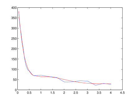
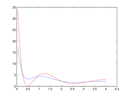
Figure 1: Left: the averages of the aorta intensities (blue) and the estimated Arterial Input Function $\mbox{AIF}(t)$ (red). Right: two curves for distinct spatial locations.

    

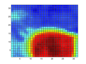
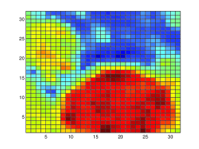
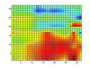
Figure 2: The values of $\widehat{f}$ at 34 seconds (corresponds to the first time point), 95 seconds (the 12th time point) and 275 seconds (the last time point).

7 Proofs.

7.1 Proof of the lower bounds for the risk.

In order to prove Theorem 1, we use Lemma A1 of Bunea et al. (2007), which we will reformulate for the squared risk case.

Lemma 3

Let $\Theta$ be a set of functions of cardinality $\mbox{card\,}(\Theta)\geq 2$ such that
(i) $\|f-g\|^{2}\geq 4\delta^{2},\ for\ f,g\in\Theta,\ f\neq g,$
(ii) the Kullback divergences $K(P_{f},P_{g})$ between the measures $P_{f}$ and $P_{g}$ satisfy the inequality $K(P_{f},P_{g})\leq\log(\mbox{card\,}(\Theta))/16,\ for\ f,\ g\in\Theta$.
Then, for some absolute positive constant $C_{1}$, one has

$$\inf_{f_{n}}\sup_{f\in\Theta}{\mathbb{E}}_{f}\|f_{n}-f\|^{2}\geq C_{1}\delta^{2},$$

where $\inf_{f_{n}}$ denotes the infimum over all estimators.

In order to obtain lower bounds, we introduce a triangular Toeplitz matrix associated with Laurent series $(1-z)^{-r}$ (see Section 8 for more detailed explanations) and denote by $Q^{(L)}=T_{L}\left((1-z)^{-r}\right)$ its reduction to the set of indices $0\leq l\leq L-1$. Following Vareschi (2013), consider function

$$h(t)=\sum_{l=0}^{\infty}h_{l}\varphi_{l}(t)\quad\mbox{with}\ h_{l}=\frac{(-1)^{l}}{\log(l\vee e)}\,{-1/2\choose l}=\frac{\Gamma\left(\frac{1}{2}\right)\,\Gamma\left(\frac{1}{2}+l\right)}{\Gamma(l+1)\,\log(l\vee e)}.$$ (7.1)

Denote $\mbox{$\theta$}^{(L)}=(\theta_{0},\cdots,\theta_{L-1})^{T}=Q^{(L)}\mathbf{h}^{(L)}$ where $\mathbf{h}_{L}$ is the vector of the first $L$ coefficients of function $h$ in (7.1). In what follows we shall use Lemma 6.5 of Vareschi (2013) that was in the original version of the paper posted on ArXiv but did not make it to the published version of Vareschi (2015).

Lemma 4

Let $h(t)$ be as defined in (7.1) and $\mbox{$\theta$}^{(L)}=Q^{(L)}\mathbf{h}^{(L)}$ where $Q^{(L)}=T_{L}\left((1-z)^{-r}\right)$ and $\mathbf{h}^{(L)}$ are reductions of the infinite-dimensional Toeplitz matrix $T\left((1-z)^{-r}\right)$ and vector $\mathbf{h}$ of coefficients of $h(t)$ to the set of indices $0\leq l\leq L-1$. Then, $h(t)$ is square integrable and there exist positive constants $C_{r1}$and $C_{r2}$ that depend on $r$ only such that for all $r\geq 1$ and any $l\geq 0$ one has

$$C_{r1}\,\frac{(l\vee 1)^{r-1/2}}{\log(l\vee e)}\leq\theta_{l}\leq C_{r2}\,(l\vee 1)^{r-1/2}.$$ (7.2)

Let $\vartheta$ be a matrix with components $\vartheta_{k_{1},k_{2}}=\left\{-1,1\right\}$, $k_{1}=0,1,\cdots,2^{j_{1}}-1$, $k_{2}=0,1,\cdots,2^{j_{2}}-1$. Denote the set of all possible values of $\vartheta$ by $\Theta$ and let functions $f_{L,j_{1},j_{2}}$ be of the form

$$f_{L,j_{1},j_{2}}(t,x_{1},x_{2})=\rho\ q_{L}(t)\ p_{j_{1},j_{2}}(x_{1},x_{2}),$$ (7.3)

$$q_{L}(t)=\sum^{L-1}_{l=0}\theta_{l}\,\varphi_{l}(t),\ \ p_{j_{1},j_{2}}(x_{1},x_{2})=\sum^{2^{j_{1}}-1}_{k_{1}=0}\ \sum^{2^{j_{2}}-1}_{k_{2}=0}\vartheta_{k_{1},k_{2}}\,\,\psi_{j_{1},k_{1}}(x_{1})\,\psi_{j_{2},k_{2}}(x_{2}),$$ (7.4)

where $\mbox{$\theta$}^{(L)}$ is the vector with components $\theta_{l}$, $l=0,\cdots,L-1$ where $\mbox{$\theta$}^{(L)}=Q^{(L)}\mathbf{h}^{(L)}$ and $Q^{(L)}$ and $\mathbf{h}^{(L)}$ are defined above. Since $f_{L,j_{1},j_{2}}\in{\cal B}_{\gamma,\beta}^{s_{1},s_{2},s_{3}}(A)$, Lemma 4 implies that one can choose

$$\rho^{2}=C_{r}A^{2}2^{-2j_{1}(s_{1}+\frac{1}{2})-2j_{2}(s_{2}+\frac{1}{2})}\,(L\vee 1)^{-2(r+s_{3})}\,\exp\left\{-2\gamma L^{\beta}\right\},$$ (7.5)

where $0<C_{r}\leq C_{r2}^{2}/2r$. If $\tilde{f}_{L,j_{1},j_{2}}$ is of the form (7.3) but with $\tilde{\vartheta}_{k_{1},k_{2}}\in\Theta$ instead of $\vartheta_{k_{1},k_{2}}$, then, by Lemma 4, the $L^{2}$-norm of the difference is of the form

$$\|\tilde{f}_{L,j_{1},j_{2}}-f_{L,j_{1},j_{2}}\|_{2}^{2}=\rho^{2}\left(\sum^{L-1}_{l=0}\,\theta_{l}^{2}\right)\ \left(\sum^{2^{j_{1}}-1}_{k_{1}=0}\,\sum^{2^{j_{2}}-1}_{k_{2}=0}\,{\mathbb{I}}\left(\tilde{\vartheta}_{k_{1},k_{2}}\neq{\vartheta}_{k_{1},k_{2}}\right)\right)\geq\frac{C_{r1}^{2}\rho^{2}H\left(\tilde{\vartheta},\vartheta\right)(L\vee 1)^{2r}}{2r\,[\log(L\vee e)]^{2}}.$$

Here $H\left(\tilde{\vartheta},\vartheta\right)$ is the Hamming distance between the binary sequences $\mbox{vec}(\vartheta)$ and $\mbox{vec}(\tilde{\vartheta})$ where $\mbox{vec}(\vartheta)$ is a vectorized version of matrix $\vartheta$.

Observe that matrix $\vartheta$ has $\aleph=2^{j_{1}+j_{2}}$ components, and hence, $\mbox{card\,}(\Theta)=2^{\aleph}$. In order to find a lower bound for $H\left(\tilde{\vartheta},\vartheta\right)$, we apply the Varshamov-Gilbert lemma which states that one can choose a subset ${\Theta_{1}}$ of ${\Theta}$, of cardinality of at least $2^{\aleph/8}$, and such that $H\left(\tilde{\vartheta},\vartheta\right)\geq\frac{\aleph}{8}$ for any $\vartheta,\tilde{\vartheta}\in\Theta_{1}$. Hence, for any $\vartheta,\tilde{\vartheta}\in\Theta_{1}$, one has the following expression for $\delta^{2}$ defined in Lemma 3:

$$\|\tilde{f}_{L,j_{1},j_{2}}-f_{L,j_{1},j_{2}}\|^{2}\geq\frac{C_{r1}^{2}\rho^{2}2^{j_{1}+j_{2}}(L\vee 1)^{2r}}{16r\,[\log(L\vee e)]^{2}}=4\delta^{2}.$$ (7.6)

Let $P_{f}$ be the distribution of the process $\left\{f*g(t,{\bf x})+\varepsilon dW(t,{\bf x}),(t,{\bf x})\in U\right\}$ when $f$ is true, where $W(t,{\bf x})$ is a Wiener process. Then, since $\left|\tilde{\vartheta}_{l,k,k^{\prime}}-\vartheta_{l,k,k^{\prime}}\right|\leq 2$, and due to the multiparameter Girsanov formula (see, e.g., Dozzi (1989), p. 89), (7.3) and (7.4), the Kullback divergence can be bounded as

$$K(P_{f},P_{\tilde{f}}) = {\mathbb{E}}_{P_{f}}\left[\log\left(P_{f}/P_{\tilde{f}}\right)\right]=-{\mathbb{E}}_{P_{f}}\left[\varepsilon^{-1}\int_{U}((f-\tilde{f})*g)(t,{\bf x})dW(t,{\bf x})\right]$$ (7.7)

$$+ \left(2\varepsilon^{2}\right)^{-1}\int_{U}\left((f-\tilde{f})*g\right)^{2}(t,{\bf x})dtd{\bf x}$$

$$= \left(2\varepsilon^{2}\right)^{-1}\|(\tilde{f}-f)*g\|_{2}^{2}$$

$$\leq 2\varepsilon^{-2}\,\rho^{2}2^{j_{1}+j_{2}}\|q_{L}*g\|_{2}^{2}=2\varepsilon^{-2}\,\rho^{2}2^{j_{1}+j_{2}}\|G^{(L)}\mbox{$\theta$}^{(L)}\|^{2}_{2},$$

where matrix $G^{(L)}$ and vector $\mbox{$\theta$}^{(L)}$ are defined in (2.7) and Lemma 4, respectively. By Lemma 5 in section 8, and under Assumptions A1 and A2, one obtains that $G^{(L)}=T_{L}((1-z)^{r}v(z))$ and $\|T_{L}(v(z))\|^{2}=\lambda_{\max}[T_{L}^{T}(v(z))T_{L}(v(z))]<\|v\|_{circ}^{2}<\infty$. Therefore, $G^{(L)}\mbox{$\theta$}^{(L)}=G^{(L)}Q^{(L)}\mathbf{h}^{(L)}=T_{L}((1-z)^{r}v(z))T_{L}((1-z)^{-r})\mathbf{h}^{(L)}$ and

$$\|G^{(L)}\mbox{$\theta$}^{(L)}\|_{2}^{2}=\|T_{L}(v(z))\mathbf{h}^{(L)}\|_{2}^{2}\leq\|T_{L}(v(z))\|^{2}\|\mathbf{h}^{(L)}\|_{2}^{2}\leq\|v\|_{circ}^{2}\,\|h\|_{2}^{2}<\infty,$$ (7.8)

where $\|h\|_{2}^{2}$ is the $L^{2}$-norm of the function $h(t)$ and $\|h\|_{2}<\infty$ due to Lemma 4. Combination of (7.7) and (7.8) yields $K(P_{f},P_{\tilde{f}})\leq\tilde{C}\varepsilon^{-2}\rho^{2}2^{j_{1}+j_{2}}/16$ where $\tilde{C}=32\|v\|_{circ}^{2}\|h\|_{2}^{2}$. Application of Lemma 3 requires the constraint

$$K(P_{f},P_{\tilde{f}})\leq\log(\mbox{card\,}(\Theta))/16=\log(2)2^{j_{1}+j_{2}}/16.$$

Therefore, one can choose $\rho^{2}=\varepsilon^{2}/\tilde{C}$, so that, by Lemma 3 for some $C_{1}>0$ one has

$$\inf_{f_{n}}\sup_{f\in\Theta}{\mathbb{E}}_{f}\|f_{n}-f\|^{2}\geq C_{1}\varepsilon^{2}2^{j_{1}+j_{2}}\,(L\vee 1)^{2r}\,[\log(L\vee e)]^{-2},$$ (7.9)

where $L$, $j_{1}$ and $j_{2}$ are such that

$$2^{2j_{1}(s_{1}+\frac{1}{2})+2j_{2}(s_{2}+\frac{1}{2})}\,(L\vee 1)^{2(r+s_{3})}\,\exp\left\{2\gamma L^{\beta}\right\}=C_{2}A^{2}\varepsilon^{-2},$$ (7.10)

with $C_{2}=C_{r}\tilde{C}/\log(2)$. Thus, one needs to choose $j_{1}$, $j_{2}$ and $L$ that maximize $2^{j_{1}+j_{2}}\,(L\vee 1)^{2r}\,[\log(L\vee e)]^{-2}$ subject to condition (7.10). Denote

$$\tau_{\varepsilon}=\log({A^{2}}{\varepsilon^{-2}}).$$ (7.11)

It is easy to check that the solution of the above linear constraint optimization problem is of the form $\left\{j_{1},j_{2},L\right\}=\left\{0,0,\left[A^{2}\varepsilon^{-2}\right]^{\frac{1}{2s_{3}+2r}}\right\}$ if $s_{3}\leq\min\{2rs_{1},2rs_{2}\}$ and $\gamma=\beta=0$, $\left\{j_{1},j_{2},L\right\}=\left\{0,\left(\log(2)\right)^{-1}\left(2s_{2}+1\right)^{-1}\tau_{\varepsilon},e\right\}$ if $s_{1}\geq s_{2}$, $s_{3}\geq 2rs_{2}-2s_{2}-1$ and $\gamma=\beta=0$, $\left\{j_{1},j_{2},L\right\}=\left\{\left(\log(2)\right)^{-1}\left(2s_{1}+1\right)^{-1}\tau_{\varepsilon},0,e\right\}$ if $s_{1}\leq s_{2}$ and $s_{3}\geq 2rs_{1}-2s_{1}-1$ and $\gamma=\beta=0$. $\left\{j_{1},j_{2},L\right\}=\left\{0,\left(\log(2)\right)^{-1}\left(2s_{2}+1\right)^{-1}\tau_{\varepsilon},e\right\}$ if $s_{1}\geq s_{2}$ and $\gamma>0,\beta>0$, and $\left\{j_{1},j_{2},L\right\}=\left\{\left(\log(2)\right)^{-1}\left(2s_{1}+1\right)^{-1}\tau_{\varepsilon},0,e\right\}$ if $s_{1}\leq s_{2}$ and $\gamma>0,\beta>0$. By noting that

$$\frac{s_{3}}{s_{3}+r}\leq\min\left\{\frac{2s_{2}}{2s_{2}+1},\frac{2s_{1}}{2s_{1}+1}\right\},\ \ if\ s_{3}\leq\min\{2rs_{1},2rs_{2}\},\ \ \ \gamma=\beta=0,\\$$ (7.12)

$$\frac{2s_{1}}{2s_{1}+1}\leq\min\left\{\frac{2s_{2}}{2s_{2}+1},\frac{s_{3}}{s_{3}+r}\right\},\ \ if\ s_{1}\leq\min\{{s_{3}}/{2r},s_{2}\},\ \ \ \gamma=\beta=0,\\$$ (7.13)

$$\frac{2s_{2}}{2s_{2}+1}\leq\min\left\{\frac{2s_{1}}{2s_{1}+1},\frac{s_{3}}{s_{3}+r}\right\},\ \ if\ s_{2}\leq\min\{{s_{3}}/{2r},s_{1}\},\ \ \ \gamma=\beta=0,\\$$ (7.14)

and

$$\frac{2s_{1}}{2s_{1}+1}\leq\frac{2s_{2}}{2s_{2}+1},\ \ if\ s_{1}\leq s_{2},\ \ \ \gamma>0,\beta>0,$$ (7.15)

we then choose the highest lower bounds in (7.9). This completes the proof of the theorem.

7.2 Proof of the upper bounds for the risk.

The proof of Lemma 2. Denote the quantities $\widehat{\theta}_{l,\mbox{$\omega$}}-\theta_{l,\mbox{$\omega$}}$ by $\aleph_{l,\mbox{$\omega$}}$, and notice that $\aleph_{l,\mbox{$\omega$}}=\widehat{\theta}_{l,\mbox{$\omega$}}-\theta_{l,\mbox{$\omega$}}=\varepsilon{\bf e_{l}}^{T}\left({\bf G}^{(l)}\right)^{-1}\xi^{(l)}$, where $\xi^{(l)}$ is the $l$-dimensional Gaussian vector such that $\xi^{(l)}\sim N(0,I_{l})$, and ${\bf e_{l}}$ is the $l^{th}$ standard basis vector of dimension $l$. Also, note that $\varepsilon{\bf e}_{l}^{T}({\bf G}^{(l)})^{-1}\xi^{(l)}=\varepsilon\sum^{l-1}_{k=0}v_{k}\xi_{k}$, where $v_{k}$ is defined in Lemma 1. Then, by (4.2), the variance of $\aleph_{l,\mbox{$\omega$}}$ is

$${\mathbb{E}}\left[\aleph_{l,\mbox{$\omega$}}\right]^{2}=\varepsilon^{2}\sum^{l-1}_{k=0}v_{k}^{2}\leq C_{v_{2}}\varepsilon^{2}l^{2r-1}.$$ (7.16)

Now, for the fourth moment of $\aleph_{l,\mbox{$\omega$}}$, and using properties of Gaussian random variables, one has

$${\mathbb{E}}\left[\aleph_{l,\mbox{$\omega$}}\right]^{4} = \varepsilon^{4}{\mathbb{E}}\left[\sum^{l-1}_{k=0}v_{k}\xi_{k}\right]^{4}$$

$$= \varepsilon^{4}\left[\sum^{l-1}_{k=0}v_{k}^{4}{\mathbb{E}}(\xi_{k}^{4})+3\sum^{l-1}_{k_{1},k_{2}=0,k_{1}\neq k_{2}}v^{2}_{k_{1}}v^{2}_{k_{2}}\right]$$

$$= 3\varepsilon^{4}\left[\sum^{l-1}_{k=0}v^{2}_{k}\right]^{2}\leq 3\varepsilon^{4}\left[C_{v_{2}}l^{2r-1}\right]^{2}.$$

This completes the proof of $(\ref{mom4})$. In order to prove formula $(\ref{Largdev})$, recall that $\aleph_{l,\mbox{$\omega$}}\sim N(0,\varepsilon^{2}\sum^{l-1}_{k=0}v_{k}^{2})$. Therefore, by the Gaussian tail probability inequality, one obtains

$$\Pr\left(|\aleph_{l,\mbox{$\omega$}}|>\sqrt{2\tau\ln(\varepsilon^{-1})}\varepsilon\sqrt{\sum^{l-1}_{k=0}v_{k}^{2}}\right)\leq\left[\tau\pi\ln(\varepsilon^{-1})\right]^{-1/2}\varepsilon^{\tau}.$$ (7.17)

Now, since

$$\sum^{l-1}_{k=0}v_{k}^{2}\leq C_{v_{2}}l^{2r-1}\leq\frac{C_{v_{2}}}{C_{G_{1}}}l^{-1}C_{G_{1}}l^{2r}\leq\frac{C_{v_{2}}}{C_{G_{1}}}l^{-1}\|({\bf G}^{(l)})^{-1}\|,$$ (7.18)

$(4.5)$ follows, provided $\nu\geq\tau\frac{C_{v_{2}}}{C_{G_{1}}}$.
The proof of Theorem 2. Denote

$$\mu=\left\{\begin{array}[]{ll}\min\left\{\frac{s_{3}}{s_{3}+r},\frac{2s_{2}}{2s_{2}+1},\frac{2s_{1}}{2s_{1}+1}\right\},\ \ if\ \ \ \gamma=\beta=0,\\ \min\left\{\frac{2s_{2}}{2s_{2}+1},\frac{2s_{1}}{2s_{1}+1}\right\},\ \ \ \ if\ \ \ \ \ \ \gamma>0,\beta>0.\\ \end{array}\right.$$ (7.21)

$$\chi_{\varepsilon,A}=\left[{A^{-2}}{\varepsilon^{2}}\log(1/\varepsilon)\right],$$ (7.22)

$$2^{j_{10}}=\left[\chi_{\varepsilon,A}\right]^{-\frac{\mu}{2s_{1}}},\ \ \ 2^{j_{20}}=\left[\chi_{\varepsilon,A}\right]^{-\frac{\mu}{2s_{2}}},$$ (7.23)

and

$$M_{0}=\left\{\begin{array}[]{ll}\left[\chi_{\varepsilon,A}\right]^{-\frac{\mu}{2s_{3}}}&\mbox{if}\ \ \gamma=\beta=0\\ \left[\frac{\log(1/\varepsilon)}{\gamma}\right]^{1/\beta}&\mbox{if}\ \ \gamma>0,\beta>0,\\ \end{array}\right.$$ (7.26)

and notice that with the choices of $J_{1}$, $J_{2}$ and $M$ given by (4.6), the estimation error can be decomposed into the sum of three components as follows

$${\mathbb{E}}\|\widehat{f}_{n}-f\|^{2}\leq\sum_{\omega}\sum^{\infty}_{l=0}{\mathbb{E}}\|\widehat{\theta}_{l:\mbox{$\omega$}}{\mathbb{I}}\left(|\widehat{\theta}_{l:\mbox{$\omega$}}|>\lambda_{l,\varepsilon}\right)-\theta_{l:\mbox{$\omega$}}\|^{2}\leq R_{1}+R_{2}+R_{3},$$ (7.27)

where

$$R_{1} = \sum^{J_{1}-1}_{j_{1}=0}\sum^{J_{2}-1}_{j_{2}=0}\sum^{M-1}_{l=0}\sum_{k,k^{\prime}}{\mathbb{E}}\left[\left|\widehat{\theta}_{l:\mbox{$\omega$}}-\theta_{l:\mbox{$\omega$}}\right|^{2}{\mathbb{I}}\left(\left|\widehat{\theta}_{l:\mbox{$\omega$}}\right|>\lambda_{l,\varepsilon}\right)\right],$$

$$R_{2} = \sum^{J_{1}-1}_{j_{1}=0}\sum^{J_{2}-1}_{j_{2}=0}\sum^{M-1}_{l=0}\sum_{k,k^{\prime}}\left|{\theta}_{l:\mbox{$\omega$}}\right|^{2}\Pr\left(\left|\widehat{\theta}_{l:\mbox{$\omega$}}\right|<\lambda_{l,\varepsilon}\right),$$

$$R_{3} = \left(\sum^{\infty}_{j_{1}=J_{1}}\sum^{\infty}_{j_{2}=J_{2}}\sum^{\infty}_{l=M}+\sum^{J_{1}-1}_{j_{1}=0}\sum^{\infty}_{j_{2}=J_{2}}\sum^{\infty}_{l=M}+\sum^{\infty}_{j_{1}=J_{1}}\sum^{J_{2}-1}_{j_{2}=0}\sum^{\infty}_{l=M}+\sum^{\infty}_{j_{1}=J_{1}}\sum^{\infty}_{j_{2}=J_{2}}\sum^{M-1}_{l=0}\cdots\right)\sum_{k,k^{\prime}}\left|\theta_{l:\mbox{$\omega$}}\right|^{2}.$$

For $R_{3}$, one uses assumption (3.2) to obtain,

$$R_{3} = O\left(\left(\sum^{J_{1}-1}_{j_{1}=0}\sum^{J_{2}-1}_{j_{2}=0}\sum^{\infty}_{l=M}+\sum^{J_{1}-1}_{j_{1}=0}\sum^{\infty}_{j_{2}=J_{2}}\sum^{M}_{l=1}+\sum^{\infty}_{j_{1}=J_{1}}\sum^{J_{2}-1}_{j_{2}=0}\sum^{M}_{l=1}\right)A^{2}2^{-2j_{1}s_{1}-2j_{2}s_{2}}l^{-2s_{3}}\exp\{-2\gamma l^{\beta}\}\right)$$

$$= O\left(A^{2}2^{-2J_{1}s_{1}}+A^{2}2^{-2J_{2}s_{2}}+A^{2}M^{-2s_{3}}\exp\{-2\gamma M^{\beta}\}\right).$$

If $\gamma=\beta=0$, then since $M\asymp\left[\varepsilon^{2}\right]^{-1/2r}$, $R_{3}$ becomes

$$R_{3} = O\left(A^{2}\left[A^{-2}\varepsilon^{2}\right]^{2s_{1}}+A^{2}\left[A^{-2}\varepsilon^{2}\right]^{2s_{2}}+A^{2}\left[A^{-2}\varepsilon^{2}\right]^{\frac{2s_{3}}{2r}}\right)$$ (7.29)

$$= O\left(A^{2}\left[\chi_{\varepsilon,A}\right]^{\mu}\right).$$

If $\gamma>0,\beta>0$, then

$$R_{3} = O\left(A^{2}\left[A^{-2}\varepsilon^{2}\right]^{2s_{1}}+A^{2}\left[A^{-2}\varepsilon^{2}\right]^{2s_{2}}\right)$$ (7.30)

$$= O\left(A^{2}\left[\chi_{\varepsilon,A}\right]^{\min\left\{\frac{2s_{2}}{2s_{2}+1},\frac{2s_{1}}{2s_{1}+1}\right\}}\right).$$

To evaluate the remaining two terms, notice that both $R_{1}$ and $R_{2}$ can be partitioned into the sum of two error terms as follows

$$R_{1}\leq R_{11}+R_{12},\ \ \ \ R_{2}\leq R_{21}+R_{22},$$ (7.31)

where

$$R_{11} = \sum^{J_{1}-1}_{j_{1}=0}\sum^{J_{2}-1}_{j_{2}=0}\sum^{M}_{l=1}\sum_{k,k^{\prime}}{\mathbb{E}}\left[\left|\widehat{\theta}_{l:\mbox{$\omega$}}-\theta_{l:\mbox{$\omega$}}\right|^{2}{\mathbb{I}}\left(\left|\widehat{\theta}_{l:\mbox{$\omega$}}-\theta_{l:\mbox{$\omega$}}\right|>\frac{1}{2}\lambda_{l;\varepsilon}\right)\right],$$ (7.32)

$$R_{12} = \sum^{J_{1}-1}_{j_{1}=0}\sum^{J_{2}-1}_{j_{2}=0}\sum^{M}_{l=1}\sum_{k,k^{\prime}}{\mathbb{E}}\left[\left|\widehat{\theta}_{l:\mbox{$\omega$}}-\theta_{l:\mbox{$\omega$}}\right|^{2}{\mathbb{I}}\left(\left|\theta_{l:\mbox{$\omega$}}\right|>\frac{1}{2}\lambda_{l;\varepsilon}\right)\right],$$ (7.33)

$$R_{21} = \sum^{J_{1}-1}_{j_{1}=0}\sum^{J_{2}-1}_{j_{2}=0}\sum^{M}_{l=1}\sum_{k,k^{\prime}}\left|\theta_{l:\mbox{$\omega$}}\right|^{2}\Pr\left(\left|\widehat{\theta}_{l:\mbox{$\omega$}}-\theta_{l:\mbox{$\omega$}}\right|>\frac{1}{2}\lambda_{l;\varepsilon}\right),$$ (7.34)

$$R_{22} = \sum^{J_{1}-1}_{j_{1}=0}\sum^{J_{2}-1}_{j_{2}=0}\sum^{M}_{l=1}\sum_{k,k^{\prime}}\left|\theta_{l:\mbox{$\omega$}}\right|^{2}{\mathbb{I}}\left(\left|\theta_{l:\mbox{$\omega$}}\right|<\frac{3}{2}\lambda_{l;\varepsilon}\right).$$ (7.35)

Combining (7.32) and (7.34) and applying Cauchy-Schwarz inequality, Lemma 2 and the fact that $M\asymp\left[\varepsilon^{2}\right]^{-1/2r}$, yields

$$R_{11}+R_{21} = O\left(\sum^{J_{1}-1}_{j_{1}=0}\sum^{J_{2}-1}_{j_{2}=0}\sum^{M}_{l=1}\left(2^{j_{1}+j_{2}}\varepsilon^{2}l^{2r-1}\varepsilon^{\tau/2}+\varepsilon^{\tau}\sum_{k,k^{\prime}}\left|\theta_{l:\mbox{$\omega$}}\right|^{2}\right)\right)$$

$$= O\left({\varepsilon^{2}}2^{J_{1}+J_{2}}M^{2r}\left({\varepsilon^{2}}\right)^{\frac{\tau}{4}}+A^{2}\varepsilon^{\tau}\right)$$

$$= O\left(A^{4}\left({\varepsilon^{2}}\right)^{\frac{\tau}{4}-2}+A^{2}\varepsilon^{\tau}\right).$$

Hence, for $\tau\geq 12$ and under condition (4.8), as $\varepsilon\rightarrow 0$, one has

$$R_{11}+R_{21}=O\left(\varepsilon^{2}\right)=O\left(A^{2}\left[\chi_{\varepsilon,A}\right]^{\mu}\right).$$ (7.36)

Now, combining (7.33) and (7.35), and using (4.3) and (4.7), one obtains

$$\Delta=R_{12}+R_{22} = O\left(\sum^{J_{1}-1}_{j_{1}=0}\sum^{J_{2}-1}_{j_{2}=0}\sum^{M}_{l=1}\sum_{k,k^{\prime}}\min\left\{\left|\theta_{l:\mbox{$\omega$}}\right|^{2},{\varepsilon^{2}}\log(1/\varepsilon)l^{-1}\|(\mathbf{G}^{(l)})^{-1}\|^{2}\right\}\right)$$ (7.37)

$$= O\left(\sum^{J_{1}-1}_{j_{1}=0}\sum^{J_{2}-1}_{j_{2}=0}\sum^{M}_{l=1}\min\left\{\sum_{k,k^{\prime}}\left|\theta_{l:\mbox{$\omega$}}\right|^{2},2^{j_{1}+j_{2}}{\varepsilon^{2}}\log(1/\varepsilon)l^{2r-1}\right\}\right).$$

Then, $\Delta$ can be decomposed into three components, $\Delta_{1}$, $\Delta_{2}$ and $\Delta_{3}$, as follows

$$\Delta_{1} = O\left(\left(\sum^{J_{1}-1}_{j_{1}=j_{10}+1}\sum^{J_{2}-1}_{j_{2}=0}\sum^{M}_{l=1}+\sum^{J_{1}-1}_{j_{1}=0}\sum^{J_{2}-1}_{j_{2}=j_{20}+1}\sum^{M}_{l=1}+\sum^{J_{1}-1}_{j_{1}=0}\sum^{J_{2}-1}_{j_{2}=0}\sum^{M}_{l=M_{0}}\right)\sum_{k,k^{\prime}}\left|\theta_{l:\mbox{$\omega$}}\right|^{2}\right),$$ (7.38)

$$\Delta_{2} = O\left(\sum^{j_{10}}_{j_{1}=0}\sum^{j_{20}}_{j_{2}=0}\sum^{M_{0}}_{l=1}A^{2}2^{j_{1}+j_{2}}\left[\chi_{\varepsilon,A}\right]l^{2r-1}{\mathbb{I}}\left(\eta^{c}_{l:j_{1},j_{2}}\right)\right),$$ (7.39)

$$\Delta_{3} = O\left(\sum^{j_{10}}_{j_{1}=0}\sum^{j_{20}}_{j_{2}=0}\sum^{M_{0}}_{l=1}\left[\sum_{k,k^{\prime}}\left|\theta_{l:\mbox{$\omega$}}\right|^{2}\right]{\mathbb{I}}\left(\eta_{l:j_{1},j_{2}}\right)\right),$$ (7.40)

where $\eta_{l:j_{1},j_{2}}=\left\{l,j_{1},j_{2}:2^{j_{1}+j_{2}}l^{2r}>\left[\chi_{\varepsilon,A}\right]^{\mu-1}\right\}$. For $\Delta_{1}$, it is easy to see that for $j_{10}$, $j_{20}$ and $M_{0}$ given in (7.23) and (7.26), respectively,

$$\Delta_{1} = O\left(A^{2}2^{-2j_{10}s_{1}}+A^{2}2^{-2j_{20}s_{2}}+A^{2}M_{0}^{-2s_{3}}\exp\{-2\gamma M_{0}^{\beta}\}\right).$$

Consequently, if $\gamma=\beta=0$, as $\varepsilon\rightarrow 0$, one has

$$\Delta_{1}=O\left(A^{2}\left[\chi_{\varepsilon,A}\right]^{\mu}\right).$$ (7.41)

If $\gamma>0,\beta>0$, then

$$\Delta_{1} = O\left(A^{2}2^{-2j_{10}s_{1}}+A^{2}2^{-2j_{20}s_{2}}\right)$$ (7.42)

$$= O\left(A^{2}\left[\chi_{\varepsilon,A}\right]^{\min\left\{\frac{2s_{2}}{2s_{2}+1},\frac{2s_{1}}{2s_{1}+1}\right\}}\right).$$

For $\Delta_{2}$ in (7.39), as $\varepsilon\rightarrow 0$, one obtains

$$\Delta_{2}=O\left(A^{2}\left[A^{-2}{\varepsilon^{2}}\log(1/\varepsilon)\right]\left[\chi_{\varepsilon,A}\right]^{\mu-1}\right)=O\left(A^{2}\left[\chi^{\alpha}_{\varepsilon,A}\right]^{\mu}\right).$$ (7.43)

In order to evaluate (7.40), we need to consider five different cases.
Case 1: $\gamma=\beta=0$, $s_{1}\leq\min\{s_{2},\frac{s_{3}}{2r}\}$. In this case, $\mu=\frac{2s_{1}}{2s_{1}+1}$, (7.40) becomes, as $\varepsilon\rightarrow 0$

$$\Delta_{3} = O\left(A^{2}\sum^{j_{10}}_{j_{1}=0}\sum^{M_{0}}_{l=1}\sum^{j_{20}}_{j_{2}=0}2^{-2j_{1}s_{1}-2j_{2}s_{2}}l^{-2s_{3}}{\mathbb{I}}\left(2^{j_{1}}>2^{-j_{2}}\frac{\left[\chi_{\varepsilon,A}\right]^{\mu-1}}{l^{2r}}\right)\right)$$ (7.44)

$$= O\left(A^{2}\left[\chi_{\varepsilon,A}\right]^{2s_{1}(1-\mu)}\sum^{M_{0}}_{l=1}l^{-2(s_{3}-s_{1}2r)}\sum^{j_{20}}_{j_{2}=0}2^{-2j_{2}(s_{2}-s_{1})}\right)$$

$$= O\left(A^{2}\left[\chi_{\varepsilon,A}\right]^{\frac{2s_{1}}{2s_{1}+1}}\left[\log(\varepsilon^{-1})\right]^{{\mathbb{I}}(s_{1}=s_{2})+{\mathbb{I}}(s_{1}=s_{3}/2r)}\right).$$

Case 2: $\gamma=\beta=0$, $s_{2}\leq\min\{s_{1},\frac{s_{3}}{2r}\}$. In this case, $\mu=\frac{2s_{2}}{2s_{2}+1}$, (7.40) becomes, as $\varepsilon\rightarrow 0$

$$\Delta_{3} = O\left(A^{2}\sum^{j_{10}}_{j_{1}=0}\sum^{M_{0}}_{l=1}\sum^{j_{20}}_{j_{2}=0}2^{-2j_{1}s_{1}-2j_{2}s_{2}}l^{-2s_{3}}{\mathbb{I}}\left(2^{j_{2}}>2^{-j_{1}}\frac{\left[\chi_{\varepsilon,A}\right]^{\mu-1}}{l^{2r}}\right)\right)$$ (7.45)

$$= O\left(A^{2}\left[\chi_{\varepsilon,A}\right]^{2s_{2}(1-\mu)}\sum^{M_{0}}_{l=1}l^{-2(s_{3}-s_{2}2r)}\sum^{j_{10}}_{j_{1}=0}2^{-2j_{1}(s_{1}-s_{2})}\right)$$

$$= O\left(A^{2}\left[\chi_{\varepsilon,A}\right]^{\frac{2s_{2}}{2s_{2}+1}}\left[\log(\varepsilon^{-1})\right]^{{\mathbb{I}}(s_{1}=s_{2})+{\mathbb{I}}(s_{2}=s_{3}/2r)}\right).$$

Case 3: $\gamma=\beta=0$, $s_{3}\leq\min\{2rs_{1},{2rs_{2}}\}$. In this case, $\mu=\frac{2s_{3}}{2s_{3}+2r}$, (7.40) becomes, as $\varepsilon\rightarrow 0$

$$\Delta_{3} = O\left(A^{2}\sum^{j_{10}}_{j_{1}=0}\sum^{M_{0}}_{l=1}\sum^{j_{20}}_{j_{2}=0}2^{-2j_{1}s_{1}-2j_{2}s_{2}}l^{-2s_{3}}{\mathbb{I}}\left(l^{2r}>2^{-j_{1}-j_{2}}{\left[\chi_{\varepsilon,A}\right]^{\mu-1}}{}\right)\right)$$ (7.46)

$$= O\left(A^{2}\left[\chi_{\varepsilon,A}\right]^{-\frac{\mu-1}{2r}2s_{3}}\sum^{j_{10}}_{j_{1}=0}2^{-\frac{2j_{1}}{2r}(2rs_{1}-s_{3})}\sum^{j_{20}}_{j_{2}=0}2^{-\frac{2j_{2}}{2r}(2rs_{2}-s_{3})}\right)$$

$$= O\left(A^{2}\left[\chi_{\varepsilon,A}\right]^{\frac{s_{3}}{s_{3}+r}}\left[\log(\varepsilon^{-1})\right]^{{\mathbb{I}}(s_{2}=s_{3}/2r)+{\mathbb{I}}(s_{1}=s_{3}/2r)}\right).$$

Case 4: $\gamma>0,\beta>0$, $s_{1}\leq s_{2}$. In this case, $\mu=\frac{2s_{1}}{2s_{1}+1}$, (7.40) becomes, as $\varepsilon\rightarrow 0$

$$\Delta_{3} = O\left(A^{2}\sum^{j_{10}}_{j_{1}=0}\sum^{M_{0}}_{l=1}\sum^{j_{20}}_{j_{2}=0}2^{-2j_{1}s_{1}-2j_{2}s_{2}}l^{-2s_{3}}\exp\{-2\gamma l^{\beta}\}{\mathbb{I}}\left(2^{j_{1}}>2^{-j_{2}}\frac{\left[\chi_{\varepsilon,A}\right]^{\mu-1}}{l^{2r}}\right)\right)$$ (7.47)

$$= O\left(A^{2}\left[\chi_{\varepsilon,A}\right]^{\frac{2s_{1}}{2s_{1}+1}}\sum^{j_{20}}_{j_{2}=0}2^{-2j_{2}(s_{2}-s_{1})}\right)$$

$$= O\left(A^{2}\left[\chi_{\varepsilon,A}\right]^{\frac{2s_{1}}{2s_{1}+1}}\left[\log(\varepsilon^{-1})\right]^{{\mathbb{I}}(s_{1}=s_{2})}\right).$$

Case 5: $\gamma>0,\beta>0$, $s_{2}\leq s_{1}$. In this case, $\mu=\frac{2s_{2}}{2s_{2}+1}$, (7.40) becomes, as $\varepsilon\rightarrow 0$

$$\Delta_{3} = O\left(A^{2}\sum^{j_{10}}_{j_{1}=0}\sum^{M_{0}}_{l=1}\sum^{j_{20}}_{j_{2}=0}2^{-2j_{1}s_{1}-2j_{2}s_{2}}l^{-2s_{3}}\exp\{-2\gamma l^{\beta}\}{\mathbb{I}}\left(2^{j_{2}}>2^{-j_{1}}\frac{\left[\chi_{\varepsilon,A}\right]^{\mu-1}}{l^{2r}}\right)\right)$$ (7.48)

$$= O\left(A^{2}\left[\chi_{\varepsilon,A}\right]^{\frac{2s_{2}}{2s_{2}+1}}\sum^{j_{10}}_{j_{1}=0}2^{-2j_{1}(s_{1}-s_{2})}\right)$$

$$= O\left(A^{2}\left[\chi_{\varepsilon,A}\right]^{\frac{2s_{2}}{2s_{2}+1}}\left[\log(\varepsilon^{-1})\right]^{{\mathbb{I}}(s_{1}=s_{2})}\right).$$

Now, to complete the proof, combine formulae (7.29)-(7.48).

8 Introduction to the theory of banded Toeplitz matrices.

The proof of asymptotic optimality of the estimator ${\hat{f}}$ relies heavily on the theory of banded Toeplitz matrices developed in Böttcher and Grudsky (2000, 2005). In this subsection, we review some of the facts about Toeplitz matrices which were used in the proofs in Section 7.

Consider a sequence of numbers $\{b_{k}\}_{k=-\infty}^{\infty}$ such that $\sum_{k=-\infty}^{\infty}|b_{k}|<\infty$. An infinite Toeplitz matrix $T=T(b)$ is the matrix with elements $T_{i,j}=b_{i-j}$, $i,j=0,1,\ldots$.

Let ${\cal C}=\{z\in C:|z|=1\}$ be the complex unit circle. With each Toeplitz matrix $T(b)$ we can associate its symbol

$$b(z)=\sum_{k=-\infty}^{\infty}b_{k}z^{k},\ \ z\in{\cal C}.$$ (8.49)

Since, $\displaystyle{B(\theta)=b(e^{i\theta})=\sum_{k=-\infty}^{\infty}b_{k}e^{ik\theta}}$, numbers $b_{k}$ are Fourier coefficients of function $B(\theta)=b(e^{i\theta})$. For any function $b(z)$ with an argument on a unit circle ${\cal C}$ denote

$$\|b\|_{circ}=\displaystyle{\max_{|z|=1}b(z)}.$$

There is a very strong link between properties of a Toeplitz matrix $T(b)$ and function $b(z)$. In particular, if $b(z)\neq 0$ for $z\in{\cal C}$ and $\mbox{wind}(b)=J_{b}$, then $b(z)$ allows Wiener-Hopf factorization $b(z)=b_{-}(z)\,b_{+}(z)\,z^{J_{b}}$ where $b_{+}$ and $b_{-}$ have the following forms

$$b_{-}(z)=\sum_{k=0}^{\infty}b^{-}_{-k}z^{-k},\ \ b_{+}(z)=\sum_{k=0}^{\infty}b^{+}_{k}z^{k}$$

(see Theorem 1.8 of Böttcher and Grudsky (2005)).

If $T(b)$ is a lower triangular Toeplitz matrix, then $b(z)\equiv b_{+}(z)$ with $b^{+}_{k}=b_{k}$. In this case, the product of two Toeplitz matrices can be obtained by simply multiplying their symbols and the inverse of a Toeplitz matrix can be obtained by taking the reciprocal of function $b_{+}(z)$:

$$T(b_{+}d_{+})=T(b_{+})T(d_{+}),\ \ \ T^{-1}(b_{+})=T(1/b_{+}).$$ (8.50)

Let $T_{m}(b)=T_{m}(b_{+})\in R^{m\times m}$ be a banded lower triangular Toeplitz matrix corresponding to the Laurent polynomial $\displaystyle{b(z)=\sum_{k=0}^{m-1}b_{k}z^{k}}$.

In practice, one usually use only finite, banded, Toeplitz matrices with elements $T_{i,j}$, $i,j=0,1,\ldots,m-1$. In this case, only a finite number of coefficients $b_{k}$ do not vanish and function $b(z)$ in (8.49) reduces to a Laurent polynomial $\displaystyle{b(z)=\sum_{k=-J}^{K}b_{k}z^{k}}$, $z\in{\cal C}$, where $J$ and $K$ are nonnegative integers, $b_{-J}\neq 0$ and $b_{K}\neq 0$. If $b(z)\neq 0$ for $z\in{\cal C}$, then $b(z)$ can be represented in a form

$$b(z)=z^{-J}b_{K}\prod_{j=1}^{J_{0}}(z-\mu_{j})\prod_{k=1}^{K_{0}}(z-\nu_{k})\ \ \mbox{with}\ \ |\mu_{j}|<1,\,|\nu_{k}|>1.$$ (8.51)

In this case, the winding number of $b(z)$ is $\mbox{wind}(b)=J_{0}-J$.

Let $T_{m}(b)=T_{m}(b_{+})\in R^{m\times m}$ be a banded lower triangular Toeplitz matrix corresponding to the Laurent polynomial $\displaystyle{b(z)=\sum_{k=0}^{m-1}b_{k}z^{k}}$. If $b$ has no zeros on the complex unit circle ${\cal C}$ and $\mbox{wind}(b)=0$, then, due to Theorem 3.7 of Böttcher and Grudsky (2005), $T(b)$ is invertible and $\displaystyle{\lim_{m\rightarrow\infty}\sup\rho(T_{m}^{-1}(b))<\infty}$. Moreover, by Corollary 3.8,

$$\lim_{m\rightarrow\infty}\rho(T_{m}^{-1}(b))=\rho(T^{-1}(b))$$ (8.52)

In the paper, we need the following result that is a combination of Lemmas 3 and 4 of Comte et al. (2017).

Lemma 5

Let function $g$ in (1.1) satisfy Assumptions A1 and A2. Then, $G^{(L)}=T_{L}((1-z)^{r}v(z))$ where function $v(z)$ has all its zeros outside the complex unit circle, so that $\|T_{L}(v(z))\|^{2}=\lambda_{\max}[T_{L}^{T}(v(z))T_{L}(v(z))]<\|v\|_{circ}^{2}<\infty$.

References

- [1] Abramovich, F., Pensky, M., Rozenholc, Y. (2013). Laplace deconvolution with noisy observations. Electron. J. Stat. 7, 1094-1128.
- [2] Benhaddou, R., Pensky, M., Picard, D. (2013). Anisotropic denoising in functional deconvolution model with dimension-free convergence rates. Electron. J. Stat. 7, 1686-1715.
- [3] Bisdas, S., Konstantinou, G.N., Lee, P.S., Thng, C.H., Wagenblast, J., Baghi, M., Koh, T.S. (2007). Dynamic contrast-enhanced CT of head and neck tumors: perfusion measurements using a distributed-parameter tracer kinetic model. Initial results and comparison with deconvolution- based analysis. Physics in Medicine and Biology. 52, 6181-6196.
- [4] Böttcher, A., and Grudsky, S.M. (2000). Toeplitz Matrices, Asymptotic Linear Algebra, and Functional Analysis. Birkhauser Verlag, Basel-Boston-Berlin.
- [5] Böttcher, A., and Grudsky, S.M. (2005). Spectral Properties of Banded Toeplitz Matrices, SIAM, Philadelphia.
- [6] Brown, L.D. and Low, M.G. (1996). Asymptotic equivalence of nonparametric regression and white noise. Ann. Statist., 24, 2384–2398.
- [7] Bunea, F., Tsybakov, A. and Wegkamp, M.H. (2007). Aggregation for Gaussian regression. Ann. Statist. 35, 1674–1697.
- [8] Cao, Y. (2011). The promise of dynamic contrast-enhanced imaging in radiation therapy. Semin Radiat Oncol. 2, 147–56.
- [9] Cao, M., Liang, Y., Shen, C., Miller, K.D., Stantz, K.M. (2010). Developing DCE-CT to quantify Intra-Tumor heterogeneity in breast tumors with differing angiogenic phenotype. IEEE Trans. on Medical Imaging. 29, 1089–1092.
- [10] Comte, F., Cuenod, C.-A., Pensky, M., Rozenholc, Y. (2017). Laplace deconvolution on the basis of time domain data and its application to Dynamic Contrast Enhanced imaging. Journ. Royal Stat. Soc., Ser.B. 79, 69–94
- [11] Comte, F., Genon-Catalot, V. (2015). Adaptive Laguerre density estimation for a mixed Poisson model. Electron. J. Stat. 9, 1113–1149
- [12] Cuenod, C.F., Favetto, B., Genon-Catalot, V., Rozenholc, Y., Samson, A. (2011). Parameter estimation and change-point detection from Dynamic Contrast Enhanced MRI data using stochastic differential equations. Math. Biosci. 233, 68–76
- [13] Dey, A.K., Martin, C.F., Ruymgaart, F.H. (1998). Input recovery from noisy output data, using regularized inversion of Laplace transform. IEEE Trans. Inform. Theory. 44, 1125–1130.
- [14] Dozzi, M. (1989). Stochastic Processes with a Multidimensional Parameter. Longman Scientific & Technical, New York.
- [15] Gradshtein, I.S., Ryzhik, I.M. (1980). Tables of integrals, series, and products. Academic Press, New York.
- [16] Mabon, G. (2016). Adaptive deconvolution of linear functionals on the nonnegative real line. Journ. Statist. Plan. Inf. 178, 1-23.
- [17] REMISCAN - Project number IDRCB 2007-A00518-45/P060407/STIC 2006; Research Ethics Board (REB) approved- cohort funding by INCa (1M Euros) and promoted by the AP-HP (Assistance Publique Hôpitaux de Paris). Inclusion target: 100 patients. Start in 2007. Closed since July 2015.
- [18] Rozenholc, Y., Reiß, M. (2012) Preserving time structures while denoising a dynamical image, Mathematical Methods for Signal and Image Analysis and Representation (Chapter 12), Florack, L. and Duits, R. and Jongbloed, G. and van Lieshout, M.-C. and Davies, L. Ed., Springer-Verlag, Berlin.
- [19] Vareschi, T. (2013). Noisy Laplace deconvolution with error in the operator. ArXiv 1303.7437, version 2.
- [20] Vareschi, T. (2015). Noisy Laplace deconvolution with error in the operator. Journ. Statist. Plan. Inf. 157-158, 16-35.