Diffusiophoretic Enhancement of Mass Transfer by Nanofluids

Abstract

Observations of an enhanced mass transfer in nanofluids have led to several propositions for the underlying cause, but none of them have been clearly established. Here, we reproduce the enhancement phenomenon within a glass capillary containing fluorescein di-sodium dye solution on one side and alumina nanoparticle suspension on the other, avoiding convective interferences present earlier. The enhancement is explained by the counter-convective motion of the dye solution in response to the diffusiophoretic motion of the nanoparticles towards a higher concentration of the dye. The velocity of the dye front agrees with the theoretical estimate obtained from the diffusiophoretic velocity of alumina nanoparticles in a gradient of fluorescein di-sodium electrolyte solution. With a suitably chosen nanofluid, it should now be possible to effect the enhancement (or suppression) of mass transfer of a given solute.

ToC Graphic

I Introduction

The presence of a small fraction of nanoparticles as a suspension in a fluid (also referred to as nanofluids) seems to immensely influence various phenomenon like diffusion Krishnamurthy et al. (2006); Fang et al. (2009); Veilleux and Coulombe (2010), absorption Komati and Suresh (2010); Pang et al. (2012); Olle et al. (2006); Esmaeili-Faraj and Nasr Esfahany (2016); Moraveji et al. (2013); Rahmatmand et al. (2016), extraction Mirzazadeh Ghanadi et al. (2015); Saien and Bamdadi (2012); Ashrafmansouri et al. (2016), in radiationWaheed et al. (2015), electric conductivity Liu et al. (2016), evaporation Javed et al. (2013) and reaction kinetics of chemical processes. Mass transfer studies in dye-diffusion by Krishnamurthy et al. 2006 and others Veilleux and Coulombe (2010); Fang et al. (2009) have demonstrated, through dramatic visual effects, that the presence of nanoparticles increases the effective diffusivity up to 14 folds. Yet, when carried out in other system configurations, there are some cases where no enhancement Ozturk et al. (2010); Subba-Rao et al. (2011) and even a lowering of the diffusivity Turanov and Tolmachev (2009); Gerardi et al. (2009); Feng and Johnson (2012) are observed. Various possibilities have been advanced in an attempt to explain these intriguing observations: Brownian motion, micro-convection Fang et al. (2009); Krishnamurthy et al. (2006), interfacial complexationOzturk et al. (2010), dispersion model Veilleux and Coulombe (2011), etc., but none of them have been backed with conclusive evidence. Here, we explore our hypothesis that the enhancement is because of a diffusiophoretic motion Prieve et al. (1984) of the nanoparticles, a well established concept in colloidal physics, resulting in a counter convective motion of the dye (or other solute) molecules, leading to an increase in the observed diffusivity of the solute.

We first elaborate the contrasting observations on the effect of nanoparticles. For a homogeneously mixed system, where the nanoparticles and the solute are uniformly dispersed, and the diffusivity is measured using Fluorescence Correlation Spectroscopy (FCS)Subba-Rao et al. (2011) or Nuclear magnetic resonance (NMR)Turanov and Tolmachev (2009); Gerardi et al. (2009), no enhancement or a small lowering of the diffusivity of the solute has been reported. A significant enhancement is observed only in an inhomogeneous system (various configurations are shown in Figure 1) Krishnamurthy et al. (2006); Fang et al. (2009); Veilleux and Coulombe (2010). However, even here there are instances where there is little enhancement Ozturk et al. (2010) or even a decrease in the apparent diffusivity of the soluteFeng and Johnson (2012).

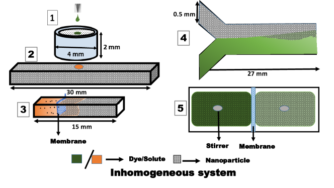
Figure 1: Schematic of a few inhomogeneous systems where the effect of nanoparticles on the diffusivity of a solute were studied. 1: Dye drop set up of Krishnamurthy et al. 2006, and of 2: Fang et al. 2009. 3: Membrane barrier diffusion of Veilleux and Coulombe 2010. 4: Microfluidic setup of Ozturk et al. 2010, 5: Diffusion cell of Feng and Johnson 2012. In the last two cases, no enhancement of the solute diffusivity was observed.

Given the ubiquitous presence of a gradient in the dye or other solute concentrations, we propose that the anomalous increase in diffusivity is due to diffusiophoresis. Diffusiophoresis is the phoretic motion of rigid colloidal particles in the presence of a gradient in the concentration of a solute that interacts with the surface of the colloidal particle. Diffusiophoresis is a well-known phenomenon since the last century, and Derjaguin et al. 1961 provided a simple expression for the particle velocity. The most comprehensive derivation of the equations of motion of the particles for Brownian and non-Brownian suspensions has been recently published Brady (2011) for non-electrolyte suspensions. Depending on the nature of the interaction, attractive or repulsive, the particle experiences a positive or negative velocity, respectively, along the direction of the positive concentration gradient. The micro-mechanical origin of this velocity is due to a solute induced gradient in the normal stresses in the fluid surrounding the particle, that is balanced by the viscous forces at the surface of the solid Anderson et al. (1982); Prieve (2008). Our postulate is that the drift motion of nanoparticles in a concentration gradient induces a counter-convective motion of the solvent containing the dye molecules leading to an increase in their spread, which is often reported as an increase in the diffusivity.

In this work we construct a system identical in the fundamental phenomenology to the system used in the dye-drop experiment Krishnamurthy et al. (2006), but without the bulk convective effects resulting from the inertial motion as the drop is dispensed in the liquid. To achieve this, we recognize that when a drop of dye is placed in a suspension of nanoparticles, an interface between two nearly “stationary” fluids is created—one side being the solution of dye in water and the other side is the suspension of nanoparticles. By using a controlled system having a similar configuration, we avoid the irregular motion observed in the earlier work Krishnamurthy et al. (2006), measure the initial velocity of the dye front and compare it with the estimate obtained using the diffusiophoretic velocity of the nanoparticles.

II Methodology

A non-flow (one end sealed) glass capillary (I.D. 1 mm, length 6 cm) is first filled with a dispersion of nanoparticles (alumina, 13 nm diameter, from Sigma Aldrich) in water, as shown in the schematic in Figure 2. This is followed by injecting a dye solution (fluorescein di-sodium with a molecular weight of 376.27 g/mol, from Himedia Laboratories) leaving an air gap in between. The air bubble is then gently sucked out using a blunt needled (25 gauge) syringe, causing the outer fluid to close upon forming a stationary nearly straight interface (the sealed end prevents a bulk motion of the nanofluid)Dalia (2012). The open end is finally sealed using paraffin wax or film.

The nanoparticle suspension is charge stabilized with ethane-diol (0.5% v/v) and NaOH ( % v/v) at a pH of 9, which shows a greater extent of stabilization with zeta value 39.6$\pm$1.2 mV, than the other surfactant based systems (Zeta of alumina in water is 3.9$\pm$0.4 mV). Earlier studies Krishnamurthy et al. (2006) have mostly used Tween-80, but we find that the stabilization with Tween-80 is not adequate for the horizontal capillary system: the nanoparticles settle down during the period of the experiment, leading to secondary convective flows which can also influence the spread of the dye. Ethane-diol also reduces interfacial complexation with flourescein Ozturk et al. (2010), with the observed visual absence of intensified fluorescent band. An equal percentage of ethane-diol–NaOH is also present in the aqueous (dye) phase, to prevent any concentration gradient induced effects.

This entire capillary set-up is placed inside a temperature regulated dark box with a UV light source. Digital images are captured using Nikon D90 DSLR (50-70mm lens, f/3.3-f/4.5), at programmed regular intervals using a camera control software (DIYPhotobits). The images are processed in Matlab-R2015a image processing toolbox, where the intensity of the green channel is extracted. The concentration of the dye has been chosen to be below 2 mM (the critical concentration above which dimerization of the dye leads to quenching) so that the intensity of the fluorescently emitted light is linearly proportional to the concentration of the dyeArbeloa (1981).

The concentration profile of the dye follows a nearly sigmoid pattern shown in Figure 2, which can be fit to an equation

$$C=a+b\,\mathrm{erf}\left(\frac{x-x_{0}}{m}\right).$$ (1)

Here, $x_{0}$ denotes the center of the interfacial region, and $m$ is a characteristic width of the interface, $a$ and $b$ are other constants. The dye diffusivity ($\mathcal{D}$) can be derived as

$$\mathcal{D}=\frac{1}{4}\,\frac{\mathrm{d}m^{2}}{\mathrm{d}t}\Bigg{\arrowvert}_{t=0}.$$ (2)

In the absence of nanoparticles, the dye front diffuses through the aqueous phase with ethane-diol–NaOH (this is similar to the experiment where a dye drop is added to pure water in the earlier work Krishnamurthy et al. (2006)). The diffusivity calculated by the above method is found to be 600 $\pm$57 $\mu$m²/s. This is within 6-15% of the values reported earlier Culbertson et al. (2002); Saltzman et al. (1994); Casalini et al. (2011), thus validating our method of analyzing the propagation of the dye front. The presence of ethane-diol also has negligible influence on the diffusivity of flourescein.

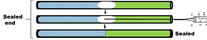
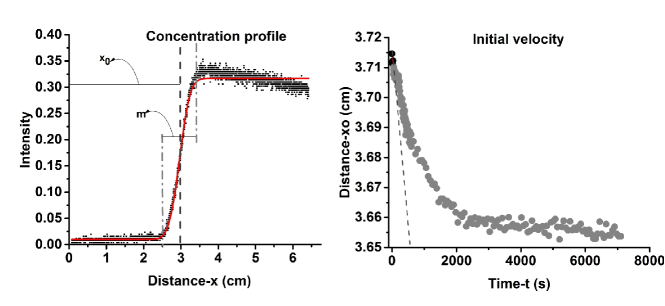
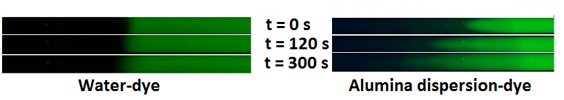
Figure 2: (a) Schematic of steps for forming a stationary interface inside a capillary (b) Extraction of the initial velocity from intensity profiles at various times (c) Images of dye front captured at various time instances (in seconds) placed against water and nanofluid.

III Results and discussion

We now present the main results of the motion of the dye front into a suspension of nanoparticles. When the dye front comes in contact with the nanofluid front, the motion of the dye is relatively dramatic (similar to the what was reported in the dye-drop experiment), as shown in Figure 2 compared to the nearly still front in the absence of alumina particles. The time evolution of the concentration profile is also different, that we find it better described by a linear translation the dye front. The front velocity (${\mathrm{d}x_{0}}/{\mathrm{d}t}$) is maximum at the beginning and slowly tapers off to zero with time, as can be inferred from Figure 2. For the purpose of this study we limit the discussion to the initial velocity of the dye front

$$V_{\mathrm{dye}}=\frac{\mathrm{d}x_{0}}{\mathrm{d}t}\Bigg{\arrowvert}_{t=0}.$$ (3)

The effect of alumina nanoparticle concentration on $V_{\mathrm{dye}}$ for a fixed dye concentration (0.1 mM) is shown in Figure 3. The velocities are comparable to the velocities obtained in the dye-drop experiment Krishnamurthy et al. (2006), implying the phenomenon occurring in the horizontal capillary system is similar to the former. The effect of dye concentration on $V_{\mathrm{dye}}$, shown in Figure 3, has not been reported in the earlier experiments. This is also crucial to infer the nature of the driving.

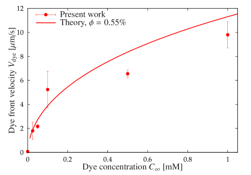
Figure 3: Dependence of the velocity of the dye front (a) Effect of initial nanoparticle concentration (with an initial dye concentration 0.1 mM), compared with the results reported by Krishnamurthy et al. 2006 (with an initial dye concentration of 1 mM) (b) Effect of initial dye concentration at a nanoparticle concentration of 0.55% (v/v). In both the plots the lines are the theoretical velocity evaluated from Equation (13).

Diffusiophoresis can explain the enhanced motion observed in Figure 3. Fluorescein (which is the solute here) is known to interact with alumina nanoparticles forming a surface complex Ozturk et al. (2010) (in essence an attractive interaction). When the nanofluid phase comes in contact with the dye phase, the nanoparticles at the interface are effectively placed in a steep gradient, with the dye only on one side of the nanoparticles at the interface. This causes a motion of the nanoparticles towards the dye phase by diffusiophoresis (towards a higher concentration of the dye due to the attractive interaction). Since the ends of the capillary are sealed, incompressibility of the fluid implies that an equal volume of dye bearing fluid will move towards the nanofluid phase, which is visually observed as an enhanced motion, more than the normal dye diffusion.

This behavior can be quantified more precisely using the diffusiophoretic velocity experienced by a nanoparticle placed in a gradient of an electrolyte. Whereas the expressions derived in the references cited earlier Anderson et al. (1982); Brady (2011) deal with a case when the solute is a non-electrolyte, the presence of ionized solute includes an additional contribution from an electrophoretic effect: motion in a potential generated due to differential diffusivities of the solute ionsPrieve (2008). The diffusiophoretic velocity of a rigid particle in an arbitrary zeta-potential Prieve et al. (1984) and an arbitrary Debye length of the counterion cloud has been derived Prieve and Roman (1987). For brevity of the discussion we quote only the necessary expressions here, with the detailed expressions given elsewhere (see Supplementary Information for details). The particle velocity arises due to two contributions

$$U_{\mathrm{p}}=U_{\mathrm{p}}^{\mathrm{c}}+U_{\mathrm{p}}^{\mathrm{e}},$$ (4)

where, $U_{\mathrm{p}}^{\mathrm{c}}$ is the chemophoretic component (similar to that derived for non-electrolyte solutes Anderson et al. (1982); Brady (2011)), and $U_{\mathrm{p}}^{\mathrm{e}}$ is the electrophoretic component. The expressions have been derived in for weakly non-uniform solute gradient ($a\,|\nabla\ln C_{\infty}|\ll 1$) in the asymptotic limit of the Debye length being small compared to the particle radius

$$\lambda\equiv\frac{\kappa^{-1}}{a}\ll 1.$$ (5)

In the leading order the velocities are given by

$$U_{\mathrm{p}}^{\mathrm{c}} =\frac{\varepsilon}{2\pi\,\eta}\left(\frac{kT}{Z\,e}\right)^{2}\left[-\ln(1-\mathrm{\gamma}^{2})\right]\mathrm{\nabla}\ln C_{\infty}+{\mathcal{O}}\left(\lambda\right),$$ (6)

$$U_{\mathrm{p}}^{\mathrm{e}} =\frac{\varepsilon}{4\pi\,\eta}\left(\frac{kT}{Ze}\right)^{2}\beta\,\bar{\zeta}\,\mathrm{\nabla}\ln C_{\infty}+{\mathcal{O}}\left(\lambda\right)$$ (7)

with,

$$\varepsilon \equiv 4\,\pi\,\varepsilon_{0}\,\varepsilon_{\mathrm{r}}$$ (8)

$$\gamma \equiv\tanh\frac{\bar{\zeta}}{4}$$ (9)

$$\bar{\zeta} \equiv\frac{Z\,e\,\zeta}{kT}\qquad\text{(normalized zeta potential)}$$ (10)

$$\beta \equiv\frac{D_{+}-D_{-}}{Z_{+}\,D_{+}-Z_{-}\,D_{-}}\qquad\text{(normalized difference in the diffusivities)}$$ (11)

$$\kappa \equiv\left(\frac{4\pi e^{2}\,Z^{2}\,N_{\mathrm{A}}\,C_{\infty}}{\varepsilon\,kT}\right)^{1/2}\qquad\text{(inverse Debye length)}$$ (12)

where, $\varepsilon_{0}$ is the permittivity of free-space, $\varepsilon_{\mathrm{r}}$ is the relative permittivity of the medium, $\eta$ is the viscosity of the medium, $k$ is the Boltzmann constant, $T$ is the temperature, $Z$ is the valency of the ions of the assumed symmetric electrolyte—i.e., equal for positive and negative ions $Z=Z_{+}=-Z_{-}$, $e$ is the elementary positive charge, $\zeta$ is the zeta-potential at the particle surface, $D_{+}$ and $D_{-}$ are the diffusion coefficients of the positive and negative ions respectively, $N_{\mathrm{A}}$ is the Avogadro number, and $C_{\infty}$ is the concentration (in mM) of the solute far from the particle surface. $n$ is the number of species. Higher order velocity corrections in $\lambda$ have been derived, and require a numerical evaluation of certain functions Prieve et al. (1984) (see Supplementary Information for details).

A brief interpretation of the driving forces and their resultant effect on the particle velocity follows. The term in the square brackets in Equation (6) is always positive, implying the chemophoretic velocity $U_{\mathrm{p}}^{\mathrm{c}}$ is always in the direction of the concentration gradient, irrespective of the sign of the zeta potential. An equivalent physical interpretation would be: since the diffuse layer is oppositely charged to the surface, there is always an “attractive” interaction between the solute molecules and the surface, leading to the particle moving in a direction towards a higher concentration (as in the case of non-electrolyte diffusiophoresis).

The electrophoretic velocity component $U_{\mathrm{p}}^{\mathrm{e}}$ is due to a net electric field generated because of different diffusivities of the two oppositely charged solute ions Prieve (2008). Consider a case of $D_{+}>D_{-}$ or $\beta>0$. This sets up an electric field in the direction of increasing solute concentration ($C_{\infty}$), because the positive ions diffuse faster than the negative ions. A positively charged particle ($\zeta>0$) will, therefore, move towards regions of higher solute concentrations, and a negatively charged particle towards lower concentrations. For a system with the product $(\beta\,\zeta)>0$, the particle will always move towards a higher concentration of the solute. In the opposite case, the direction of the net diffusiophoretic velocity depends on competition between a positive chemophoretic velocity and a negative electrophoretic velocity.

We can now estimate the diffusiophoretic velocity of a nanoparticle in a gradient of fluorescein-di-sodium. The sodium salt of fluorescein has a solubility of 500 g/L (1.33 M) at 20${}^{\circ}\mathrm{C}$, implying that in the present system (with concentrations in mM) the salt is completely ionized. For the sodium ion $D_{+}=13.3\times 10^{-10}$ m²/sCussler (2009), and for fluorescein $D_{-}=3\times 10^{-10}$ m²/s, implying $\beta>0$. The zeta potential of the alumina particles is positive and is a function of the concentration of the dye (see Supplementary Information for details). The valency of fluorescein is taken to be $Z_{-}=2$ at a pH $\approx 9$ Batistela et al. (2010), and the valency of sodium is $Z_{+}=1$. In the expressions leading to Equation (4), which have been derived for a symmetric electrolyte, we take $Z=2$ (magnitude of the highest valency of the counterions). This is also the correct limit for a highly charged particle, the potential around which is determined by the counterion with the largest valency O’Brien (1983). Using other standard values at a temperature $T=298$ K and the higher order corrections in $\lambda$ (see Supplementary Information for details), the theoretical diffusiophoretic velocity can be calculated using Equation (4). Since it is the initial velocity that is experimentally measured, when one side of a nanoparticle at the interface has the dye, and the other is devoid of it, we approximate the concentration gradient to $\nabla\ln C_{\infty}\approx 1/(2\,a)$ where $a$ is the radius of the particle. Though this is contrary to the assumption of a weakly non-uniform solute gradient, this is the best estimate we can get Brady (2011). The particle velocity is converted to a velocity of the dye front $V_{\mathrm{dye}}$ from the condition that there is no net flow in the capillary across any cross section (since the ends are sealed). This gives

$$V_{\mathrm{dye}}=-\frac{\phi}{1-\phi}\,U_{\mathrm{p}}\approx-\phi\,U_{\mathrm{p}},$$ (13)

where $\phi$ is the volume fraction of the nanoparticle suspension, and the approxmiation is valid for a dilute suspension $\phi\ll 1$. The theoretical velocity of the dye front from Equation (13) is also plotted in Figure 3. This independent theoretical estimate (without any adjustable parameters) captures the dependence on the nanoparticle concentration (Figure 3) as well as the dye concentration (Figure 3). We also find good agreement with the velocity calculated from the radial spread of the dye reported in the dye-drop experiment Krishnamurthy et al. (2006) (Figure 3, in spite of the asymptotic nature of the solution Prieve et al. (1984) and the estimation approximations we have made.

The dependence of the velocity on the concentration of the nanofluid suspension (in Figure 3) arises (in the dilute limit) merely because of Equation (13). However, the dependence on the concentration of the solute enters in a non-trivial manner, which is very different from that of a non-electrolyte solute. For non-electrolyte solutes the diffusiophoretic velocity is directly proportional to the concentration of the solute through the relation Anderson and Prieve (1984); Brady (2011)

$$U_{\mathrm{p}}\sim\delta^{2}\frac{kT}{\eta}\,\nabla C_{\infty},$$ (14)

where, $\delta$ is a characteristic length of the solute-particle interaction potential. In contrast for electrolyte gradients, in Equation (4), the concentration gradient dependence is weak ($\sim\nabla\ln C_{\infty}$). Nevertheless, the bulk concentration $C_{\infty}$ influences other parameters such as the zeta potential $\bar{\zeta}$ and the Debye length $\kappa^{-1}$, leading to a significant effect on the particle velocity $U_{\mathrm{p}}$ seen in Figure 3.

The irregular spread of the dye in the dye-drop experiment (Krishnamurthy et al., 2006) needs further investigation. It is possible that this is due to an instability in the flow resulting from the counter-convective motion. Within the capillary, we did not observe any irregular motion, indicating a possible suppression of the growth of the instability within the confinement.

IV Conclusion

To conclude, the horizontal capillary system and the method to create a stationary interface, between the nanoparticle suspension on one side and dye on the other side, reproduces the behavior of velocities observed in the dye-drop experiments Krishnamurthy et al. (2006). The initial velocities measured in these systems can be quantitatively explained by diffusiophoresis of large particles leading to a counter-convective motion of the dye bearing solvent. Diffusiophoresis also corroborates with other experiments where the “enhanced mass transfer” occurs only when the system is initially out of equilibrium (gradient in the solute concentration), and not when it is homogeneous. The explanation of the absence of enhancement in a few cases Feng and Johnson (2012) needs further work: studies with other systems (solutes and nanoparticles), given that diffusiophoretic velocities have been measured in similar diffusion/diaphragm cells Lechnick and Shaeiwitz (1984). The important takeaway is that there is enhancement of mass transfer “by” nanofluids rather than “in” nanofluids, and this can be tuned. By choosing or altering the solute-nanoparticle interactions, it should now be possible to enhance micro-mixing or supress it. In micro-enviroments requiring fast mixing, such as in nanofabrication, lab-on-chip, drug-delivery, chemotaxis, etc., the effects can be substantial.

References

- Krishnamurthy et al. (2006) S. Krishnamurthy, P. Bhattacharya, P. E. Phelan, and R. S. Prasher, Nano Lett. 6, 419 (2006).
- Fang et al. (2009) X. Fang, Y. Xuan, and Q. Li, Appl. Phys. Lett. 95, 203108 (2009).
- Veilleux and Coulombe (2010) J. Veilleux and S. Coulombe, J. Appl. Phys. 108, 104316 (2010).
- Komati and Suresh (2010) S. Komati and A. K. Suresh, Ind. Eng. Chem. Res. 49, 390 (2010).
- Pang et al. (2012) C. Pang, W. Wu, W. Sheng, H. Zhang, and Y. T. Kang, Int. J. Refrig. 35, 2240 (2012).
- Olle et al. (2006) B. Olle, S. Bucak, T. C. Holmes, L. Bromberg, T. A. Hatton, and D. I. C. Wang, Ind. Eng. Chem. Res. 45, 4355 (2006).
- Esmaeili-Faraj and Nasr Esfahany (2016) S. H. Esmaeili-Faraj and M. Nasr Esfahany, Ind. Eng. Chem. Res. 55, 4682 (2016).
- Moraveji et al. (2013) M. K. Moraveji, M. Golkaram, and R. Davarnejad, J. Mol. Liq. 180, 45 (2013).
- Rahmatmand et al. (2016) B. Rahmatmand, P. Keshavarz, and S. Ayatollahi, J. Chem. Eng. Data 61, 1378 (2016).
- Mirzazadeh Ghanadi et al. (2015) A. Mirzazadeh Ghanadi, A. Heydari Nasab, D. Bastani, and A. A. Seife Kordi, Chem. Eng. Commun. 202, 600 (2015).
- Saien and Bamdadi (2012) J. Saien and H. Bamdadi, Ind. Eng. Chem. Res. 51, 5157 (2012).
- Ashrafmansouri et al. (2016) S.-S. Ashrafmansouri, S. Willersinn, M. N. Esfahany, and H.-J. Bart, RSC Adv. 6, 19089 (2016).
- Waheed et al. (2015) K. Waheed, S. W. Baek, I. Javed, and Y. Kristiyanto, Combus. Sci. Tech. 187, 827 (2015).
- Liu et al. (2016) C. Liu, H. Lee, Y. H. Chang, and S. P. Feng, J. Colloid Interf. Sci. 469, 17 (2016).
- Javed et al. (2013) I. Javed, S. W. Baek, and K. Waheed, Combust. Flame 160, 170 (2013).
- Ozturk et al. (2010) S. Ozturk, Y. A. Hassan, and V. M. Ugaz, Nano Lett. 10, 665 (2010).
- Subba-Rao et al. (2011) V. Subba-Rao, P. Hoffmann, and A. Mukhopadhyay, J. Nanoparticle Res. 13, 6313 (2011).
- Turanov and Tolmachev (2009) A. N. Turanov and Y. V. Tolmachev, Heat Mass Transfer 45, 1583 (2009).
- Gerardi et al. (2009) C. Gerardi, D. Cory, J. Buongiorno, L. W. Hu, and T. McKrell, Applied Physics Letters 95, 253104 (2009).
- Feng and Johnson (2012) X. Feng and D. W. Johnson, Int. J. Heat Mass Tran. 55, 3447 (2012).
- Veilleux and Coulombe (2011) J. Veilleux and S. Coulombe, Chem. Eng. Sci. 66, 2377 (2011).
- Prieve et al. (1984) D. C. Prieve, J. L. Anderson, J. P. Ebel, and M. E. Lowell, J. Fluid Mech. 148, 247 (1984).
- Derjaguin et al. (1961) B. Derjaguin, S. Dukhin, and A. Korotkova, Kolloidn 23, 53 (1961).
- Brady (2011) J. Brady, J. Fluid Mech. 667, 216 (2011).
- Anderson et al. (1982) J. L. Anderson, M. E. Lowell, and D. C. Prieve, J. Fluid Mech. 117, 107 (1982).
- Prieve (2008) D. C. Prieve, Nature Materials 7, 769 (2008).
- Dalia (2012) V. Dalia, Experimental Study of Enhancement of Transport Properties in Nanofluids, Master’s thesis, chemical engineering, Indian Institute of Technology Bombay (2012).
- Arbeloa (1981) L. Arbeloa, J. Chem. Soc., Faraday Trans. 2 77, 1735 (1981).
- Culbertson et al. (2002) C. T. Culbertson, S. C. Jacobson, and J. M. Ramsey, Talanta 56, 365 (2002).
- Saltzman et al. (1994) W. Saltzman, M. Radomsky, K. Whaley, and R. Cone, Biophys. J. 66, 508 (1994).
- Casalini et al. (2011) T. Casalini, M. Salvalaglio, G. Perale, M. Masi, and C. Cavallotti, J. Phys. Chem. B 115, 12896 (2011).
- Prieve and Roman (1987) D. C. Prieve and R. Roman, J. Chem. Soc., Faraday Trans. 2 83, 1287 (1987).
- Cussler (2009) E. Cussler, Diffusion: Mass Transfer in Fluid Systems, 3rd ed., Vol. volume (Cambridge Univ Press, 2009).
- Batistela et al. (2010) V. R. Batistela, J. da Costa Cedran, H. P. Moisés de Oliveira, I. S. Scarminio, L. T. Ueno, A. Eduardo da Hora Machado, and N. Hioka, Dyes and Pigments 86, 15 (2010).
- O’Brien (1983) R. W. O’Brien, J. Colloid Interf. Sci. 92, 204 (1983).
- Anderson and Prieve (1984) J. L. Anderson and D. C. Prieve, Separ. Purif. Rev. 13, 67 (1984).
- Lechnick and Shaeiwitz (1984) W. J. Lechnick and J. A. Shaeiwitz, J. Colloid Interf. Sci. 102, 71 (1984).