Temporal oscillations of light transmission through dielectric microparticles subjected to optically induced motion

Abstract

We consider light-induced binding and motion of dielectric microparticles in an optical waveguide that gives rise to a back-action effect such as light transmission oscillating with time. Modeling the particles by dielectric slabs allows us to solve the problem analytically and obtain a rich variety of dynamical regimes both for Newtonian and damped motion. This variety is clearly reflected in temporal oscillations of the light transmission. The characteristic frequencies of the oscillations are within the ultrasound range of the order of $10^{5}$ Hz for micron size particles and injected power of the order of 100 mW. In addition, we consider driven by propagating light dynamics of a dielectric particle inside a Fabry-Perot resonator. These phenomena pave a way for optical driving and monitoring of motion of particles in waveguides and resonators.

I Introduction

The response of a microscopic dielectric object to an optical field can profoundly affect its motion. A classical example of this influence is an optical trap, which can hold a particle in a tightly focused light beam Ashkin . Optical fields can also be used to arrange, guide or detect particles in appropriate light-field geometries Burns ; Ogura ; Yang ; Brzobohaty . Optical forces are ideally suited for manipulating microparticles in various systems, which are characterized by length scales ranging from hundreds of nanometers to hundreds of micrometers, forces ranging from femto- to nanonewton, and time scales ranging upward from a microsecond Grier . Transportation of particles of various sizes by light is of an immense growing interest caused by many potential applications Ogura ; Vahala ; Barker .

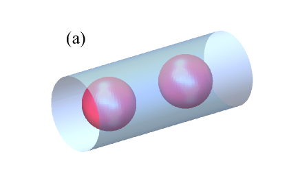
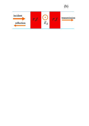
Figure 1: (a) Two particles inside a waveguide. (b) Model of two identical dielectric slabs in waveguide for the TE transmission. Coefficients $r$ and $t$ characterize reflection and transmission of each slab and $E_{z}$ corresponds to the direction of electric field inside the waveguide.

Manipulation of dielectric objects of a submicron size requires a strong optical confinement and high intensities than can be provided by diffraction-limited systems Yang . In order to overcome these limitations it was proposed to use subwave length liquid-core slot waveguides Almeida , fiber or photonic crystal (PhC) waveguides and cavities Barker ; Barth ; Hu . The technique simultaneously makes use of near-field optical forces to confine particles inside the waveguide and scattering/absorption forces to transport it. The ability of the slot or the PhC waveguides to condense the accessible electromagnetic energy to spatial scales as small as 60 nm also allows researchers to overcome the fundamental diffraction problem. However the consequence is that the cavity mode is strongly perturbed by the presence of a particle in its vicinity making standard PhC cavities unsuitable for noticeable back action effects. A clear evidence of the back action between a resonant field in a photonic crystal cavity and a single dielectric nanoparticle through the optical gradient forces was presented in Refs. Barth ; Juan ; Roichman ; Descharmes . As a result, the motion of the particles can considerably modify the light propagation.

The aim of the present paper is to study the time dependent back action effect for light propagation in a waveguide including a few dielectric microparticles with sizes comparable with the light wavelength, similar to an example shown in Fig. 1(a). An analogous problem was considered by Karásek et al. Karasek who numerically studied by the coupled dipole method a longitudinal optical binding between two microparticles in a Bessel beam.

There are several aspects tremendously complicating the consideration of spherical particles. (i) Spheres give rise to the problem of calculation of electromagnetic (EM) fields of both polarizations especially in the near-field zone. This problem can be solved only numerically by expanding of the waveguide propagating solutions over vector spherical functions and using the Lorenz-Mie theory Stratton ; Lock . (ii) For the scattering the Mie resonances could play important role for the dielectric spheres of high refractive index. (iii) All translational and rotational degrees of freedom are to be included in the dynamics of each particle.

In the present paper we model the particles with dielectric slabs inserted in a directional waveguide of a square cross-section $d\times d$ as shown in Fig. 1 (b). We take the perpendicular dimensions of the slabs very close to this cross-section. This allows us to consider only one-dimensional motion of particles and treat the problem analytically. This approach was applied for calculation of optical forces on dielectric particles in one-dimensional optical lattices Asboth ; Xuereb ; Sonnleitner by using the transfer matrix Markos . This model of a classical optomechanical system Aspelmeyer preserves all qualitative features of the initial problem as it can be described by the transfer matrix and predicts the important result of temporal oscillations of light transmittance caused by light-induced motion.

This paper is organized as follows. In Sec. II we remind the reader the formulas for the light pressure on a single particle in a waveguide. In Sec. III we formulate the model and consider motion of a single particle in the presence of a static “scattering center” inserted in the waveguide. In Sec. IV we investigate regimes of motion of two mobile particles. Section V presents the results for motion of a single particle inside a Fabry-Perot resonator. Conclusions and discussion of the results are given in Sec. VI.

II Forces on a dielectric slab in a waveguide

Motion of a particle in a vacuum- or air-filled waveguide is governed by the EM force $\mathbf{F}$ defined by the stress-tensor $T_{\alpha\beta}$ integrated over the surface elements $dS_{\beta}$ LL ; Pendry

$$F_{\alpha}=\int T_{\alpha\beta}dS_{\beta},$$ (1)

$$T_{\alpha\beta}=\frac{1}{4\pi}E_{\alpha}E_{\beta}^{*}-\frac{1}{8\pi}\delta_{\alpha\beta}|\mathbf{E}|^{2}+$$

$$\qquad\frac{1}{4\pi}H_{\alpha}H_{\beta}^{*}-\frac{1}{8\pi}\delta_{\alpha\beta}|\mathbf{H}|^{2},$$

where $\alpha$ and $\beta$ are the Cartesian indices. We concentrate on the basic propagating mode $\mbox{TE}_{10}$ having the following solution Jackson

$$H_{x} = H_{0}\psi(x)\cos\frac{\pi y}{d},$$

$$H_{y} = -\frac{ikd}{\pi}H_{0}\psi(x)\sin\frac{\pi y}{d},$$ (2)

$$E_{z} = \frac{i\omega d}{\pi}H_{0}\psi(x)\sin\frac{\pi y}{d},$$

where

$$\omega^{2}=\frac{\pi^{2}}{d^{2}}+k^{2},$$ (3)

$H_{0}$ is the field amplitude, $\psi(x)=e^{ikx}$ in the uniform waveguide, and the speed of light $c\equiv 1$.

To describe the EM field we need to know the scattering properties of each slab specified by the reflection and transmission coefficients $r,t$ which can be expressed with the transfer matrix $\mathbf{M}$ Markos

$$M_{11} = \cos(qa)+\displaystyle{\frac{i}{2}\left[\frac{q}{k}+\frac{k}{q}\right]\sin(qa)},$$

$$M_{12} = \displaystyle{\frac{i}{2}\left[\frac{q}{k}-\frac{k}{q}\right]\sin(qa)},~{}M_{22}=M_{11}^{*},~{}M_{21}=M_{12}^{*},$$

$$t = \displaystyle{\frac{1}{M_{22}}},~{}~{}r=\displaystyle{\frac{M_{12}}{M_{22}}},$$ (4)

where $a$ is the slab thickness. Here $q$ is wave vector component along the $x$-axis given by:

$$q^{2}=\epsilon k^{2}+(\epsilon-1)\frac{\pi^{2}}{d^{2}},$$ (5)

where $\epsilon$ is the dielectric constant of the slabs shown in Fig. 2.

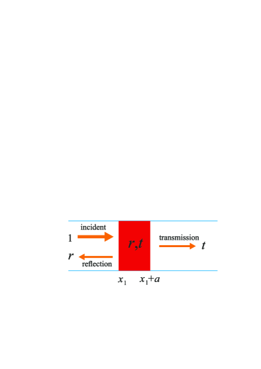
Figure 2: Transmission and reflection through a single slab.

Let us consider force acting on such a slab. Its presence in the waveguide modifies the components of the electromagnetic field in the $\mbox{TE}_{10}$ mode (II) as:

$$\frac{H_{x}}{H_{0}}=\cos\frac{\pi y}{d}\left\{\begin{array}[]{l}e^{ik(x-x_{1})}+re^{-ik(x-x_{1})},\quad x<x_{1},\cr\cr te^{ik(x-x_{1}-a)},\quad x>x_{1}+a,\cr\end{array}\right.$$ (6)

$$\frac{H_{y}}{H_{0}}=-\frac{ikd}{\pi}\sin\frac{\pi y}{d}\left\{\begin{array}[]{l}e^{ik(x-x_{1})}-re^{-ik(x-x_{1})},\quad x<x_{1},\cr\cr te^{ik(x-x_{1}-a)},\quad x>x_{1}+a,\cr\end{array}\right.$$ (7)

$$\frac{E_{z}}{H_{0}}=\frac{i\omega d}{\pi}\sin\frac{\pi y}{d}\left\{\begin{array}[]{l}e^{ik(x-x_{1})}+re^{-ik(x-x_{1})},\quad x<x_{1},\cr\cr te^{ik(x-x_{1}-a)},\quad x>x_{1}+a.\cr\end{array}\right.$$ (8)

Substituting these solutions into Eq. (1) we obtain the light pressure

$$P=P_{0}(1+|r|^{2}-|t|^{2})=2P_{0}|r|^{2},$$ (9)

where

$$P_{0}=\frac{H_{0}^{2}}{8\pi}\left(\frac{kd}{\pi}\right)^{2}.$$ (10)

III Dynamics of a single particle in the presence of a scattering center

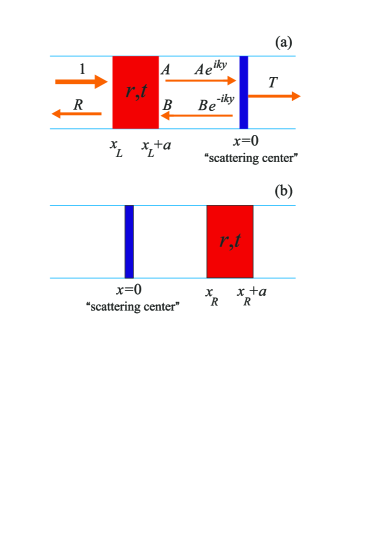
Figure 3: Immobile scattering center-related geometries. (a) Movable slab is on the left from the scattering center and $y=-(x_{L}+a)$. In this geometry we consider two types of the static elements: one optically equivalent to the movable slab and an ideal mirror. $A$ and $B$ are the field amplitudes. (b) Movable slab is on the right from the scattering center, which here is optically equivalent to the slab.

The situation described in the previous section changes dramatically if another element, besides the mobile dielectric particle is inserted in the waveguide. In particular, we insert at $x=0$ an immobile particle (“scattering center”) characterized by light transmission and reflection coefficients, as shown in Fig. 3. Then the solution for the EM field and therefore, the force acting on the mobile particle become dependent on its distance to the center and cause various regimes of the slab motion. Here we concentrate on this motion driven by the optical force $F_{j}(x_{j})$ and the corresponding potential $U_{j}(x_{j})$ described by equation

$$m\ddot{x}_{j}+6\pi\eta d\dot{x}_{j}=F_{j}(x_{j})=-\displaystyle{\frac{dU_{j}}{dx_{j}}},$$ (11)

resulting, as we will show, in the time oscillations of the light transmittance through the waveguide. Index $j=L,R$ enumerates the particle positioned on the left or on the right from the immobile center, $m=\rho ad^{2}$ is the particle mass ($\rho$ is the material density), and $6\pi\eta d$ is the linear drag coefficient for a particle in a medium of viscosity $\eta$ Praveen ; coefficient . In what follows we choose the dielectric constant of the slab $\epsilon=4$ (glass), its width $a=d/2$, and zero initial velocity. We neglect imaginary part of the dielectric constant and corresponding contribution into the optical force due to its smallness in the visible light frequency domain Kitamura .

We begin with the realization shown in Fig. 3(a). Similar to Ref. Xuereb , we write the equation for the ingoing and outgoing amplitudes of waves $\psi(x)$ describing the EM field components in each region of the waveguide (Fig. 3):

$$\left[\begin{array}[]{c}A\\ B\end{array}\right]=\mathbf{M}\left[\begin{array}[]{c}1\\ R\end{array}\right],\quad\left[\begin{array}[]{c}T\\ 0\end{array}\right]=\mathbf{M}\left[\begin{array}[]{c}Ae^{iky}\\ Be^{-iky}\end{array}\right],$$ (12)

where we assumed optical equivalence of the scattering center and the movable slab, $y=-(x_{L}+a)$ is the distance between the particles, and the matrix $\mathbf{M}$ is given by Eq. (II). The total transmission and reflection amplitudes can be expressed as Markos ; BW

$$R=r+\displaystyle{\frac{t^{2}re^{2iky}}{1-r^{2}e^{2iky}}},\qquad T=\frac{t^{2}e^{iky}}{1-r^{2}e^{2iky}}.$$ (13)

Substituting the solution of Eq. (12) into Eq. (1) we find the forces acting on the slab ($F_{L}$) and the scattering center ($F_{\rm SC}$) as

$$F_{L}(y)=P_{0}d^{2}\left[1+|R|^{2}-|A|^{2}-|B|^{2}\right],$$

$$F_{\rm SC}(y)=P_{0}d^{2}\left[|A|^{2}+|B|^{2}-|T|^{2}\right]$$

$$=-F_{L}(y)+2P_{0}d^{2}|R|^{2},$$ (14)

respectively. The forces depend only on the distance $y$.

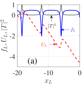
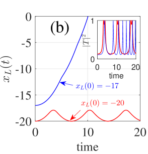
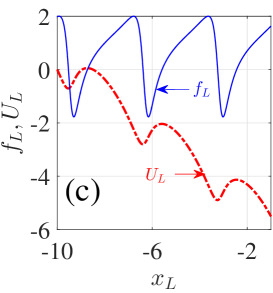
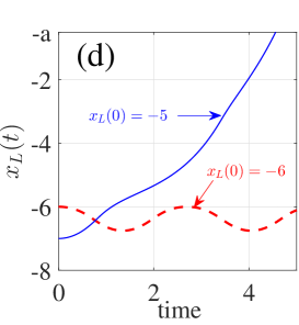
Figure 4: (a) The optical force (III) (solid line), the corresponding potential (dot line), and the light transmission (dash-dot line) for the first (left) moving particle and the immobile (right) particle positioned at $x_{R}=0$. (b) The corresponding time evolution of the left particle position and light transmission for two choices of initial positions. Figures (c) and (d) correspond to an immobile mirror with at the position $x_{R}=0$. The parameters of the slab are $a=d/2,\epsilon=4,k=1/2$. The evolution in (a)-(d) is considered frictionless with $\gamma=0$. The coordinates, forces, and time are given in the units of $d$, $P_{0}d^{2},$ and $\Omega_{0}^{-1},$ respectively (see Eq. 15).

The magnitude of the force acting on the particle of the cross-section $d^{2}$ can be evaluated with Eq. (1) as $P_{0}d^{2},$ that is proportional to the injected into the waveguide light power $W_{0}$ Nemoto ; Romero . At $W_{0}=100$ mW, this yields the typical optical force $F$ of the order of 1 nN. The characteristic frequency of the oscillations, which we need for dimensionless equations of motion, can be estimated by an order of magnitude in the physical units as $\Omega_{0}=\sqrt{F/dm}$. Since the dielectric particles of our interest with the size of the order of $10^{-4}$ cm have masses $m$ of the order of 1 pg, these oscillations show characteristic frequencies of the order of $2\pi\times 100$ kHz Romero , much lower than the light frequency. Below we show as dependent on the initial conditions motion of particles can be bounded with characteristic frequency substantially less than $\Omega_{0}$ or unbounded on times considerably larger than $\Omega_{0}^{-1}$. The corresponding velocity of $\Omega_{0}d$ being of the order of 10 cm/s allows one to consider the light transmission adiabatically. On the other hand, the thermal velocity of a particle of the mass of 1 pg at the room temperature is of the order of 1 mm/s, which allows one to a good approximation neglect the random Brownian motion.

Introducing the dimensionless coordinate via $d,$ force as $P_{0}d^{2}$ and mass $m\equiv 1$ (leading to the time unit as $\Omega_{0}^{-1}$), we can write Eq. (11) in dimensionless form

$$\ddot{x}_{j}+\gamma\dot{x}_{j}=f_{j}(x_{j}),$$ (15)

where $f_{j}$ is the dimensionless force acting on the $j$-th particle Praveen , and $\gamma$ is expressed in the physical units as

$$\gamma=6\pi\eta\sqrt{\frac{d}{P_{0}m}}.$$ (16)

For water with $\eta_{w}\approx 10^{-2}$ $\mbox{dyn}\cdot\mbox{s/cm}^{2}$, Eq. (16) yields the dimensionless $\gamma$ of the order of 10 for the injected light power $W_{0}$ of the order of 100 mW. For the air with $\eta_{a}\approx 0.01\eta_{w}$, the value of $\gamma$ at the same $W_{0}$ is of the order of 0.1, corresponding to a relatively weak damping. With the increase in the light power, the effect of viscous friction decreases as $W_{0}^{-1/2}.$

For the realization corresponding to Fig. 3(a), we show in Fig. 4(a) the light transmittance through two particles, optical force $f_{L}(x_{L})$ and the corresponding potential

$$U_{L}(x_{L})=-\int_{x_{L}(0)}^{x_{L}}f_{L}(x)dx,$$ (17)

where $x_{L}(0)$ is the initial position of the particle. One can see that in the Newtonian regime $\gamma=0$ describing exactly particles in the vacuum or approximately in the air, we have either the bounded or unbounded time evolution of the positions, dependent on $x_{L}(0)$ as presented in Figs. 4 (a) and 4 (b). The characteristic period of the potential is determined by the wave vector $k$. Two particles in the waveguide form a Fabry-Perot resonator (FPR) structure in which the transmittance $|T|^{2}$ shows sharp peaks when distance between the slab and the scattering center equals integer number of half wave lengths. Then the wave function amplitude $\psi(x)$ inside the resonator is maximal to give rise to resonant behavior of the optical force acting on the walls of the resonator. Indeed, one can see that the force follows the light transmittance with sharp resonant negative dips. As the result the potential $U_{L}(x_{L})$ in (17) acquires a tilted periodic shape with the particle dynamics qualitatively different from that in a simple periodic one.

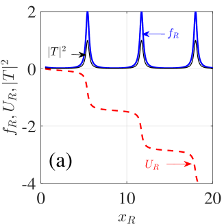
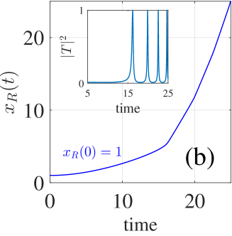
Figure 5: (a) The optical force (III) (solid line), the corresponding potential (dot line), and the light transmission (dash-dot line) for the immobile left particle positioned at $x_{L}=0$. (b) The corresponding time evolution of the position of the right particle and light transmission (in the inset) for $\gamma=0.$ The parameters of “scattering center” and the slab are identical with $a=d/2,\epsilon=4$, and $k=1/2$. The coordinates, forces, and time are given in the units of $d$, $P_{0}d^{2},$ and $\Omega_{0}^{-1},$ respectively (see Eq. 15).

Respectively, as depends on the initial position of the particle, the time evolution shows oscillations or a motion until the particle touches the immobile element at $x_{L}=-a$ as shown in Fig. 4(b). After this event the evolution needs a special analysis which goes beyond the scope of the present paper. The inset in Fig. 4(b) shows that the choice of the initial position strongly changes the evolution of the light transmission through the particles with the left particle dragged by light. Here we obtain oscillations with growing frequency since the distance between particles increases with time with acceleration caused by nonzero mean optical force. For the periodic oscillations of the left particle shown by the red line in Fig. 4(b) the time oscillations of light transmission are periodic with a few harmonics. The appearance of this multi-frequency behavior is a result of anharmonicity of the binding potential $U_{L}$ shown in Fig. 4(a).

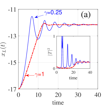
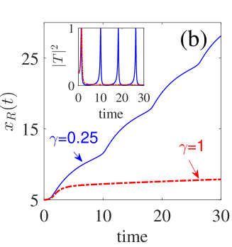
Figure 6: Time evolution of the left (a) or right (b) particle coordinate and light transmission in a viscous medium with $x_{L}(0)=-17$ and $x_{R}(0)=5$. The values of $\gamma$ are shown near the plots. The coordinates, forces, and time are given in the units of $d$, $P_{0}d^{2},$ and $\Omega_{0}^{-1},$ respectively (see Eq. 15).

Figure 5 shows the case corresponding to Fig. 3(b). Again the optical force follows the resonant dependence of the transmittance as a function of the distance between the particles with however positive peaks. Unlike the case of Fig. 3(a), the motion of the particle here is always unbounded. Respectively, we have time oscillations of transmittance in Fig. 5 (b) with growing frequency. Effects of damping on the motion of the particles with the corresponding time evolution of light transmittance are shown in Fig. 6.

IV Evolution in system of two mobile particles

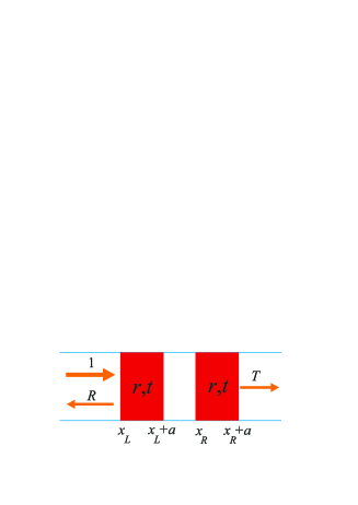
Figure 7: Two mobile slabs geometry.

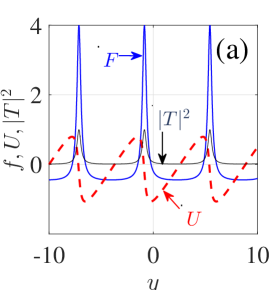
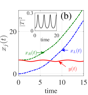
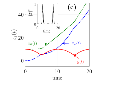
Figure 8: (a) Force and potential vs function of distance between two mobile particles. Time evolution of coordinates and distance between the particles for the initial positions $x_{L}(0)=0$ and $x_{R}(0)=6.5$ (b) and $x_{R}(0)=10$ (c). The coordinates, forces, and time are given in the units of $d$, $P_{0}d^{2},$ and $\Omega_{0}^{-1},$ respectively (see Eq. (15)).

For identical particles shown in Fig. 7 we obtain similarly to Eqs. (11) and (III) the following dimensionless equation of motion:

$$\ddot{y}+\gamma\dot{y}=\widetilde{f}(y)=-\displaystyle{\frac{d\widetilde{U}}{dy}},$$ (18)

where $\widetilde{f}(y)=f_{R}(y)-f_{L}(y)$. The “force” $\widetilde{f}(y)$ depends only on the distance between particles $y=x_{R}-x_{L}$ and is shown in Fig. 8(a). Surprisingly, the corresponding “potential” $\widetilde{U}(y)$ shows only periodic dependence on the distance $y,$ different from the interaction considered in the previous Section and similar to the optical binding of atomic clouds Asboth due to the standing EM waves. The characteristic “potential” height $\widetilde{U}_{0}$ can be estimated as $Fd\sim 10^{-8}\mbox{ erg}$. Since we consider the light incident from the left, the inversion symmetry is broken resulting in $\widetilde{U}(y)\neq\widetilde{U}(-y)$.

Figure 8 demonstrates that the time dependence of the light transmittance strongly depends on the initial distance between the particles. For the distance $y(0)$ when the potential is close to the minimum, the positions evolve in time approximately preserving the interparticle distance. Respectively, the light transmittance oscillates with time approximately harmonically as shown in the inset of Fig. 8(b). However if the initial position is far from the minimum, the nonparabolicity of the potential becomes important and the time dependence of the transmittance acquires higher harmonics. Interactions presented in Fig. 8 show more variety than the optical binding of small dielectric particles in the Bessel beams Karasek and in the random fields Brugger .

V Dynamics of a particle inside a Fabry-Perot resonator

The analysis of the system of dielectric slabs in the waveguide allows us to consider analytically optical driving of a dielectric particle by EM fields in resonant cavities. The cavity can be modeled by two immobile dielectric slabs and the particle is modeled by a mobile slab as shown in Fig. 9.

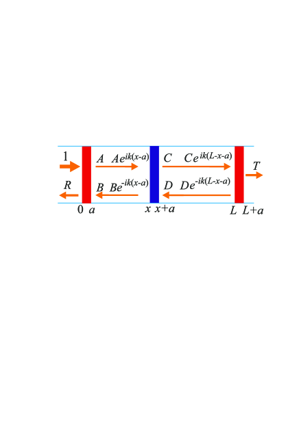
Figure 9: Two slabs with dielectric constant $\epsilon_{m}$ shown by red color fixed at $x=0$ and $x=L$ form FPR (cavity). The third slab with the dielectric constant $\epsilon$ can move inside the resonator.

The solutions of the EM field equations are given by the transfer matrices

$$\left[\begin{array}[]{c}A\\ B\end{array}\right]=\mathbf{m}\left[\begin{array}[]{c}1\\ R\end{array}\right],\quad\left[\begin{array}[]{c}T\\ 0\end{array}\right]=\mathbf{m}\left[\begin{array}[]{c}Ce^{ik(L-x-a)}\\ De^{-ik(L-x-a)}\end{array}\right]$$ (19)

for the walls of the resonator and

$$\left[\begin{array}[]{c}C\\ D\end{array}\right]=\mathbf{M}\left[\begin{array}[]{c}Ae^{ik(x-a)}\\ Be^{-ik(x-a)}\end{array}\right]$$ (20)

for the embedded movable slab. Here the matrix $\mathbf{M}$ is given by Eq. (II), $\mathbf{m}$ has the elements

$$m_{11} = \cos(q_{0}a)+\displaystyle{\frac{i}{2}\left[\frac{q_{m}}{k}+\frac{k}{q_{m}}\right]\sin(q_{m}a)},$$ (21)

$$m_{12} = \displaystyle{\frac{i}{2}\left[\frac{q_{m}}{k}-\frac{k}{q_{m}}\right]\sin(q_{m}a)},~{}m_{22}=m_{11}^{*},~{}m_{21}=m_{12}^{*},$$

and

$$q_{m}^{2}=\epsilon_{m}k^{2}+(\epsilon_{m}-1)\frac{\pi^{2}}{d^{2}}.$$ (22)

Similar to Eq. (9) we have for the optical pressure on the mobile particle Asboth

$$P(x)=P_{0}\left[|A(x)|^{2}+|B(x)|^{2}-|C(x)|^{2}-|D(x)|^{2}\right].$$ (23)

The corresponding potential $U(x)$ is presented in Fig. 10. One can see that it strongly depends on the dielectric constant of the walls of the resonator, i.e. on its openness. For $\epsilon_{m}$ close to $\epsilon$ the potential holds local minima capable to bind the particle at the corresponding positions. This result is reminiscence of electron transmission through the well potential relief with two different potential wells Ricco .

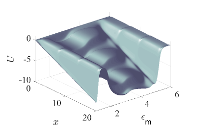
Figure 10: The potential $U(x)$ (in the units of $P_{0}d^{3}$) vs the particle position (in the units of $d$) and the dielectric constant of the FPR walls for $\epsilon=4,a=1/2,k=1/2$, and $L=20$.

Time evolution of the particle position in the FPR is shown in Fig. 11(a) for two initial $x(0).$ The first position, $x(0)=6.5,$ yields oscillations in the vicinity of a local potential minimum shown in Fig. 10. An extremely nonlinear profile of the potential over the particle position gives rise to the shape of the corresponding time oscillations of the light transmittance shown in Fig. 11(b) by dashed red line. The second choice, $x(0)=4.5,$ corresponds to the accelerated time evolution until the particle will reach the right wall. This motion corresponds to the time behavior of the transmittance as shown in Fig. 11(b) by blue solid line.

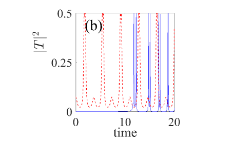
Figure 11: Time evolution of the particle position (a) and transmittance (b) for the same parameters given in Fig. 10, $\epsilon_{m}=3$ and $L=20$. The initial position of the particle is $x(0)=6.5$ (red dash-dot lines) and $x(0)=4.5$ (blue solid lines). The coordinates are given in the units of $d.$

VI Summary and conclusions

Although the replacement of the particles by slabs as shown in Fig. 1 is a significant simplification, it preserves the main qualitative features of the light transmittance in a waveguide with embedded particles as described in general terms by a transfer-matrix dependent on the positions and optical properties of these particles. When one particle is inserted in a waveguide, it is subject to a radiation pressure of the propagating light. This pressure does not depend on the position of the particle and produces its constant acceleration in the vacuum or drags it in a viscous medium with a constant velocity. The transmittance of light through the particle remains position and time-independent. The situation changes dramatically if at least two particles are inserted in the waveguide. Because of different light pressure acting on the particles the interparticle distance changes with time. Respectively, the transmittance given by the Fabry-Perot resonator transfer matrix equations (13) acquires a time dependence.

To describe the light-induced interaction between the particles one can introduce an effective system-dependent potential. This potential usually has a tilted (or a simple, as depends on the system realization) periodic shape, where the evolution of the interparticle distance can be bounded or unbounded. As a result, the light transmittance shows a rich variety of time-dependent behaviors in the form of time oscillations either with a few harmonics for a bounded motion or with a growing frequency for the unbounded one. The characteristic period of the oscillations in the light transmittance shown in the paper is of the order of $10^{-5}$ s for the propagating light power of the order of 100 mW. Therefore, by changing the laser light power and direction one can achieve different regimes of the particles motion. Similar modifications can be achieved by choosing different materials for the movable particles and static elements such as the “scattering center” in Fig. 3 or walls of the Fabry-Perot resonator in Fig. 9.

It is important to mention that recent publications confirm the presence of this phenomenon in different experimental set-ups: two rotating dielectric microparticles Arita and density oscillations of swimming bacteria confined in microchambers Paoluzzi . Both systems show the characteristic frequencies of light modulation in the sound range. Thus, the analysis of the time dependence of the light transmittance paves a way for manipulating and monitoring motion of the particles in optical waveguides.

- (1) A. Ashkin, J.M. Dziedzic, J.E. Bjorkholm, and S. Chu, Opt.Lett. 11, 288 (1986).
- (2) M.M. Burns, J.-M. Fournier, and J.A. Golovchenko, Phys. Rev. Lett. 63, 1233 (1989).
- (3) Y. Ogura, N. Shirai, and J. Tanida, Appl. Optics 41, 5645 (2002).
- (4) A.H.J. Yang, S.D. Moore, B.S. Schmidt, M. Klug, M. Lipson, and D. Erickson, Nature 457, 71 (2009).
- (5) O. Brzobohatý, V.Karásek, M.S. Šiler, L. Chvátal, T. Čižmár, and P. Zemánek, Nat. Photonics, 7, 123 (2013).
- (6) D.G. Grier, Nature 424, 810 (2003).
- (7) T.J. Kippenberg and K.J. Vahala, Science 321, 1172 (2008).
- (8) P.F. Barker and M.N. Shneider, Phys. Rev. A 81, 023826 (2010).
- (9) V.R. Almeida, Q. Xu, C.A. Barrios, and M. Lipson, Opt. Lett. 29, 1209 (2004).
- (10) M. Barth and O. Benson, Appl. Phys. Lett. 89, 253114 (2006).
- (11) J. Hu, S. Lin, L.C. Kimerling, and K. Crozier, Phys. Rev. A 82, 053819 (2010).
- (12) M.L. Juan, R. Gordon, Y. Pang, F. Eftekhari, and R. Quidant, Nature Phys. 5, 915 (2009).
- (13) Y. Roichman, B. Sun, A. Stolarski, and D.G. Grier, Phys. Rev. Lett. 101, 128301 (2008).
- (14) N. Descharmes, U.P. Dharanipathy, Zh. Diao, M. Tonin, and R. Houdre, Phys. Rev. Lett. 110, 123601 (2013).
- (15) V. Karásek, T. Čiz̆már, O. Brzobohatý, P. Zemánek, V. Garcés-Chávez, and K. Dholakia, Phys. Rev. Lett. 101, 143601 (2008).
- (16) J. A. Stratton Electromagnetic Theory (McGraw-Hill, New York, 1941).
- (17) J.A. Lock, Appl. Optics, 43, 2532 (2004).
- (18) J. K. Asbóth, H. Ritsch, and P. Domokos, Phys. Rev. A77, 063424 (2008).
- (19) A. Xuereb, P. Domokos, J. Asbóth, P. Horak, and T. Freegarde, Phys. Rev. A 79, 053810 (2009).
- (20) M. Sonnleitner, M. Ritsch-Marte, and H. Ritsch, EPL 94, 34005 (2011).
- (21) P. Markos and C.M. Soukoulis, Wave Propagation, From Electrons to Photonic Crystals and Left-Handed Materials (Princeton University Press 2008), Ch. 10.
- (22) M. Aspelmeyer, T. J. Kippenberg, and F. Marquardt, Rev. Mod. Phys. 86, 1391 (2014).
- (23) L.D. Landau and E.M. Lifshitz, Electrodynamics of Continuous Media (Pergamon Press, New York, 1960), Secs. 15, 34, and 56.
- (24) M.I. Antonoyiannakis and J.B. Pendry, Phys. Rev. B 60, 2363 (1999).
- (25) J.D. Jackson, Classical Electrodynamics (Johm Willey and Sons, Inc. New York, 1962), Ch. 8.
- (26) P. Praveen, Yogesha, S.S. Iyengar, S. Bhattacharya, and S. Ananthamurthy, Appl. Opt. 55, 585 (2016).
- (27) The numerical coefficient in the viscosity force expression depends on the shape of the partice with being, technically speaking, correct only for a perfect sphere. Nevertheless, we will use it as an order-of-magnitude estimate.
- (28) R. Kitamura, L. Pilon, and M. Jonasz, Appl. Optics 46, 8181 (2007).
- (29) M. Born and E. Wolf, Principles of Optics: Electromagnetic Theory of Propagation, Interference and Diffraction of Light, Cambridge University Press, (1999).
- (30) S. Nemoto and H. Togo, Appl. Optics 37, 6386 (1998).
- (31) O. Romero-Isart, A.C. Pflanzer, M.L. Juan, R. Quidant, N. Kiesel, M. Aspelmeyer, and J.I. Cirac, Phys. Rev. A 83, 013803 (2011).
- (32) G. Brügger, L.S. Froufe-Pérez, F. Scheffold, and J.J. Sáenz, Nat. Commun. 6, 7460 (2015).
- (33) B. Ricco and M. Ya. Azbel, Phys. Rev. B 29, 1970 (1984).
- (34) Y. Arita, M. Mazilu, T. Vettenburg, E.M. Wright, and K. Dholakia, Opt. Lett. 40, 4751 (2015).
- (35) M. Paoluzzi, R.Di Leonardo, and L. Angelani, Phys. Rev. Lett. 115, 188303 (2015).